Graceful Degradation and Related Fields

Abstract

When machine learning models encounter data which is out of the distribution on which they were trained they have a tendency to behave poorly, most prominently over-confidence in erroneous predictions. Such behaviours will have disastrous effects on real-world machine learning systems. In this field graceful degradation refers to the optimisation of model performance as it encounters this out-of-distribution data. This work presents a definition and discussion of graceful degradation and where it can be applied in deployed visual systems. Following this a survey of relevant areas is undertaken, novelly splitting the graceful degradation problem into active and passive approaches. In passive approaches, graceful degradation is handled and achieved by the model in a self-contained manner, in active approaches the model is updated upon encountering epistemic uncertainties. This work communicates the importance of the problem and aims to prompt the development of machine learning strategies that are aware of graceful degradation.

1 Introduction

Over the last decade the amount of data that is available in our society has increased massively, from football match statistics to personal information, data has become another currency with which companies compete with one another. With this data often being unstructured, the necessity for analysts and data scientists has increased across every industry in the world. As such, the tools and algorithms that they use have seen significant surges in development, both in the academic and commercial environment. The field of machine learning has been progressing at an unprecedented rate, this progress being led by research staff at universities across the world. Heavy investment from tech giants such as Google and Microsoft and newcomers such as DeepMind and OpenAI has prompted collaboration with universities, allowing greater acceleration in progress. Hardware manufacturers such as ARM and Nvidia have shifted towards giving AI a central role in their business models, hence, both ends of the technology industry are contributing resources to the field that help facilitate this surge in progress.

The data passed to these systems has increased in volume and complexity, making the manual extraction of features unfeasible. Consequently, the less complicated algorithms that once dominated the field have seen less development. In their place deep neural networks have seen a significant rise and have sparked what is often referred to as a ‘Golden Age’ of machine learning. Deep learning is effective because of its unparalleled ability to find meaningful features and representations in data and its ability to generalise these across large amounts of data.

This has prompted much interest from many industries around the world, from the defence to the pharmaceutical sector, companies are forming the same academic alliances as tech companies to help improve the products and services they can offer. Indeed this has sparked many developments that will be influential for years to come, for example DeepMind’s AlphaFold2 (Jumper (2020)), a deep learning system that has solved the 50-year-old protein folding problem in biochemistry first presented by Levinthal (1969).

But these systems are not without flaws. For example DeepMind’s other groundbreaking system, AlphaGo, predicted with high certainty that it would win the one match it lost against the world champion Go player. That is until a pivotal move changed the game (Silver et al. (2017)).

This is not something limited to these state-of-the-art systems, but is a problem of many deep learning systems. In vision systems, which will serve as the focus of this survey, these effects might occur when encountering data outside of the training distribution. These will cause uncalibrated models to output over-confident, yet erroneous predictions (Li & Hoiem (2020)). When deployed in safety-critical environments such mistakes will have catastrophic consequences, thus in many environments it is critical that the machine learning systems be implemented in a safe and responsible manner. To utilise deep learning in sectors that have real-world consequences it is important to ensure these shortcomings are managed responsibly. To that end, such techniques should be integrated into systems with the concept of graceful degradation built into them.

1.1 Defining Graceful Degradation

Outside of the machine learning environment graceful degradation refers to the notion of making a system resilient to disruption in its architecture (Herlihy & Wing (1991)). That is, when parts of the system are inoperable, the system’s performance will degrade in the most efficient way possible.

In machine learning, achieving graceful degradation can be interpreted as optimising the drop in performance of a model as it processes data that is further from the distribution on which it was trained. These are commonly known as out-of-distribution errors(Hendrycks & Gimpel (2016)). Graceful degradation is the notion of minimising their effect.

The problem with out-of-distribution errors when applying machine learning is not the errors themselves, it is the manner in which such errors occur. State-of-the-art machine learning techniques can achieve beyond human accuracy on some tasks as demonstrated by the the pursuit of high accuracies in the ImageNet challenge, currently being led by Dosovitskiy et al. (2020). However, when such models are presented images outside of their training distributions, they are often susceptible to making over-confident erroneous predictions (Li & Hoiem (2020)).

There are a variety of ways one can correct for such effects. Fundamentally, the model should understand the class distribution on which it is trained and know when it encounters something outside of it. That is, the model should understand when it is uncertain.

Then the way in which the model deals with uncertainty defines the approaches that can be taken in achieving graceful degradation. For example, the operator may wish for the model to appropriately signify when it is low on confidence and do this consistently when encountering out-of-distribution data. Alternatively, the operator may instead wish for the model to function on out-of-distribution data and have it trained to recognise objects without having prior examples of them, a method known as zero-shot learning. There could also be a compromise between these approaches whereby the model does not offer a fine-grained classification, but instead offers a coarser-level classification, recognising the hierarchical nature of its inputs. Alternatively, it may be more desirable for the model retrain on the unseen distribution. This might be in an individual data point manner by identifying areas in the distribution that lack the desired sample density, it might be shifting to an entirely new domain of data, or it may be training on an entirely different problem.

To give some of these methodologies context, a number of vignettes are detailed below that can help provide some clarity.

Disaster Response Drone

A disaster response drone might be trained to recognise various scenes in natural disaster scenarios as a way of quickly surveying an area involved in such a disaster. For example, the surrounding coastline in the aftermath of a tsunami may need to be surveyed for notable features such as flooded areas, collapsed buildings, and also unaffected areas to inform sensible allocation of resources. The visual system behind such a drone could be trained in a number of ways. It could be desirable to inform the operator when it is processing images outside of its expertise. Here, the model could express its uncertainty in such scenarios and recommend manual cataloguing of the area. Alternatively, it may be given explicit examples of types of vehicles, but only semantic information of other types and is expected to classify these should it come across them, highlighting the classification as zero-shot. Finally, it might instead be required to give a partial classification, such as the category of an object e.g., it might recognise an area of land is flooded, but may not be able to infer the type of land that is underneath. (Some examples of vision models in drone systems are given in: Zientara et al. (2018), van Gemert et al. (2015) ,Radovic et al. (2017))

Smart Cities

Cities process large amounts of data every day and as smart city systems become more prevalent, manually processing the data will become intractable. Hence, it may be beneficial to automatically process some of the data seen by the system. The system may encounter information that is not within its training distribution, that it could not process confidently. This could be handled in a variety of ways. The information could be communicated to and processed by an operator, which would allow the model to update its parameters in this area of the distribution. The model could also be having difficulty due to seasonal changes in the information, such as increased traffic flow around public holidays and can be retrained on examples of this. Finally, the model could be retrained to recognise situations with different volumes of pedestrians and the changes that come with them, such as areas which have an increased chance hooliganism at times surrounding football matches. Ideally, a single system would be able to identify all of the aforementioned scenarios, but this is not always practical due to computational constraints in a lightweight system. Hence, there may be a need to retrain the model in an intelligent manner. (Some examples of artificial intelligence models in a similar domain are given in: Ai & Kwon (2020), Kihara et al. (2019))

The applications of graceful degradation can be split into two sections, one where the system deals with out-of-distribution data in a self-contained manner, and one where the system can take additional inputs to improve its performance in the observed distribution. These two approaches can be split into passive and active approaches.

1.2 Passive vs Active

When dealing with out-of-distribution data a gracefully degrading system should be able to operate in a desirable manner. Broadly speaking, this can come in one of two ways: One whereby the model identifies it as out-of-distribution and gives an accordingly conditioned output, then another whereby the model requires additional information in order to continue operating effectively. These are passive approaches and active approaches, respectively.

In passive approaches to graceful degradation, the model is a self-contained system that can provide a solution to the graceful degradation problem without requiring further input. An example of a passive approach might include simply providing good uncertainty estimates in the drone vignette, whereby the system informs the operator when it is uncertain about what it is seeing. Such approaches will be considered in section 2.1. Another example might be where the model can attempt to classify out-of-distribution data without ever being shown examples of it, such zero-shot classification is discussed in section 2.2. Finally, there might be a middle ground between these two, whereby the model cannot classify an item, but it can go some way to indicate what it is viewing, taking into account the class hierarchy and giving a coarser-grained prediction. This is discussed in section 2.3.

In contrast, rather than remain static, active approaches seek to improve their understanding of the task and its data once encountering uncertainties. This will be done by updating or retraining the model. The degree to which this update changes can separate the active approaches. The model might lack understanding in a particular area of the data distribution and require annotation from an operator to inform a parameter update. In section 3.1 these small changes will be discussed, in relation to active and continual learning paradigms in the field. The model might be encountering too much out-of-distribution data for small updates to help, hence it may need to be completely retrained for a new distribution/domain. This problem will be discussed in the context of domain adaptation in section 3.2. Finally, the system may now be encountering completely new data thus changing its task. Here, models would be required to quickly learn new tasks and this could be solved by meta-learning. These approaches will be discussed in section 3.3.

A core idea in all of these scenarios is the model understanding when it is uncertain and out of its depth. Hence, it will be important to understand the various ways of defining uncertainty. This will be covered briefly in the next section.

1.3 Understanding Uncertainty

In order to investigate uncertainties in classification, it is important to first understand the various interpretations of uncertainty in the machine learning field and how they can be quantified, starting with the latter.

To understand a model’s uncertainty, it needs to be quantified. There are variety of ways to do this and in the deep learning field usually the output of the model is used as a means of obtaining the uncertainty. This output is most commonly in the form of a softmax distribution representing a probability over the class space, a technique popularised by Duan et al. (2003). This is presented mathematically in equation 1, where $p(y_{i})$ is the probability of class $i$ and $N$ is the number of classes. Here, $y$ refers to the output of a neural network’s last layer, representing prediction values for each , $i$, class in a classification task. The softmax function converts these raw numbers into probabilities.

This probability distribution is often passed into the cross entropy formula, which was first presented by Good (1952). This is shown in equation 2, where, $q$ is the estimation from the machine learning algorithm, often using a soft-max, and $p$ is the statistical probability accounting for the distribution of classes in the data. These are often used as confidence scores, something that can be interpreted as the inverse of uncertainty.

$$p(y_{i})=\frac{e^{y_{i}}}{\sum\limits_{j=1}^{N}e^{y_{j}}}$$ (1)

$$I(p,q)=-\sum_{i=1}^{N}p(y_{i})\log q(y_{i})$$ (2)

There also exist a variety of evaluation measures in the field that are related to confidence and will use confidence scores in their calculation. For example, the E99 error is the error rate in classifications where the classifier records 99% certainty in its prediction. This is a quantity discussed in a recent paper by Li & Hoiem (2020), which analyses over-confidence in erroneous classifications on out-of-distribution data. Expected calibration error (ECE), which was first described as such by Naeini et al. (2015), measures whether or not the classifier “knows what it knows”, as it is designed to measure the alignment between the accuracy and the confidence by summating the difference between them over given intervals. There also exists the Brier score, first developed for weather prediction by Brier (1950). In this score the difference is taken between the confidence in the correct the label and the number 1. Hence, this is optimised when the confidence in the correct label is maximised. Such measurements are useful in the field of graceful degradation, as they emphasise where confidence is misplaced. Hence, a variety of confidence calculation methods are compatible with gracefully degrading systems.

Uncertainty does not only exist within the trained distribution. In the graceful degradation problem it is the uncertainty on data outside of the trained distribution that is more important. These types of uncertainty are known as aleatoric and epistemic uncertainty (Hüllermeier & Waegeman (2020)). In machine learning, aleatoric uncertainty is the uncertainty arising due to the natural stochasticity in the data, it can be likened to the ability for the model to interpolate effectively. On the other hand, epistemic uncertainty arises due the training data insufficiently representing the data being observed by the model. That is, the model is encountering data it is not familiar with. This might be due to insufficient training data in the area, or it might be due to the data being entirely out-of-distribution, and the model has failed to extrapolate effectively. Hence, epistemic uncertainty is the most relevant error in the graceful degradation problem as it concerns error due to out-of-distribution samples.

A useful graphical tool in understanding uncertainty can be seen in figure 1. This figure is known as a simplex and each vertex represents a class in the dataset. This makes a simplex a $K-1$ dimensional object, where $K$ is the number of classes. The particular example shown in figure 1 has been taken from a paper by Malinin & Gales (2018). Here there are 3 classes and a lighter colour in this space equates to a higher probability of placing the sample there. Thus, for a confident prediction a vertex will be highlighted like in figure 1(a), then for uncertain predictions there is figure 1(b) for an aleatoric case, and figure 1(c) for the epistemic case. Figure 1 represents the optimal response of a classifier to out-of-distribution errors, as total uncertainty is returned.

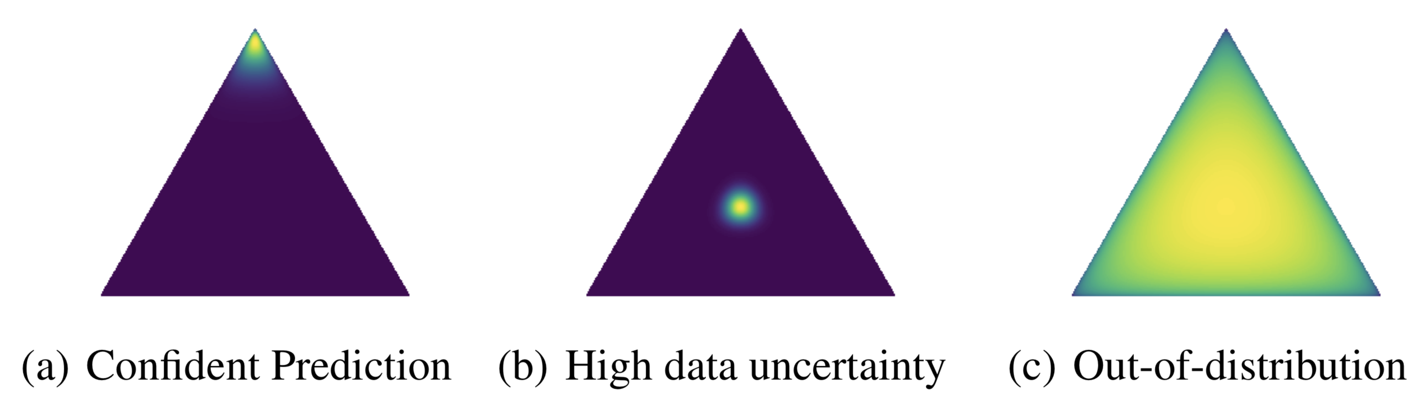
Figure 1: An exemplar 3 class simplex taken from a paper by Malinin & Gales (2018). This represents the optimal uncertainty behaviour of a classifier given various data points. The lighter colour refers to the probability of a class being placed in the particular area of the space.

When considering epistemic uncertainty this can again take multiple forms, these are known unknowns and unknown unknowns. As the names suggest, these are when the types of out-of-distribution data are known beforehand and when it is not. Unknown unknowns present a more challenging problem, as it is much more challenging to prepare the model for something that is unknown. Nevertheless, work in the field can help alleviate these uncertainties, and are predominantly discussed in section 2.1. Tangentially related fields such anomaly detection and adversarial defence also contribute to the discussion. Anomaly detection models look to identify inputs that do not fit into the distributions on which it were trained and adversarial defence models aim to identify inputs intended to deceive the model. Indeed, a lot of the work in the uncertainty calculation field compares against and shares ideas from these approaches when trying to address the graceful degradation problem. However, both of these methods might leverage information that would not be known. So when considering solutions to the graceful degradation problem it is important to consider which types of unknowns and uncertainties each method is addressing. It is also important to consider the data available to train the system and which supervision strategy is most appropriate during training.

1.4 Supervision Strategies

In machine learning there are a spectrum of supervision strategies with which a model can be trained. Supervision in machine learning refers to the error signals with which the model updates itself. In supervised learning a given input has a desired output, that is, it has a label. The learning process can be thought of as like a teacher supervising students. In unsupervised learning the model has no desired output, but rather its goal is to understand the underlying distribution within the data. There also exist intermediate approaches, such as semi-supervised approaches where the model is given a mixture of labelled and unlabelled data, allowing the model to apply pseudo-labels to the unlabelled inputs, depending on where it places a point in its distribution. A more recent approach to learning is self-supervised learning, a technique which has massively improved results in the domain of language models, as shown in a paper by Chen et al. (2020b). In the self-supervised paradigm the data itself supplies the label, that is the model is given an altered datapoint and it is asked to reconstruct it. This might be appropriately arranging segments of an image, or selecting a word for a missing part of a sentence.

Each of these techniques have their own benefits in the representations they allow the model to form. For example, a self-supervised pre-training approach may give a model a better understanding of the underlying data distribution and help it generalise when moving out of this distribution, as is discussed later in section 3.2. Fully supervised learning largely outperforms other supervision techniques when testing on a single dataset, as shown by the consistent performance of supervised learners in the ImageNet challenge, at the time of writing being led by Foret et al. (2020). So there are merits for all types of learning, explicit error signals can allow stronger learning of task specific features and a less structured learning process can allow for a more robust inductive bias outside of the training distribution. Hence, all supervision methods will be relevant when models begin to stray from their trained distributions, therefore various supervision strategies are applicable to the graceful degradation problem and will be considered throughout the survey.

1.5 Taxonomic View of the Problem

To help understand the different aspects to the graceful degradation problem, it will be beneficial to form a taxonomic view of it. This is shown in figure 2.

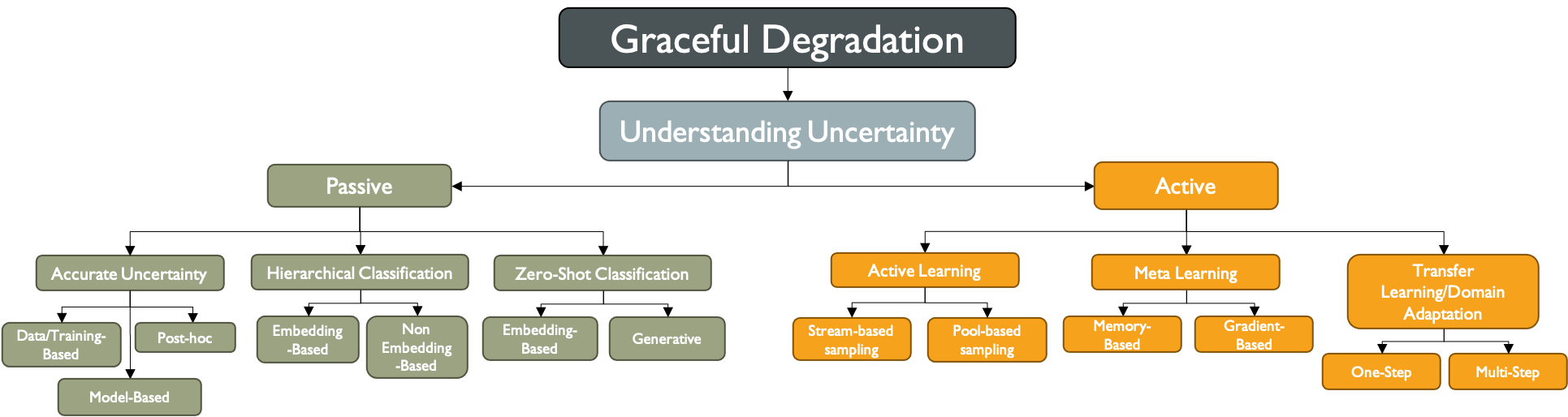
Figure 2: A taxonomic view of the graceful degradation problem.

Clearly all of the applications of graceful degradation stem from understanding uncertainty within the input space and are split according to how you deal with that uncertainty. Passive solutions are placed on the left hand side of the diagram and segregated into the three passive approaches to dealing with graceful degradation. Accurate uncertainties refers to the systems that notify an operator of their uncertainty and do not try to function on the data that is causing the uncertainty. This area has been split into three sections that further segregate these approaches, based on where the uncertainty calibration is sourced in relation to the machine learning pipeline. Then hierarchical classification is shown, along with zero-shot classification, which are also split into the different paradigms in the areas.

Active approaches are placed on the right hand side of the diagram, which are further split where appropriate. Meta-learning has been split into the memory-based and gradient-based approaches in few-shot learning. Furthermore, domain adaptation has been split into one-step and multi-step.

All of the splits in this taxonomy can be segregated further, but for the sake of brevity, these have been omitted from the diagram and will be discussed accordingly in subsequent sections. The remainder of the survey is outlined as follows. First passive approaches will be considered in section 2, then active approaches will be considered in section 3. Following these, a discussion will be presented in section 4, which draws comparisons between these two areas and where particular approaches might be the most appropriate. Finally, some conclusions and future work will be presented in section 5.

2 Passive Approaches

In the graceful degradation problem passive approaches can be considered as those that once trained are complete and require no additional changes to function optimally. Hence, these approaches are self-contained. They can broadly be split into 3 categories when considering the goal of the graceful degradation system and each refer to how they deal with uncertainty. There are those that output accurate uncertainties and express it to the operator without classifying. There are those that will attempt to classify data they are not explicitly trained on. Finally, there are those that will travel up the class hierarchy and offer a coarser-grained classification which they are more confident in. In this section, each approach will be discussed in more detail and notable papers will be highlighted.

2.1 Accurate Epistemic Uncertainties

As discussed in section 1.3, epistemic uncertainty is when the model is uncertain due to a lack of knowledge. That is, the model is uncertain on a classification because the data presented to it is outside of the distribution on which it was trained. Hence, epistemic uncertainties and obtaining accurate estimations of them is very relevant to the graceful degradation problem. This is particularly true when communicating to an operator about the certainty of its output and when it may be necessary for the operator to take control of the classification process. For this reason, methods of obtaining accurate uncertainties will be analysed first.

When considering information outside of the source distribution the type of unknowns need to be considered, for considering known unknowns will prompt different solutions to unknown unknowns. Therefore, throughout the breakdown of tools to calculate epistemic uncertainty, the type of unknowns each tool operates on will be discussed. Out-of-distribution detection models also fit into this category of models as they aim to achieve similar functionality.

In obtaining epistemic uncertainties the field can be broadly split into 3 sections that are defined by the machine learning pipeline: Data/training-based, model-based, and post-hoc. In data/training-based methods you look towards the data in obtaining representations that can produce accurate uncertainties where necessary. In model-based methods the uncertainty framework is built into the architecture of the model itself. Finally, in post-hoc approaches the uncertainty is calibrated by applying the methodology to the output of the model. There also exist hybrid methods, indeed many of the methods at the state-of-the-art employ strategies that utilise ideas from more than one of these sections. However, in segregating and understanding the area these categories logically distribute the approaches in the field and help develop an intuition.

2.1.1 Data/Training-based

In this category of methods the uncertainties are calibrated using additional data to that which the model is trained on. This might be in a supervised manner or an unsupervised manner (Winkens et al. (2020), Yu & Aizawa (2019)). Some papers analyse the distribution of data in the representation space in order to understand predictive uncertainty (Ramalho & Miranda (2019), Kamoi & Kobayashi (2020)). Furthermore, another paper by Kurakin et al. (2017) shows that adversarial examples can persist in the real world even when printed and reprocessed. Hence, data is at the heart of the uncertainty estimation problem, this data can be generated (Sensoy et al. (2018),Lee et al. (2018a), Lee et al. (2018b)), perturbed (Hafner et al. (2020)), or it might come from additional datasets (Li & Hoiem (2020)). Here, a leading method which takes the former approach will be discussed.

Sensoy et al. (2020) present method that creates uncertainty aware deep classifiers by using generative models to create out-of-distribution samples. The presented approach uses the output of a neural network to model a Dirichlet distribution, representing a probability distribution over possible classes. This distribution is then used to estimate the uncertainty for a given classification. Out-of-distribution samples are then generated using a variational auto-encoder), the generator being trained to perturb the latent representations for given samples. Two discriminators are trained: One to be fooled, ensuring the representations are sufficiently perturbed; and another which is not fooled, ensuring semantic similarity is preserved. The classification model is then trained on the out-of-distribution samples, as well as the underlying dataset. The effect on class uncertainty is shown in figure 3, where blue and red represent low and high uncertainty, respectively. It is clear the proposed approach (d), recognises the underlying distribution of the classes and takes that into account when classifying data.

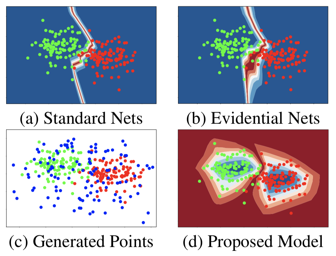
Figure 3: A figure taken from the paper by Sensoy et al. (2020). In (a) and (b) standard approaches in the field are shown, and the uncertainties are shown near class boundaries. In (c) generated points are presented on which the model can train, and in (d) the class boundary of the proposed model is shown. In (a), (b), and (d) blue refers to highly certain, and red highly uncertain.

The authors evaluate their approach by training it on a dataset with half of the classes held out, it was then tested on a mixture of seen and unseen classes. The key evaluation measure in this procedure are cumulative entropy graphs, namely the area underneath them. Total uncertainty thus high entropy, would be expected on the unseen examples. On seen examples, high entropy should be desired only on the incorrectly labelled samples. This was reflected in their results, which can be seen later in figure 5a and b. This method explores both aleatoric and epistemic uncertainties, hence considering known unknowns and unknown unknowns. Unknown unknowns could be better analysed by passing the model data from a different dataset entirely, such as using fashion-MNIST on a model trained on MNIST, this is something done in a paper by Charpentier et al. (2020) discussed in section 2.1.3. However, this is a good example of how extra data can be leveraged in uncertainty estimation and presents a model that is effective in accurately expressing uncertainty in the graceful degradation problem. Moving along the machine learning pipeline, model-based approaches will be discussed.

2.1.2 Model-based

In model-based approaches the uncertainty is built into the architecture of the model and is generated intrinsically. Such approaches can take distributions over the model parameters like in bayesian neural networks, or they might leverage other information such as that from gradients to evaluate uncertainty.

In bayesian frameworks the uncertainty between the training and test distribution are considered to arise from uncertainties in the model itself. To instantiate one of these systems using a neural network you apply a probability distribution over all of the parameters of the network, hence removing the deterministic nature of a forward pass. The inference process in bayesian neural networks involves a number of forward passes, thus allowing the weight uncertainties to propagate through the network and giving a probability distribution for the output. These can be sampled in a variety of ways the most popular of which being variational inference, a technique popularised by Blundell et al. (2015) where Bayes by Backprop was introduced. This method would catalyse the development of the variational approach as it showed backpropagation could work as intended when training these probabilistic networks, something which previously presented a significant challenge to the field.

Lots of the work in the bayesian network space has expanded on this, such as obtaining weight uncertainties implicitly using hypernetworks Pawlowski et al. (2018), or by viewing dropout as a form of bayesian inference Gal & Ghahramani (2016). Another paper by Tran et al. (2019a) restricts the bayesian properties to single layers to analyse uncertainty. Here we will highlight the hypernetwork approach. However, the reader can find an implementation orientated review of bayesian approaches in a recent survey by Jospin et al. (2020) and a more comprehensive view on uncertainty quantification in another by Abdar et al. (2020).

Hypernetworks, first presented in a paper of the same name by Ha et al. (2016), are a method of using a neural network to generate the weights for a target neural network. Pawlowski et al. (2018) utilise hypernetworks to obtain implicit distributions of weights, such distributions have intractable probability densities but allow for very easy sampling. The authors sample from the weight distributions given by the hypernetworks during a forward pass. This is reflected in figure 4a, where the hypernetwork $G$ produces a weight distribution for the second layer of weights in the main network. The predictive uncertainty in the model is also reflected using a toy regression task, shown in figure 4b. This shows their method exhibits the best trade-off between regression accuracy and predictive uncertainty, when compared to other methods in the field.

(a)

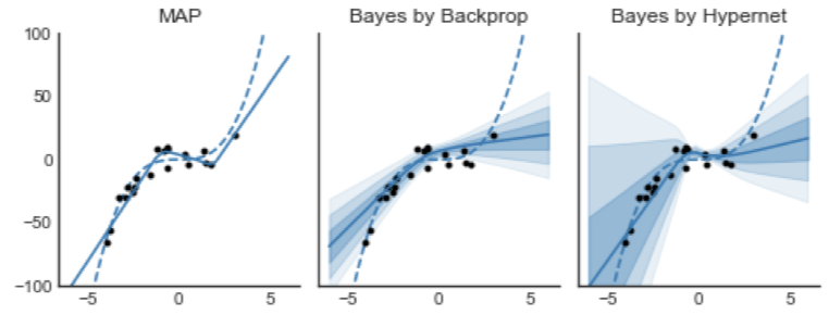
(b)

Figure 4: In (a) the interaction between the hypernetwork and the main network is shown, with the hypernetwork producing the weight distributions for the second layer of the main network. In (b) the effect on model uncertainty is shown on a regression task for 3 different models. Maximum a posteriori (MAP), Bayes by Backprop (Blundell et al. (2015)), and the hypernet approach (Pawlowski et al. (2018)) here the lighter shade of blue refers to a higher uncertainty, the blue dashed line refers to the ground truth, and the solid line the prediction of the model.

To train this system the hypernetwork generating the weights needs to be optimised, they do this through a method that closely resembles adversarial training. A generator models the variational distribution of the main network, a discriminator then approximates a density ratio between model parameters given those of the generator, and the probability of generator parameters. The authors show this information allows them to effectively approximate the evidence lower bound (ELBO), something used to optimise bayesian neural networks in the field.

As part of the analysis the main network is tested on in-distribution images and out-of-distribution images to analyse the generalisability of the method and its uncertainty awareness. The performance is quantified on these distributions by using the area under cumulative density plots of entropy. This is the same analysis as that in the paper by Sensoy et al. (2020), examples of which are shown in figure 5a and b. Here it is named the area under curve (AUC), not to be confused with the area under the receiver operator curve, which is the area under the curve of true positive rate against false positive rate and generally called the AUC.

The argument for using this form of analysis is that if the model is confident in its prediction, as in the in-distribution case, the AUC should be high as the entropy will more frequently be a low value, shown in figure 5a. Whereas in the low confidence out-of-distribution case, the entropy should be low until close to the maximum entropy value, shown in figure 5b. The method outperforms all other competing methods in both maximising the in-distribution AUC and minimising that on out-of-distribution data.

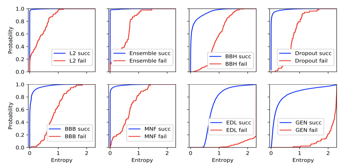
(a)

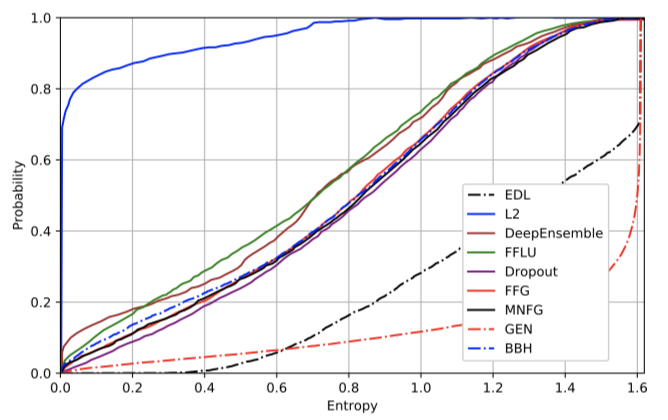
(b)

Figure 5: Two figures taken from the paper by Sensoy et al. (2020), showing cumulative density plots of entropy. In (a) correct and incorrect distributions are compared are compared for various uncertainty aware approaches. In (b) the distributions are shown for when they encounter out-of-distribution data. In both Sensoy et al. (2020) and Pawlowski et al. (2018) the area underneath these plots is used as a form of analysis.

The key advantage of the method is its flexibility and scalability, as the use of hypernetworks to generate the weights implicitly accounts for the architectural complexity of the main network. This allows the method to scale to very large and complex networks, something intractable in competing bayesian approaches. Hence, if the underlying classification problem is one that requires the representational capacity of a larger, more complex network, this method will suitably provide uncertainty measures for the problem. However, the authors only consider known unknowns in their analysis. That is, data semantically similar to that which it was trained on. Hence, this method may not be suitable when the model is likely to encounter data far outside of the training domain: Unknown unknowns. The authors could have undertaken such analysis, however, the authors do test their method on adversarial samples and show it performs better than competing bayesian approaches. Another recent approach also uses hypernetworks when identifying out-of-distribution samples, which is presented in a paper by Ratzlaff & Fuxin (2020).

There have been a number of papers that use non-bayesian approaches to this problem. Here the uncertainty can be calculated using signals from the model itself, this might be gradient information, as in a paper by Oberdiek et al. (2018), or using ensembles as in a paper by Kachman et al. (2019). Furthermore, a paper by Hein et al. (2019) analyses the ReLU activation function in neural network design, proving it can aggravate out-of-distribution errors. An interesting non-bayesian approach is presented in a paper by Geifman et al. (2019), where the authors suggest highly confident predictions are an artefact of dynamic and stochastic training processes. The paper suggests uncertainty signals obtained from models which are optimised on a classification problem will be inherently biased towards making predictions with high confidence. It is argued this is a form of overfitting which prompts sub-optimal behaviour on out-of-distribution samples and that the stochastic gradient descent process deforms reliable confidence estimates throughout the training process.

To address this, more accurate readings of predictive uncertainty can be obtained from earlier snapshots of the network. To do this, weights from earlier iterations of the network are sampled to give accurate estimates for uncertainty. Two methods of obtaining these weights are proposed. One trains an input-wise selection mechanism to identify earlier iterations of the model which improve the uncertainty estimation, this method requiring an auxiliary dataset. The second method looks to approximate the first method without the use of an auxiliary set, this has the benefit of shorter training periods in the model at the cost of longer inference times. This second method, which leverages the fact that easier samples are learned earlier on in the training process, performs surprisingly well and is used for the majority of their analysis. The method outperformed all competing methods at the time, when maximising the confidence score of correct predictions. The analysis fails to include out-of-distribution samples, hence only aleatoric uncertainty is considered. However, the method performs well and is a good example of a model-based approach to the uncertainty estimation problem, if not explicitly used in the graceful degradation setting. Now the focus will be shifted towards the end of the machine learning pipeline in post-hoc methods.

2.1.3 Post-hoc

In post-hoc approaches you focus on the output of the model and use it to calibrate the predictive uncertainty. The benefit of these approaches is that they can often be incorporated with any architecture and arguably any machine learning model. These methods look to transform the output so that it more accurately reflects the confidence of the prediction, this might be through simple temperature scaling or use more complicated measures like in a recent paper by Kull et al. (2019) which utilises Dirichlet distributions. Other recent methods include knowledge distillation of uncertainties (Pouransari & Tuzel (2020)), utilising likelihood ratios (Ren et al. (2019)), or minimising KL divergence between OOD samples and a uniform distribution (Lee et al. (2018a)).

A particularly relevant post-hoc approach explicitly calibrates their model on out-of-distribution datasets, presented in a recent paper by Shao et al. (2020). The authors incorporate an auxiliary classifier to the post-hoc framework that identifies mis-classification. The classifier is a simple neural network which maps the model output to a calibrated soft-max, which can be used to give more appropriate confidence estimates. An auxiliary class is also introduced which identifies miss-classified samples and is used to calculate the confidence of a given classification. Two strategies of doing this are developed, one where the auxiliary classifier has an output neuron for every class and an additional one for the auxiliary class. The second method simply temperature scales the output of the model and the auxiliary classifier has a single output which predicts the classification accuracy. These are shown in figure 6a and figure 6b respectively in a figure taken from the paper. The auxiliary classifier was trained in a supervised manner, aiming to map the class of incorrect classifications to the auxiliary class.

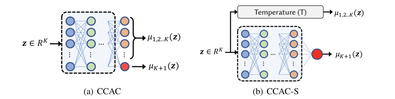
Figure 6: A figure from the paper by Shao et al. (2020) the authors depict their two approaches, with the soft-max logits $\bf{z}$ being taken as an input, and the approach outputs a calibrated soft-max. The two approaches are compared, the complete version in (a) and the simplified version in (b).

The models were trained on the CIFAR-10 dataset and tested using a modified CIFAR-10 dataset, which was synthesised using CIFAR-100 classes. It included some some semantically similar classes from CIFAR-100 which were mapped to the similar class in the CIFAR-10 set, representing known unknowns. Unknown unknowns were analysed by including completely out-of-distribution samples, represented using classes that were not semantically similar. The method was able to accurately identify known samples with high confidence, record low confidence in incorrect predictions, and would consistently use the auxiliary class when encountering out-of-distribution data. Hence, this is very relevant in the graceful degradation problem in that the model performs optimally when leaving the distribution on which it was trained. This is shown both close to the distribution and well outside of the distribution. The analysis shown in this paper is perhaps the best and most practical analysis to perform when analysing graceful degradation problems. The method does necessitate the training of the auxiliary classifier which can be expensive, but there it is very flexible regarding the architectures on which it can be used.

Another similar method at the state-of-the-art is Posterior Networks proposed in a paper by Charpentier et al. (2020). The authors propose a neural network which uses normalising flows to predict an individual closed-from posterior distribution over probabilities for a given input sample. It is comprised of 3 components, an encoder which maps inputs to a latent position, a normalising flow which provides density estimations for each class in the latent space, and a bayesian loss which allows for uncertainty aware training. This is shown in figure 7. The key problem solved in this paper is that the method is designed to work without the knowledge of known unknowns and does not leverage any additional data.

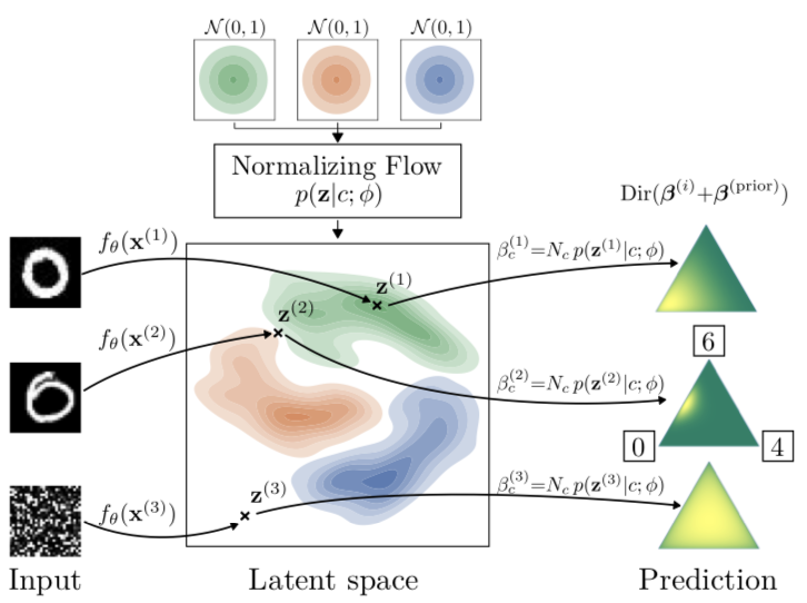
Figure 7: A graphical representation of the model in the paper by Charpentier et al. (2020) taken from the same paper. The inputs are mapped to a latent space, the densities within this space are morphed by normalising flows. Predictions for various inputs are sampled from this space and shown in simplexes. For the sake of intuition, only 3 classes are shown in the simplex examples.

The method is evaluated on in-distribution samples and out-of-distribution samples for both known unknowns and unknown unknowns. This can be also seen in figure 7. Furthermore the predictive uncertainties are reflected in the simplex diagrams to the right hand side, matching those in figure 1. The training datasets included CIFAR-10 and MNIST. The predictive uncertainty was evaluated on unseen datasets, left-out classes, out-of-domain, and on dataset shifts. State-of-the-art results were achieved in all areas and is very relevant and successful in the graceful degradation problem of communicating uncertainty. Rather than expressing uncertainty upon leaving the data distribution, it may be more desirable for the model to function in the encountered domain instead, this is where zero-shot learning could provide insights.

2.2 Zero-Shot Classification

In the field of zero-shot learning the goal is to design models that can classify data it has never seen explicit examples of. Hence, this area is about the model understanding the space outside of what it knows and performing well in this area. This technique clearly only works on known unknowns, but it will be beneficial to discuss zero-shot learning techniques in the context of the graceful degradation where known unknowns exist.

In zero-shot classification there exist two main protocols: Conventional zero-shot learning and generalised zero-shot learning (GZSL). These methods differ in their targeted test distributions. In conventional zero-shot learning the test distribution is only the data on which zero-shot classification should be achieved. In GZSL the test set will include both classes from the training distribution and novel classes on which the model should achieve zero-shot classification. The latter is arguably the most relevant in the graceful degradation problem, as a gracefully degrading system should also perform optimally on the trained distribution. Hence, some papers from this area will be considered. Zero-shot learning has also been used in other vision tasks, namely semantic segmentation, recently shown in a paper by Bucher et al. (2019).

In GZSL the goal is often to define a shared embedding space on which the seen and unseen classes can develop discriminatory representations. The embeddings for the unseen classes are often formed using additional semantic information. These might be in the form of attributes (Farhadi et al. (2009), Liu et al. (2020), Huynh & Elhamifar (2020)), word embeddings (Mikolov et al. (2013), Norouzi et al. (2014), Sariyildiz & Cinbis (2019)), textual descriptions (Reed et al. (2016), Elhoseiny & Elfeki (2019)), or might employ generative techniques (Yu et al. (2020), Han et al. (2020), Ni et al. (2019), Sariyildiz & Cinbis (2019)). One recent implementation in a paper by Wu et al. (2020) uses self-supervision to learn domain-aware features in the GZSL task, something that may also be relevant in domain adaptation which is discussed in section 3.2. As an example, GZSL systems be applicable in drone systems that need to classify objects which only have semantic descriptions, like in the first vignette.

The authors of Keshari et al. (2020) propose that one of the primary reasons GZSL systems fail is because they are required to classify hard samples of unseen classes at test time. That is, the samples are close to another class, thus causing confusion in the classifier. To that end, the authors of the paper propose a new attribute based methodology of training GZSL systems, whereby they train the model given an over-complete distribution of samples. In the proposed methodology, an over-complete distribution is one that aims to improve the generalisability with the respect to the unseen classes. This is done by generating examples of the unseen class that are close to the distributions of seen classes, hence producing an extended boundary for the unseen class. This allows the model to generalise better when seeing the real instances of the class. The resultant effect on class embeddings can be seen in figure 8a, where all possible hard samples are generated relative to each class.

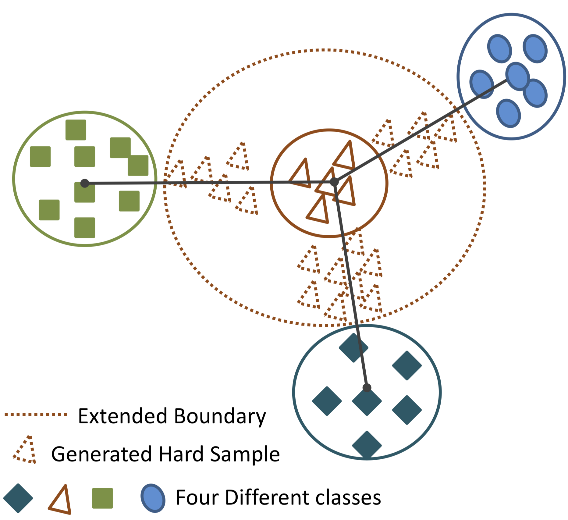
(a)

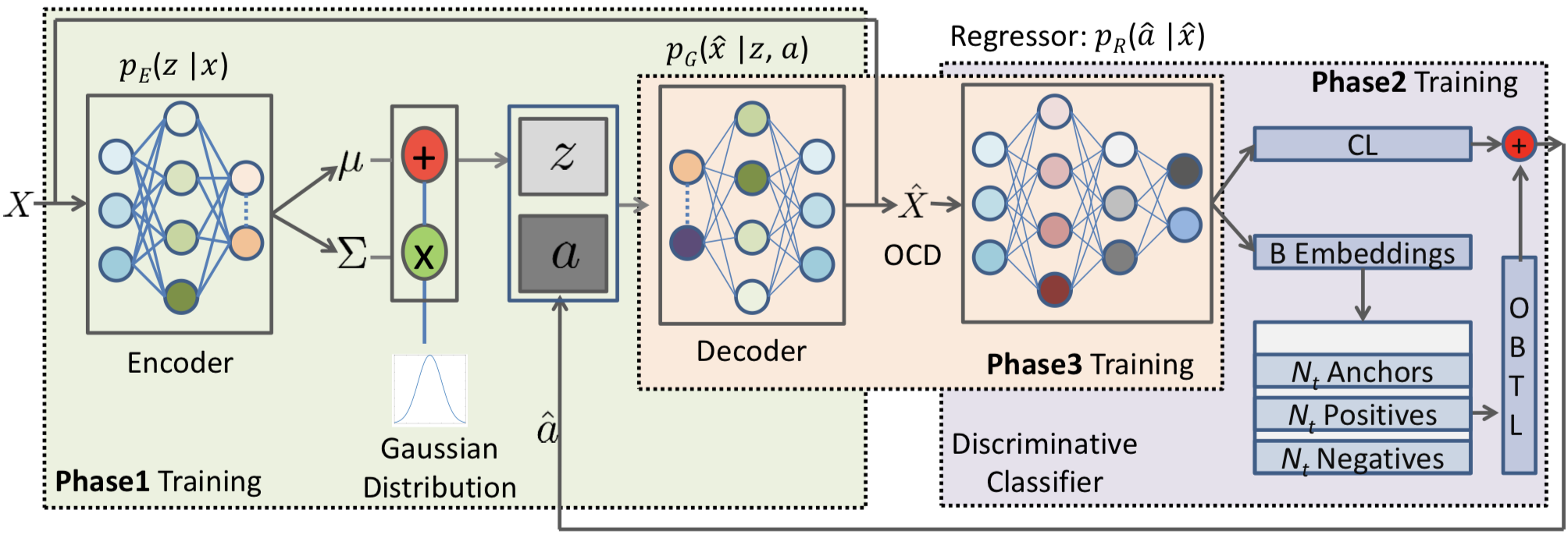
(b)

Figure 8: Two figures taken from the paper by Keshari et al. (2020). In (a) the process of generating over-complete samples is shown with relation to the class space, and how it creates an extended boundary by producing hard samples. In (b) the model structure is shown in its various components and how each of those relate to phase of training.

Figure 8b demonstrates the structure of the approach. The model works by first mapping inputs $x$ to a latent position $z$ using an encoder, a decoder then generates samples $\hat{x}$ given the latent encoding $z$ and attributes $a$. The encoder and decoder combination are known as a conditional variational auto-encoder (CVAE), in this instance it is conditioned on the attributes of the inputs. Finally, a regressor maps the samples $\hat{x}$ to their predicted attributes $\hat{a}$ and is optimised using an online batch triplet loss (OBTL) and a centre loss (CL). The OBTL ensures high inter-class separability and low intra-class separability, and the CL ensures that the generated points for a given class keep the distribution centred about its learned centre.

The model is trained in 3 phases, which can also be seen in figure 8b. In the first phase the CVAE is trained on seen data to produce a latent position $z$ given $x$, which is subsequently appended to the attributes of the data point, $a$, creating a vector $[z,a]$. This is used to create the generated samples $\hat{x}$ and is trained using KL divergence and conditional marginal likelihood. The trained CVAE should be able to generate synthetic data given attributes $a$. In the second phase of training the regressor/classifier is trained using the OBTL and CL to optimally map synthetic data to corresponding attributes. The third phase of training regularises the over-complete distribution to ensure it creates class specific examples even when randomly sampling from the embedding space. The authors find their model would outperform most existing approaches on common ZSL datasets: Animals with Attributes 2 (AWA2)(Lampert et al. (2013)), Caltech-UCSD Birds (CUB) (Wah et al. (2011)), and SUN (Scene UNderstanding) (Patterson & Hays (2012)).

A recent implementation by Liu et al. (2020) approaches the zero-shot learning problem in a way that reflects the hierarchy of classes and uses word embeddings to do so. Zero-shot learning techniques typically use euclidean embedding spaces, in this paper the authors project each sample to a hyperbolic embedding space, the first example of such an approach in zero-shot learning. The embedding space used is the same as that in a paper by Nickel & Kiela (2017), a Poincaré hyperbolic space. This allows hierarchical representations in the input space and the distances within it are differentiable. The framework of their approach has two components, shown in figure 9a, a figure taken from the paper.

The first of these components is the learning of a hyperbolic label embedding which embeds image labels into a hyperbolic space, encoding hierarchical information as well as semantic information in doing so. Poincaré embeddings are used to encode WordNet noun hierarchies into what is known as a Poincaré ball, a disk in Poincaré space where the distance scales exponentially as the edge of the disk is approached. This prevents hierarchical representations from becoming increasingly clustered as the edges are made, allowing the embeddings to learn the hierarchical connections of WordNet whilst preserving the semantical distances between the words themselves. The authors also employ GloVe word embeddings to capture semantical relationships between classes, this also being trained in a Poincaré ball space. This produces two embeddings which are concatenated to form a single embedding for image labels which has structural and semantical information encoded within it.

The second component in their approach is the learning of image embeddings, this process consists of two components: An exponential map, which projects image features into the hyperbolic space; and a transformation network which learns to align the new image representations with their respective labels in the hyperbolic space. The resultant system is one that transforms image embeddings into a shared hyperbolic space with the word embeddings, meaning both hierarchical and semantic relationships can be learnt in visual representations. Such a hierarchy can be seen in figure 9b, another figure from the paper. The model was trained to minimise the distance between the image embeddings and the label embeddings.

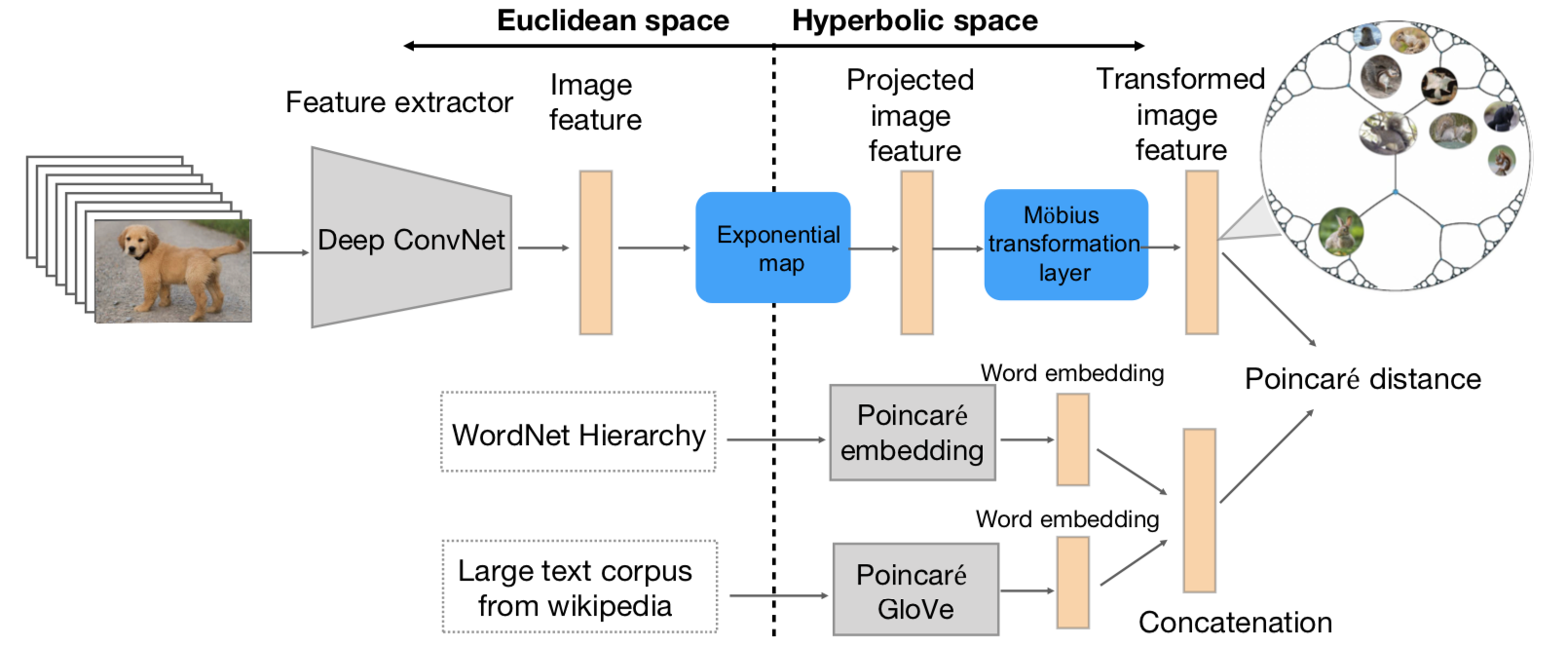
(a)

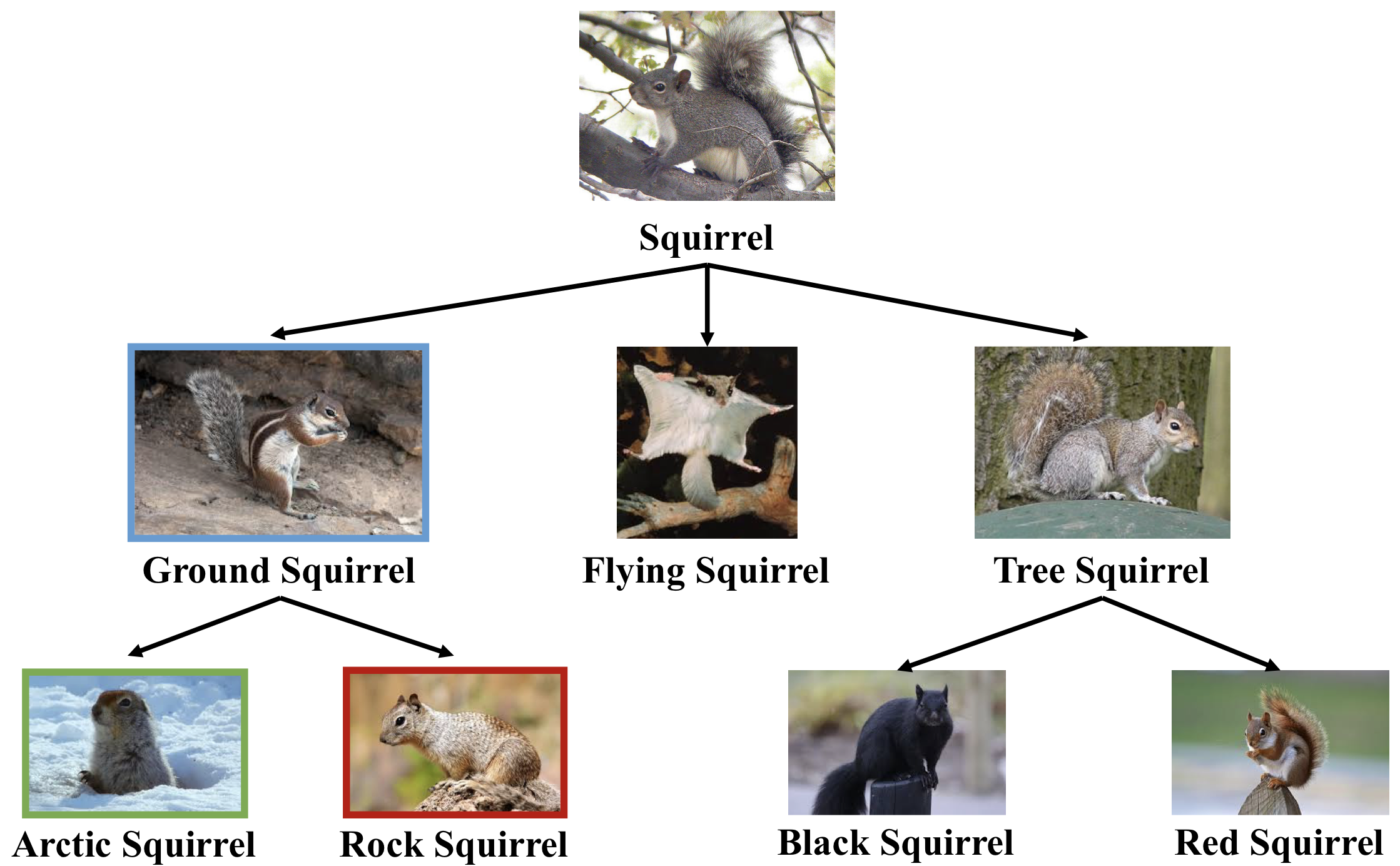
(b)

Figure 9: Two figures taken from the paper by Liu et al. (2020). In (a) the structure of the proposed approach is presented. In (b) the hierarchy of a given class is shown, in this case squirrels.

Experiments were conducted on ImageNet (Deng et al. (2009)), a popular benchmark in the ZSL community. The unseen classes are segregated by the number of connections they are away from a seen class, making 3 different test sets: 2-hop, 3-hop, and All. The model is evaluated on all three of these test sets, both in the ZSL and GZSL paradigms. The model, whilst not achieving perfect top-1 accuracy in classifying unseen classes, would correctly output the parent class in many cases. That is, the model would often include a label further up the class hierarchy as opposed to another fine grained prediction. Arguably this ability to predict the immediate parent class of a model reflects robustness in a ZSL model, as it shows an understanding of the class space. Furthermore, such hierarchical predictions make systems more applicable in real world scenarios, particularly in the graceful degradation setting where an operator would prefer a confident coarse-level prediction, than a single low confidence fine-level label. Indeed, such approaches will be discussed in the next section.

Zero-shot learning approaches are relevant in the graceful degradation problem as the models aim to understand the space outside of the seen classes and looks to be better prepared as they approach these distributions. These models necessitate the existence of known unknowns, limiting their applicability. However, there are an abundance of datasets that can help facilitate the training of such systems. Although it is not explicitly discussed, it is clear such systems overcome epistemic uncertainty in making predictions, as they classify data outside of the training distribution. Although, zero-shot learning techniques often lack reliable confidence estimates and as such will not be applicable to fully autonomous systems where high error rates are not permitted, let alone over-confident errors. A way around the high error rate of these systems is to produce hierarchical outputs, like in the previous approach. More explicit investigations of hierarchical classification have been undertaken in the field and will be discussed in the next section.

2.3 Hierarchical Classification

In the hierarchical classification problem, rather than asking the model to make a prediction in an area in which it is uncertain, the model is instead asked to predict a parent class at a level of hierarchy at which the it is more confident. For example, if the model failed to recognise an animal as a pigeon it might be able to recognise that the animal is a bird and offer a range of classes the bird might fit into. This can be seen as a compromise between the other passive approaches to the graceful degradation problem: The image is not classified due to uncertainties, but more information is offered as opposed to simply returning an uncertainty.

Like in the aforementioned paper by Liu et al. (2020), recent investigations into hyperbolic embedding spaces (Khrulkov et al. (2020), Chami et al. (2019)) have proven to be particularly insightful in the hierarchical labelling problem (López & Strube (2020), Dhall et al. (2020)). However, such investigations have been more recent and there is a wealth of existing literature in hierarchical image classification that takes more conventional approaches. These can broadly be split into embedding-based approaches (Faghri et al. (2017), Grassa et al. (2020), Seo & shik Shin (2019), Koo et al. (2019), Guo et al. (2018)) and non-embedding based approaches (Bertinetto et al. (2020), k. Nakano et al. (2017), Kumar & Zheng (2017), Chen et al. (2018), Deng et al. (2014)), which typically exploit label hierarchies. Another interesting approach by Cha et al. (2020) takes the superclass label as an input to help the fine-grained classification. Furthermore, hierarchical labels were also implemented in an active learning paper by Nakano et al. (2020). Active learning approaches will be considered in section 3.1, but this shows the relationships between the various avenues of the graceful degradation problem. To give context, hierarchical labels might be used in a disaster response system where it cannot classify a particular object, but it might be able to classify it as potentially endangering to, or holding, survivors .

A particularly relevant technique in this area is presented in a paper by Achddou et al. (2020), where a new type of learning is proposed, nested learning. In this paradigm the model should understand the hierarchical nature of the input and provide information of varying specificity depending on the data sample. This allows the model to output confidence levels for classes at different levels of granularity, including the fine-grained class. The core work in the paper discusses and formulates such learning problems and it is shown that systems trained in such a manner can offer meaningful coarse-level predictions even when the fine-level predictions are severely degraded.

Four main components are designed to make such systems work: A sequence of low dimensional nested representations, calibrated output predictions, the combination of nested predictions, and a practical and stable training protocol. The process of extracting nested representations is shown in figure 10 where by the input $X$ learns information about the coarse label $\hat{Y}$ through the classification using $f_{1}$ and uses this to inform the following label at the next classification layer. Between these classification layers the input is compressed sequentially but skipped connections also allow information to flow between the layers. The second step involves learning complementary information that when combined with output of a coarse classification layer, $f_{n}$, can provide meaningful insights to classification at $f_{n+1}$. Here the skipped connections are necessary to prevent the input from being degraded through when coarse level predictions. The score outputs need to be calibrated as a soft-max of a given class at layer $f_{n}$ does not necessarily equate directly to its probability. This is because at a given coarse-level classification, the number of classes available is no longer equal to all of the classes across all layers, hence they need to be re-normalised. Finally, the authors train their model in a cascaded manner, gradually adding finer level classes iteratively as the coarser predictions are optimised, thus optimising deeper parameters as training goes on.

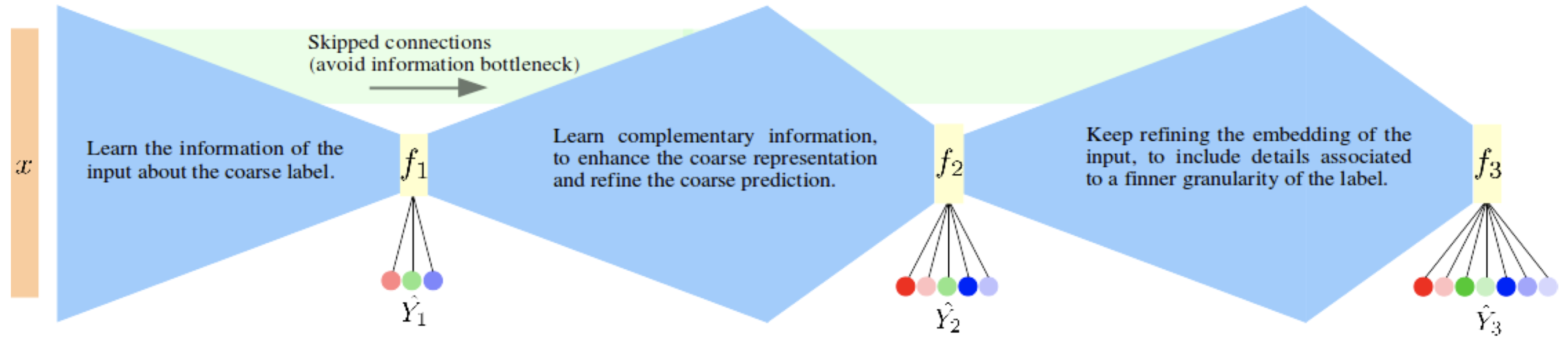
Figure 10: A figure taken from the paper by Achddou et al. (2020) presenting the structure of the approach.

To evaluate their method a number of datasets were used to train the models, including Fashion-MNIST, CIFAR-10, and CIFAR-100. The latter dataset has an accompanied taxonomy, the former had such taxonomies manufactured by the authors. Results suggest that coarsely annotated data would allow for more robust and less over-confident fine-level predictions. Furthermore, given a specific training budget, the proposed approach still outperforms a typical end-to-end approach. When given adversarial examples the approach still showed robustness and a reduced over-confidence. The authors fail to include state-of-the-art papers in their comparison, opting instead for an end to end version of the same architecture, whilst this does highlight the benefits of the approach, it does not show the effectiveness of it in the context of the field. Something also neglected in the analysis is out-of-distribution samples, whether or not the nearest parent label can be identified by such models would be an interesting analysis. So whilst the authors do not explicitly investigate the graceful degradation problem, they do investigate tangentially related areas such as adversarial defence and uncertainty in classification. Furthermore, the paper does suggest an uncertainty-centric method, that provides such estimations at varying levels in the class hierarchy. This is something desirable in graceful degradation, albeit in this instance limited to the aleatoric case. Furthermore, it is clear such methods compliment branched neural network structures due to the hierarchical nature of the output branches, indeed such structures have recently been shown to allow for greater adversarial robustness, efficiency, and accuracy in a recent publication by Hu et al. (2020).

Hierarchical methods such as these could prove promising in the graceful degradation field, a model understanding uncertainty throughout the class space at varying levels of granularity will allow models to provide more specificity when giving low confidence predictions. It will also allow more specificity when suggesting additional information is needed. Requesting additional information and retraining is something outside of the remit of passive methods and is something that active approaches look to do, these will be discussed in the following sections.

3 Active Approaches

In this category of approaches, rather than the system being self-contained and complete, it has the option to adapt as the input landscape evolves. That is, to function optimally an adaptive learning model will reconfigure itself when encountering uncertainty. Here, three splits are identified, each defining a different magnitude of reconfiguration. In active learning the reconfiguration occurs in an input-wise fashion, whereby individual data points are selected to inform model updates. In the graceful degradation scenario this might be after the model has been deployed and operate in a manner akin to lifelong or continual learning, hence both will be discussed in this area. These approaches might be applied when encountering a new object within a known domain. The second area is that of domain adaptation where the model is trained on a distribution of data and then asked to operate on a different distribution of data. This might be relevant when a models task does not change but its environment does, like a disaster response drone moving to a new landscape. Hence the model is retrained to fulfil its purpose in the new environment. Finally, in meta-learning the feature space of the model will change and the model is encountering objects that are different to that on which it was trained. Hence, retraining is necessary if the model is to be of any use. Such techniques might be applicable when a smart city system is applied to a new city or area and is required to help assist in new/different events.

3.1 Active and Continual Learning

In this category of approaches the models will be updated using smaller reconfigurations, such updates might be needed when seeing a particular data point which causes uncertainty in the model, like a peculiar situation for a smart city system or a particular object in a disaster response drone. Here the operator can label a particular datapoint for the model to update itself. This might update the systems knowledge of the distribution as in the active learning case, or it might begin to give the system knowledge of a new task as in continual/lifelong learning. The important distinction here is that it happens with a small number of data points, as opposed to entire distributions.

In an ideal scenario unconfident samples would be continuously labelled by the operator in a continuous manner, as in continual learning. In this field the system is faced with a continuous stream of data to learn from. A popular paradigm in this field is the online setting, where the data is passed through once and the system is required to incrementally build its knowledge of the problem. The approaches to continual learning often focus on alleviating the catastrophic forgetting problem and can be split into three categories: Regularisation-based, memory-based, and model-based. Regularisation-based approaches impose constraints on the weight updates of the model (KJ & Nallure Balasubramanian (2020), Jung et al. (2020), Mirzadeh et al. (2020)), memory-based methods centre the approach on memorable examples in the data space (van de Ven et al. (2020), Cong et al. (2020), Pan et al. (2020), Ke et al. (2020)), and model-based approaches change the architecture of the model to handle new information (Singh et al. (2020), Mallya & Lazebnik (2018)). A recent paper by Caccia et al. (2020) presents a novel approach that focusses on solving unseen out-of-distribution tasks. A paper by van de Ven & Tolias (2019) presents an interesting breakdown of the applications of a continual learning system, whereby the system either has to classify an item if given a task, classify an item according to a distribution tasks, or classify both the item and the task it belongs to.

In a deployed system all three of these scenarios could be consistent with an active gracefully degrading system. In this scenario continual learning could be implemented to gradually build a models understanding of the task spaces and data distributions within them, by continuously providing labels for low confidence classifications due to out-of-distribution errors. However, this might not always be feasible and is counterintuitive as the system is in place to automate the classification process, so it may be beneficial to also review the field of active learning.

In modern machine learning problems annotated data is often a luxury that takes a great deal of time to produce, therefore obtaining usefully annotated data quickly will be important. In active learning, the goal of the algorithm is often to choose data that will most appropriately separate the classes and suggests that it be annotated. The two most popular paradigms in the active learning field are pool-based sampling and stream based sampling.

In stream-based sampling, inputs are continuously given to the model and it is is asked whether to request for a label from the oracle or label the point itself, which bears some similarities to continual learning. Some recent approaches in this area include a paper by Shah & Manwani (2020) where an option to reject classification is included and a paper by Murugesan & Carbonell (2017) where an ensemble-esque approach is taken. Other recent work includes that by Fujii & Kashima (2016) and Hong & Chae (2020).

Pool-based sampling presents a pool of unlabelled images to the model and supplies a corresponding annotation budget with which to optimally consult the oracle for annotations. It first trains on the samples allocated to it randomly, the model then classifies the remainder of the pool. The samples with the lowest confidence are then selected for annotation by the oracle, moving them to the training set. The process is repeated until test performance on a test set is sufficiently high. There are two methods of selecting samples for labelling: Singleton labelling where single points are chosen for annotation (Yang & Loog (2018), Beluch et al. (2018)) and batch labelling where a batch of points are selected for annotation (Ash et al. (2019), Yoo & Kweon (2019), Shi & Yu (2019)). Recent papers by Sinha et al. (2019) and Tran et al. (2019b) take variational and bayesian approaches respectively, methods also discussed in section 2.1. Selecting samples individually can often be wasteful of resources, hence more recent progression has concentrated on the batch-based approach.

In deployed machine learning systems the oracle will refer to an operator and the system may desire manual annotation when it encounters an object it has difficulty classifying confidently. This might refer to the first vignette, whereby the model asks the operator to label an object that falls outside of the trained distribution, thereby allowing to the model to informatively update its understanding of that area of the distribution.

In active learning the most important measure in this problem is how samples are chosen to be annotated, a common metric for this is confidence, as discussed in section 1.3 there are a variety of ways to do this. However, if a sample lies close to a class boundary and is miss-classified, minimising uncertainty in that prediction will inject error into the model. Since in the active learning scenario the model is not to know it is incorrectly classified, only that it is not confident in its prediction. Now increasing the confidence in that same prediction by picking a different label for annotation will improve the active learning loss function, but compound the underlying error on the uncertain label. This concept is explored in a recent paper by Aljundi et al. (2020). A figure from the paper illustrating this issue is shown in figure 11.

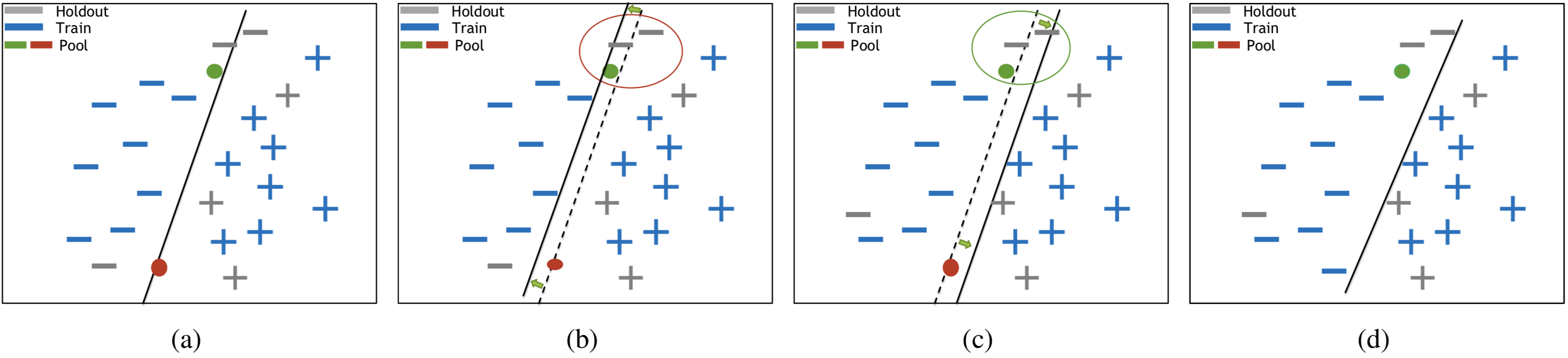
Figure 11: A figure taken from the paper by Aljundi et al. (2020) presenting the problem of maximising confidence alone in the active learning problem.

The problem illustrated in figure 11 is that updating according to the red sample by choosing to query the green sample will increase the generalisation error on the held-out samples, whereas querying the red sample will improve the error on the held out samples. This is the underlying methodology of the approach: The model predictions are hypothesised to be correct and the model updates are temporarily made. The effect on the generalisation error is then noted using a small held out set of annotated data-points. This allows the model to make a more informed guess as to which is incorrectly labelled, as the hypothesised model will increase generalisation error on the held out set. To minimise the computational implications of the approach a first order approximation of the method is also presented.

To evaluate the approach and its approximation, image classification and image segmentation datasets were selected. In image classification two settings are considered, one where all classes are balanced and another more realistic setting where the classes are unbalanced. Tests were performed on MNIST, K-MNIST (Clanuwat et al. (2018)), Street View House Numbers (SVHN) (Netzer et al. (2011)), and CIFAR-10. In the balanced setting results were close with all methods proving competitive, however the proposed approach was more efficient in computation. The method, as well as its approximation, consistently outperformed competing methods in the imbalanced setting. This was true on all but the CIFAR-10 set, where all methods generally showed the same performance. It is hypothesised in the work that this is due to low intra-class similarity in the CIFAR-10 set, thus reducing the discriminatory impact gained from individual samples.

Such approaches could be applied to the graceful degradation problem where manual interventions from to the operator on low confidence predictions is expensive. However, when these actions are not expensive and manual annotation can be afforded more often, continual learning strategies might be preferred whereby the model learns representations as the task and input space evolves. A challenge in the field of continual learning is the catastrophic forgetting problem, where information obtained by the model is lost as it sequentially updates itself. Hypernetworks, discussed earlier in section 2.1 to provide efficient variational inference, are also implemented in a paper by von Oswald et al. (2019), now applying them in continual learning to memorise task specific weight realisations.

Rather than attempting to retain the output $x$ of a model for learnt tasks: $f(x,\theta)$, the authors aim to instead retain the outputs of a metamodel, $f_{h}(e,\theta_{h})$, where a task embedding, $e$ is mapped to its corresponding weights, $\theta$. This marks a change in perspective on the continual learning problem, where the authors report a model which can maintain high performance on tasks without forgetting information. Hypernetworks are used here to parameterise target models and avoid the problem of catastrophic forgetting by representing these target models in the weight space using a single point, as opposed to memory intensive approaches that iterate over all previous data. To reduce the computational cost of the method the hypernetwork is implemented in an iterative manner in a method known as chunking. In this scenario the hypernetwork takes the task embedding and the particular chunk embedding as an input to produce its weight output. This is presented in figure 12 where the hypernetwork produces models that create the desired weights, $\Theta_{trgt}$, for the input, $e$.

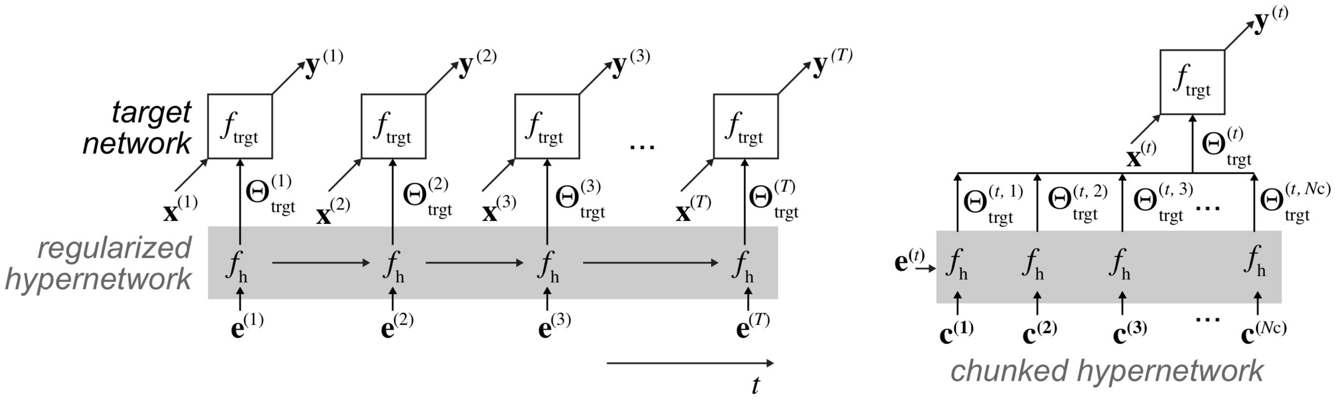
Figure 12: A diagram taken from the paper by von Oswald et al. (2019) presenting the design of the proposed approach. The full solution shown on the left, and the chunked on the right.

When evaluating the model the authors consider the same three continual learning scenarios presented in the paper by van de Ven & Tolias (2019). Two datasets are used to do this, MNIST and CIFAR-10/100. A common MNIST benchmark in continual learning is the permuted MNIST, whereby the model is first trained on the MNIST digits and subsequent tasks are created by applying random perturbations to the input pixels. This is designed to study the memory capacity of a continual learner and most appropriately fits the first continual learning scenario. The second benchmark using MNIST is the split MNIST benchmark which introduces class overlap, here the digits are sequentially paired to form five binary classification tasks. This test fits the second and third continual learning scenarios, where the model is not told which task it is performing. Finally the model is evaluated on the most challenging continual learning problem, the split CIFAR-10/100 task, where the model first learns the CIFAR-10 dataset and is then presented with sets of ten classes from the CIFAR-100 dataset, which it is asked to learn in a sequential manner. The model produced state-of-the-art results on all of these continual learning benchmarks.

It is clear such continual learning scenarios could be pertinent in the graceful degradation problem, where the system evolves with its environment. However, such approaches would require the annotation of new data in these environments. Perhaps the coalescence of active and continual learning could optimally inform which data should be annotated as this occurs. In the graceful degradation scenario this can account for unknown unknowns, provided there is intervention from the operator, as in the continual learning scenario new tasks and classes can be introduced as the learning continues. Hence, such models could be incorporated into scenarios where epistemic uncertainties are expected, if there are resources available to facilitate the learning in the system.

Sometimes such learning will be too slow to undertake after the deployment of a system and such environmental changes can be anticipated. In this scenario it may be beneficial to have a system in place that allows the quick adaptation of a system when its environment changes. This is where techniques such as domain adaptation and meta-learning could play an important role in a gracefully degrading system. Hence, these will be discussed in the next sections.

3.2 Domain Adaptation

In domain adaptation (DA) the goal is to create a system that is trained on one distribution, but operates in the context of another distribution. There exist two types of DA at the broadest level: Single-step and multi-step. In single step domain adaptation the model switches domain through a single continuous adaptation. In multi-step domain adaptation the model switches domains via an intermediate domain, once finding an appropriate intermediate domain it is easy to see the method becomes a single-step problem. Once in the single-step domain, the methods can be split again into homogenous and heterogenous. The most notable difference between these are the feature spaces in the training and target distributions. In the homogenous regime the feature spaces are the same and in heterogenous the feature spaces differ, arguably making it more akin to transfer learning. In homogenous domain adaptation the only difference is in the distributions of the sets of data, as the source and target domain share a relationship between one another. Hence, this is closely related to the graceful degradation problem, as like in the second vignette domain adaptation is about the model understanding data is outside of its training domain and re-training for the new domain. This might be a change in environment for a disaster response drone, or change of season in a smart city system.

Homogenous domain adaptation can again be split into: Discrepancy-based approaches (Balaji et al. (2019), Chen et al. (2020a), Zellinger et al. (2019), Li et al. (2020)), adversarial-based (Long et al. (2018), Cui et al. (2020b), Wang et al. (2020), Jiang et al. (2020), Tang & Jia (2020), Jiang et al. (2020)), and reconstruction-based (Gong et al. (2019), Bousmalis et al. (2016), Tang et al. (2020)). In discrepancy-based approaches the deep network is fine-tuned to diminish a discrepancy caused by the domain shift. This discrepancy can be based on a variety of criteria, such as class labels, statistical distributions, model architecture, and geometric signatures. In adversarial-based approaches domain discriminators encourage domain confusion through an adversarial objective, this might use generative or non-generative approaches. Reconstruction-based approaches use data reconstruction as an auxiliary task ensuring feature invariance. Of course, there are some approaches that do not fit into this segregation, such as the heuristic approach shown in the paper by Cui et al. (2020a) and a semi-supervised approach presented by Zhang et al. (2020). It is also worth noting these approaches share some resemblance to transfer learning and many techniques will be seen in both fields, the main difference being in domain adaptation there often do not exist labelled examples in the target domain.

Many of these approaches assume there exists labelled examples in the new domain, indeed all of the approaches outlined above can be undertaken in a supervised, semi-supervised, or unsupervised manner. Clearly having labelled examples in the source domain is a luxury in this problem and having unlabelled samples will be more common, hence recent papers utilising unlabelled data will be highlighted in this section.

Sun et al. (2019) present an unsupervised method of domain adaptation that utilises self-supervised learning to enable transfer between domains. Presented, is a model that learns supervised representations for a classification task, whilst performing a self-supervised task on both the source and target domain. The main contribution of the paper is presenting self-supervision tasks that are suitable for domain adaptation. Three tasks are identified: Rotation prediction, flip prediction, and patch localisation. In rotation prediction the model is trained to recognise to what angle an image has been rotated. In flip prediction whether the image has been flipped or not. Finally, in patch localisation the model is trained to return the correct coordinates on a 2x2 square for each of four quadrants of a segmented image. They also argue that multiple self-supervised tasks will help merge the target and source domains more effectively, this is demonstrated graphically in a figure from the paper shown in figure 13.

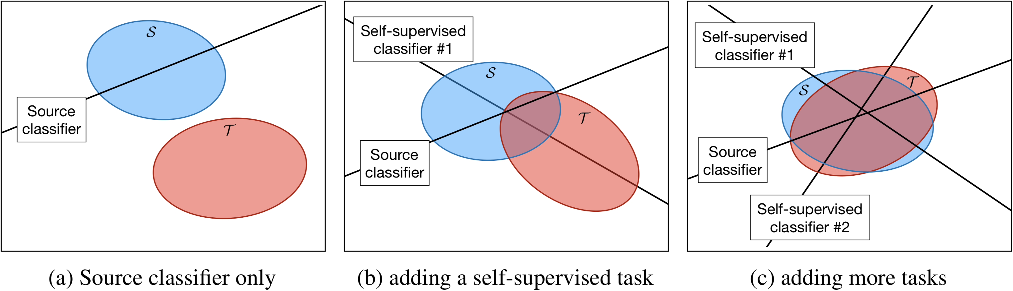
Figure 13: A figure from a paper by Sun et al. (2019) demonstrating how self-supervision tasks help align domains in the representation space.

To train the system, $K$ self supervised tasks were selected creating $K+1$ loss functions including the supervised prediction task on seen data. This creates $K+1$ classification heads ($h_{0,1...k-1,k}$) and a common feature extractor, the parameters of which are learned by the system. In this case the feature extractor is a deep CNN and the classification heads are simple linear layers. At test time all heads except $h_{0}$ are discarded, as $h_{0}$ is the classification head.

The model was tested on seven object recognition benchmarks, on four of which state-of-the-art accuracies was achieved when utilising all three self-supervision techniques. They also test their method on object segmentation but find the self-supervised tasks are designed for object detection, thus the method is not as effective. However, the paper presents state-of-the-art domain adaptation when there exists no labels in the target domain, but there is unlabelled data. It is also suggested that this technique may be effective where the amount of data in the target domain is small.

Another unsupervised method that performs better on image segmentation is presented by Biasetton et al. (2019). In the paper the authors propose a three component strategy, which uses supervised, adversarial, and a self-learning strategy. The supervised component of the model uses a synthetic dataset, GTA5 (Richter et al. (2016)) and for each scene produces a class probability label in a pixel wise manner, which is trained using a cross-entropy loss function. The second part of the model is a discriminator which aims to distinguish between generated segmentations and the ground truth segmentations, this is again done in a pixel-wise manner. Since segmentations can also be generated for the target domain, this methodology utilises target domain information in an unsupervised way, as the ground truth information is only available for the synthetic dataset. The output of the discriminator is used to create a confidence map of the segmentation, allowing a self-training procedure which ensures the predictions are deemed more reliable when the discriminator marks generated samples as ground truth more frequently. The structure of their approach is shown graphically in figure 14.

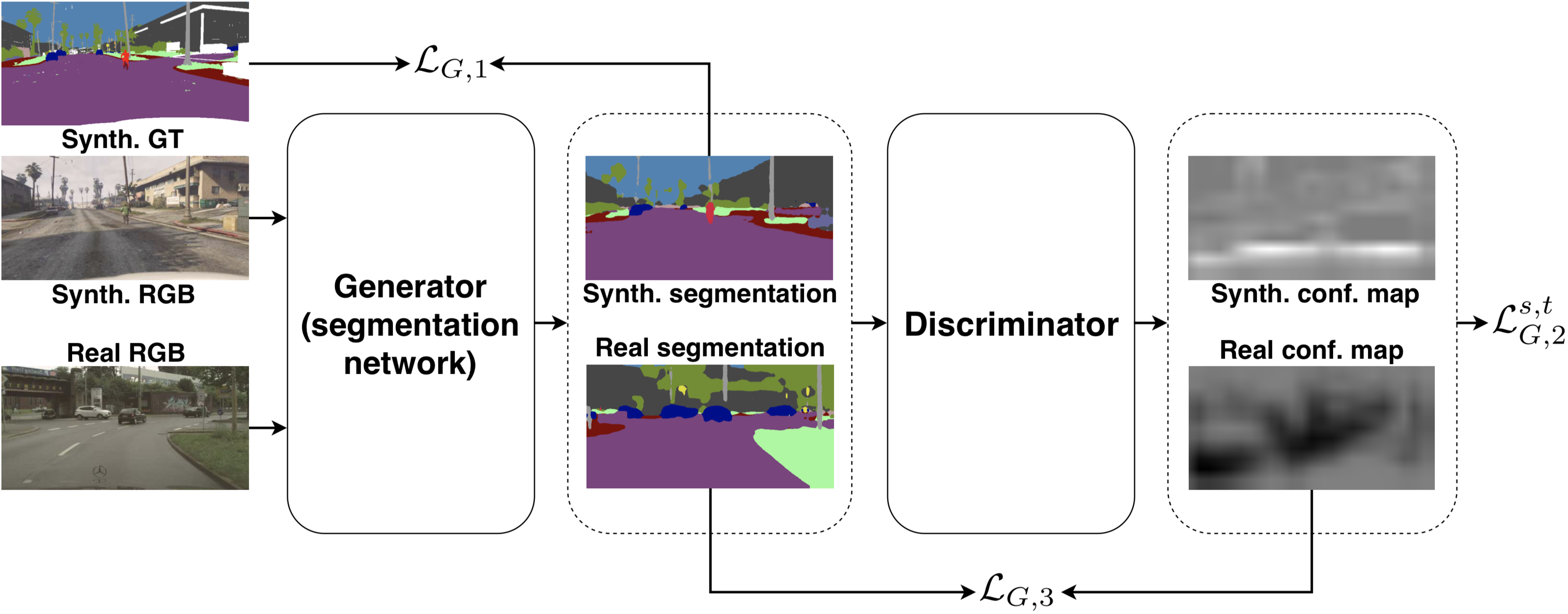
Figure 14: A figure from a paper by Biasetton et al. (2019) demonstrating how the approach is structured.

Two models were trained, one on the GTA5 dataset and one on SYNTHIA (Ros et al. (2016)), both are synthetic datasets. The model was then evaluated on the Cityscapes dataset (Cordts et al. (2016)). On average, performance on both datasets was comparable to or exceeded that of competing approaches, if falling short on a few classes.

Domain adaptation generally requires the existence of known unknowns, but is effective in overcoming the difficulty of passing between domains when the target domain lacks labelled data. Hence, the graceful degradation problem of moving outside of the training domain could be solved by using domain adaptation strategies on target domain information. Like in the examples above this is particularly useful when there are sufficient unlabelled instances of out-of-distribution data, that share the same feature space as the training data. It is clear these approaches would be used in the case of aleatoric predictive uncertainties. Such methods can be intensive during the training phase and will require large amounts of computational resources. Hence, whilst producing robustly trained networks quick adaptation might not be achievable in this paradigm. This is something meta-learning can facilitate.

3.3 Meta-Learning

Meta-learning is often referred to as the process of learning to learn, this is because the models are often trained and tested on a number of tasks and datasets. Here, the key evaluative measure is the performance of a single model across a range of tasks. A recent survey paper by Hospedales et al. (2020) proposes splitting the field across three axes that segregate approaches based on their meta-representations, meta-optimisers, and meta-objectives. These can be likened to what they learn, how they learn, and why they learn, respectively. A taxonomy taken from the paper, as well as various applications of meta-learning, is shown in figure 15.

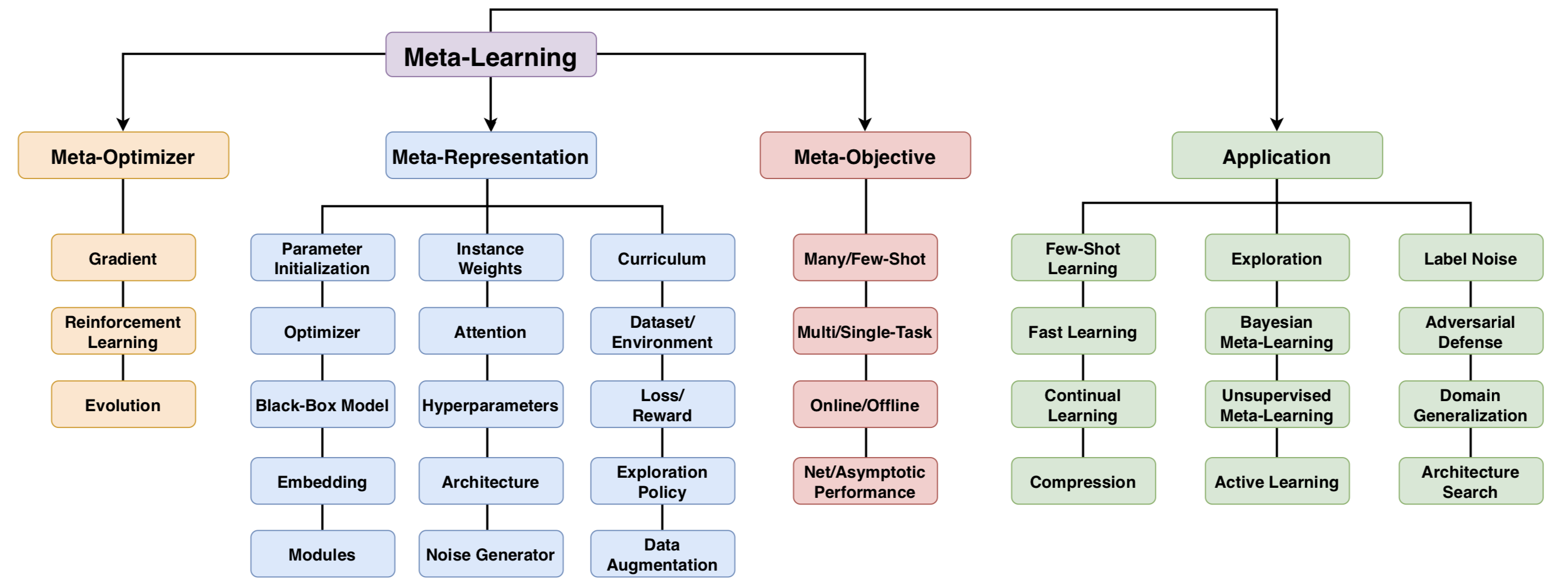
Figure 15: A figure from a survey paper by Hospedales et al. (2020) demonstrating a taxonomy of approaches in meta-learning.

Perhaps the most relevant parts of this diagram in the graceful degradation problem are the meta-representation and application parts, that is how they are implemented and where they are used. Some stand out applications for the graceful degradation include fast, continual, active, and few-shot learning, domain generalisation, and adversarial defence. Most of these applications have been discussed in this survey, suggesting meta-learning is a problem that is at the heart of adapting models in the graceful degradation environment.

Meta learning in the graceful degradation problem is most applicable to the quick adaptation of models upon encountering data outside of their training distribution, this might be fast video segmentation of new object as in Thulasidasan et al. (2019). But, if for example a change of environment or feature space is expected, the operator may have sets of training data available to quickly retrain the model. This would be the few-shot learning environment. To that end, the state-of-the-art in this area will be discussed. This area of the field can generally be split into two approaches: Gradient-based, and memory-based.

Memory based approaches utilise the memory of a recurrent neural network (RNN) to directly parameterise an update rule for the few shot problem (Andrychowicz et al. (2016), Li & Malik (2016), Chen et al. (2017), Ravi & Larochelle (2016)). Theoretically, RNNs are universal function approximators, hence should be able to represent any learning rule. In gradient based approaches the goal is to find an initialisation that can be adapted for a number of tasks through gradient descent. Papers by Finn et al. (2017) and Flennerhag et al. (2019) provided strong frameworks for this approach and have since been expanded upon in many papers (Antoniou et al. (2019), Behl et al. (2019), Yao et al. (2019), Rajeswaran et al. (2019)) and prompted unsupervised approaches as shown in a paper by Hsu et al. (2019). Recent work such as that by Lee & Choi (2018) has emphasised the use of preconditioning to more directly control the gradient descent process, merging the two approaches in the field.

Memory based approaches lack a strong inductive bias on which to base an update rule, making them hard to train. While gradient-based methods seek to find a strong inductive bias on which to make updates, but restrict knowledge transfer to the initialisation of the model. Hence, there is motivation to unify both approaches in the field, a recent example of such a unification is presented in a paper by Flennerhag et al. (2020).

The paper presents a method that updates the initialisation of the model as well as the way in which it makes gradient updates, through preconditioning. Here, preconditioning is parameterised by defining a subspace with layers in the network being dedicated to warping the activation space. This parameterises the update behaviour whilst also allowing an optimised initialisation to be found in the model. A representation of preconditioning is shown in figure 16, here the standard loss space, $\mathcal{W}$, is transformed to a simpler space, $\mathcal{P}$, for which it is easier to locate the minimum via gradient descent. This is demonstrated by the black and magenta update paths, the magenta path being the one informed by the warp layers. This is shown for two different tasks, $\mathcal{T}$ and $\mathcal{T}^{\prime}$.

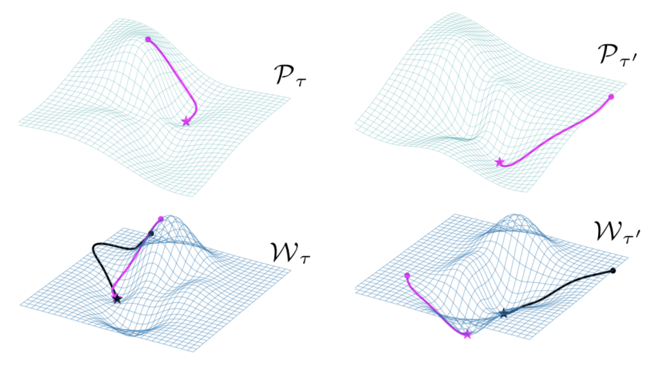
Figure 16: A figure from the paper by Flennerhag et al. (2020) comparing the loss landscapes of warped and non-warped representations.

The approach is evaluated using the popular Omniglot dataset, which is a dataset containing a variety of alphabets for character recognition (Lake et al. (2015)). To meta-train, the model is trained on one of these alphabets and tested on an unseen subset of the same alphabet. The testing losses are then backpropagated to the initialisation of the model, which includes the gradient guiding warp layers. The effectiveness of the model is evaluated on a separate set of alphabets reserved for evaluation and never meta-trained on. This avoids fitting to the evaluation tasks. The evaluation procedure is performed in the same manner as training: The meta-learnt model is trained on an alphabet and then tested on a subset of the same alphabet. The difference being the model does not see the alphabet until the evaluation stage. The approach was also evaluated on a number of other datasets including mini and tiered-ImageNet (Ren et al. (2018)), in which the method is evaluated on its ability to scale beyond few-shot classification. The work outperformed all existing approaches on all benchmarks.

Meta-learning is a field that is placed at the heart of the active approaches to the graceful degradation problem. In this setting it can be likened to the heterogenous setting of domain adaptation, where the task is changing as opposed to the domain. Whilst the paper discussed is one that uses meta-learning for few shot classification, it is clear from figure 15 that the uses of meta-learning approaches extend far beyond this, be it in domain generalisation, or active learning. However, meta-learning models can be very resource intensive to instantiate, due to the necessity to train on large amounts of data. Unsupervised meta-learning can alleviate the necessity for labelled data, but cannot remove the requirement for large amounts of data. Hence, while these methods are effective in creating effective and adaptive models, they require known unknowns and large amounts of data, limiting the use cases for such approaches. The same can be said for active and passive approaches to the problem in general, understanding when one is more applicable than the other and the constraints that can govern these decisions are important considerations to be made. To this end, applications of the approaches in this survey will be discussed in the next section.

4 Comparison and Application of Discussed Approaches

The previous sections briefly discuss the state-of-the-art in the various areas of the graceful degradation problem, discussing some interesting papers in more detail. Here, the application of such approaches will be discussed and where particular constraints might prompt the use of certain techniques. First, passive and active approaches will be compared and contrasted.

The most important factor in both passive and active approaches is uncertainty, that is, both sides of the graceful degradation problem are concerned with how they deal with uncertainty. Therefore, obtaining accurate uncertainties, both in the aleatoric and epistemic case, will be important. Where they differ is how they then manage that uncertainty. Passive approaches handle the uncertainty in a self-contained manner, naturally this limits the domains in which they can be used. This means once they are deployed updates cannot be made without to them without recalling the system. In contrast, active approaches seek to benefit from additional information and are updated according to changes in the environment or task. However, this would introduce additional difficulties when following verification and validation protocols on deployed software.

This means passive approaches will likely require less maintenance once deployed, but full functionality will likely be lost once leaving the distribution. As discussed, this can be alleviated in some way through using zero-shot learning techniques to give the model knowledge outside of the trained distribution. Furthermore, hierarchical classification models present a middle ground by offering a coarser-grained classification. However, full functionality will still be lost regardless of how epistemic uncertainty is handled. Active approaches on the other hand, whilst needing updates to ensure they are trained in the operating domains, will not lose functionality when changing environments or tasks. This means they will require ongoing maintenance as they operate across environments, but will be more adaptable than passive systems. These updates can happen at a range of magnitudes be it with individual data points, or new tasks.

A benefit to uncertainty communicating systems and to a lesser extent, hierarchical classification systems, is that they will often be effective on unknown unknowns. This means they do not require additional information to employ their functionality on out-of-distribution data. However, in active approaches changing tasks or domains will always occur with known unknowns. Hence, these methods will be undermined by uncertainties arising due to unknown unknowns, as there is no way for the model to adapt them. Small adaptations like in active and continual learning have the potential to adapt to unknown unknowns, provided the operator is able to label the unknown datapoint correctly.

A variety of supervision strategies are used across the breadth of the graceful degradation problem, with particular branches of the problem seeing more usage of one type than others. For example in domain adaptation and zero-shot models, unsupervised learning is used more often than fully supervised. As the existence of labelled data in the target environment will often negate the need for the approach in the first place. In contrast out-of-distribution detection models in uncertainty based methods will often use supervised approaches, as knowledge of out-of-distribution data will cause data leakage thus undermining the efficacy of the method. Hence, when considering the most appropriate supervision strategy the use case should be considered as well as the data that is available, as some approaches are better suited to certain supervision strategies.

Each method has benefits over the other, passive approaches will be better suited when access to the system is limited and the environment in which it operates is not likely to change. Active approaches will be better suited in scenarios where the system is likely to encounter a number of environments, which might be known to an operator beforehand. Ultimately, the usage of passive and active approaches will be determined by the computational resources available to a system, the data available to train it, and its use case. To that end, some likely scenarios and limiting cases will be considered for the remainder of the section.

Unknown unknowns

When function on unknown unknowns is needed, this will limit some of the gracefully degrading implementations available. Passive approaches that express uncertainty and obtain accurate estimations of them will be useful, some hierarchical classification systems might be available too, provided the target object is not too far out-of-distribution. In terms of active approaches both meta-learning and domain adaptation require preparation for the target distributions, hence limiting the uses to problems with known unknowns. Active and continual learning on the other hand could be used on unknown unknowns, provided the operator is able to label the unknown object. For example, in stream-based active learning the system is faced with new data continuously, some of this it will be able to classify, but some may need labelling by the operator. The same could be said for continual/lifelong learning. Therefore, the approaches that could be used when you anticipate unknown unknowns are: Active learning, continual learning, hierarchical classification, and out-of-distribution detection/accurate epistemic uncertainty models.

Low data in the target domain

When there exists a small amount of data in the target domain some approaches might be ruled out. For example some uncertainty based methods will lose functionality if they cannot be sufficiently trained in the new domain and simply return uncertainty. Zero-shot and hierarchical classification methods might be useful, but it would be more appropriate to use methods that more efficiently use the labelled data. Therefore, active approaches might be preferred in this case. For example, meta-learning could be used in the few-shot environment to quickly adapt a model to classify objects in the target domain. Domain adaptation models could be used, but the small amounts of data would likely prevent them from achieving the desired performance in the target domain, the same might be said for active and continual learning. However, if the change between domains is small active approaches may be useful as they can build upon existing representations of the data space. Therefore, when limited in the amount of data in the target domain, active approaches will likely be preferred over passive, namely active learning and meta-learning. It is also important to consider the existing knowledge of the system when selecting between these approaches.

Data is not in the target domain

In this scenario the desired functionality of the model should be considered. For example, if the aim is to classify objects in the new target domain, then zero-shot classification will be preferred as it will provide the model with a baseline understanding of the new area. If the aim is to express uncertainty when encountering the new domain, uncertainty communicating models may still be useful. Furthermore, hierarchical classification models could be useful in this scenario, providing coarse level labels on data in the new domain. However, active approaches would be rendered ineffective until data could be collected in the new domain, even then, this data would be unlabelled and will require annotation by an operator. Therefore, the most appropriate methods when there is no data in the target domain are: Zero-shot classification, hierarchical classification, and out-of-distribution detection/accurate epistemic uncertainty models.

There only exists unlabelled data

In the scenario that there is only unlabelled data in the new domain active approaches will be more useful than passive approaches. For example, domain adaptation could efficiently leverage the new data, provided the labels are the same across both domains. Meta-learning also has unsupervised methodologies, hence these could also be used to adapt the model. If an operator is available to annotate a selection of data, pool-based active learning could be implemented. Some uncertainty aware approaches that use unlabelled data could be employed. For example, unsupervised out-of-distribution techniques could be used so the system is aware that it has left the intended distribution. But such functionalities can be achieved without leveraging additional data. Hence, to make the most use of the data available an active approach would likely be preferred. But, the most appropriate active approach will be determined by the particular scenario and the availability of resources.

5 Open Challenges and Conclusion

Throughout this survey the literature of various fields related to graceful degradation have been discussed. It has shown that graceful degradation can be built into cutting edge AI enabled systems, by implementing some of the techniques discussed. However, that is not to say these fields are all optimally suited for graceful degradation. Hence, there are various open areas in which further development could be made to better enable gracefully degrading machine learning systems. In this section a number of these will be identified and conclusions of the survey will be presented.

Bayesian inference methods are very successful in giving suitable predictive uncertainty with its predictions, however they have high inference costs relative to fully deterministic models. Dynamic inference methods have shown to have impressive results in making complex models more efficient (Huang et al. (2017), Wang et al. (2017), Teerapittayanon et al. (2016), Wang et al. (2020)). Unlike other power saving methods, dynamic inference allows the full model to be used when necessary, meaning predictive uncertainty could be preserved. Efficiency at the inference stage of bayesian models is something that has not seen a lot of development, dynamic inference strategies could provide this.

In hierarchical classification hyperbolic embedding spaces have recently been implemented to better represent the hierarchy of classes. Such embedding spaces could be implemented in other models where the preservation of distances are important in the embedding space. Furthermore, as shown in a paper by Passalis et al. (2020), work has recently been done with branched neural networks to facilitate hierarchically minded representations.

Branched neural networks are an implicit and powerful form of dynamic inference that allow predictions of improving predictive uncertainty at the expense of increasing computational expense. This allows for an input adaptive system that can quickly and confidently classify easy samples, but will use more computational resources on hard samples. Hierarchical bayesian inference would compliment such models, allowing for confident and efficient inference at varying levels of class hierarchy, or alternatively, fast confident bayesian inference utilising early exiting strategies.

As discussed, uncertainty is the core property of a gracefully degrading system, many of the methods in this survey fail to include uncertainty measures in their analysis. For example, fields such as zero-shot learning, meta-learning, and domain adaptation concentrate predominantly on the accuracy of predictions, as opposed to appropriate predictive confidence. Whilst accuracy is an important metric for such areas, the confidence of incorrect predictions should also be considered and should be minimised where possible. Hence, the uncertainty aware methods discussed in section 2.1 should be transferred to other areas if they are to be moved to the deployable domains.

There exist a lot of similarities between domain adaptation and GZSL, as the main goal is for the system to work on seen and unseen classes. The only difference between the two settings is that domain adaptation gets access to unlabelled examples of the classes. There does exist a field in the zero-shot learning field, transductive zero-shot learning, where the model has access to unlabelled examples of the unseen classes. It follows that this field is identical to domain adaptation, therefore, there is opportunity for the two areas to take inspiration from one another.

Stream-based sampling his perhaps the most relevant active learning approach as it most appropriately reflects the operator–system scenario, whereby the system will consult an oracle when it lacks confidence. However, this area is not particularly active, being replaced by pool-based sampling. If graceful degradation is to progress further, active learning approaches should be evaluated in both the pool-based and stream-based sampling settings. Hence, some future work would be a comprehensive evaluation of all state-of-the-art active learning algorithms, across both settings, to understand which techniques are the most applicable to given scenarios.

This survey began by understanding what is meant by graceful degradation and formally defined the graceful degradation problem in machine learning. It was defined as the notion of minimising the effects of out-of-distribution errors. These effects often take the form of increased errors and more importantly, over-confidence in these erroneous predictions. Following this some vignettes were considered to better understand the applications of gracefully degrading vision systems and where they might be useful.

The various approaches to the graceful degradation problem were then arranged into a taxonomy to better understand the various approaches in the field and how they can be arranged. It was understood that appropriate uncertainty is a core idea of the graceful degradation problem. Hence, uncertainty was explored as well as various uncertainty and confidence metrics. A novel fundamental split was identified in the approaches Passive and active. This allowed the graceful degradation problem to be analysed in an application-centric manner.

Using the taxonomy a comprehensive review of the field was undertaken, first starting with the passive approaches, including methods of obtaining accurate uncertainties, zero-shot classification, and hierarchical classification models. Then active approaches were considered, including active and continual learning, meta-learning, and domain adaptation. Finally some future areas of research were considered, namely suggesting that branched neural networks could interact with the graceful degradation problem in an effective manner.

This paper has formalised the graceful degradation problem and surveyed the relevant areas of the machine learning landscape. If machine learning is ever to be deployed in safety critical systems it is clear that the inclusion of graceful degradation in the design methodology is imperative. This survey has aimed to communicate the importance of the problem and prompt the development of machine learning strategies that are aware of graceful degradation.

6 Acknowledgements

This work was supported in part by the following:

• My supervisors Professor Steve Gunn and Dr Sebastian Stein for providing helpful discussions on a weekly basis

• The Alan Turing Institute for providing feedback on the development of the survey on a regular basis

• The Defence Science and Technology Laboratory for supporting the project and providing feedback on the report

• The EPSRC Centre for Doctoral Training in Machine Intelligence for Nano-electronic Devices and Systems, funded by the UK Engineering and Physical Sciences Research Council and the University of Southampton

Appendix A Github Repositories

Here, some of the papers with accompanying GitHub repositories are detailed with accompanying repositories.

A.1 Passive Approaches

A.1.1 Accurate Epistemic Uncertainties

Data/Training-Based:

Uncertainty-aware deep classifiers using generative models:

https://muratsensoy.github.io/gen.html

Improving confidence estimates on unfamiliar examples:

https://github.com/lizhitwo/ConfidenceEstimates

Model-Based:

Implicit weight uncertainty in neural networks

https://github.com/pawni/BayesByHypernet/

Weight uncertainty in neural networks:

https://github.com/saxena-mayur/Weight-Uncertainty-in-Neural-Networks

Bayesian Layers:

https://github.com/google/edward2

Bias-reduced uncertainty estimation for deep neural classifiers

https://github.com/geifmany/uncertainty_ICLR

Post-Hoc:

Beyond temperature scaling- Obtaining well-calibrated multi-class probabilities with Dirichlet calibration

https://dirichletcal.github.io/

Liklihood ratios for out of distribution detection:

https://github.com/google-research/google-research/tree/master/genomics_ood

Posterior Network: Uncertainty Estimation without OOD Samples via Density-Based Pseudo-Counts

https://github.com/sharpenb/Posterior-Network

A.1.2 Zero-shot Classification

Creativity inspired zero-shot learning

https://github.com/mhelhoseiny/CIZSL

Hyperbolic Visual Embedding Learning for Zero-Shot Recognition:

https://github.com/ShaoTengLiu/Hyperbolic_ZSL

A.2 Hierarchical Classification

A Fully Hyperbolic Neural Model for Hierarchical Multi-Class Classification

https://github.com/nlpAThits/hyfi

Hyperbolic graph convolutional neural networks:

https://github.com/facebookresearch/hgnn

Making Better Mistakes- Leveraging Class Hierarchies with Deep Networks:

https://github.com/fiveai/making-better-mistakes

Nested Learning for Multi-Granular Tasks

https://github.com/nestedlearning2019

A.3 Active Approaches

A.3.1 Active and Continual Learning

Continual Learning:

Meta-Consolidation for Continual Learning

https://github.com/JosephKJ/merlin

Brain-inspired replay for continual learning with artificial neural networks:

https://github.com/GMvandeVen/brain-inspired-replay

Memory Replay GANs- learning to generate images from new categories without forgetting:

https://github.com/WuChenshen/MeRGAN

Continual Learning of a Mixed Sequence of Similar and Dissimilar Tasks

https://github.com/ZixuanKe/CAT

Continual learning with hypernetworks

https://github.com/chrhenning/hypercl

Active Learning:

Bayesian Generative Active Deep Learning github

https://github.com/toantm/BGADL

Variational Adversarial Active Learning

https://github.com/sinhasam/vaal

A.4 Homogenous Domain Adaptation

Discrepancy based:

DLOW- Domain Flow for Adaptation and Generalization:

https://github.com/ETHRuiGong/DLOW

HoMM: Higher-order Moment Matching for Unsupervised Domain Adaptation

https://github.com/chenchao666/HoMM-Master

Adversarial-Based:

Classes Matter- A Fine-grained Adversarial Approach to Cross-domain Semantic Segmentation:

https://github.com/JDAI-CV/FADA

Implicit Class-Conditioned Domain Alignment for Unsupervised Domain Adaptation

https://github.com/xiangdal/implicit_alignment

Reconstruction-Based:

Gradually Vanishing Bridge for Adversarial Domain Adaptation

https://github.com/cuishuhao/GVB

Unsupervised Domain Adaptation via Structured Prediction Based Selective Pseudo-Labeling

https://github.com/hellowangqian/domain-adaptation-capls

A.5 Meta-learning for few-shot

Memory-Based:

Optimization as a Model for Few-Shot Learning

https://github.com/twitter/meta-learning-lstm

Gradient-Based:

Model-Agnostic Meta-Learning for Fast Adaptation of Deep Networks

github.com/cbfinn/maml

Meta-Learning with Warped Gradient Descent

https://github.com/flennerhag/warpgrad

Meta-Learning with Implicit Gradients

http://sites.google.com/view/imaml

Gradient-Based Meta-Learning with Learned Layerwise Metric and Subspace

https://github.com/yoonholee/MT-net

References

- Abdar et al. (2020) Moloud Abdar, Farhad Pourpanah, Sadiq Hussain, Dana Rezazadegan, Li Liu, Mohammad Ghavamzadeh, Paul Fieguth, Abbas Khosravi, U Rajendra Acharya, Vladimir Makarenkov, et al. A review of uncertainty quantification in deep learning: Techniques, applications and challenges. arXiv preprint arXiv:2011.06225, 2020.
- Achddou et al. (2020) Raphaël Achddou, J. Matias di Martino, and Guillermo Sapiro. Nested learning for multi-granular tasks, arXiv ID: 2007:06402, 2020.
- Ai & Kwon (2020) Sophy Ai and Jangwoo Kwon. Extreme low-light image enhancement for surveillance cameras using attention u-net. Sensors, 20(2):495, 2020.
- Aljundi et al. (2020) Rahaf Aljundi, Nikolay Chumerin, and Daniel Olmeda Reino. Identifying wrongly predicted samples: A method for active learning, arXiv preprint arXiv:2010.06890, 2020.
- Andrychowicz et al. (2016) Marcin Andrychowicz, Misha Denil, Sergio Gomez, Matthew W Hoffman, David Pfau, Tom Schaul, Brendan Shillingford, and Nando De Freitas. Learning to learn by gradient descent by gradient descent. Advances in neural information processing systems, 29:3981–3989, 2016.
- Antoniou et al. (2019) Antreas Antoniou, Harrison Edwards, and Amos Storkey. How to train your MAML. In International Conference on Learning Representations (Poster Presentation), 2019.
- Ash et al. (2019) Jordan T Ash, Chicheng Zhang, Akshay Krishnamurthy, John Langford, and Alekh Agarwal. Deep batch active learning by diverse, uncertain gradient lower bounds. In International Conference on Learning Representations (Talk), 2019.
- Balaji et al. (2019) Yogesh Balaji, Rama Chellappa, and Soheil Feizi. Normalized wasserstein for mixture distributions with applications in adversarial learning and domain adaptation. In Proceedings of the IEEE International Conference on Computer Vision, pp. 6500–6508, 2019.
- Behl et al. (2019) Harkirat Singh Behl, Atılım Güneş Baydin, and Philip HS Torr. Alpha maml: Adaptive model-agnostic meta-learning. arXiv preprint arXiv:1905.07435, 2019.
- Beluch et al. (2018) William H Beluch, Tim Genewein, Andreas Nürnberger, and Jan M Köhler. The power of ensembles for active learning in image classification. In Proceedings of the IEEE Conference on Computer Vision and Pattern Recognition, pp. 9368–9377, 2018.
- Bertinetto et al. (2020) Luca Bertinetto, Romain Mueller, Konstantinos Tertikas, Sina Samangooei, and Nicholas A. Lord. Making better mistakes: Leveraging class hierarchies with deep networks. In Proceedings of the IEEE/CVF Conference on Computer Vision and Pattern Recognition (CVPR), pp. 12506–12515, June 2020.
- Biasetton et al. (2019) Matteo Biasetton, Umberto Michieli, Gianluca Agresti, and Pietro Zanuttigh. Unsupervised domain adaptation for semantic segmentation of urban scenes. In Proceedings of the IEEE/CVF Conference on Computer Vision and Pattern Recognition (CVPR) Workshops, June 2019.
- Blundell et al. (2015) Charles Blundell, Julien Cornebise, Koray Kavukcuoglu, and Daan Wierstra. Weight uncertainty in neural networks. In Proceedings of the 32nd International Conference on International Conference on Machine Learning-Volume 37, pp. 1613–1622, 2015.
- Bousmalis et al. (2016) Konstantinos Bousmalis, George Trigeorgis, Nathan Silberman, Dilip Krishnan, and Dumitru Erhan. Domain separation networks. In Proceedings of the 30th International Conference on Neural Information Processing Systems, pp. 343–351, 2016.
- Brier (1950) Glenn W Brier. Verification of forecasts expressed in terms of probability. Monthly weather review, 78(1):1–3, 1950.
- Bucher et al. (2019) Maxime Bucher, Tuan-Hung VU, Matthieu Cord, and Patrick Pérez. Zero-shot semantic segmentation. In H. Wallach, H. Larochelle, A. Beygelzimer, F. d'Alché-Buc, E. Fox, and R. Garnett (eds.), Advances in Neural Information Processing Systems 32, pp. 468–479. Curran Associates, Inc., 2019.
- Caccia et al. (2020) Massimo Caccia, Pau Rodriguez, Oleksiy Ostapenko, Fabrice Normandin, Min Lin, Lucas Caccia, Issam Laradji, Irina Rish, Alexandre Lacoste, David Vazquez, and Laurent Charlin. Online fast adaptation and knowledge accumulation: a new approach to continual learning, arXiv: 2003.05856, 2020.
- Cha et al. (2020) Jaehoon Cha, Kyeong Soo Kim, and Sanghyuk Lee. Hierarchical auxiliary learning. Machine Learning: Science and Technology, 1(4):045002, 2020.
- Chami et al. (2019) Ines Chami, Zhitao Ying, Christopher Ré, and Jure Leskovec. Hyperbolic graph convolutional neural networks. In H. Wallach, H. Larochelle, A. Beygelzimer, F. d Alché-Buc, E. Fox, and R. Garnett (eds.), Advances in Neural Information Processing Systems, volume 32, pp. 4868–4879. Curran Associates, Inc., 2019.
- Charpentier et al. (2020) Bertrand Charpentier, Daniel Zügner, and Stephan Günnemann. Posterior network: Uncertainty estimation without ood samples via density-based pseudo-counts, arXiv: 2006.09239, 2020.
- Chen et al. (2020a) Chao Chen, Zhihang Fu, Zhihong Chen, Sheng Jin, Zhaowei Cheng, Xinyu Jin, and Xian-Sheng Hua. Homm: Higher-order moment matching for unsupervised domain adaptation. In Proceedings of the AAAI Conference on Artificial Intelligence, volume 34, pp. 3422–3429, 2020a.
- Chen et al. (2018) Tianshui Chen, Wenxi Wu, Yuefang Gao, Le Dong, Xiaonan Luo, and Liang Lin. Fine-grained representation learning and recognition by exploiting hierarchical semantic embedding. In Proceedings of the 26th ACM international conference on Multimedia, pp. 2023–2031, 2018.
- Chen et al. (2020b) Ting Chen, Simon Kornblith, Kevin Swersky, Mohammad Norouzi, and Geoffrey E Hinton. Big self-supervised models are strong semi-supervised learners. Advances in Neural Information Processing Systems (pre-proceddings), 33, 2020b.
- Chen et al. (2017) Yutian Chen, Matthew W Hoffman, Sergio Gómez Colmenarejo, Misha Denil, Timothy P Lillicrap, Matt Botvinick, and Nando Freitas. Learning to learn without gradient descent by gradient descent. In International Conference on Machine Learning, pp. 748–756. PMLR, 2017.
- Clanuwat et al. (2018) Tarin Clanuwat, Mikel Bober-Irizar, Asanobu Kitamoto, Alex Lamb, Kazuaki Yamamoto, and David Ha. Deep learning for classical japanese literature. arXiv preprint arXiv:1812.01718, 2018.
- Cong et al. (2020) Yulai Cong, Miaoyun Zhao, Jianqiao Li, Sijia Wang, and Lawrence Carin. Gan memory with no forgetting. Advances in Neural Information Processing Systems (Pre-Proceedings), 33, 2020.
- Cordts et al. (2016) Marius Cordts, Mohamed Omran, Sebastian Ramos, Timo Rehfeld, Markus Enzweiler, Rodrigo Benenson, Uwe Franke, Stefan Roth, and Bernt Schiele. The cityscapes dataset for semantic urban scene understanding. In Proceedings of the IEEE conference on computer vision and pattern recognition, pp. 3213–3223, 2016.
- Cui et al. (2020a) Shuhao Cui, Xuan Jin, Shuhui Wang, Yuan He, and Qingming Huang. Heuristic domain adaptation. In Advances in Neural Information Processing Systems (Pre-Proceedings), 2020a.
- Cui et al. (2020b) Shuhao Cui, Shuhui Wang, Junbao Zhuo, Chi Su, Qingming Huang, and Qi Tian. Gradually vanishing bridge for adversarial domain adaptation. In Proceedings of the IEEE/CVF Conference on Computer Vision and Pattern Recognition, pp. 12455–12464, 2020b.
- Deng et al. (2009) Jia Deng, Wei Dong, Richard Socher, Li-Jia Li, Kai Li, and Li Fei-Fei. Imagenet: A large-scale hierarchical image database. In 2009 IEEE conference on computer vision and pattern recognition, pp. 248–255. Ieee, 2009.
- Deng et al. (2014) Jia Deng, Nan Ding, Yangqing Jia, Andrea Frome, Kevin Murphy, Samy Bengio, Yuan Li, Hartmut Neven, and Hartwig Adam. Large-scale object classification using label relation graphs. In European conference on computer vision, pp. 48–64. Springer, 2014.
- Dhall et al. (2020) Ankit Dhall, Anastasia Makarova, Octavian Ganea, Dario Pavllo, Michael Greeff, and Andreas Krause. Hierarchical image classification using entailment cone embeddings, arXiv: 2004.03459, 2020.
- Dosovitskiy et al. (2020) Alexey Dosovitskiy, Lucas Beyer, Alexander Kolesnikov, Dirk Weissenborn, Xiaohua Zhai, Thomas Unterthiner, Mostafa Dehghani, Matthias Minderer, Georg Heigold, Sylvain Gelly, Jakob Uszkoreit, and Neil Houlsby. An image is worth 16x16 words: Transformers for image recognition at scale, arXiv: 2010.11929, 2020.
- Duan et al. (2003) Kaibo Duan, S Sathiya Keerthi, Wei Chu, Shirish Krishnaj Shevade, and Aun Neow Poo. Multi-category classification by soft-max combination of binary classifiers. In International Workshop on Multiple Classifier Systems, pp. 125–134. Springer, 2003.
- Elhoseiny & Elfeki (2019) Mohamed Elhoseiny and Mohamed Elfeki. Creativity inspired zero-shot learning. In Proceedings of the IEEE International Conference on Computer Vision, pp. 5784–5793, 2019.
- Faghri et al. (2017) Fartash Faghri, David J Fleet, Jamie Ryan Kiros, and Sanja Fidler. Vse++: Improving visual-semantic embeddings with hard negatives. arXiv preprint arXiv:1707.05612, 2017.
- Farhadi et al. (2009) Ali Farhadi, Ian Endres, Derek Hoiem, and David Forsyth. Describing objects by their attributes. In 2009 IEEE Conference on Computer Vision and Pattern Recognition, pp. 1778–1785. IEEE, 2009.
- Finn et al. (2017) Chelsea Finn, Pieter Abbeel, and Sergey Levine. Model-agnostic meta-learning for fast adaptation of deep networks. In International Conference on Machine Learning, pp. 1126–1135, 2017.
- Flennerhag et al. (2019) Sebastian Flennerhag, Pablo Garcia Moreno, Neil Lawrence, and Andreas Damianou. Transferring knowledge across learning processes. In International Conference on Learning Representations (Talk), 2019.
- Flennerhag et al. (2020) Sebastian Flennerhag, Andrei A. Rusu, Razvan Pascanu, Francesco Visin, Hujun Yin, and Raia Hadsell. Meta-learning with warped gradient descent. In International Conference on Learning Representations (Talk), 2020.
- Foret et al. (2020) Pierre Foret, Ariel Kleiner, Hossein Mobahi, and Behnam Neyshabur. Sharpness-aware minimization for efficiently improving generalization, arXiv:2010.01412, 2020.
- Fujii & Kashima (2016) Kaito Fujii and Hisashi Kashima. Budgeted stream-based active learning via adaptive submodular maximization. In Advances in Neural Information Processing Systems, pp. 514–522, 2016.
- Gal & Ghahramani (2016) Y Gal and Z Ghahramani. Dropout as a bayesian approximation: Representing model uncertainty in deep learning. In 33rd International Conference on Machine Learning, ICML 2016, volume 3, pp. 1651–1660, 2016.
- Geifman et al. (2019) Yonatan Geifman, Guy Uziel, and Ran El-Yaniv. Bias-reduced uncertainty estimation for deep neural classifiers. In International Conference on Learning Representations (Poster), 2019.
- Gong et al. (2019) Rui Gong, Wen Li, Yuhua Chen, and Luc Van Gool. Dlow: Domain flow for adaptation and generalization. In Proceedings of the IEEE Conference on Computer Vision and Pattern Recognition, pp. 2477–2486, 2019.
- Good (1952) I. J. Good. Rational decisions. Journal of the Royal Statistical Society. Series B (Methodological), 14(1):107–114, 1952. ISSN 00359246.
- Grassa et al. (2020) Riccardo La Grassa, Ignazio Gallo, and Nicola Landro. Learn class hierarchy using convolutional neural networks, arXiv: 2005.08622, 2020.
- Guo et al. (2018) Yanming Guo, Yu Liu, Erwin M Bakker, Yuanhao Guo, and Michael S Lew. Cnn-rnn: A large-scale hierarchical image classification framework. Multimedia Tools and Applications, 77(8):10251–10271, 2018.
- Ha et al. (2016) David Ha, Andrew Dai, and Quoc V. Le. Hypernetworks, arXiv: 1609.09106, 2016.
- Hafner et al. (2020) Danijar Hafner, Dustin Tran, Timothy Lillicrap, Alex Irpan, and James Davidson. Noise contrastive priors for functional uncertainty. In Uncertainty in Artificial Intelligence, pp. 905–914. PMLR, 2020.
- Han et al. (2020) Zongyan Han, Zhenyong Fu, and Jian Yang. Learning the redundancy-free features for generalized zero-shot object recognition. In Proceedings of the IEEE/CVF Conference on Computer Vision and Pattern Recognition (CVPR), pp. 12865–12874, June 2020.
- Hein et al. (2019) Matthias Hein, Maksym Andriushchenko, and Julian Bitterwolf. Why relu networks yield high-confidence predictions far away from the training data and how to mitigate the problem. In Proceedings of the IEEE/CVF Conference on Computer Vision and Pattern Recognition (CVPR), pp. 41–50, June 2019.
- Hendrycks & Gimpel (2016) Dan Hendrycks and Kevin Gimpel. A baseline for detecting misclassified and out-of-distribution examples in neural networks. arXiv preprint arXiv:1610.02136, 2016.
- Herlihy & Wing (1991) Maurice P Herlihy and Jeannette M Wing. Specifying graceful degradation. IEEE Transactions on Parallel and Distributed Systems, 2(1):93–104, 1991.
- Hong & Chae (2020) Songnam Hong and Jeongmin Chae. Active learning with multiple kernels. arXiv preprint arXiv:2005.03188, 2020.
- Hospedales et al. (2020) Timothy Hospedales, Antreas Antoniou, Paul Micaelli, and Amos Storkey. Meta-learning in neural networks: A survey, arXiv: 2004.05439, 2020.
- Hsu et al. (2019) Kyle Hsu, Sergey Levine, and Chelsea Finn. Unsupervised learning via meta-learning. In International Conference on Learning Representations (Poster), 2019.
- Hu et al. (2020) Ting-Kuei Hu, Tianlong Chen, Haotao Wang, and Zhangyang Wang. Triple wins: Boosting accuracy, robustness and efficiency together by enabling input-adaptive inference. arXiv preprint arXiv:2002.10025, 2020.
- Huang et al. (2017) Gao Huang, Danlu Chen, Tianhong Li, Felix Wu, Laurens van der Maaten, and Kilian Q Weinberger. Multi-scale dense networks for resource efficient image classification. arXiv preprint arXiv:1703.09844, 2017.
- Huynh & Elhamifar (2020) Dat Huynh and Ehsan Elhamifar. Fine-grained generalized zero-shot learning via dense attribute-based attention. In Proceedings of the IEEE/CVF Conference on Computer Vision and Pattern Recognition, pp. 4483–4493, 2020.
- Hüllermeier & Waegeman (2020) Eyke Hüllermeier and Willem Waegeman. Aleatoric and epistemic uncertainty in machine learning: An introduction to concepts and methods, arXiv: 1910.09457, 2020.
- Jiang et al. (2020) Xiang Jiang, Qicheng Lao, Stan Matwin, and Mohammad Havaei. Implicit class-conditioned domain alignment for unsupervised domain adaptation, arXiv preprint arXiv:2006.04996, 2020.
- Jospin et al. (2020) Laurent Valentin Jospin, Wray Buntine, Farid Boussaid, Ham Laga, and Mohammed Bennamoun. Hands-on bayesian neural networks-a tutorial for deep learning users. ACM Comput. Surv, 1(1), 2020.
- Jumper (2020) John Jumper. High accuracy protein structure prediction using deep learning, In Fourteenth Critical Assessment of Techniques for Protein Structure Prediction (Abstract Book), 30 November, 2020.
- Jung et al. (2020) Sangwon Jung, Hongjoon Ahn, Sungmin Cha, and Taesup Moon. Adaptive group sparse regularization for continual learning. arXiv preprint arXiv:2003.13726, 2020.
- k. Nakano et al. (2017) F. k. Nakano, S. Martiello Mastelini, S. Barbon, and R. Cerri. Stacking methods for hierarchical classification. In 2017 16th IEEE International Conference on Machine Learning and Applications (ICMLA), pp. 289–296, 2017.
- Kachman et al. (2019) Tal Kachman, Michal Moshkovitz, and Michal Rosen-Zvi. Novel uncertainty framework for deep learning ensembles, arXiv: 1904.04917, 2019.
- Kamoi & Kobayashi (2020) Ryo Kamoi and Kei Kobayashi. Why is the mahalanobis distance effective for anomaly detection?, arXiv: 2003.00402, 2020.
- Ke et al. (2020) Zixuan Ke, Bing Liu, and Xingchang Huang. Continual learning of a mixed sequence of similar and dissimilar tasks. Advances in Neural Information Processing Systems (Poster), 33, 2020.
- Keshari et al. (2020) Rohit Keshari, Richa Singh, and Mayank Vatsa. Generalized zero-shot learning via over-complete distribution. In Proceedings of the IEEE/CVF Conference on Computer Vision and Pattern Recognition, pp. 13300–13308, 2020.
- Khrulkov et al. (2020) Valentin Khrulkov, Leyla Mirvakhabova, Evgeniya Ustinova, Ivan Oseledets, and Victor Lempitsky. Hyperbolic image embeddings. In Proceedings of the IEEE/CVF Conference on Computer Vision and Pattern Recognition (CVPR), pp. 6418–6428, June 2020.
- Kihara et al. (2019) Tomo Kihara, Roy Bendor, and Derek Lomas. Designing an escape room in the city for public engagement with ai-enhanced surveillance. In Extended Abstracts of the 2019 CHI Conference on Human Factors in Computing Systems, pp. 1–6, 2019.
- Kingma & Welling (2013) Diederik P Kingma and Max Welling. Auto-encoding variational bayes. arXiv preprint arXiv:1312.6114, 2013.
- KJ & Nallure Balasubramanian (2020) Joseph KJ and Vineeth Nallure Balasubramanian. Meta-consolidation for continual learning. Advances in Neural Information Processing Systems (Pre-Proceedings), 33, 2020.
- Koo et al. (2019) Jaehoon Koo, Diego Klabjan, and Jean Utke. Combined convolutional and recurrent neural networks for hierarchical classification of images, arXiv: 1809.09574, 2019.
- Kull et al. (2019) Meelis Kull, Miquel Perello Nieto, Markus Kängsepp, Telmo Silva Filho, Hao Song, and Peter Flach. Beyond temperature scaling: Obtaining well-calibrated multi-class probabilities with dirichlet calibration. Advances in neural information processing systems, 32:12316–12326, 2019.
- Kumar & Zheng (2017) Suren Kumar and Rui Zheng. Hierarchical category detector for clothing recognition from visual data. In Proceedings of the IEEE International Conference on Computer Vision Workshops, pp. 2306–2312, 2017.
- Kurakin et al. (2017) Alexey Kurakin, Ian Goodfellow, and Samy Bengio. Adversarial examples in the physical world, arXiv: 1607.02533, 2017.
- Lake et al. (2015) Brenden M Lake, Ruslan Salakhutdinov, and Joshua B Tenenbaum. Human-level concept learning through probabilistic program induction. Science, 350(6266):1332–1338, 2015.
- Lampert et al. (2013) Christoph H Lampert, Hannes Nickisch, and Stefan Harmeling. Attribute-based classification for zero-shot visual object categorization. IEEE transactions on pattern analysis and machine intelligence, 36(3):453–465, 2013.
- Lee et al. (2018a) Kimin Lee, Honglak Lee, Kibok Lee, and Jinwoo Shin. Training confidence-calibrated classifiers for detecting out-of-distribution samples, arXiv: 1711.09325, 2018a.
- Lee et al. (2018b) Kimin Lee, Kibok Lee, Honglak Lee, and Jinwoo Shin. A simple unified framework for detecting out-of-distribution samples and adversarial attacks, arXiv: 1807.03888, 2018b.
- Lee & Choi (2018) Yoonho Lee and Seungjin Choi. Gradient-based meta-learning with learned layerwise metric and subspace. In International Conference on Machine Learning, pp. 2927–2936, 2018.
- Levinthal (1969) Cyrus Levinthal. How to fold graciously. Mossbauer spectroscopy in biological systems, 67:22–24, 1969.
- Li & Malik (2016) Ke Li and Jitendra Malik. Learning to optimize, arXiv preprint arXiv:1606.01885, 2016.
- Li et al. (2020) Shuang Li, Chi Harold Liu, Qiuxia Lin, Binhui Xie, Zhengming Ding, Gao Huang, and Jian Tang. Domain conditioned adaptation network. In Thirty-Fourth AAAI Conference on Artificial Intelligence (AAAI-20), pp. 11386–11393, 2020.
- Li & Hoiem (2020) Zhizhong Li and Derek Hoiem. Improving confidence estimates for unfamiliar examples. In Proceedings of the IEEE/CVF Conference on Computer Vision and Pattern Recognition (CVPR), pp. 2686–2695, June 2020.
- Liu et al. (2020) Shaoteng Liu, Jingjing Chen, Liangming Pan, Chong-Wah Ngo, Tat-Seng Chua, and Yu-Gang Jiang. Hyperbolic visual embedding learning for zero-shot recognition. In Proceedings of the IEEE/CVF Conference on Computer Vision and Pattern Recognition, pp. 9273–9281, 2020.
- Long et al. (2018) Mingsheng Long, ZHANGJIE CAO, Jianmin Wang, and Michael I Jordan. Conditional adversarial domain adaptation. In S. Bengio, H. Wallach, H. Larochelle, K. Grauman, N. Cesa-Bianchi, and R. Garnett (eds.), Advances in Neural Information Processing Systems, volume 31, pp. 1640–1650. Curran Associates, Inc., 2018.
- López & Strube (2020) Federico López and Michael Strube. A fully hyperbolic neural model for hierarchical multi-class classification, arXiv: 2010.02053, 2020.
- Malinin & Gales (2018) Andrey Malinin and Mark Gales. Predictive uncertainty estimation via prior networks. In Advances in Neural Information Processing Systems, pp. 7047–7058, 2018.
- Mallya & Lazebnik (2018) Arun Mallya and Svetlana Lazebnik. Packnet: Adding multiple tasks to a single network by iterative pruning. In Proceedings of the IEEE Conference on Computer Vision and Pattern Recognition, pp. 7765–7773, 2018.
- Mikolov et al. (2013) Tomas Mikolov, Kai Chen, Greg Corrado, and Jeffrey Dean. Efficient estimation of word representations in vector space. arXiv preprint arXiv:1301.3781, 2013.
- Mirzadeh et al. (2020) Seyed Iman Mirzadeh, Mehrdad Farajtabar, Razvan Pascanu, and Hassan Ghasemzadeh. Understanding the role of training regimes in continual learning. Advances in Neural Information Processing Systems (Pre-Proceedings), 33, 2020.
- Murugesan & Carbonell (2017) Keerthiram Murugesan and Jaime Carbonell. Active learning from peers. In Advances in neural information processing systems, pp. 7008–7017, 2017.
- Naeini et al. (2015) Mahdi Pakdaman Naeini, Gregory F Cooper, and Milos Hauskrecht. Obtaining well calibrated probabilities using bayesian binning. In Proceedings of the… AAAI Conference on Artificial Intelligence. AAAI Conference on Artificial Intelligence, volume 2015, pp. 2901. NIH Public Access, 2015.
- Nakano et al. (2020) Felipe Kenji Nakano, Ricardo Cerri, and Celine Vens. Active learning for hierarchical multi-label classification. Data Mining and Knowledge Discovery, 34(5):1496–1530, 2020.
- Netzer et al. (2011) Yuval Netzer, Tao Wang, Adam Coates, Alessandro Bissacco, Bo Wu, and Andrew Y Ng. Reading digits in natural images with unsupervised feature learning, 2011.
- Ni et al. (2019) Jian Ni, Shanghang Zhang, and Haiyong Xie. Dual adversarial semantics-consistent network for generalized zero-shot learning. In Advances in Neural Information Processing Systems, pp. 6146–6157, 2019.
- Nickel & Kiela (2017) Maximillian Nickel and Douwe Kiela. Poincaré embeddings for learning hierarchical representations. In I. Guyon, U. V. Luxburg, S. Bengio, H. Wallach, R. Fergus, S. Vishwanathan, and R. Garnett (eds.), Advances in Neural Information Processing Systems, volume 30, pp. 6338–6347. Curran Associates, Inc., 2017.
- Norouzi et al. (2014) Mohammad Norouzi, Tomas Mikolov, Samy Bengio, Yoram Singer, Jonathon Shlens, Andrea Frome, Greg S. Corrado, and Jeffrey Dean. Zero-shot learning by convex combination of semantic embeddings, arXiv: 1312.5620, 2014.
- Oberdiek et al. (2018) Philipp Oberdiek, Matthias Rottmann, and Hanno Gottschalk. Classification uncertainty of deep neural networks based on gradient information, arXiv: 1805.08440, 2018.
- Pan et al. (2020) Pingbo Pan, Siddharth Swaroop, Alexander Immer, Runa Eschenhagen, Richard E Turner, and Mohammad Emtiyaz Khan. Continual deep learning by functional regularisation of memorable past. arXiv preprint arXiv:2004.14070, 2020.
- Passalis et al. (2020) Nikolaos Passalis, Jenni Raitoharju, Anastasios Tefas, and Moncef Gabbouj. Efficient adaptive inference for deep convolutional neural networks using hierarchical early exits. Pattern Recognition, 105:107346, 2020.
- Patterson & Hays (2012) Genevieve Patterson and James Hays. Sun attribute database: Discovering, annotating, and recognizing scene attributes. In 2012 IEEE Conference on Computer Vision and Pattern Recognition, pp. 2751–2758. IEEE, 2012.
- Pawlowski et al. (2018) Nick Pawlowski, Andrew Brock, Matthew C. H. Lee, Martin Rajchl, and Ben Glocker. Implicit weight uncertainty in neural networks, arXiv: 1711.01297, 2018.
- Pouransari & Tuzel (2020) Hadi Pouransari and Oncel Tuzel. Extracurricular learning: Knowledge transfer beyond empirical distribution, arXiv: 2007.00051, 2020.
- Radovic et al. (2017) Matija Radovic, Offei Adarkwa, and Qiaosong Wang. Object recognition in aerial images using convolutional neural networks. Journal of Imaging, 3(2):21, 2017.
- Rajeswaran et al. (2019) Aravind Rajeswaran, Chelsea Finn, Sham M Kakade, and Sergey Levine. Meta-learning with implicit gradients. In H. Wallach, H. Larochelle, A. Beygelzimer, F. d'Alché-Buc, E. Fox, and R. Garnett (eds.), Advances in Neural Information Processing Systems, volume 32, pp. 113–124. Curran Associates, Inc., 2019.
- Ramalho & Miranda (2019) Tiago Ramalho and Miguel Miranda. Density estimation in representation space to predict model uncertainty, arXiv: 1908.07235, 2019.
- Ratzlaff & Fuxin (2020) Neale Ratzlaff and Li Fuxin. Hypergan: A generative model for diverse, performant neural networks, arXiv: 1901.11058, 2020.
- Ravi & Larochelle (2016) Sachin Ravi and Hugo Larochelle. Optimization as a model for few-shot learning. International Conference on Learning Representations (Talk), 2016.
- Reed et al. (2016) Scott Reed, Zeynep Akata, Honglak Lee, and Bernt Schiele. Learning deep representations of fine-grained visual descriptions. In Proceedings of the IEEE Conference on Computer Vision and Pattern Recognition, pp. 49–58, 2016.
- Ren et al. (2019) Jie Ren, Peter J. Liu, Emily Fertig, Jasper Snoek, Ryan Poplin, Mark Depristo, Joshua Dillon, and Balaji Lakshminarayanan. Likelihood ratios for out-of-distribution detection. In H. Wallach, H. Larochelle, A. Beygelzimer, F. d Alché-Buc, E. Fox, and R. Garnett (eds.), Advances in Neural Information Processing Systems 32, pp. 14707–14718. Curran Associates, Inc., 2019.
- Ren et al. (2018) Mengye Ren, Eleni Triantafillou, Sachin Ravi, Jake Snell, Kevin Swersky, Joshua B Tenenbaum, Hugo Larochelle, and Richard S Zemel. Meta-learning for semi-supervised few-shot classification. arXiv preprint arXiv:1803.00676, 2018.
- Richter et al. (2016) Stephan R Richter, Vibhav Vineet, Stefan Roth, and Vladlen Koltun. Playing for data: Ground truth from computer games. In European conference on computer vision, pp. 102–118. Springer, 2016.
- Ros et al. (2016) German Ros, Laura Sellart, Joanna Materzynska, David Vazquez, and Antonio M Lopez. The synthia dataset: A large collection of synthetic images for semantic segmentation of urban scenes. In Proceedings of the IEEE conference on computer vision and pattern recognition, pp. 3234–3243, 2016.
- Sariyildiz & Cinbis (2019) Mert Bulent Sariyildiz and Ramazan Gokberk Cinbis. Gradient matching generative networks for zero-shot learning. In Proceedings of the IEEE Conference on Computer Vision and Pattern Recognition, pp. 2168–2178, 2019.
- Sensoy et al. (2018) Murat Sensoy, Lance Kaplan, and Melih Kandemir. Evidential deep learning to quantify classification uncertainty. In S. Bengio, H. Wallach, H. Larochelle, K. Grauman, N. Cesa-Bianchi, and R. Garnett (eds.), Advances in Neural Information Processing Systems 31, pp. 3179–3189. Curran Associates, Inc., 2018.
- Sensoy et al. (2020) Murat Sensoy, Lance Kaplan, Federico Cerutti, and Maryam Saleki. Uncertainty-aware deep classifiers using generative models, arXiv: 2006.04183, 2020.
- Seo & shik Shin (2019) Yian Seo and Kyung shik Shin. Hierarchical convolutional neural networks for fashion image classification. Expert Systems with Applications, 116:328 – 339, 2019. ISSN 0957-4174.
- Shah & Manwani (2020) Kulin Shah and Naresh Manwani. Online active learning of reject option classifiers. Proceedings of the AAAI Conference on Artificial Intelligence, 34(04):5652–5659, Apr. 2020. doi: 10.1609/aaai.v34i04.6019.
- Shao et al. (2020) Zhihui Shao, Jianyi Yang, and Shaolei Ren. Calibrating deep neural network classifiers on out-of-distribution datasets, arXiv: 2006.08914, 2020.
- Shi & Yu (2019) Weishi Shi and Qi Yu. Integrating bayesian and discriminative sparse kernel machines for multi-class active learning. In Advances in Neural Information Processing Systems, pp. 2285–2294, 2019.
- Silver et al. (2017) David Silver, Thomas Hubert, Julian Schrittwieser, Ioannis Antonoglou, Matthew Lai, Arthur Guez, Marc Lanctot, Laurent Sifre, Dharshan Kumaran, Thore Graepel, et al. Mastering chess and shogi by self-play with a general reinforcement learning algorithm. arXiv preprint arXiv:1712.01815, 2017.
- Singh et al. (2020) Pravendra Singh, Vinay Kumar Verma, Pratik Mazumder, Lawrence Carin, and Piyush Rai. Calibrating cnns for lifelong learning. Advances in Neural Information Processing Systems (Pre-Proceedings), 33, 2020.
- Sinha et al. (2019) Samarth Sinha, Sayna Ebrahimi, and Trevor Darrell. Variational adversarial active learning. In Proceedings of the IEEE International Conference on Computer Vision, pp. 5972–5981, 2019.
- Sun et al. (2019) Yu Sun, Eric Tzeng, Trevor Darrell, and Alexei A. Efros. Unsupervised domain adaptation through self-supervision, arXiv: 1909.11825, 2019.
- Tang & Jia (2020) Hui Tang and Kui Jia. Discriminative adversarial domain adaptation. In Association for the Advancement of Artificial Intelligence (AAAI), pp. 5940–5947, 2020.
- Tang et al. (2020) Hui Tang, Ke Chen, , and Kui Jia. Unsupervised domain adaptation via structurally regularized deep clustering. In IEEE Conference on Computer Vision and Pattern Recognition (CVPR), pp. 8725–8735, 2020.
- Teerapittayanon et al. (2016) Surat Teerapittayanon, Bradley McDanel, and Hsiang-Tsung Kung. Branchynet: Fast inference via early exiting from deep neural networks. In 2016 23rd International Conference on Pattern Recognition (ICPR), pp. 2464–2469. IEEE, 2016.
- Thulasidasan et al. (2019) Sunil Thulasidasan, Gopinath Chennupati, Jeff A Bilmes, Tanmoy Bhattacharya, and Sarah Michalak. On mixup training: Improved calibration and predictive uncertainty for deep neural networks. In H. Wallach, H. Larochelle, A. Beygelzimer, F. d Alché-Buc, E. Fox, and R. Garnett (eds.), Advances in Neural Information Processing Systems 32, pp. 13888–13899. Curran Associates, Inc., 2019.
- Tran et al. (2019a) Dustin Tran, Mike Dusenberry, Mark van der Wilk, and Danijar Hafner. Bayesian layers: A module for neural network uncertainty. In Advances in Neural Information Processing Systems, pp. 14660–14672, 2019a.
- Tran et al. (2019b) Toan Tran, Thanh-Toan Do, Ian Reid, and Gustavo Carneiro. Bayesian generative active deep learning. In International Conference on Machine Learning, pp. 6295–6304, 2019b.
- van de Ven & Tolias (2019) Gido M. van de Ven and Andreas S. Tolias. Three scenarios for continual learning, arXiv: 1904.07734, 2019.
- van de Ven et al. (2020) Gido M van de Ven, Hava T Siegelmann, and Andreas S Tolias. Brain-inspired replay for continual learning with artificial neural networks. Nature communications, 11(1):1–14, 2020.
- van Gemert et al. (2015) Jan C. van Gemert, Camiel R. Verschoor, Pascal Mettes, Kitso Epema, Lian Pin Koh, and Serge Wich. Nature conservation drones for automatic localization and counting of animals. In Lourdes Agapito, Michael M. Bronstein, and Carsten Rother (eds.), Computer Vision - ECCV 2014 Workshops, pp. 255–270, Cham, 2015. Springer International Publishing. ISBN 978-3-319-16178-5.
- von Oswald et al. (2019) Johannes von Oswald, Christian Henning, João Sacramento, and Benjamin F Grewe. Continual learning with hypernetworks. In International Conference on Learning Representations (Spotlight), 2019.
- Wah et al. (2011) Catherine Wah, Steve Branson, Peter Welinder, Pietro Perona, and Serge Belongie. The caltech-ucsd birds-200-2011 dataset, 2011.
- Wang et al. (2020) Haoran Wang, Tong Shen, Wei Zhang, Lingyu Duan, and Tao Mei. Classes matter: A fine-grained adversarial approach to cross-domain semantic segmentation. In The European Conference on Computer Vision (ECCV), pp. 642–659, August 2020.
- Wang et al. (2017) Xin Wang, Fisher Yu, Zi-Yi Dou, Trevor Darrell, and Joseph E. Gonzalez. Skipnet: Learning dynamic routing in convolutional networks, arXiv: 1711.09485, 2017.
- Wang et al. (2020) Y. Wang, J. Shen, T. K. Hu, P. Xu, T. Nguyen, R. Baraniuk, Z. Wang, and Y. Lin. Dual dynamic inference: Enabling more efficient, adaptive, and controllable deep inference. IEEE Journal of Selected Topics in Signal Processing, 14(4):623–633, 2020.
- Winkens et al. (2020) Jim Winkens, Rudy Bunel, Abhijit Guha Roy, Robert Stanforth, Vivek Natarajan, Joseph R. Ledsam, Patricia MacWilliams, Pushmeet Kohli, Alan Karthikesalingam, Simon Kohl, Taylan Cemgil, S. M. Ali Eslami, and Olaf Ronneberger. Contrastive training for improved out-of-distribution detection, arXiv: 2007.05566, 2020.
- Wu et al. (2020) Jiamin Wu, Tianzhu Zhang, Zheng-Jun Zha, Jiebo Luo, Yongdong Zhang, and Feng Wu. Self-supervised domain-aware generative network for generalized zero-shot learning. In Proceedings of the IEEE/CVF Conference on Computer Vision and Pattern Recognition, pp. 12767–12776, 2020.
- Yang & Loog (2018) Yazhou Yang and Marco Loog. A variance maximization criterion for active learning. Pattern Recognition, 78:358–370, 2018.
- Yao et al. (2019) Huaxiu Yao, Ying Wei, Junzhou Huang, and Zhenhui Li. Hierarchically structured meta-learning. In International Conference on Machine Learning, pp. 7045–7054, 2019.
- Yoo & Kweon (2019) Donggeun Yoo and In So Kweon. Learning loss for active learning. In Proceedings of the IEEE Conference on Computer Vision and Pattern Recognition, pp. 93–102, 2019.
- Yu & Aizawa (2019) Qing Yu and Kiyoharu Aizawa. Unsupervised out-of-distribution detection by maximum classifier discrepancy. In Proceedings of the IEEE International Conference on Computer Vision, pp. 9518–9526, 2019.
- Yu et al. (2020) Yunlong Yu, Zhong Ji, Zhongfei Zhang, and Jungong Han. Episode-based prototype generating network for zero-shot learning, arXiv: 1909.03360, 2020.
- Zellinger et al. (2019) Werner Zellinger, Bernhard A. Moser, Thomas Grubinger, Edwin Lughofer, Thomas Natschläger, and Susanne Saminger-Platz. Robust unsupervised domain adaptation for neural networks via moment alignment. Information Sciences, 483:174 – 191, 2019. ISSN 0020-0255.
- Zhang et al. (2020) Yabin Zhang, Bin Deng, Kui Jia, and Lei Zhang. Label propagation with augmented anchors: A simple semi-supervised learning baseline for unsupervised domain adaptation. In European Conference on Computer Vision, pp. 781–797. Springer, 2020.
- Zientara et al. (2018) P. A. Zientara, J. Choi, J. Sampson, and V. Narayanan. Drones as collaborative sensors for image recognition. In 2018 IEEE International Conference on Consumer Electronics (ICCE), pp. 1–4, 2018. doi: 10.1109/ICCE.2018.8326187.