Three-body problem – from Newton to supercomputer plus machine learning

Abstract

The famous three-body problem can be traced back to Newton in 1687, but quite few families of periodic orbits were found in 300 years thereafter. In this paper, we propose an effective approach and roadmap to numerically gain planar periodic orbits of three-body systems with arbitrary masses by means of machine learning based on an artificial neural network (ANN) model. Given any a known periodic orbit as a starting point, this approach can provide more and more periodic orbits (of the same family name) with variable masses, while the mass domain having periodic orbits becomes larger and larger, and the ANN model becomes wiser and wiser. Finally we have an ANN model trained by means of all obtained periodic orbits of the same family, which provides a convenient way to give accurate enough predictions of periodic orbits with arbitrary masses for physicists and astronomers. It suggests that the high-performance computer and artificial intelligence (including machine learning) should be the key to gain periodic orbits of the famous three-body problem.

1 Introduction

How are the trajectories of three point masses $m_{1},m_{2}$ and $m_{3}$ that are attracted each other by Newton’s gravitational law? This so-called “three-body problem” can be traced back to Newton [1] in 1687. According to Newtion’s second law and gravitational law, the related governing equations about $N$-body problem read

$$m_{k}\frac{d^{2}{\bf r}_{k}}{dt^{2}}=\sum_{j=1,\\ j\neq k}^{N}\frac{Gm_{k}m_{j}({\bf r}_{j}-{\bf r}_{k})}{\left|{\bf r}_{j}-{\bf r}_{k}\right|^{3}},\hskip 14.22636pt1\leq k\leq N,$$ (1)

where ${\bf r}_{k}$ and $m_{k}$ are the position vector and mass of the $k$th-body, $t$ denotes the time, respectively, with a given initial position ${\bf r}_{0,k}$ and velocity ${\bf v}_{0,k}$, i.e.

$${\bf r}_{k}(0)={\bf r}_{0,k},\dot{\bf r}_{k}(0)={\bf v}_{0,k},\hskip 14.22636pt1\leq k\leq N.$$ (2)

Here the dot denotes the derivative with respect to $t$. Note that ${\bf r}_{k}$, $m_{k}$ and $t$ are dimensionless using a characteristic length $L$, a characteristic mass $M$ and the Newton’s gravitational constant $G$. If the trajectory of each body at $t=T$ exactly returns its initial status, say,

$${\bf r}_{k}(T)={\bf r}_{k}(0)={\bf r}_{0,k},\;\;\;\dot{\bf r}_{k}(T)=\dot{\bf r}_{k}(0)={\bf v}_{0,k},\hskip 8.5359pt1\leq k\leq N,$$ (3)

one has a periodic solution of the $N$-body problem. The famous three-body problem [2, 3, 4, 5, 6, 7, 8, 9, 10, 11, 12, 13, 14, 15, 16, 17, 18] corresponds to $N$ = 3.

1.1 Times of Newton, Euler, Lagrange and Poincaré

For the two-body problem, corresponding to $N$ = 2, Newton gave a closed-form periodic solution. However, for a three-body problem ( $N$ = 3 ), it becomes extremely difficult to find periodic orbits: no periodic orbits had been found until Euler reported one in 1740 and Lagrange published one in 1772. However, according to Montgomery’s topological method [8] of classifying periodic orbits of three-body systems, they belong to the same family, namely the “Euler - Lagrange family”. Thereafter, no new periodic orbits were reported in about two centuries.

Why is it so difficult to find periodic orbits of three-body systems? The mysterious reasons were revealed by Poincaré [2] in 1890, who proved that, unlike the two-body problem that is integrable and thus its solutions is completely understood, the three-body problem is not integrable. This well explains why only the Euler - Lagrange family (in closed form) were found in more than two hundred years, since closed-form orbits do not exist at all in general. It implies that one generally had to use numerical algorithms to solve three-body problem, but unfortunately the electronic computer was even not invented in the times of Poincaré [2]. In addition, Poincaré [2] also found that trajectories of three-body system are generally rather sensitive to initial conditions (i.e. the butterfly-effect), which leaded to the foundation of a new field of modern science, i.e. chaotic dynamics. Nowadays, it is well-known that, due to the famous butterfly-effect, i.e. a hurricane in North America might be created by a flapping of wings of a distant butterfly in South America several weeks earlier, it is very difficult to gain reliable trajectories of chaotic systems, especially in a long interval of time. All of these explain why periodic orbits of three-body problem are so difficult to obtain and why it becomes one of the oldest open question in science.

In most cases, trajectories of three-body system are chaotic, i.e. non-periodic, as discovered by Poincaré [2] in 1890 and confirmed again by Lorenz [19] in 1963 and Stone & Leigh [13] in 2019. However, in some special cases, there indeed exist periodic orbits, i.e. the three bodies exactly return to their initial positions and initial velocities after a period $T$. The periodic orbits of the three-body problems are very important, since they are “the only opening through which we can try to penetrate in a place which, up to now, was supposed to be inaccessible”, as pointed out by Poincaré [2]. However, the question is: how can we find them effectively?

1.2 Times of supercomputer

The excellent work of Poincaré [2] made a historical turning point of searching for periodic orbits of three-body system. The non-existence of the uniform first integral of triple system reveals the impossibility of finding closed-form analytic solutions of three-body problems in general cases: it clearly indicates that we mostly had to (i.e. must) use numerical algorithms to solve this problem. This was indeed a revolutionary contribution of Poincaré [2] with great foresightness at that times when there was even no electronic computers at all: about a half century later, Turing [20, 21] published his epoch-making papers that became the foundation of modern computer and artificial intelligence. Thanks to Von Neumann [22], who proposed the so-called Von Neumann - Machine for modern computer, also to Jack S. Kilby, who won the Nobel prize in Physics in 2000 for his taking part in the invention of the integrated circuit, and to many scientists, mathematicians, engineers and so on whose names we have no space to mention here, the performance of supercomputer becomes better and better, together with more and more advanced numerical algorithms. This provides us a strong support of hardware and software for discovering new periodic orbits of three-body problem now.

With the ceaseless progress of electronic computers, more and more researchers followed the way, which Poincaré [2] suggested, to numerically search for periodic orbits of three-body problem. According to Montgomery’s topological method [8] of classifying periodic orbits of three-body systems, only three families of periodic orbits were found in 300 years after Newton, i.e. (1) the so-called “Euler - Lagrange family” found by Euler in 1740 and Lagrange in 1772; (2) the so-called “BHH family” numerically found by Broucke [3, 4] in 1975, Hadjidemetriou [5] in 1975 and Hénon [6] in 1976, respectively; (3) the so-called “figure-eight family” for three equal masses numerically found by Moore [7] in 1993, until 2013 when Šuvakov and Dmitrašinović [23] numerically gained 11 new families of periodic orbits of triple system with three equal masses. All of these suggest that finding periodic orbits of three-body problem by means of numerical methods should be a correct way.

Note that, among the three families of periodic orbits mentioned above, the BHH family and figure-8 family were found by numerical methods respectively in 1975s and 1993, when the performance of computer might be not good enough. However, in 2010s we had supercomputer with peak performance about 1,000 petaflops, i.e. several billion billion fundamental calculations per second, together with lots of powerful numerical algorithms. What prevents us from effectively finding thousands of new families of periodic orbits of three-body problem though we have so powerful supercomputer ?

The key of finding periodic orbits is to gain reliable computer-generated trajectories of three-body system under arbitrary initial conditions in a long enough interval of time. However, as discovered by Poincaré [2] and rediscovered by Lorenz [19], computer-generated trajectories of chaotic systems are sensitive to initial conditions, i.e. the famous butterfly-effect. In other words, a tiny difference on initial conditions might lead to a huge deviation of computer-generated simulation after a long time. In addition, Lorenz [24, 25] further found that computer-generated trajectories of chaotic systems are also sensitive to algorithms: different numerical algorithms might give distinctly different computer-generated trajectories of chaotic systems after a long time. This is indeed a great obstacle! This kind of sensitive dependence on numerical algorithm (SDNA) for a chaotic system had been also observed and reported by many researchers [26, 27, 28], which however unavoidably leaded to some intense arguments [29]: some researchers even suggested that “all chaotic responses should be simply numerical noises” and might “have nothing to do with differential equations”. Besides, it is currently reported by [30] that “shadowing solutions can be almost surely nonphysical”, which “invalidates the argument that small perturbations in a chaotic system can only have a small impact on its statistical behavior”. Thus, by means of traditional numerical algorithms (mostly in double precision), it is rather difficult to gain reliable/convergent computer-generated trajectories of three-body system under arbitrary initial conditions in a long enough interval of time.

To overcome this obstacle, Liao [31] proposed the so-called “clean numerical simulation” (CNS) for chaotic systems. Unlike other traditional numerical algorithms, which mostly use double precision, the CNS can greatly reduce not only truncation error but also the round-off error to keep the total “numerical noises” in such a required tiny level that a reliable (or convergent) computer-generated simulation can be obtained in a long enough interval of time. In the frame of the CNS, the truncation error is decreased by means of numerical algorithms at high enough order in time and space, and the round-off error is reduced by using multiple-precision with many enough digits for all parameters and variables. The CNS has been successfully applied to many chaotic systems, such as Lorenz equation, chaotic three-body systems, some spatio-temporal chaotic systems and so on [32, 33, 34, 35, 36]. As reported by Hu and Liao [35], the use of double precision might lead to huge deviations of computer-generated simulations of spatio-temporal chaos even in statistics, not only quantitatively but also qualitatively, particularly in a long interval of time. This indicates that we must be very careful to numerically simulate chaotic systems. Fortunately, the CNS can provide us a guaranteed tool to gain reliable/convergent trajectories of chaotic systems (such as three-body systems with arbitrary initial conditions) during a long enough time.

Using the CNS as an integrator of the governing equations and combining the grid search method and the Newton-Raphson method [37, 38, 39], Li and Liao [9] in 2017 successfully found 695 families of periodic planar collisionless orbits of three-body systems with three equal masses and zero angular momentum, including the figure-eight family, the 11 families found by Šuvakov and Dmitrašinović in 2013, and besides more than 600 new families that have never been reported. Similarly, Li, Jing and Liao [10] further found 1349 new families of periodic planar collisionless orbits of the three-body system with only two equal masses. In 2020, starting from a known periodic orbit with three equal masses and using the CNS to integrate the governing equations, Li et al. [18] successfully obtained 135445 new periodic orbits with arbitrarily unequal masses by means of combining the numerical continuation method [40] and the Newton-Raphson method [37, 38, 39], including 13315 stable ones. Therefore, in only four years, using high-performance computer and our new strategy based on the CNS, we successfully increased the family number of the known periodic orbits of three-body systems by nearly four orders of magnitude! This strongly indicates that our numerical strategy is correct, powerful and rather effective for finding new periodic orbits of three-body systems. It should be emphasized that this great progress is mainly due to the use of the new numerical strategy based on the CNS, since the performance of supercomputer is good enough for three-body systems even at the beginning of the 21st century.

Triple stars systems are key objects in astronomy. All observed periodic triple stars belong to the BHH family [41]. So it is an open problem whether there exist other families of periodic triple stars in our universe. In this paper, we present a new method to obtain periodic orbits of the three-body problem with different masses. This will enrich our understanding about the triple system.

2 An approach based on machine learning

However, it is time-consuming to use the numerical continuation method [40] to find the 135445 periodic orbits (with unequal masses) reported by Li, Li and Liao [18].

The numerical continuation method was applied to obtain solutions of differential equations $\dot{\bm{u}}=F(\bm{u},\lambda),$ where $\lambda$ is a physical parameter, also called “natural parameter”. Assume $\bm{u}_{0}$ is a solution of the system at a natural parameter $\lambda=\lambda_{0}$. Using this solution $\bm{u}_{0}$ at $\lambda=\lambda_{0}$ as an initial guess, a new solution $\bm{u}^{\prime}$ can be obtained at a new natural parameter $\lambda=\lambda_{0}+\Delta\lambda$ through the Newton-Raphson method [37, 38] and the clean numerical simulation (CNS) [31, 33, 35], if the increment $\Delta\lambda$ is small enough to make sure iterations convergence. Besides, these periodic orbits are in essence discrete, say, only for some specific values of $m_{1}$ and $m_{2}$ in an irregular domain (in case of $m_{3}=1$ since we use the mass of the 3rd body as a characteristic mass $M$, without loss of generality). Can we gain a periodic orbit more efficiently for arbitrary values of masses $m_{1}$ and $m_{2}$? Thanks to the times of machine learning, the answer is positive and rather attractive, as described below. For example, let us use a known BHH orbit as a starting point to illustrate this. Fifty-seven satellite periodic orbits of the BHH family of three-body systems with three equal masses were found [41] in 2016, and this number was extended to ninety-nine [42] in 2020. The initial configuration of the BHH satellite periodic orbits with zero angular momentum is described by

$$\bm{r}_{1}(0)=(x_{1},0),\bm{r}_{2}(0)=(1,0),\bm{r}_{3}(0)=(0,0),$$

and

$$\dot{\bm{r}}_{1}(0)=(0,v_{1}),\dot{\bm{r}}_{2}(0)=(0,v_{2}),$$

$$\dot{\bm{r}}_{3}(0)=(0,-(m_{1}v_{1}+m_{2}v_{2})/m_{3}),$$

where $\bm{r}_{i}$, $\dot{\bm{r}}_{i}$ and $m_{i}$ is the position vector, velocity vector and mass of the $i$-th body, respectively. Thus, for given $m_{1},m_{2}$ and $m_{3}$ (we assume $m_{3}=1$ thereafter), we should determine four unknown physical variables $x_{1},v_{1},v_{2}$ and the period $T$. Note that these orbits are periodic in a rotating frame of reference, say, the frame of coordinates rotates an angle $\theta_{T}$ in the corresponding period $T$.

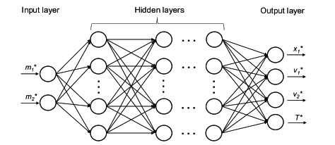
Figure 1: The artificial neural network (ANN) model, where the input $(m_{1}^{*},m_{2}^{*})$ and output $(x_{1}^{*},v_{1}^{*},v_{2}^{*},T^{*})$ are the normalized data of $(m_{1},m_{2})$ and $(x_{1},v_{1},v_{2},T)$, respectively.

Without loss of generality, let us consider such a known BHH periodic orbit with the initial condition $x_{1}$=-1.325626981682458, $v_{1}$=-0.8933877752879044, $v_{2}$=-0.2885702941263346, the period $T=9.199307755830397$ and the rotation angel $\theta_{T}=0.383160887655628$ of the coordinate frame, where $m_{1}=m_{2}=m_{3}=1$. Using this periodic orbit as a starting point, we first follow Li, Li and Liao [18] to obtain only 36 periodic orbits for different masses in a small domain $m_{1}\in[0.95,1.00],m_{2}\in[1.00,1.05]$ (marked by $S_{1}$, with the mass increment $\Delta m_{1}=\Delta m_{2}=0.01$) by means of the numerical continuation method [40] and the Newton-Raphson method [37, 38, 39]. Firstly, using the periodic orbit with equal masses, the periodic orbits with different masses $m_{1}$ and $m_{2}=m_{3}=1$ can be obtained by means of the continuation method and the Newton-Raphson method. Secondly, using these periodic orbits with different masses $m_{1}$ and $m_{2}=m_{3}=1$ as starting points, we obtain periodic orbits with different $m_{2}$ by means of the continuation method and the Newton-Raphson method. Finally, we can obtain periodic orbits with the mass domain $m_{1}\in[0.95,1.00],m_{2}\in[1.00,1.05]$ and $m_{3}=1$. For details, please refer to Li, Li and Liao [18]. The return distance (deviation) of these periodic orbits is defined by

$$\delta_{T}=\sqrt{\sum_{i=1}^{3}\Big{(}\left|\bm{r}_{i}(T)-\bm{r}_{i}(0)\right|^{2}+\left|\dot{\bm{r}}_{i}(T)-\dot{\bm{r}}_{i}(0)\right|^{2}\Big{)}}$$

in the rotating frame of reference, where $T$ is the period. Note that all of the 36 periodic orbits satisfy the criteria $\delta_{T}<10^{-10}$. Besides, they all have the same family name, which is defined by the so-called “free group element” according to Montgomery’s topological method [8].

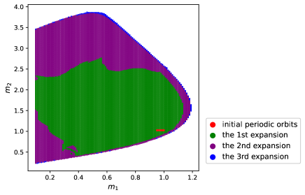
Figure 2: The periodic orbits found by expansion on the mass region. Red dot ($S_{1}$): initial periodic orbits; green dot ($S_{2}$): the first extrapolation/expansion ; purple dot ($S_{3}$): the second extrapolation/expansion; blue dot ($S_{4}$): the third extrapolation/expansion.

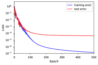
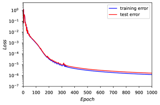
Figure 3: (a) Loss function of the neural network for the first training with 36 periodic orbits. (b) Loss function of the neural network for the second training with 17457 periodic orbits. Blue line: training error. Red line: test error.

Artificial neural network [43, 44, 45, 46] is a machine learning technique evolved from the idea of simulating the human brain, which can be used to perform statistical modelling. Compared with traditional regression approaches, the main advantages of ANN are as follows. First, the ANN does not require information about the complex nature of the underlying process to be explicitly expressed in mathematical form [47]. Besides, the ANN has capability of modelling more complex nonlinear relationships [48]. Therefore, generally speaking, the ANN is applicable across a wider range of problems than the traditional regression approaches. Especially, the ANN can easily deal with classification problems with complicated boundary [49]. Thus, we use the ANN in the following parts to model the relationship between the parameters of three-body problem and to classify the types of orbits and their stability.

In the next step, we use the ANN model to gain a relation between the input vector ($m_{1}$, $m_{2}$) and the output vector ($x_{1}$, $v_{1}$, $v_{2}$, $T$) of the periodic orbits. The ANN model we used here consists of multiple fully connected layers, say, one input layer, six hidden layers and one output layer. The number of neurons for the input layer, the hidden layers and the output layer is 2, 1024 and 4, respectively, as shown in Figure 1. We use the optimization algorithm AMSGrad [50] as an optimizer to minimize the mean square error for training the ANN model. At beginning, we use the results of the 36 known periodic orbits gained by means of the numerical continuation method [40] and the Newton-Raphson method [37, 38, 39] as the training set to train the ANN model. The trained ANN model provides us a kind of relationship (expressed by ${\cal F}_{1}$) between $(m_{1},m_{2})$ and $(x_{1},v_{1},v_{2},T)$, which can be further used to predict the initial conditions $x_{1}$, $v_{1}$, $v_{2}$ and the period $T$ of candidates (i.e. possible periodic orbits) for various masses ($m_{1},m_{2}$) outside of the original small domain $S_{1}=\left\{(m_{1},m_{2}):m_{1}\in[0.95,1.00],m_{2}\in[1.00,1.05]\right\}$. Using the neural network’s predictions as the initial guesses for the Newton-Raphson method, we first obtain the periodic orbits with various $m_{2}$ when $m_{1}=1$, and with various $m_{1}$ when $m_{2}=1$ in order to give a reference of the mass region of possible candidates. Then, we set the candidates of periodic orbits within the mass region $(m_{1},m_{2})\in[0.1,1.2),[0.4,2.8))$ with $\Delta m=0.01$ and exclude the mass region where the periodic orbits have been found. Finally, we find the 17421 new periodic orbits (66.1$\%$) within this region of 26364 candidates with $\delta_{T}<10^{-10}$ for various $(m_{1},m_{2})$ outside of $S_{1}$, which are marked in green in Figure 2 and expressed by $S_{2}$. In the same way, we further use the results of all (i.e. 36 + 17421 = 17457) known periodic orbits as a training set to train our ANN model so as to gain a better relationship ${\cal F}_{2}$ between ($m_{1}$, $m_{2}$) and ($x_{1}$, $v_{1}$, $v_{2}$, $T$) for extrapolation/expansion outside of the mass domain. We set the candidates of periodic orbits within the mass domain $(m_{1},m_{2})\in([0.1,1.2),[0.2,3.9))$ with $\Delta m=0.01$ and exclude the mass region where the periodic orbits have been found. Finally, we find the new 11473 periodic orbits marked in purple in Figure 2 and expressed by $S_{3}$ about 49.4$\%$ of all the 23243 candidates. Similarly, we use the results of all (i.e. 36 + 17421 + 11473 = 28930 ) known periodic orbits as the training set to further train our ANN model so as to give a relationship ${\cal F}_{3}$ between $(m_{1},m_{2})$ and $(x_{1},v_{1},v_{2},T)$. The chosen mass region $(m_{1},m_{2})$ of possible candidates is just beyond the boundary of previous obtained periodic orbits, where the horizontal or vertical distance from the $(m_{1},m_{2})$ to the boundary is less than $7\Delta m(\Delta m=0.01,m_{1}>0.1,m_{2}>0.1)$. Then, we find the 220 new periodic orbits as marked in blue in Figure 2 and expressed by $S_{4}$, only about 7.1$\%$ out of all the 3104 candidates. This indicates that we come to the boundary of the mass domain $(m_{1},m_{2})$ where the periodic orbits exit. In other words, there are no periodic orbits beyond that boundary. Thus, we find the nearly largest mass domain $S^{*}=S_{1}\cup S_{2}\cup S_{3}\cup S_{4}$ for the existence of periodic orbits with some similar properties.

Note that, for each training, we have examined that there is no overfitting phenomenon before we use the neural network for further prediction. As we randomly divide the whole dataset into the training set (90$\%$) and test set (10$\%$), and find that there is no distinct difference between the errors of these two sets. Then, we train the ANN with all the data including the training and test set to make the best use of the known data for further prediction. For example, for the first training, we randomly divide the dataset with 36 examples into training set (90$\%$) and test set (10$\%$). The loss function of training is shown in Fig. 3(a). The loss is defined as the mean squared error of the standardized data. The mean relative errors in the training set and test set are about $8.3\times 10^{-7}$ and $5.1\times 10^{-5}$, respectively. We find that as the training epoch increases, the error in the test set first decreases and then converges. It is not the phenomenon of overfitting where the loss function of test set first decreases and then increases. As the number of examples is limited, the test error is small while not as small as the training error. Then, we combine the test set into the training set to make use of all the data and use it for further extrapolation prediction. Note that, unlike the traditional use of the ANN, we apply the ANN model here to make extrapolation predictions of periodic orbits. As for the prediction error of extrapolation for $(x_{1},v_{1},v_{2},T)$, we calculate the mean relative error by comparing the ANN’s predictions with the “exact” results which are obtained by modifying the ANN’s predictions via the Newton-Raphson method. The mean relative error of the ANN’s extrapolation is about 0.05 for the first expansion of 17421 new periodic orbits. For the second training with 17457 (=17421+36) periodic orbits, we randomly divide the whole dataset into the training set (90%) and test set (10%). The loss function is shown in Fig. 3(b). The mean relative errors in the training set and test set are about $2.2\times 10^{-5}$ and $2.3\times 10^{-5}$, respectively. Thus, as the number of data is sufficient, the difference between the errors of training set and test set is very close. Then, we train all the 17457 examples for further prediction. The same approach is repeated in the similar way until no periodic orbits can be found by the ANN’s extrapolation prediction. The mean relative error of the ANN’s extrapolation prediction for the second and third expansion are about 0.009 and 0.00007, respectively. As shown in Figure 2, starting from the 36 periodic orbits in the original small domain $(m_{1},m_{2})\in S_{1}$ (marked in red), we totally gain the 29150 periodic orbits in the mass domain $(m_{1},m_{2})\in S^{*}=S_{1}\cup S_{2}\cup S_{3}\cup S_{4}$ by the three times extrapolations/expansions. Finally, training our ANN model by using all (i.e. 29150) these known results as a training set, we obtain a relationship ${\cal F}^{*}$ between $(m_{1},m_{2})\in S^{*}$ and ($x_{1}$, $v_{1}$, $v_{2}$, $T$), which can give the ANN’s predictions of periodic orbits for arbitrary values of $(m_{1},m_{2})\in S^{*}$ in the accuracy level of $10^{-4}$ for the return distance (deviation) $\delta_{T}$. All of these ANN’s predictions of periodic orbits are accurate enough for normal use, although their accuracy can be further modified to arbitrary level by means of the the Newton-Raphson method via the CNS and multiple-precision (MP), as mentioned below. Note that the mass domain $(m_{1},m_{2})$ with the periodic orbits becomes larger and larger, i.e. from $S_{1}$ to $S_{1}\cup S_{2}$ to $S_{1}\cup S_{2}\cup S_{3}$ to $S^{*}=S_{1}\cup S_{2}\cup S_{3}\cup S_{4}$, and the relationship between $(m_{1},m_{2})$ and ($x_{1}$, $v_{1}$, $v_{2}$, $T$) becomes better and better, from ${\cal F}_{1}$ to ${\cal F}_{2}$ to ${\cal F}_{3}$ to ${\cal F}^{*}$, implying that our ANN model becomes wiser and wiser!

Obviously, the smaller the return distance (deviation) $\delta_{T}$ is, the more accurate the periodic orbit given by the numerical strategy. Note that $\delta_{T}=0$ exactly corresponds to a closed-form periodic orbit. But unfortunately, except the Euler - Lagrange family, nearly all known periodic orbits of three-body systems were gained by numerical methods, and this fact is consistent with Poincaré’s famous proof of the non-existence of the uniform first integral of three-body systems [2]. It is found that, since the CNS and the MP (multiple precision) are used in our numerical strategy, the return distance (deviation) $\delta_{T}$ of these periodic orbits can be reduced to any given value, say, the initial conditions $(x_{1},v_{1},v_{2})$ and the period $T$ of these relatively periodic orbits can be at arbitrary level of precision, i.e. as accurate as one would like, as long as the performance of supercomputer is good enough.

In the present work, we use the ANN model as it is capable of modelling the complex nonlinear relationship, compared with the traditional approaches such as the linear model or two-dimensional regression. In the first training with 32 data, as the data is limited and the relationship is simple, the traditional approaches indeed have smaller mean relative errors in the test set, as shown in Table 1. However, in the second training with 17457 data when the data is sufficient and the relationship between the outputs and the inputs becomes more complex, the ANN model has better performance with smaller error in the test set than the linear model and the two-dimensional regression, as shown in Table 2. It reflects that one of the advantages of ANN is its ability to model more complex relationship. Thus, the ANN can be applicable across a wider range of problems.

Table 1: Mean relative errors of different models for the first training with 36 data.

  Model Training set (32 data) Test set (4 data) Linear model 3.09$\times 10^{-5}$ 3.40$\times 10^{-5}$ Two-dimensional interpolation 1.95$\times 10^{-7}$ 2.51 $\times 10^{-7}$ ANN 8.32 $\times 10^{-7}$ 5.11 $\times 10^{-5}$  

Table 2: Mean relative errors of different models for the second training with 17457 data.

  Model Training set (15711 data) Test set (1746 data) Linear model $1.54\times 10^{-2}$ $1.54\times 10^{-2}$ Two-dimensional interpolation $2.49\times 10^{-3}$ $2.49\times 10^{-3}$ ANN $2.18\times 10^{-5}$ $2.26\times 10^{-5}$  

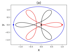
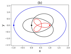
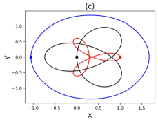
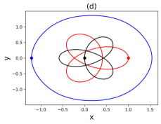
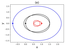
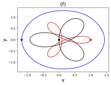
Figure 4: The relatively periodic BHH satellites orbits of the three-body system with various masses $m_{1}$ and $m_{2}$ in a rotating frame of reference. The corresponding physical parameters are given by ANN in Table 3. Blue line: body-1; red line: body-2; black line: body-3.

Table 3: Initial conditions and periods $T$ predicted by our trained ANN model for the six examples of BHH satellites with various masses $m_{1}$ and $m_{2}$ in case of $\bm{r}_{1}(0)=(x_{1},0)$, $\bm{r}_{2}(0)=(1,0)$, $\bm{r}_{3}(0)=(0,0)$, $\dot{\bm{r}}_{1}(0)=(0,v_{1})$, $\dot{\bm{r}}_{2}(0)=(0,v_{2})$, $\dot{\bm{r}}_{3}(0)=(0,-(m_{1}v_{1}+m_{2}v_{2})/m_{3})$, where $m_{i}$, $x_{i}$ and $v_{i}$ are the mass, initial position and velocity of the $i$-th body, respectively, with the same rotation angle $\theta=0.38316088765562$ of the reference frame for relatively periodic orbits.

  Case $m_{1}$ $m_{2}$ $x_{1}$ $v_{1}$ $v_{2}$ $T$ (a) 1.0124 0.9968 -1.32962 -0.88963 -0.28501 9.2111 (b) 0.5312 2.2837 -0.97138 -1.37584 -0.34528 7.0421 (c) 0.8056 2.0394 -1.05795 -1.24044 -0.26723 7.4389 (d) 0.3916 0.8341 -1.21503 -1.00328 -0.53749 9.2807 (e) 0.1472 3.4219 -0.80027 -1.74811 -0.42176 5.8793 (f) 0.8413 1.4155 -1.17777 -1.05903 -0.29934 8.3444  

The relationship ${\cal F}^{*}$ between $(m_{1},m_{2})\in S^{*}$ and $(x_{1},v_{1},v_{2},T)$ given by the ANN model is fundamentally different from the set of the original 29150 periodic orbits in the following aspects.

1. For arbitrary values of $(m_{1},m_{2})\in S^{*}$, ${\cal F}^{*}$ can always give a good enough prediction of the initial condition $(x_{1},v_{1},v_{2})$ and the period $T$ of the corresponding periodic orbit, which can be used as a starting point to gain a more accurate periodic orbit with a tiny return distance (deviation) $\delta_{T}<10^{-10}$.

2. For each prediction of a periodic orbit given by our ANN model for arbitrary values of $(m_{1},m_{2})\in S^{*}$, we can always modify it by means of the Newton-Raphson method [37, 38, 39], until a very accurate periodic orbit with $\delta_{T}<10^{-60}$ is gained. For examples, for the randomly chosen masses $m_{1}=0.550073$ and $m_{2}=1.738802$, the initial condition and period of the periodic orbit predicted by ${\cal F}^{*}$ is $x_{1}=-1.0509$, $v_{1}=-1.2291$, $v_{2}=-0.3751$ and $T=7.7189$. The return distance $\delta_{T}$ of this predicted periodic orbit is about $6\times 10^{-4}$, which can be reduced to $10^{-60}$ by means of the Newton-Raphson method [37, 38, 39] and the CNS, with the initial condition and period in accuracy of hundred significant digits:

   $$x_{1}=-1.0509175496041811604923698392786632425650672636140394304186656973,$$

   $$v_{1}=-1.2291270518667041014360821708612407200218851479344331903064815068,$$

   $$v_{2}=-0.37510727670051981894849679865106213490791658967297597038682248759,$$

   $$T=+7.7189475555888051714951891045174205372467192448577195610635970572.$$ (4)

   Note that the prediction given by our ANN model are in the accuracy of four significant digits. Similarly, we randomly check one thousand cases of $(m_{1},m_{2})\in S^{*}$, and found that, in every case, we indeed can always gain a periodic orbit with a quite tiny return distance (deviation) $\delta_{T}<10^{-60}$. All of these suggest that, statistically speaking, for arbitrary mass values $(m_{1},m_{2})\in S^{*}$, every prediction given by our ANN model could lead to a periodic orbit that could be in arbitrary accuracy as long as the performance of computer is good enough.

3. It is found that the mean absolute errors of predictions for randomly selected one thousand cases of $(m_{1},m_{2})\in S^{*}$ given by our trained ANN model ${\cal F}^{*}$ are in the level of $10^{-5}$ for the initial conditions $(x_{1},v_{1},v_{2})$ and $10^{-4}$ for the period $T$. Although we indeed can further gain a periodic orbit in accuracy of one hundred significant digits by means of the Newton-Raphson method [37, 38, 39] and the CNS, the periodic orbits predicted by our trained ANN model are good enough from practical viewpoint, since it is unnecessary to have so accurate trajectory in practice. For example, there also exits error in measurement for the actual astronomical observation. In practice, it is rather convenient to gain a periodic orbit for arbitrary masses $(m_{1},m_{2})\in S^{*}$ by means of the initial conditions $(x_{1},v_{1},v_{2})$ and period $T$ predicted by the trained ANN model, for example, as shown in Figure 4 for randomly chosen six different masses of $m_{1}$ and $m_{2}$. Compared with using the numerical continuation method to find a periodic orbit with arbitrary mass $(m_{1},m_{2})\in S^{*}$, using the neural network can directly provide a good enough prediction of periodic orbit in practice. While for the numerical continuation method, we need to modify the initial conditions by the Newton-Raphson method to give a good enough solution. Even if we aim to obtain the periodic orbits with high precision, the neural network can give more accurate initial solution for the Newton-Raphson method. Thus, our ANN model provides us great convenience in practice.

4. The ANN model can ceaselessly learn and thus be further modified when some new periodic orbits are gained, say, the trained ANN model could become wiser and wiser.

In summary, we illustrate that the trained ANN model can provide us accurate enough periodic orbits for arbitrary values of $(m_{1},m_{2})$ in an irregular domain $S^{*}$.

How accurate is a periodic orbit with return distance (deviation) $d_{T}<10^{-60}$ ? Let $\Delta x_{1}$ denote the dimensionless deviation of the initial position. Even if we use the diameter of universe $d_{u}$ = 930 light year = $8.8\times 10^{18}$ meter as the characteristic length $L$, we have the corresponding inaccuracy of the dimensional initial position $|\Delta x_{1}|d_{u}<10^{-41}$ meter, which is six order of magnitude smaller than the Planck length $l_{p}\approx 1.62\times 10^{-35}$ meter. Note that Planck length is a lower bound to physical proper length in any space-time: it is impossible to measure length scales smaller than the Planck length, according to Padmanabhan [51]. Besides, it should be emphasized that all of these periodic orbits are stable, say, a tiny disturbance does not increase exponentially. So, from physical view-point, a stable periodic orbit with return distance (deviation) $d_{T}<10^{-60}$ gained by numerical method is physically equivalent to $d_{T}=0$ that corresponds to an exact solution of periodic orbit in a closed-form.

Therefore, the high-performance computer and the machine learning play very important role in finding periodic orbits of three-body systems with arbitrary masses. It should be emphasized here that it is Turing [20, 21] who laid the foundations of modern computer and artificial intelligence (including machine learning).

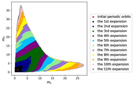
Figure 5: The relatively periodic orbits with the same rotation angle $\theta=0.0105056462558377$ of reference frame, found in each extrapolation/expansion on the various mass regions. Red dot: initial periodic orbits; black dot: 1st expansion; dark blue dot: 2nd expansion; dark green dot: the 3rd expansion. dark purple dot: the 4th expansion; light blue dot: the 5th expansion; light green dot: the 6th expansion; light purple dot: the 7th expansion; yellow dot: the 8th expansion; orange dot: the 9th expansion; pink dot: the 10th expansion; grey dot: the 11th expansion.

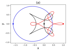
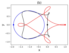
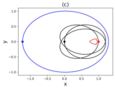
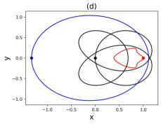
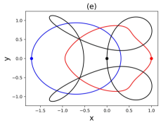
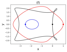
Figure 6: The relatively periodic BHH satellites orbits of the three-body system with various masses $m_{1}$ and $m_{2}$ in a rotating frame of reference. The corresponding physical parameters are given by ANN in Table 4. Blue line: body-1; red line: body-2; black line: body-3.

The above approach has general meaning. To show this point, let us further consider another BHH satellite periodic orbit with three equal masses $m_{1}=m_{2}=m_{3}=1$, $x_{1}$ = $-1.609965115714630$, $v_{1}=-0.6656909425824538$, $v_{2}=-0.1529561125709906$, the period $T=6.879203007710456$ and the rotation angel $\theta=0.0105056462558377$ of the reference frame (for relatively periodic orbits). At first, using this known periodic orbit as a starting point, we can obtain 36 periodic orbits with various masses in a small mass domain $m_{1}\in[1.0,1.5]$ and $m_{2}\in[1.0,1.5]$ (with mass increment $\Delta m_{1}=\Delta m_{2}=0.1$) by combining the numerical continuation method [40] and the Newton-Raphson method [37, 38, 39].

Similarly, we train a ANN model (with the same structure as mentioned above) by means of the initial conditions and periods of these 36 known periodic orbits and then use the trained ANN model to predict the initial conditions and periods of some candidates of possible periodic orbits outside the previous mass domain, while the initial conditions and periods of each candidate are modified by the Newton-Raphson method [37, 38, 39] so as to confirm whether or not the candidate is a periodic one, say, its return distance can be reduced to the tiny level of $10^{-10}$. The same process repeats 11 times, while the number of the known relatively periodic orbits becomes more and more, the mass domain becomes larger and larger, and the ANN model becomes wiser and wiser! Finally, we totally obtain 35895 relatively periodic orbits in a mass domain $\bar{S}^{*}$ whose area is about 1000 times larger than the initial one $m_{1}\in[1.0,1.5]$ and $m_{2}\in[1.0,1.5]$, as shown in Fig. 5.

Table 4: Initial conditions and periods $T$ of six examples of BHH satellites with various masses $m_{1}$ and $m_{2}$, predicted by our trained ANN model in case of $\bm{r}_{1}(0)=(x_{1},0)$, $\bm{r}_{2}(0)=(1,0)$, $\bm{r}_{3}(0)=(0,0)$, $\dot{\bm{r}}_{1}(0)=(0,v_{1})$, $\dot{\bm{r}}_{2}(0)=(0,v_{2})$, $\dot{\bm{r}}_{3}(0)=(0,-(m_{1}v_{1}+m_{2}v_{2})/m_{3})$, where $m_{i}$, $x_{i}$ and $v_{i}$ are the mass, initial position and velocity of the $i$-th body, respectively, with the same rotation angle $\theta=0.0105056462558377$ of the reference frame for relatively periodic orbits.

  No. $m_{1}$ $m_{2}$ $x_{1}$ $v_{1}$ $v_{2}$ $T$ (a) $1.0283$ $0.9879$ $-1.62064$ $-0.65955$ $-0.14784$ $6.9193$ (b) $1.5142$ $0.4968$ $-1.90809$ $-0.50283$ $-0.08614$ $8.2924$ (c) $2.9216$ $31.9067$ $-1.22892$ $-2.37239$ $0.09481$ $1.6822$ (d) $4.4143$ $18.6575$ $-1.32880$ $-1.86103$ $0.25507$ $2.3306$ (e) $10.3501$ $10.4522$ $-1.69797$ $-1.22777$ $0.86183$ $3.5607$ (f) $18.7011$ $4.2388$ $-2.51585$ $-0.53262$ $1.49754$ $5.9612$  

Similarly, we further train our ANN model by using the known 35895 relatively periodic orbits. To show the validation and accuracy of this ANN’s model, we randomly chose 1000 cases of arbitrary mass $(m_{1},m_{2})\in\bar{S}^{*}$, and it is found that the initial conditions and periods predicted by our trained ANN model can provide us good enough periodic orbits with a return distance $d_{T}$ in a tiny level of $10^{-3}$ (about 71$\%$), $10^{-4}$ (about 2$\%$), and $10^{-2}$ (about 27$\%$), which can be further decreased by means of the clean numerical simulation (CNS) and the Newton-Raphson method with multiple-precision (MP) until a very small return distance (such as $d_{T}<10^{-60}$) is satisfied. Thus, generally speaking, our trained ANN model can always give periodic orbits for an arbitrary mass $(m_{1},m_{2})\in S_{2}^{*}$, which is accurate enough from practical viewpoint. For example, randomly choosing six cases with various masses $m_{1}$ and $m_{2}$, where $(m_{1},m_{2})\in\bar{S}^{*}$, our ANN model can quickly predict their initial conditions and periods, as listed in Table 4, and give the corresponding trajectories in a satisfied level of accuracy, as shown in Fig 6. It is found that the differences between the periodic orbits predicted by the ANN’s model with $10^{-4}<d_{T}<10^{-2}$ and the “exact” ones further modified by the Newton-Raphson method and the multiple-precision (MP) with $d_{T}<10^{-60}$ are negligible for practical uses. Thus, our approach based on the ANN model has indeed general meanings.

3 Classification for orbits based on machine learning

Stability is an important property of periodic orbits, because only stable triple systems can be observed. We employ a theorem given by Kepela and Simó [52] to determine the linear stability of periodic orbits of three-body problem through the monondromy matrix [53]. It is found that all relatively periodic orbits for the first case with the rotation angle $\theta=0.3831608876556280$ are linearly stable. For the second case with the rotation angle $\theta=0.0105056462558377$, there are 16739 linearly stable periodic orbits among the 35895 computer-generated periodic orbits, as shown in Fig 7. Note that, the ANN can be applicable to deal with complicated classification problems [49]. We use the ANN to classify different types of orbits for different masses which have complex shapes of the boundary. We can give an ANN classifier model to classify the periodicity and stability of the orbits for arbitrary masses $m_{1}$ and $m_{2}$, especially for the masses nearly the boundary of each type. The orbits are classified into three categories: stable periodic orbits, unstable periodic orbits and non-periodic orbits, expressed by $[1,0,0]$, $[0,1,0]$ and $[0,0,1]$, respectively. The ANN classifier model consists of eight fully connected layers with one input layer, six hidden layers and one output layer. The numbers of neurons for input layer, hidden layers and output layer are 2, 256 and 3, respectively. Different from the above-mentioned ANN regression model, the activation function of the ANN classifier model is softmax function. The loss function is cross entropy. As shown in Fig 8, for the first case, the mass domain of 3128 non-periodic orbits are outside the boundary of periodic orbits. The numbers of stable periodic orbits, unstable periodic orbits and non-periodic orbits are 29150, 0 and 3128, respectively. For the second case, the mass domain of 5900 non-periodic orbits are outside the boundary of periodic orbits. The numbers of stable periodic orbits, unstable periodic orbits and non-periodic orbits are 16739, 19156 and 5900, respectively. For each case, the whole dataset is randomly divided into three sets, the training set (90%), validation set (5%) and test set (5%).

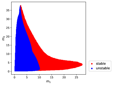
Figure 7: The linear stability of the relatively periodic orbits in the second case with the rotation angle $\theta=0.0105056462558377$. Red domain: stable; blue domain: unstable.

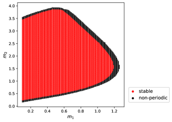
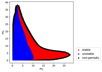
Figure 8: The linear stability and periodicity of the orbits for the first case (a) and the second case (b). Red dot: linear stable; blue dot: unstable; black dot: non-periodic.

Table 5: Confusion matrix for the ANN predictions in test set of the first case.

  Type Stable periodic orbits Non-periodic orbits Stable periodic orbits 1475 2 Non-periodic orbits 0 137  

Table 6: Confusion matrix for the ANN predictions in test set of the second case.

  Type Stable periodic orbits Unstable periodic orbits Non-periodic orbits Stable periodic orbits 846 1 5 Unstable periodic orbits 1 943 2 Non-periodic orbits 1 0 291  

The early stopping [54] is used when training, and we save the ANN model with the maximum accuracy in the validation set. The test set is used to verify the generalization capability of the ANN model. For the first case, the accuracies of the training set, validation set and test set are about $99.98\%$, $99.94\%$ and $99.94\%$ , respectively. And the macro F1-scores [55] of the training set, validation set and test set are about 0.9995, 0.9983 and 0.9980, respectively. For the second case, the accuracies of the training set, validation set and test set are about $99.62\%$, $99.57\%$ and $99.52\%$, respectively. And the macro F1-scores of the training set, validation set and test set are about 0.9941, 0.9935 and 0.9932, respectively. As the accuracies and F1-scores of the training set and test set are close, overfitting doesn’t exist in these two cases. The confusion matrixes for the ANN predictions in the test sets of the first and second case are as shown in Table 5 and 6, respectively, which illustrate the good performances of the ANN. Therefore, we can use the ANN classifier to predict the periodicity and stability of orbits for any given masses in each case.

4 A roadmap of searching for periodic orbits of three-body problem

The successful examples mentioned above suggest us a general road map for finding new periodic orbits of three-body system (in case of $m_{3}=1$) with the same “free group element” (word) given by Montgomery’s topological method [8]:

1. For a three-body system with three or two equal masses, first find candidates of the initial conditions for possible periodic orbits by means of the grid search method, and then modify these candidates by means of the Newton-Raphson method [37, 38, 39], until a satisfied periodic orbit with a tiny enough return distance (deviation) is obtained;

2. Given a known periodic orbit, use it as a starting point to gain a few of new periodic orbits with various masses in a small domain of mass $(m_{1},m_{2})$ by combining the numerical continuation method [40] and the Newton-Raphson method [37, 38, 39]. The initial conditions and periods of all these known periodic orbits form a training set for a ANN model.

3. For a given training set in a mass domain of $(m_{1},m_{2})$, train the ANN model to predict initial conditions and periods so that some new periodic orbits outside of the previous mass domain of $(m_{1},m_{2})$ could be found by modifying these predictions via the Newton-Raphson method [37, 38, 39]. Then, combining the results of these new periodic orbits with the previous training set, we further have a new training set with more elements, which could further provide us some new periodic orbits in a even larger mass domain of $(m_{1},m_{2})$ in a similar way, outside of the previous one. The same process can repeat again and again, so that more and more periodic orbits are found in a larger and larger mass domain of $(m_{1},m_{2})$, and the ANN model becomes wiser and wiser, until quit few or no new periodic orbits can be found in a larger domain of $(m_{1},m_{2})$. Finally, we have a trained ANN model ${\cal F}^{*}$ of all periodic orbits in the final mass domain $(m_{1},m_{2})\in S^{*}$.

4. Randomly choose hundreds or thousands of arbitrary masses $(m_{1},m_{2})\in S^{*}$. For each case, check whether or not the trained ANN model ${\cal F}^{*}$ could give an accurate enough prediction, and in addition whether or not the corresponding return distance (deviation) could be indeed reduced to $10^{-60}$. If yes, then the ANN model ${\cal F}^{*}$ can provide a good enough prediction of periodic orbits in the domain $(m_{1},m_{2})\in S^{*}$, from practical viewpoint.

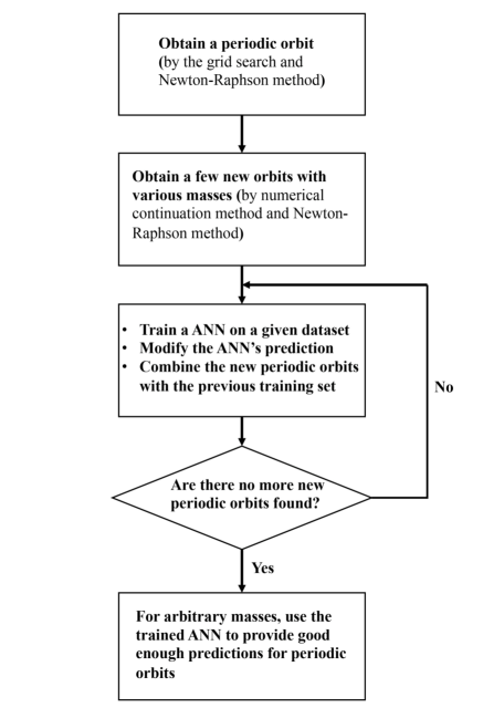
Figure 9: A roadmap for searching the periodic orbits of three-body problem

The pipeline for searching the periodic orbits of three-body problem is shown in Fig. 9. Note that it is better to use the CNS as integrator so as to guarantee the reliability and convergence of computer-generated trajectories of chaotic three-body system under arbitrary initial conditions in a required long interval of time. Besides, the periodicity and stability of orbits for arbitrary masses $m_{1}$ and $m_{2}$ can be well predicted by an ANN classifier model.

5 Concluding remarks and discussions

The famous three-body problem can be traced back to Newton in 1687, but quite few families of periodic orbits were found in 300 years thereafter. As proved by Poincarè, the first integral does not exist for three-body systems, which implies that numerical approach had to be used in general.

Artificial neural network [43, 44, 45, 46] is a machine learning technique evolved from simulating the human brain, which has been widely proved to be rather powerful. Compared with the traditional regression approaches, the ANN has many advantages. First, the ANN does not require information about the complex nature of the underlying process to be explicitly expressed in mathematical form [47]. Besides, generally speaking, the ANN can handle more complex nonlinear relationships than the traditional regression approaches [48], so that the ANN is applicable across a wider range of problems. Especially, the ANN can be easily applied to deal with classification problems with complicated boundary [49]. Therefore, we use the ANN here to model the relationship between the parameters of three-body problem and to classify the types of orbits and their stability.

In this paper, we propose an effective approach and roadmap to numerically gain planar periodic orbits of three-body systems with arbitrary masses by means of machine learning based on an artificial neural network (ANN) model. Given any a known periodic orbit as a starting point, this approach can provide more and more periodic orbits (of the same family name) with variable masses, while the mass domain having periodic orbits becomes larger and larger, and the ANN model becomes wiser and wiser. Finally we have an ANN model trained by means of all obtained periodic orbits of the same family, which provides a convenient way to give accurate enough periodic orbits with arbitrary masses for physicists and astronomers. In addition, the periodicity and stability of orbits for arbitrary masses can be well predicted by an ANN classifier model.

It must be emphasized that high performance computer and artificial intelligence (including machine learning) play important roles in solving periodic orbits of triple systems. Today, nothing can prevent us from obtaining massive periodic solutions of three-body problem. This is due to the great contributions of some great mathematicians, scientists and engineers in more than three hundred years! Especially, it is Poincaré [2] who made a historical turning point by proving the non-existence of the uniform first integral of triple system, which implies that we had to use numerical approach in general. It is Turing [20, 21] who published his epoch-making papers that became the foundation of modern computer and artificial intelligence. It is Von Neumann [22] who proposed the so-called “Von Neumann - Machine” for modern computer. It is Jack S. Kilby, the winner of Nobel prize for physics in 2000, who took part in the invention of the integrated circuit. And so on. The famous three-body problem might be an excellent example to illustrate the importance of inventing new tools for human being to better understand and explore the nature.

The approach and roadmap mentioned in this paper has general meanings. Note that thousands of families of periodic orbits of triple systems with three or two equal masses have currently been found (for example, please visit the website https://github.com/sjtu-liao/three-body). Using any of them as a starting point, we can similarly gain a trained ANN model to give accurate enough predictions of periodic orbits of the same family of triple system in a corresponding mass domain. All of these might form a massive data base for periodic orbits of triple systems, which should be helpful to enrich and deepen our understandings about the famous three-body systems. Besides, hopefully, some physical laws, such as generalized Kepler’s law [9] for periodic orbits of triple systems with arbitrary masses, could be found in future by analysing these massive data by means of machine learning.

Note also that nearly all known periodic orbits of triple systems are planar, i.e. two-dimensional. In theory, the same ideas mentioned in this paper can be used to search for periodic orbits of triple systems in three dimensions. Although, according to our results reported here and in the previous papers [10, 18], given a pair $(m_{1},m_{2})$, there is only one possible set $(x_{1},v_{1},v_{2},T)$ that would lead to a periodic orbit of the three-body problem, it should be interesting to investigate whether there exist bifurcations of periodic orbits in future.

Data Availability Statements

The data and the code related to this paper can be seen in the website (https://github.com/sjtu-liao/three-body), including the trained ANN models of the two cases, all the periodic orbits found (also including those reported in [9, 10, 18]), the code to train the ANN and use the ANN to predict the periodic orbits, and the code to train the ANN for classifying the orbits.

Author contributions

S.J.L. provided the main ideas and wrote the manuscript. X.M.L. calculated the periodic orbits. Y.Y. analysed the results by means of machine learning based on an ANN model. All authors contributed to the discussion and revision of the final manuscript.

Declaration of competing interest

The authors declare that they have no competing financial interests.

Appendix – Direct search for periodic orbits with arbitrary masses

The phase space of the planar three-body problem has 12 dimensions. The grid searching method suffers the curse of dimensionality in such high dimensions. In order to reduce the dimensionality of the searching space, we can fix some parameters of initial conditions. Since the collinear instant of three bodies is common in the three-body system, it is reasonable to consider three bodies are in a line at the start of periodic orbits. The three bodies are in a line for the BHH family of periodic orbits: $\bm{r}_{1}(0)=(x_{1},0)$, $\bm{r}_{2}(0)=(x_{2},0)$, $\bm{r}_{3}(0)=(x_{3},0)$, and their initial velocities are orthogonal to the line: $\dot{\bm{r}}_{1}(0)=(0,v_{1})$, $\dot{\bm{r}}_{2}(0)=(0,v_{2})$, $\dot{\bm{r}}_{3}(0)=(0,v_{3})$.

According to the scaling law of the three-body system [18], we can fix $x_{2}=1$ and $x_{3}=0$. Without loss of generality, we assume momentum of the system is equal to zero, thus $v_{3}=-(m_{1}v_{1}+m_{2}v_{2})/m_{3}$.

The approximated initial conditions and periods of periodic orbits can be obtained through grid searching method, then these approximated periodic orbits will be corrected by means of the Newton-Raphson method [37, 38, 39] and the clean numerical simulation (CNS) [31, 33, 35]. The differential equations of the planar three-body problem can be described as:

$$\dot{\bm{x}}=\bm{f}(\bm{x});\quad\bm{x}(0)=\bm{y},\quad\bm{x}\in\mathbb{R}^{12},$$ (5)

and $\bm{x}=\bm{x}(t,\bm{y})$, $t\in\mathbb{R}$, $\bm{x,y}\in\mathbb{R}^{12}$ is the solution of these equations, where $\bm{y}$ is the initial condition.

For the initial condition $\bm{y}$ and period $T$, a relative periodic orbit with a rotation angle $\theta$ means that

$$\bm{x}(T,\bm{y})-\bm{P}(\theta)\bm{y}=0,$$ (6)

where $\bm{P}(\theta)$ is the rotation matrix.

Now we correct the approximated initial conditions and periods of periodic orbits. Let us assume the approximated initial conditions and periods are $(\bm{y}_{i},T_{i})$ at $i$-th step. To improve accuracy of the approximated initial conditions and periods, the corrections of initial conditions and periods $(\Delta\bm{y}_{i},\Delta T_{i})$ should be satisfied the following equations:.

$$\bm{x}(T_{i}+\Delta T_{i},\bm{y}_{i}+\Delta\bm{y}_{i})-\bm{P}(\theta)(\bm{y}_{i}+\Delta\bm{y}_{i})=0.$$ (7)

Using the first order Taylor approximation of the above equations, we have

$$\bm{x}(T_{i},\bm{y}_{i})-\bm{P}(\theta)\bm{y}_{i}+\left(\frac{\partial\bm{x}}{\partial\bm{y}}-\bm{P}(\theta)\right)\Delta\bm{y}_{i}+\frac{\partial\bm{x}}{\partial t}\Delta T_{i}=0,$$ (8)

where $\bm{P}(\theta)$ is the rotation matrix, $\bm{M}=\partial\bm{x}/\partial\bm{y}$ is the solution of variational equations. $\partial\bm{x}/\partial t$ is the derivative of the solution at $t=T_{i}$, i.e., $\bm{f}(\bm{y}_{T_{i}})$, where $\bm{y}_{T_{i}}=\bm{x}(T_{i},\bm{y}_{i})$.

Finally, we obtain the following linear system:

$$\left(\begin{array}[]{cc}\bm{M}-\bm{P}(\theta)&\bm{f}(\bm{y}_{T_{i}})\\ \end{array}\right)\left(\begin{array}[]{c}\Delta\bm{y}_{i}\\ \Delta T_{i}\end{array}\right)=\left(\begin{array}[]{c}\bm{P}(\theta)\bm{y}_{i}-\bm{y}_{T_{i}}\\ \end{array}\right).$$ (9)

Then the correction of initial conditions and periods of periodic orbits can be computed through solving these linear equations. As we fix some parameters of the initial conditions, only variables $x_{1}$, $v_{1}$, $v_{2}$ and $T$ will be modified. Then we have linear equations $\bm{A}\bm{z}=\bm{b}$, where $\bm{A}$ is a $12\times 4$ matrix, $\bm{z}=(\Delta x_{1}\;\Delta v_{1}\;\Delta v_{2}\;\Delta T)^{\intercal}$ is a 4-vector and $\bm{b}$ is a 12-vector. Since the matrix $\bm{A}$ is not a square matrix, we solve this system by means of the least-norm method with SVD [56].

References

- [1] I. Newton, Philosophiæ naturalis principia mathematica (Mathematical Principles of Natural Philosophy), London: Royal Society Press, 1687.
- [2] J. H. Poincaré, Sur le probléme des trois corps et les équations de la dynamique. Divergence des séries de m. Lindstedt, Acta Math. 13 (1890) 1–270.
- [3] R. Broucke, On relative periodic solutions of the planar general three-body problem, Celestial Mechanics 12 (4) (1975) 439 – 462.
- [4] R. Broucke, D. Boggs, Periodic orbits in the planar general three-body problem, Celestial mechanics 11 (1) (1975) 13–38.
- [5] J. D. Hadjidemetriou, The stability of periodic orbits in the three-body problem, Celestial Mechanics 12 (3) (1975) 255–276.
- [6] M. Hénon, A family of periodic solutions of the planar three-body problem, and their stability, Celestial mechanics 13 (3) (1976) 267–285.
- [7] C. Moore, Braids in classical dynamics, Phys. Rev. Lett. 70 (1993) 3675–3679.
- [8] R. Montgomery, The N-body problem, the braid group, and action-minimizing periodic solutions, Nonlinearity 11 (2) (1998) 363.
- [9] X. Li, S. Liao, More than six hundred new families of Newtonian periodic planar collisionless three-body orbits, Science China - Physics, Mechanics & Astronomy 60 (12) (2017) 129511.
- [10] X. Li, Y. Jing, S. Liao, Over a thousand new periodic orbits of a planar three-body system with unequal masses, Publications of the Astronomical Society of Japan 70 (4) (2018) 64.
- [11] B. Sun, Kepler’s third law of n-body periodic orbits in a newtonian gravitation field, Science China Physics, Mechanics & Astronomy 61 (5) (2018) 1–4.
- [12] J. A. Kwiecinski, A. Kovacs, A. L. Krause, F. B. Planella, R. A. Van Gorder, Chaotic dynamics in the planar gravitational many-body problem with rigid body rotations, International Journal of Bifurcation and Chaos 28 (2018) 1830013.
- [13] N. C. Stone, N. W. Leigh, A statistical solution to the chaotic, non-hierarchical three-body problem, Nature 576 (7787) (2019) 406–410.
- [14] X. Li, S. Liao, Collisionless periodic orbits in the free-fall three-body problem, New Astronomy 70 (2019) 22–26.
- [15] K. Lin, X. Zhao, C. Zhang, T. Liu, B. Wang, S. Zhang, X. Zhang, W. Zhao, T. Zhu, , A. Wang, Gravitational waveforms, polarizations,response functions, and energy losses of triple systems in einstein-aether theory, Physical Review D 99 (2019) 023010.
- [16] K. Tanikawa, M. M. Saito, S. Mikkola, A search for triple collision orbits inside the domain of the free-fall three-body problem, Celestial Mechanics and Dynamical Astronomy 131 (2019) 24.
- [17] E. I. Abouelmagd, J. L. G. Guirao, A. K. Pal, Periodic solution of the nonlinear Sitnikov restricted three-body problem, New Astronomy 75 (2020) 101319.
- [18] X. Li, X. Li, S. Liao, One family of 13315 stable periodic orbits of non-hierarchical unequal-mass triple systems, Science China - Physics, Mechanics & Astronomy 64 (1) (2021) 219511.
- [19] E. Lorenz, Deterministic non-periodic flow, Journal of the Atmospheric Sciences 20 (2) (1963) 130–141.
- [20] A. Turing, On computable numbers, with an application to the Entscheidungs problem, Proc. London Maths. Soc. 42 (1936) 230–265.
- [21] A. Turing, Computing machinery and intelligence, Mind 50 (1950) 433–460.
- [22] J. Von Neumann, The Computer and the Brain, Yale University Press, 1958.
- [23] M. Šuvakov, V. Dmitrašinović, Three classes of Newtonian three-body planar periodic orbits, Phys. Rev. Lett. 110 (2013) 114301.
- [24] E. Lorenz, Computational chaos-a prelude to computational instability, Physica D: Nonlinear Phenomena 35 (3) (1989) 299–317.
- [25] E. Lorenz, Computational periodicity as observed in a simple system, Tellus A 58 (2006) 549 – 557.
- [26] J. Li, Q. Peng, J. Zhou, Computational uncertainty principle in nonlinear ordinary differential equations (i), Science in China 43 (2000) 449–460.
- [27] J. Li, Q. Zeng, J. Chou, Computational uncertainty principle in nonlinear ordinary differential equations, Science in China Series E: Technological Sciences 44 (1) (2001) 55–74.
- [28] J. Teixeira, C. A. Reynolds, K. Judd, Time step sensitivity of nonlinear atmospheric models: numerical convergence, truncation error growth, and ensemble design, Journal of the Atmospheric Sciences 64 (1) (2007) 175–189.
- [29] L. Yao, D. Hughes, Comment on“computational periodicity as observed in a simple system” by Edward N. Lorenz (2006), Tellus A 60 (2008) 803 – 805.
- [30] N. Chandramoorthy, Q. Wang, On the probability of finding nonphysical solutions through shadowing, J. Comput. Phys. 440 (2021) 110389.
- [31] S. Liao, On the reliability of computed chaotic solutions of non-linear differential equations, Tellus A 61 (4) (2009) 550–564.
- [32] S. Liao, Physical limit of prediction for chaotic motion of three-body problem, Communications in Nonlinear Science and Numerical Simulation 19 (3) (2014) 601–616.
- [33] S. Liao, P. Wang, On the mathematically reliable long-term simulation of chaotic solutions of Lorenz equation in the interval [0,10000], Sci. China - Phys. Mech. Astron. 57 (2014) 330 – 335,.
- [34] S. Liao, X. Li, On the inherent self-excited macroscopic randomness of chaotic three-body systems, Int. J. Bifurcation & Chaos 25 (2015) 1530023 (11 page).
- [35] T. Hu, S. Liao, On the risks of using double precision in numerical simulations of spatio-temporal chaos, Journal of Computational Physics 418 (2020) 109629.
- [36] S. Liao, S. Qin, Ultra-chaos: an insurmountable objective obstacle of reproducibility and replication, Adv. Appl. Math. Mech. 14 (4) (2022) 799–815.
- [37] S. C. Farantos, Methods for locating periodic orbits in highly unstable systems, Journal of Molecular Structure: THEOCHEM 341 (1) (1995) 91 – 100.
- [38] M. Lara, J. Pelaez, On the numerical continuation of periodic orbits - an intrinsic, 3-dimensional, differential, predictor-corrector algorithm, Astronomy and Astrophysics 389 (2) (2002) 692–701.
- [39] A. Abad, R. Barrio, A. Dena, Computing periodic orbits with arbitrary precision, Phys. Rev. E 84 (2011) 016701.
- [40] E. L. Allgower, K. Georg, Introduction to numerical continuation methods, Vol. 45, SIAM, 2003.
- [41] M. R. Janković, V. Dmitrašinović, Angular momentum and topological dependence of Kepler’s third law in the Broucke-Hadjidemetriou-Hénon family of periodic three-body orbits, Phys. Rev. Lett. 116 (2016) 064301.
- [42] M. R. Janković, V. Dmitrašinović, M. Šuvakov, A guide to hunting periodic three-body orbits with non-vanishing angular momentum, Computer Physics Communications 250 (2020) 107052.
- [43] M. H. Hassoun, et al., Fundamentals of artificial neural networks, MIT press, 1995.
- [44] M. Gevrey, I. Dimopoulos, S. Lek, Review and comparison of methods to study the contribution of variables in artificial neural network models, Ecological modelling 160 (3) (2003) 249–264.
- [45] R. Andrews, J. Diederich, A. B. Tickle, Survey and critique of techniques for extracting rules from trained artificial neural networks, Knowledge-based systems 8 (6) (1995) 373–389.
- [46] O. I. Abiodun, A. Jantan, A. E. Omolara, K. V. Dada, N. A. Mohamed, H. Arshad, State-of-the-art in artificial neural network applications: A survey, Heliyon 4 (11) (2018) e00938.
- [47] K. Sudheer, A. Gosain, K. Ramasastri, A data-driven algorithm for constructing artificial neural network rainfall-runoff models, Hydrological processes 16 (6) (2002) 1325–1330.
- [48] D. J. Livingstone, Artificial neural networks: methods and applications, Springer, 2008.
- [49] R. Bala, D. Kumar, Classification using ann: A review, Int. J. Comput. Intell. Res 13 (7) (2017) 1811–1820.
- [50] S. J. Reddi, S. Kale, S. Kumar, On the convergence of Adam and beyond, arXiv preprint arXiv:1904.09237.
- [51] T. Padmanabhan, Physical significance of Planck length, Annals of Physics 165 (1985) 38 – 58.
- [52] T. Kapela, C. Simó, Computer assisted proofs for nonsymmetric planar choreographies and for stability of the Eight, Nonlinearity 20 (5) (2007) 1241.
- [53] C. Simó, Dynamical properties of the figure eight solution of the three-body problem, Celestial Mechanics: Dedicated to Donald Saari for His 60th Birthday: Proceedings of an International Conference on Celestial Mechanics, December 15-19, 1999, Northwestern University, Evanston, Illinois 292 (2002) 209.
- [54] L. Prechelt, Early stopping-but when?, in: Neural Networks: Tricks of the trade, Springer, 1998, pp. 55–69.
- [55] W. Dimitrov, H. Lehmann, K. Kamiński, M. K. Kamińska, M. Zgórz, M. Gibowski, The hierarchical triple system DY Lyncis, Monthly Notices of the Royal Astronomical Society 466 (1) (2017) 2–10.
- [56] L. Trefethen, D. Bau III, Numerical Linear Algebra, Society for Industrial and Applied Mathematics, Philadelphia, PA, 1997.