Transverse charge distributions of the nucleon and their Abel images

Abstract

We investigate the two-dimensional transverse charge distributions of the transversely polarized nucleon. As the longitudinal momentum ($P_{z}$) of the nucleon increases, the electric dipole moment is induced, which causes the displacement of the transverse charge and magnetization distributions of the nucleon. The induced dipole moment of the proton reaches its maximum value at around $P_{z}\approx 3.2$ GeV due to the kinematical reason. We also investigate how the Abel transformations map the three-dimensional charge and magnetization distributions in the Breit frame onto the transverse charge and magnetization ones in the infinite momentum frame.

I Introduction

The electromagnetic (EM) structure of the nucleon has been one of the most important issues well over decades since Hofstadter’s experiments Hofstadter:1956qs (see a recent review Punjabi:2015bba and references therein). The EM form factors of the nucleon, which can be measured by electron-nucleon scattering, provide information on the three-dimensional (3D) charge and magnetization distributions for the nucleon in the Breit frame (BF). They have traditionally been obtained by the 3D Fourier transform Ernst:1960zza ; Sachs:1962zzc . However, this interpretation is true only when the size of a system is much larger than the Compton wavelength ($\lambdabar=\hbar/Mc$). This means that the definitions of the 3D charge and magnetization distributions are completely valid for nonrelativistic particles such as atoms and nuclei. On the other hand, the charge radius of the nucleon is approximately four times larger than the Compton wavelength, which indicates that the relativistic corrections are about 20 % for the distributions and about 10 % for the charge and magnetic radii of the nucleon. This indicates that the nucleon is per se a relativistic particle. In fact, Yennie et al. raised this point already many years ago Yennie:1957 . Recently, the criticisms on the 3D distributions of the nucleon have been renewed Burkardt:2000za ; Burkardt:2002hr ; Miller:2007uy ; Miller:2010nz ; Lorce:2020onh ; Jaffe:2020ebz . Because of these ambiguous relativistic corrections, the 3D charge and magnetization distributions cannot be interpreted as quantum-mechanical probability densities but can be understood as the unambiguous quasi-probabilistic densities in the perspective of the Wigner distributions Wigner:1932eb ; Hillery:1983ms ; Lee:1995 .

In the meanwhile, the generalized parton distributions (GPDs) of the nucleon, which are defined in the infinite momentum frame (IMF) or on the light cone, cast new light on its internal structure Mueller:1998fv ; Ji:1996nm ; Radyushkin:1997ki (See also reviews Goeke:2001tz ; Diehl:2003ny ; Ji:2004gf ; Belitsky:2005qn ). Since Lorentz invariance ensures that the $(n+1)$th Mellin moments of a GPD should consist of an order-($n+1$) polynomial, one can define the generalized form factors corresponding to the matrix elements of the twist-2 and spin-($n+1$) local operators. This indicates that the EM form factors of the nucleon can be considered as the first ($n=0$) Mellin moment of the vector GPDs. The GPDs in the case of the purely transverse momentum transfer, i.e. $\Delta^{+}=0\,(\xi=0)$, have naturally led to the impact-parameter dependent parton distribution functions (PDFs) Burkardt:2000za ; Burkardt:2002hr , which can be obtained by the two-dimensional (2D) Fourier transform of the GPDs. Then, the first moment of the impact-parameter dependent PDFs yields the 2D transverse charge distribution in the plane perpendicular to the longitudinal momentum direction in the IMF. In contrast with the 3D charge and magnetization distributions in the BF, the transverse charge distribution has a completely probabilistic meaning. Miller Miller:2007uy computed the transverse charge distributions of both the proton and neutron, based on the experimental data on the EM form factors. In particular, the transverse neutron charge distribution reveals a particularly remarkable feature of the neutron structure: it becomes negative in the core of the neutron. This is opposite to the 3D one, of which the core part is positive, as was known for several decades Yennie:1957 and carved in many textbooks. Note that the 3D charge distribution is defined in the rest frame of the nucleon whereas the 2D transverse one is presented in the IMF. Recently, Lorcé described nicely how the BF and IMF distributions can be naturally interpolated with each other Lorce:2020onh . When the neutron is Lorentz-boosted, i.e., its longitudinal momentum approaches infinity, the magnetic contribution dominates over the electric ones, the central part of the transverse charge distributions turns to negative. This means that in the BF where the longitudinal momentum $P_{z}$ of the nucleon is equal to zero the charge distribution is purely convective. When $P_{z}$ increases, a large contribution induced by the magnetization drives the positive charges away from the core part. There is yet interesting and important aspect of the transverse charge distributions.

Very recently, Panteleeva and Polyakov Panteleeva:2021iip have shown that how the BF distributions can be mapped directly onto the IMF ones by using the Abel transformation Abel in the case of the nucleon energy-momentum tensor. Thus, one can expect that the 2D charge distributions in the IMF can be also directly taken from the 3D ones in the BF with the help of the Abel transformation. Considering the fact that the Abel transformation has been used in quantum tomography Leonhardt as well as medical tomography Natterer:2001 , one can regard this Abel image of the nucleon charge distribution as the nucleon tomography. Actually, the Abel transformation has been introduced in the description of deeply virtual Compton scattering Polyakov:2007rv ; Moiseeva:2008qd . In Ref. Kim:2021jjf the Abel images have been investigated for the energy-momentum tensor distributions of the nucleon. When a particle has a spin higher than 1/2, the Radon transformation Radon ; Panteleeva:2021iip takes over the role of the Abel transformation.

In the present work, we first focus on the transverse charge distributions of the nucleon when it is polarized along the $x$-axis. So, the nucleon spin is aligned accordingly. As discussed already in Ref. Carlson:2007xd , the magnetic field starts to induce an electric dipole field as the nucleon is Lorentz-boosted along the $z$-direction, which is just a relativistic effect. We will explicitly show how the strengths of both the proton and neutron electric dipole moments get stronger as $P_{z}$ increases. These bring about the distortion of the transverse charge distributions. We then investigate how the Abel transformations map the 3D charge and magnetic distributions onto the 2D transverse ones in the IMF or in the Drell-Yan frame (DYF). As concluded in Refs. Panteleeva:2021iip ; Kim:2021jjf , the 3D charge distributions are equivalent to the corresponding 2D Abel images, though the 2D ones have only complete probabilistic meaning.

We sketch the present work as follows: In Sec. II, we present the formalism for the transverse charge distributions in a moving polarized nucleon. Then we present the numerical results for them as the longitudinal momentum varies. In Sect. III, we show how to construct the 2D Abel images of the 3D charge and magnetization distributions. The last Section is devoted to the summary and conclusions of the present work.

II Transverse charge distributions in a moving nucleon

II.1 Formalism

The 3D charge distribution of the nucleon cannot be interpreted as a quantum-mechanical probabilistic density. Thus, following Ref. Lorce:2020onh , we start with the quantum-mechanical phase-space distribution, i.e., the Wigner distribution Wigner:1932eb ; Hillery:1983ms . Since the Wigner distribution is not positive-definite because of the noncommutativity of the position and momentum operators, it cannot be a probabilistic one. In the classical limit, it reduces to the classical probabilistic distribution in phase space. This means that the 3D charge distribution can still be understood as a quasi-probabilistic distribution, once it is defined through the Wigner distribution. The nucleon matrix element of the EM current can be defined as

$$\langle\hat{J}^{\mu}(\bm{r})\rangle_{N}=\int\frac{d^{3}\bm{P}}{(2\pi)^{3}}d^{3}\bm{R}\,W_{N}(\bm{R},\bm{P})\langle\hat{J}^{\mu}(\bm{r})\rangle_{\bm{R},\bm{P}},$$ (1)

where $W_{N}(\bm{R},\bm{P})$ denotes the Wigner distribution that is defined as

$$W_{N}(\bm{R},\bm{P}) =\int\frac{d^{3}\bm{q}}{(2\pi)^{3}}e^{-i\bm{q}\cdot\bm{R}}\tilde{\psi}_{N}^{*}\left(\bm{P}+\frac{\bm{\Delta}}{2}\right)\tilde{\psi}_{N}\left(\bm{P}-\frac{\bm{\Delta}}{2}\right)$$ (2)

$$=\int d^{3}\bm{z}\,e^{-i\bm{z}\cdot\bm{P}}{\psi}_{N}^{*}\left(\bm{R}-\frac{\bm{z}}{2}\right){\psi}_{N}\left(\bm{R}+\frac{\bm{z}}{2}\right).$$ (3)

The average position $\bm{R}$ and momentum $\bm{P}$ are defined as $\bm{R}=(\bm{r}_{f}+\bm{r}_{i})/2$ and $\bm{P}=(\bm{p}_{f}+\bm{p}_{i})/2$, respectively. If one integrates over the average position and momentum, then the probabilistic density in either position or momentum space is found to be

$$\int\frac{d^{3}\bm{P}}{(2\pi)^{3}}\,W_{N}(\bm{R},\bm{P})=|\tilde{\psi}_{N}\left(\bm{R}\right)|^{2},\;\;\;\int d^{3}\bm{R}\,W_{N}(\bm{R},\bm{P})=|{\psi}_{N}\left(\bm{P}\right)|^{2}.$$ (4)

The EM current operator is defined as

$$\hat{J}^{\mu}(0)=\bar{\Psi}(0)\gamma^{\mu}\hat{\mathcal{Q}}\Psi(0)$$ (5)

with the quark field $\Psi(0)$ and the quark charge operator $\hat{\mathcal{Q}}=\mathrm{diag}(2/3,\,-1/3,\,-1/3)$. The variable $\bm{z}=\bm{r}_{f}-\bm{r}_{i}$ represents the position separation between the initial and final nucleons whereas $\bm{\Delta}=\bm{p}_{f}-\bm{p}_{i}$ means the momentum transfer, which plays a role of a probe for the structure of the nucleon.

The Wigner distribution contains information on the wave packet of the nucleon

$$\psi(\bm{r})=\langle\bm{r}|\psi\rangle=\int\frac{d^{3}\bm{p}}{(2\pi^{3})}e^{i\bm{p}\cdot\bm{r}}\tilde{\psi}(\bm{p}),\ \ \ \tilde{\psi}(\bm{p})=\frac{1}{\sqrt{2p^{0}}}\langle p|\psi\rangle,$$ (6)

with the plane-wave states $|\bm{p}\rangle$ and $|\bm{r}\rangle$ respectively normalized as $\langle\bm{p}_{f}|\bm{p}_{i}\rangle=2p_{i}^{0}(2\pi)^{3}\delta^{(3)}(\bm{p}_{f}-\bm{p_{i}})$ and $\langle\bm{r}_{f}|\bm{r}_{i}\rangle=\delta^{(3)}(\bm{r}_{f}-\bm{r_{i}})$. The position state $|\bm{r}\rangle$ is defined as a Fourier transform of the momentum eigenstate $|\bm{p}\rangle$. If the nucleon were a nonrelativistic particle, then the momentum transfer would have only given rise to little change in the momentum of the nucleon. This means that the nucleon would have been well localized. To put it more in detail, only if the size of the wave packet $\delta|\bm{r}|$ is much smaller than the size of the nucleon $\delta|\bm{r}|\ll R_{N}$, it is also much smaller than the resolution scale $\delta|\bm{r}|\ll|\bm{\Delta}|^{-1}$, and it is much larger than the Compton wavelength $\delta|\bm{r}|\gg 1/M_{N}$ Ji:2004gf ; Belitsky:2005qn , then the nonrelativistic approximations would be validated for the nucleon form factors, so that the nonrelativistic treatment suggested by Sachs Ernst:1960zza ; Sachs:1962zzc would have been valid for the 3D charge distribution of the nucleon with the approximation $\tilde{\psi}_{N}\left(\bm{P}\pm\bm{\Delta}/2\right)\approx\tilde{\psi}_{N}(\bm{P})$. Unfortunately, the size of the nucleon is comparable to the Compton wavelength, i.e., $R_{N}M_{N}\sim 1/4$, which causes at least 20 % of the relativistic effects on the 3D charge distribution. Thus, Eq. (1), which includes the non-positive-definite Wigner distribution, retains a quasi-probabilistic meaning.

The matrix element $\langle\hat{J}^{\mu}(\bm{r})\rangle_{\bm{R},\bm{P}}$ conveys information on the internal structure of the target localized around the average position $\bm{R}$ and average momentum $\bm{P}$. It can be expressed as the 3D Fourier transform of the matrix element $\langle p_{f},\lambda_{f}|\hat{J}^{\mu}(0)|p_{i},\lambda_{i}\rangle$:

$$\langle\hat{J}^{\mu}(\bm{r})\rangle_{\bm{R},\bm{P}}=\langle\hat{J}^{\mu}(0)\rangle_{-\bm{x},\bm{P}}=\int\frac{d^{3}\bm{\Delta}}{(2\pi)^{3}}e^{-i\bm{x}\cdot\bm{\Delta}}\frac{1}{\sqrt{2p^{0}_{i}}\sqrt{2p^{0}_{f}}}\langle p_{f},\lambda_{f}|\hat{J}^{\mu}(0)|p_{i},\lambda_{i}\rangle,$$ (7)

given at $x_{0}=0$ with the shifted position vector $\bm{x}=\bm{r}-\bm{R}$. $\lambda_{i}(\lambda_{f})$ denotes the helicity of the initial (final) state of the nucleon. Note that both the initial and final momentum satisfy the on-mass-shell conditions $p^{2}_{i}=p^{2}_{f}=M_{N}^{2}$. The matrix element of the EM current operator is parametrized in terms of the Dirac and Pauli form factors:

$$\langle p_{f},\lambda_{f}|\hat{J}^{\mu}(0)|p_{i},\lambda_{i}\rangle=\overline{u}_{\lambda_{f}}(p_{f})\left[\gamma^{\mu}F_{1}(t)+\frac{i\sigma^{\mu\nu}\Delta_{\nu}}{2m}F_{2}(t)\right]u_{\lambda_{i}}(p_{i}).$$ (8)

The normalization of Dirac spinors is taken to be $\overline{u}_{\lambda_{f}}(p)u_{\lambda_{i}}(p)=2M_{N}\delta_{\lambda_{f}\lambda_{i}}$. As mentioned previously, we employ the covariant normalization $\langle p_{f},\lambda_{f}|p_{i},\lambda_{i}\rangle=2p_{i}^{0}(2\pi)^{3}\delta_{\lambda_{f}\lambda_{i}}\delta^{(3)}(\bm{p}_{f}-\bm{p}_{i})$ for the one-particle states, and introduce the timelike average four-momentum $P=(p_{i}+p_{f})/2$ and the spacelike four-momentum transfer $\Delta=p_{f}-p_{i}$ with $\Delta^{2}=t$ such that $P$ and $\Delta$ are orthogonal each other, $P\cdot\Delta=0$. Note that the spacelike momentum transfer $\bm{\Delta}$ lies in the transverse plane. The frame that satisfy this condition, $\bm{P}\neq\bm{0}$, and $\Delta^{0}=0$ is called the elastic frame (EF) Lorce:2017wkb ; Lorce:2018egm ; Lorce:2020onh . When $\bm{P}$ is taken to be a null vector, it reduces to the BF in which the nucleon at rest is localized around $\bm{R}$. The matrix element of the EM current can be equivalently parametrized in terms of the Sachs form factors, i.e., the electric $G_{E}(t)$ and magnetic $G_{M}(t)$ form factors, which are expressed as a linear combination of the Dirac and Pauli form factors

$$G_{E}(t)=F_{1}(t)-\tau F_{2}(t),\ \ \ G_{M}(t)=F_{1}(t)+F_{2}(t)$$ (9)

with $\tau=\bm{\Delta}^{2}/4M_{N}^{2}$.

We now define the 2D transverse EM distributions within the EF. The EF distributions depend on the impact parameter $b$ ($\bm{x}=(\bm{b},\,x_{z})$) and momentum $P_{z}$ where the nucleon moving along the $z$-direction without loss of generality:

$$J^{0}_{\mathrm{EF}}(\bm{b},\,P_{z},\,\lambda^{\prime},\,\lambda)=\int dx_{z}\langle\hat{J}^{0}(0)\rangle_{-\bm{x},\bm{P}} =\int\frac{d^{2}\bm{\Delta}}{(2\pi)^{2}}e^{-i\bm{b}\cdot\bm{\Delta}}\frac{\langle p^{\prime}\lambda^{\prime}|\hat{J}^{0}(0)|p,\lambda\rangle}{2P^{0}}\bigg{|}_{\Delta_{z}=0}.$$ (10)

When the nucleon is moving in the $z$-direction, the dependence on the impact parameter and the elastic condition $\Delta^{0}=0$ are ensured by integrating out the $x_{z}$ in position space. In this Section, we show the unambiguous relativistic quasi-distributions for the transversely polarized nucleon with $P_{z}$ varied. The advantage of using the EF lies in the fact that it allows one to trace the origin of the distorted charge distribution in the IMF in the Wigner sense.

The transverse charge distribution of the nucleon in the EF can be obtained by calculating the matrix element of the EM current in the momentum state given in Eq. (10)

$$J^{0}_{\mathrm{EF}}(\bm{b},P_{z},\lambda^{\prime},\lambda)=\int\frac{d^{2}\bm{\Delta}}{(2\pi)^{2}}e^{-i\bm{b}\cdot\bm{\Delta}}\left[g_{\mathrm{ch}}({\bm{\Delta}},P_{z})\delta_{\lambda^{\prime}\lambda}+g_{M}({\bm{\Delta}},P_{z})\frac{i(\sigma_{\perp}\times\bm{\Delta})_{\lambda^{\prime}\lambda}}{2M_{N}}\right],$$ (11)

where $g_{\mathrm{ch},\,M}=g_{\mathrm{ch},M}^{E}+g_{\mathrm{ch},M}^{M}$ with the electric and magnetic contributions defined separately as

$$g_{\mathrm{ch}}^{E}(\bm{\Delta},P_{z})=\frac{P_{0}+M_{N}(1+\tau)}{(P_{0}+M_{N})(1+\tau)}G_{E}(t),\ \ \ g_{\mathrm{ch}}^{M}(\bm{\Delta},P_{z})=\frac{\tau P^{2}_{z}}{P_{0}(P_{0}+M_{N})(1+\tau)}G_{M}(t),$$ (12)

$$g_{M}^{E}(\bm{\Delta},P_{z})=-\frac{P_{z}}{(P_{0}+M_{N})(1+\tau)}G_{E}(t),\ \ \ g_{M}^{M}(\bm{\Delta},P_{z})=\frac{P_{z}(P_{0}+M_{N}+\tau M_{N})}{P_{0}(P_{0}+M_{N})(1+\tau)}G_{M}(t).$$ (13)

Here, $P^{0}$ is given by $\sqrt{(1+\tau)M_{N}^{2}+P^{2}_{z}}$. The charge distribution of the unpolarized nucleon is obtained by taking the trace of $J_{\mathrm{EF}}^{0}$ in spin space, which is solely due to $g_{\mathrm{ch}}$. Thus, $J_{\mathrm{EF}}^{0}$ can be identified as $\rho_{\mathrm{ch}}(b,P_{z})$. On the other hand, $g_{M}$ comes into play only when the nucleon is transversely polarized, which brings about the deformation of the charge distribution Carlson:2007xd . The EF charge (magnetization) distribution receive the magnetization (charge) contribution when the nucleon starts being boosted, since the temporal and spatial components of the four current are mixed by the Lorentz boost. When the nucleon is polarized along $x$-axis, i.e. its spin state is taken to be $|s_{x}\rangle=(|\lambda=1/2\rangle+|\lambda=-1/2\rangle)/\sqrt{2}$, the transverse charge distribution of the transversely polarized nucleon in the EF can be written as

$$\rho_{\mathrm{ch}}^{T}(\bm{b},\,P_{z}) =\rho_{\mathrm{ch}}(b,P_{z})-\frac{1}{2M_{N}}\frac{d}{db_{y}}\rho_{M}(b,P_{z})$$ (14)

with

$$\rho^{E,M}_{\mathrm{ch,M}}(b,P_{z})=\int\frac{d^{2}\bm{\Delta}}{(2\pi)^{2}}e^{-i\bm{b}\cdot\bm{\Delta}}g^{E,M}_{\mathrm{ch,M}}(\bm{\Delta},P_{z}).$$ (15)

Note that $\rho_{\mathrm{ch}}^{T}$ contains explicitly the contribution of the magnetization, represented by the second term of Eq. (14).

One can now see that the charge distributions of the transversely polarized nucleon in the EF exhibits how the 2D charge distributions in the BF are interpolated to the those in the IMF. That is, one can show that these charge distributions in the EF with $P_{z}\to\infty$ coincide with those in the IMF. If we take the limit $P_{0}\to P_{z}=\infty$, which brings one from the BF to the IMF, the charge and magnetization parts of the expressions given in Eq. (13) are respectively reduced to the Dirac and Pauli form factors:

$$g_{\mathrm{ch}}(\bm{\Delta},P_{z}=\infty)=F_{1}(t),\;\;\;g_{M}(\bm{\Delta},P_{z}=\infty)=F_{2}(t).$$ (16)

Then the transverse charge distribution of the unpolarized nucleon in the IMF is obtained as the 2D Fourier transform of $F_{1}$

$$\rho_{\mathrm{ch}}(b)=\int\frac{d^{2}\bm{\Delta}}{(2\pi)^{2}}e^{-i\bm{b}\cdot\bm{\Delta}}F_{1}(t),$$ (17)

and that of the transversely polarized nucleon in the IMF is written as

$$\rho_{\mathrm{ch}}^{{\mathrm{T}}}(\bm{b})=\int\frac{d^{2}\bm{\Delta}}{(2\pi)^{2}}e^{-i\bm{b}\cdot\bm{\Delta}}F_{1}(t)+i\int\frac{d^{2}\bm{\Delta}}{(2\pi)^{2}}e^{-i\bm{b}\cdot\bm{\Delta}}\frac{\Delta_{y}}{2M_{N}}F_{2}(t).$$ (18)

On the other hand, if we assume that the nucleon is at rest ($P_{z}=0$), we can easily show that the charge and magnetization distributions in the EF coincide with those in the BF:

$$\int dx_{z}J^{0}_{\mathrm{EF}}(\bm{x},P_{z}=0)=\int\frac{d^{2}\bm{\Delta}}{(2\pi)^{2}}e^{-i\bm{b}\cdot\bm{\Delta}}\frac{m}{P^{0}}G_{{E}}(t)\delta_{\lambda^{\prime},\lambda},$$ (19)

$$\int dx_{z}J^{i}_{\mathrm{EF}}(\bm{x},P_{z}=0)=\int\frac{d^{2}\bm{\Delta}}{(2\pi)^{2}}e^{-i\bm{b}\cdot\bm{\Delta}}\frac{1}{2P^{0}}i\varepsilon^{ki}\Delta_{k}\sigma^{3}_{\lambda^{\prime}\lambda}G_{{M}}(t).$$ (20)

When the nucleon is not boosted ($P_{z}=0$), i.e., when it is in the rest frame, there is no distortion of the charge distribution of the transversely polarized nucleon. However, if we increase the longitudinal momentum of the nucleon $P_{z}$, the charge distribution starts to be distorted. This deformation arises from the induced electric dipole moment, which appears naturally by Einstein’s special theory of relativity Carlson:2007xd . The induced electric dipole moment is defined as

$$d_{y}(P_{z}):=\frac{e}{2M_{N}}\int d^{2}\bm{b}\,\rho_{\mathrm{M}}(b,P_{z}),$$ (21)

which shows how the charge distribution is deformed from the spherically symmetric shape quantitatively. The electric dipole moment in the IMF is found to be $d^{p,n}_{y}=e\kappa_{p,n}/2M_{N}$. The corresponding expression is indeed restored from the EF $d^{p,n}_{y}(P_{z}=\infty)=e\kappa_{p,n}/2M_{N}$ by boosting the nucleon. Interestingly, the charge distribution is maximally distorted at $P_{z}=3.2$ GeV.

II.2 Results and discussion

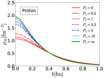
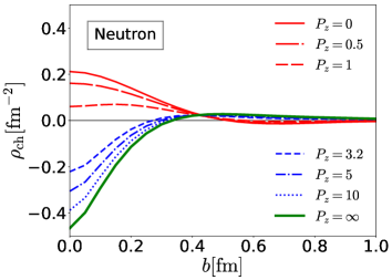
Figure 1: The left (right) panel depicts the transverse charge distributions of the unpolarized proton (neutron) with $P_{z}$ varied from zero to infinity. The EM form factors of both the proton and neutron are taken from the parametrizations given in Ref. Bradford:2006yz .

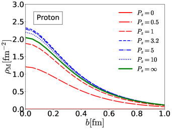
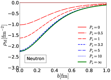
Figure 2: The left (right) panel depicts the transverse magnetization distributions of the unpolarized proton (neutron) with $P_{z}$ varied from zero to infinity. The EM form factors of both the proton and neutron are taken from the parametrizations given in Ref. Bradford:2006yz .

We are now in a position to present and discuss the numerical results of the charge distributions of the unpolarized and transversely polarized nucleons. To derive them, we employ the empirical EM form factors of the nucleon extracted from the experimental data Bradford:2006yz . We first show how the charge distribution of the unpolarized proton undergoes changes as $P_{z}$ increases, which has already been studied in Ref. Lorce:2020onh . For completeness, we present the corresponding results in Fig. 1. As explained in Ref. Lorce:2020onh in detail, the core part of the charge distribution of the proton gets larger as $P_{z}$ increases from $P_{z}=0$ to $P_{z}=\infty$ monotonically whereas the tail part slowly gets lessened. As for the neutron, the core part decreases and turns negative as $P_{z}$ increases, while the tail part gets strengthened and turns positive. This explains the apparent difference between the transverse charge distribution of the neutron in the IMF and the 3D one Miller:2007uy ; Miller:2010nz . In Fig. 2, we show how the magnetization distributions of the proton and neutron undergo changes as $P_{z}$ increases. The general behavior of the magnetization distributions seems to be similar to that of the charge ones. However, as we can see from the left panel of Fig. 2, the magnetization distribution of the proton is maximized at $P_{z}\approx 3.2$ GeV, not at $P_{z}=\infty$. It can be originated from the kinematical factors in Eq. (13). So, this effect is not dynamical but kinematical as shown from Eqs. (11) and (13).

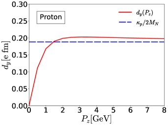
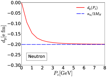
Figure 3: The left (right) panel depicts the induced electric dipole moment of the proton (neutron) as a function of $P_{z}$. The dashed blue line draws the value of the induced electric dipole moment of the nucleon in the IMF.

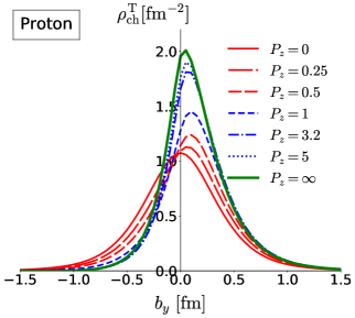
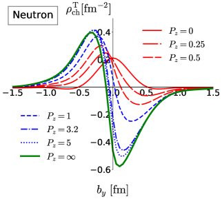
Figure 4: The left (right) panel depicts the transverse charge distributions of the transversely polarized proton (neutron) along the $b_{x}$-direction, with $P_{z}$ varied from zero to infinity. The EM form factors of both the proton and neutron are taken from the parametrizations given in Ref. Bradford:2006yz .

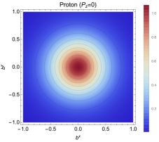
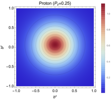
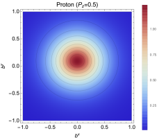
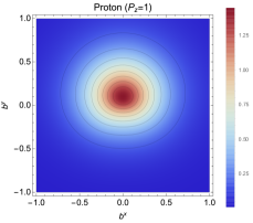
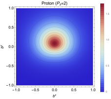
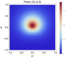
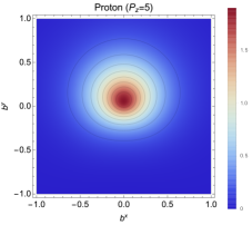
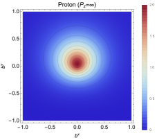
Figure 5: The transverse charge distributions of the transversely polarized proton along the $b_{x}$-direction are illustrated in the 2D transverse plane with $P_{z}$ varied from zero to infinity.

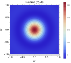
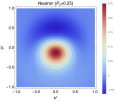
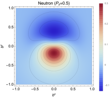
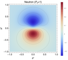
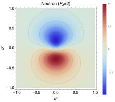
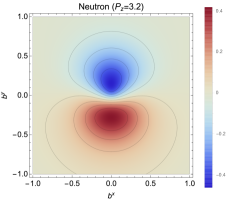
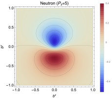
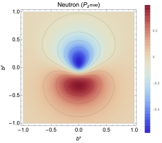
Figure 6: The transverse charge distributions of the transversely polarized neutron along the $b_{x}$-direction are illustrated in the 2D transverse plane with $P_{z}$ varied from zero to infinity.

When the nucleon is transversely polarized along the $b_{x}$-axis, its charge distribution starts to get deformed as $P_{z}$ increases. The external magnetic field is exerted on the moving nucleon, the induced electric dipole moment, which is defined in Eq. (21), brings about the induced electric field $\bm{E}^{\prime}=\gamma(\bm{v}\times\bm{B})$, where $\bm{v}$ is the velocity of the moving nucleon in the EF. The solid curve in the left panel of Fig. 3 draws the magnitude of the nucleon induced electric dipole moment as a function of $P_{z}$. The dashed line depicts the value of $d_{y}$ in the IMF, which is identical to the proton anomalous magnetic moment divided by $2M_{N}$, i.e., $\kappa_{p}/2M_{N}=0.188$ fm. As expected, $d_{y}$ starts to increase as $P_{z}$ increases. Interestingly, however, $d_{z}$ reaches its maximum value at around $P_{z}$ and then diminishes gadually. As $P_{z}\to\infty$, it converges on the dashed line. On the other hand, $d_{y}$ of the neutron becomes negative and its magnitude grows monotonically as $P_{z}$ increases as illustrated in the right panel of Fig. 3. It also converges on $\kappa_{n}/2M_{N}=-0.201$ fm.

The finite value of $d_{y}$ gives rise to the displacement of the charge distribution of the transversely polarized nucleon as shown in Fig. 1 . As $P_{z}$ increases, the left panel of Fig. 4 shows how the charge distribution $\rho_{\mathrm{ch}}^{T}(b,P_{z})$ of the transversely polarized proton is distorted. When the proton starts to move, $\rho_{\mathrm{ch}}^{T}(b,P_{z})$ of the proton begins to get displaced to the positive $b_{y}$-direction. When $P_{z}$ reaches $3.2\,\mathrm{GeV}$, the proton charge distribution is maximally displaced and when it reaches infinity the displacement of the distribution is slightly weakened. When it comes to the neutron case, the situation is more interesting. As shown in the right panel of Fig. 4, the charge distribution of the transversely polarized neutron starts to get deformed in a quite asymmetric way, as $P_{z}$ increases. The results indicate that the down quarks are displaced to the positive $b_{y}$-direction whereas the up quark is shifted to the negative side. In Figs. 5 and 6, we illustrate respectively the 2D transverse charge distributions of the transversely polarized proton and neutron,varying $P_{z}$ from zero to infinity. Figure 5 shows explicitly how the proton charge distribution $\rho_{\mathrm{ch}}^{T}(b,P_{z})$ is distorted as $P_{z}$ increases. We observe that $\rho_{\mathrm{ch}}^{T}(b,P_{z})$ is displaced along the positive $b_{y}$-direction, which is caused by the induced electric dipole field. On the other hand, $\rho_{\mathrm{ch}}^{T}(b,P_{z})$ of the neutron is deformed in a more prominent way. When the neutron is at rest, its transverse charge distribution is shaped in a symmetric form. When it starts to move, the positive charges move to the negative $b_{y}$-direction whereas the negative ones get displaced along the positive $b_{y}$. This is due to the negative values of the electric dipole moment.

III Abel transformation between the 3D Breit and 2D Drell-Yan frames

Recently, Ref. Panteleeva:2021iip showed that the 2D light-front force distributions can be expressed in terms of the 3D BF pressure and shear-force distributions, utilizing the Abel transformation. This indicates that the Abel transformation can map the 3D BF distributions onto the 2D ones in the IMF and they can be reconstructed from the 2D ones by the inverse Abel transform. So, the 3D distributions can still provide intuitive information on the nucleon, though they can only be interpreted as quasi-probabilistic ones. We now want to show how the Abel transformations can be also used to map the 3D charge distributions onto the 2D transverse ones in the IMF.

III.1 Formalism

In the Wigner sense, the Breit frame can be viewed as the rest frame ($\bm{P}=\bm{0}$) of the nucleon localized around $\bm{R}$. The charge ($J^{0}$) and magnetic $(\nabla\times\bm{M})$ quasi-probabilistic distributions are given as the Fourier transforms of the Sachs electric and magnetic form factors, respectively:

$$\rho^{\mathrm{BF}}_{\mathrm{ch}}(r)=\int\frac{d^{3}\Delta}{(2\pi)^{3}}e^{-i\bm{x}\cdot\bm{\Delta}}\frac{m}{P^{0}}G_{E}(t),\ \ \ \rho^{\mathrm{BF}}_{\mathrm{M}}(r)=\int\frac{d^{3}\Delta}{(2\pi)^{3}}e^{-i\bm{x}\cdot\bm{\Delta}}\frac{m}{P^{0}}G_{M}(t),$$ (22)

which are the fully relativistic expressions Lorce:2020onh . If we take the nonrelativistic limit, i.e.,  ${m}/{P^{0}}\sim 1$, we arrive at the expressions

$$\rho^{\mathrm{NR}}_{\mathrm{ch}}(r)=\int\frac{d^{3}\Delta}{(2\pi)^{3}}e^{-i\bm{x}\cdot\bm{\Delta}}G_{E}(t),\ \ \ \rho^{\mathrm{NR}}_{\mathrm{M}}(r)=\int\frac{d^{3}\Delta}{(2\pi)^{3}}e^{-i\bm{x}\cdot\bm{\Delta}}G_{M}(t),$$ (23)

which can be often found in textbooks. However, the definitions of the charge and magnetization distributions given in Eq. (23) have been criticized over decades Yennie:1957 ; Burkardt:2000za ; Burkardt:2002hr ; Miller:2007uy ; Miller:2010nz ; Jaffe:2020ebz ; Lorce:2020onh . As mentioned already, the main criticism comes from the fact that the size of the nucleon is comparable to its Compton wavelength, which implies that the nucleon is a relativistic particle. So, we are not able to construct the wavepacket for the nucleon, which can be localized within the space characterized by the Compton wavelength. Thus, the charge distribution defined in Eq. (23) cannot be interpreted as the quantum-mechanical probabilistic one. To define the charge distribution correctly as a quantum-mechanical probabilistic one, one should introduce the corresponding one in the transverse plane to the direction of the moving nucleon with the infinite longitudinal momentum Burkardt:2000za ; Burkardt:2002hr ; Miller:2007uy ; Miller:2010nz . While this low-dimensional transverse charge distribution is considered as a price one should pay to define it as a quantum-mechanically meaningful one, it rather paves the way to understand the internal structure of the nucleon in a more profound way. Various transverse distributions, which correspond to the EM, gravitational and tensor form factors, reveal unprecedented features of the nucleon. In this sense, the Abel and Radon transformations also provide a new way of examining the structure of the nucleon.

As mentioned in the previous section, the transverse charge and magnetization densities are obtained respectively by the Fourier transforms of the Dirac and Pauli form factors

$$\rho_{\mathrm{ch}}(b)=\int\frac{d^{2}\bm{\Delta}}{(2\pi)^{2}}e^{-i\bm{b}\cdot\bm{\Delta}}F_{1}(t),\ \ \ \rho_{\mathrm{M}}(b)=\int\frac{d^{2}\bm{\Delta}}{(2\pi)^{2}}e^{-i\bm{b}\cdot\bm{\Delta}}F_{2}(t).$$ (24)

Employing now the Abel transform Abel ; Natterer:2001 for a spherically symmetric particle such as the nucleon, we can map the 3D charge and magnetization distributions onto the transverse charge and magnetization distributions. In fact, the Abel transformation was already applied to the deeply virtual Compton scattering Polyakov:2007rv ; Moiseeva:2008qd and the energy-momentum tensor distributions Panteleeva:2021iip ; Kim:2021jjf . The Able transform and its inverse transform are defined as

$$A[g](b)=\mathcal{G}(b)=\int^{\infty}_{b}\frac{dr}{r}\frac{g(r)}{\sqrt{r^{2}-b^{2}}},\ \ \ g(r)=-\frac{2}{\pi}r^{2}\int^{\infty}_{r}db\frac{d\mathcal{G}(b)}{db}\frac{g(r)}{\sqrt{b^{2}-r^{2}}}.$$ (25)

Thus, $A[g](b):=\mathcal{G}(b)$ is called the Abel image of the function $g(r)$. In addition, a useful relation for the Mellin moments of the Abel images can be obtained as Panteleeva:2021iip :

$$\int^{\infty}_{0}b^{N}A[g](b)\,db=\frac{\sqrt{\pi}}{2}\frac{\Gamma\left(\frac{N+1}{2}\right)}{\Gamma\left(\frac{N+2}{2}\right)}\int^{\infty}_{0}\,r^{N-1}g(r)dr.$$ (26)

The relation (26) is valid as far as the 3D EM distributions in the distance decrease faster than any order of $r^{N-1}$. The 2D distribution in the IMF can be easily connected to the 3D distribution in the BF

$$\rho_{\mathrm{ch}}(b)+\frac{1}{4M_{N}^{2}}\partial_{\perp}^{2}\rho_{\mathrm{M}}(b)=\int^{\infty}_{b}\frac{2r\,dr}{\sqrt{r^{2}-b^{2}}}\rho^{\mathrm{NR}}_{\mathrm{ch}}(r),\ \ \rho_{\mathrm{ch}}(b)+\rho_{M}(b)=\int^{\infty}_{b}\frac{2r\,dr}{\sqrt{r^{2}-b^{2}}}\rho^{\mathrm{NR}}_{\mathrm{M}}(r),$$ (27)

which are just the Abel transforms of the 3D charge and magnetization distributions . It is of great importance to observe that when the Abel transforms of the 3D BF charge and magnetization distributions yield naturally the combination of the transverse charge and magnetization ones, which are the consequence of the Lorentz boost. In fact, it is one of the essential features of the Abel transform that it properly incorporates the effects of the Lorentz boost.

Making use of Eq. (25), the Abel images of the 3D charge and magnetic distributions in the BF are expressed by

$$A[2r^{2}\rho^{\mathrm{NR}}_{\mathrm{M}}](b)=\rho_{\mathrm{ch}}(b)+\rho_{M}(b),\;\;\;A[2r^{2}\rho^{\mathrm{NR}}_{\mathrm{ch}}(r)](b)=\rho_{\mathrm{ch}}(b)+\frac{1}{4M_{N}^{2}}\partial_{\perp}^{2}\rho_{M}(b),$$ (28)

which are identical to the 2D transverse charge and magnetization distributions. Note, however, that it is difficult to express the 3D distributions together with the relativistic corrections $\sim 1/P^{0}$ in the BF in terms of the 2D transverse distributions in the IMF due to the non-locality of the kinematical factor $P^{0}$. It is also interesting to examine the Mellin moment of the Abel image. For $N=1$, one has an equality of the charge and magnetic moments in both the 2D and 3D frames. For $N=3$, one arrives at

$$Q\langle r^{2}\rangle_{\mathrm{ch}}=\frac{3}{2}\left(Q\langle b^{2}\rangle_{\mathrm{ch}}+\frac{\kappa_{N}}{M_{N}^{2}}\right),\;\;\;\langle r^{2}\rangle_{M}=\frac{3}{2}\frac{\langle b^{2}\rangle_{\mathrm{ch}}Q+\langle b^{2}\rangle_{M}\kappa_{N}}{Q+\kappa_{N}},$$ (29)

where $Q$ represents the charge of the nucleon and $\kappa_{N}$ is the corresponding anomalous magnetic moment.

III.2 Results and discussion

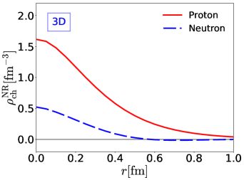
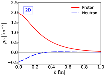
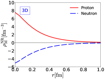
Figure 7: The 3D (transverse) charge and magnetization distributions are presented in the BF (IMF) in the left (right) upper and lower panels, respectively. The solid and dashed curves denote the cases of the proton and neutron, respectively. The charge distributions are normalized to be its charge whereas the 3D (2D) magnetization distribution is normalized to be the corresponding magnetic dipole moments $\mu_{p}$ and $\mu_{n}$ in units of the nuclear magneton (anomalous magnetic moment $\kappa_{N}$).

The upper panel of Figure 7 draws the 3D charge distributions in the BF (left panel) and the transverse charge distributions in the IMF (right panel). As anticipated, both the transverse charge distributions of the proton and neutron are properly obtained from the 3D ones by the Abel transformation. The results for the 2D transverse charge distributions are identical to those obtained in Fig. 1 when $P_{z}\to\infty$. In particular, it is remarkable to see that the transverse charge distributions of the neutron in the IMF are correctly reproduced. As already found in Eq. (27), As $P_{z}\to\infty$, the effect of the magnetization enters into the transverse charge distribution, which makes core part of the neutron turn negative. Thus, the Abel transformation maps correctly the 3D charge distributions of the nucleon at rest onto the 2D transverse ones in the IMF.

As shown in the lower panel of Fig. 7, both the transverse magnetization distributions of the proton and neutron are also derived correctly, which have also shown in Fig. 2. The present results draw two important physical implications: Firstly, the Abel transformation can also be applied to the charge and magnetization distributions of the nucleon. Secondly, while the 3D charge distributions have only the quasi-probabilistic meaning in the Wigner sense, they still give us valuable insight into understanding the internal structure of the nucleon with the help of the Abel transformations.

IV Summary and conclusions 

In the present work, we aimed at investigating how the transverse charge and magnetization distributions of both the unpolarized and transversely polarized nucleon get displaced as its longitudinal momentum increases from zero to infinity. Interestingly, the transverse magnetization distribution of the nucleon is maximized not at the infinite momentum but at around 3.2 GeV. This originates from the kinematical reason. When the nucleon is transversely polarized along the positive $x$-direction of the impact parameter, the induced electric dipole moment is produced at the finite value of the longitudinal momentum. This causes the displacement of the transverse charge distribution of the proton along the positive $y$-direction. On the other hand, that of the neutron shows more interesting behavior. The positive charges, which represent the up valence quark inside a neutron, are displaced to the negative direction whereas the negative charges or the down valence quarks are moved toward the positive direction. This is due to the negative values of the electric dipole moment of the neutron.

In the second part of the present work, we examined how the Abel transformations map the 3D charge distributions in the Breit frame on to the 2D transverse ones in the Drell-Yan frame or the infinite momentum frame. As expected, the Abel transformations successfully project the 3D BF charge distributions onto the 2D transverse plane in the Drell-Yan frame. Both the 3D charge and magnetization distributions in the Breit frame are expressed in terms of the transverse charge and magnetization ones in the Drell-Yan frame. Keep in mind that the Lorentz boost makes the charge and magnetization distributions mixed, the Abel transformations respect the Lorentz boost, so that we have properly reproduced the transverse charge distributions in the Drell-Yan frame. We found the physical implications of the Abel transformation in the present work: The Abel transformation indeed connects the 3D charge and magnetization distributions to the 2D transverse ones, which implies that the 3D distributions can still provide insight into the internal structure of the nucleon, even though they have only the quasi-probabilistic meaning.

When we consider the interpolation between the 3D distributions and 2D transverse ones for particles with spin higher than 1/2, one has to employ the Radon transformation instead of the Abel one, as already proposed in Panteleeva:2021iip . The corresponding investigation is under way.

- (1) R. Hofstadter, Rev. Mod. Phys. 28, 214 (1956).
- (2) V. Punjabi, C. F. Perdrisat, M. K. Jones, E. J. Brash and C. E. Carlson, Eur. Phys. J. A 51, 79 (2015).
- (3) F. J. Ernst, R. G. Sachs and K. C. Wali, Phys. Rev. 119, 1105 (1960).
- (4) R. G. Sachs, Phys. Rev. 126, 2256 (1962).
- (5) D.R. Yennie, M.M. Levy, D.G. Ravenhall, Rev. Mod .Phys. 29, 144 (1957).
- (6) M. Burkardt, Phys. Rev. D 62, 071503 (2000) Erratum: [Phys. Rev. D 66, 119903 (2002)].
- (7) M. Burkardt, Int. J. Mod. Phys. A 18, 173 (2003).
- (8) G. A. Miller, Phys. Rev. Lett. 99, 112001 (2007).
- (9) G. A. Miller, Ann. Rev. Nucl. Part. Sci. 60, 1 (2010).
- (10) C. Lorcé, Phys. Rev. Lett. 125 (2020) 232002.
- (11) R. L. Jaffe, Phys. Rev. D 103, 016017 (2021).
- (12) E. P. Wigner, Phys. Rev. 40, 749 (1932).
- (13) M. Hillery, R. F. O’Connell, M. O. Scully and E. P. Wigner, Phys. Rept. 1060, 121 (1984).
- (14) H.-W. Lee, Phys. Rept. 259, 147 (1995).
- (15) D. Müller, D. Robaschik, B. Geyer, F.-M. Dittes and J. Hořejši, Fortsch. Phys. 42, 101 (1994).
- (16) X. D. Ji, Phys. Rev. D 55, 7114 (1997).
- (17) A. V. Radyushkin, Phys. Rev. D 56, 5524 (1997).
- (18) K. Goeke, M. V. Polyakov and M. Vanderhaeghen, Prog. Part. Nucl. Phys. 47, 401 (2001).
- (19) M. Diehl, Phys. Rept. 388, 41 (2003).
- (20) X. Ji, Ann. Rev. Nucl. Part. Sci. 54, 413 (2004).
- (21) A. V. Belitsky and A. V. Radyushkin, Phys. Rept. 418, 1 (2005).
- (22) C. Lorcé, L. Mantovani and B. Pasquini, Phys. Lett. B 776, 38 (2018).
- (23) C. Lorcé, Eur. Phys. J. C 78, 785 (2018).
- (24) C. Lorcé, H. Moutarde and A. P. Trawiński, Eur. Phys. J. C 79, 89 (2019).
- (25) C. Lorcé, Eur. Phys. J. C 81, 413 (2021).
- (26) J. Y. Panteleeva and M. V. Polyakov, arXiv:2102.10902 [hep-ph].
- (27) N.H. Abel, J. Reine und Angew. Math. 1, 153 (1826).
- (28) U. Leonhardt, “Measuring the quantum state of light, Cambridge Studies in Modern Optics”, (Cambridge University Press, Cambridge, 1997).
- (29) F. Natterer, “The Mathematics of Computerized Tomography”, (John Wiley & Sons, New York, 2001).
- (30) M. V. Polyakov, Phys. Lett. B 659, 542 (2008).
- (31) A. M. Moiseeva and M. V. Polyakov, Nucl. Phys. B 832, 241 (2010).
- (32) J. Y. Kim and H.-Ch. Kim, [arXiv:2105.10279 [hep-ph]].
- (33) J. Radon, Berichte über die Verhandlungen der Köiglich-Sächsischen Gesellschaft der Wissenschaften zu Leipzig, Mathematisch-Physische Klasse 69, 262 (1917).
- (34) C. E. Carlson and M. Vanderhaeghen, Phys. Rev. Lett. 100, 032004 (2008).
- (35) R. Bradford, A. Bodek, H. S. Budd and J. Arrington, Nucl. Phys. B Proc. Suppl. 159, 127 (2006).