Identification of the cosmogenic ¹¹C background in large volumes of liquid scintillators with Borexino

Résumé

Cosmogenic radio-nuclei are an important source of background for low-energy neutrino experiments. In Borexino, cosmogenic ¹¹C decays outnumber solar $pep$ and CNO neutrino events by about ten to one. In order to extract the flux of these two neutrino species, a highly efficient identification of this background is mandatory. We present here the details of the most consolidated strategy, used throughout Borexino solar neutrino measurements. It hinges upon finding the space-time correlations between ¹¹C decays, the preceding parent muons and the accompanying neutrons. This article describes the working principles and evaluates the performance of this Three-Fold Coincidence (TFC) technique in its two current implementations: a hard-cut and a likelihood-based approach. Both show stable performances throughout Borexino Phases II (2012-2016) and III (2016-2020) data sets, with a ¹¹C tagging efficiency of $\sim$90 % and $\sim$63-66 % of the exposure surviving the tagging. We present also a novel technique that targets specifically ¹¹C produced in high-multiplicity during major spallation events. Such ¹¹C appear as a burst of events, whose space-time correlation can be exploited. Burst identification can be combined with the TFC to obtain about the same tagging efficiency of $\sim$90% but with a higher fraction of the exposure surviving, in the range of $\sim$66-68 %.

1 Introduction

Since 2007, the Borexino detector has been observing solar neutrinos from the depths of the Gran Sasso National Laboratory (Italy). Designed for the spectroscopy of low energy neutrinos detected via elastic scattering off electrons, Borexino has accomplished individual measurements of the solar ⁷Be bx_7Be , ⁸B bx_8B , $pep$ bx_pep , and $pp$ neutrino fluxes bx_pp . Moreover, Borexino has performed a comprehensive spectroscopic measurement of the entire neutrino spectrum emitted in the $pp$-chain bx_nature ; bx_nusol ; bx_8B_new . Most recently, Borexino achieved the first direct observation of neutrinos produced in the solar CNO cycle bx_cno ; bx_cno_sens .

While there are several elements that contributed to the success of Borexino, we focus here on the analysis strategy that has been developed for the identification of cosmogenic background in the 1–2 MeV spectral region (originally proposed in tfc_deutsch ). The observation of $pep$ and CNO neutrinos is made possible by the suppression of the $\beta^{+}$-decays of ¹¹C that are otherwise largely indistinguishable from neutrino-induced electron recoils on an event-by-event basis. In organic scintillators, ¹¹C is being produced by cosmic muons that penetrate the rock coverage of the laboratory and induce spallation processes on carbon of type $\mu+^{12}\text{C}\rightarrow\mu+^{11}\text{C}+n$. A discussion of the processes that contribute to ¹¹C isotope production can be found in c11prod . The isotope features a lifetime of 29.4 minutes and a $Q$-value of 0.96 MeV. Due to positron annihilation, the visible spectrum is shifted to higher energies, covering a range between $\sim$0.8 and $\sim$2 MeV.

Figure 1 shows the main neutrino signal and radioactive background contributions to the visible energy spectrum of Borexino. At first glance, detection of $pep$ and CNO neutrinos seems not very promising since other solar neutrino species cover the lower part of their spectra while towards the upper end ¹¹C overtops their signals by about an order of magnitude. An efficient veto strategy for ¹¹C is a necessary prerequisite for overcoming this disadvantageous situation.

The present article illustrates two analysis techniques for an effective ¹¹C suppression. The first is the Three-Fold Coincidence (TFC) technique. The TFC is formed by the space and time correlation of ¹¹C events with their parent muons and the neutrons that in most cases accompany ¹¹C production. By now, the technique has been extensively used in Borexino analyses. TFC creates two subsets of data: (1) a ¹¹C-depleted set that is including over 60% of the exposure but less than 10% of the ¹¹C events; (2) a ¹¹C-enriched set with the complementary exposure and ¹¹C events. Both datasets are used in the multivariate fit that leads to the extraction of the solar neutrino signals as explained in bx_long ; bx_nusol .

The second technique is the Burst Identification (BI) technique, a new tagging strategy that targets ¹¹C events originating from a single hadronic shower upon the passage of a muon. These events are visible in bursts and are space-time correlated among themselves: due to the negligible convective motion of the scintillator in the timescale of the ¹¹C mean life, they remain essentially aligned along the parent muon track. Since the BI technique on its own does not provide sufficient tagging efficiency for solar neutrino analyses, it is only used in combination with the TFC in Borexino. However, the BI method might be interesting as a stand-alone solution for experimental setups that do not provide sufficient information for a TFC-like approach.

In this article, we first recall the key features of the Borexino detector (Section 2); we then review the TFC technique, presenting the two most developed implementations that use either a cut-based or likelihood-based approach and their comparative performances (Section 3); we go on to discuss the new BI technique and the gain in ¹¹C-depleted exposure that can result from a combined application of TFC and BI (Section 4), before presenting our conclusions in Section 5.

It is worth to note that both the TFC and the BI algorithms have been developed for the tagging of ¹¹C but are not limited to this specific cosmogenic isotope. Despite some variability in the underlying production processes kamland_cosmogenics , the creation of radioactive isotopes in organic scintillator is closely linked to muons inducing hadronic showers, resulting in especially bright muon events and subsequent bursts of delayed neutron captures. Both tagging techniques are of immediate use for upcoming neutrino detectors based on organic scintillators snoplus ; juno but may as well be of interest for water Cherenkov detectors with neutron-tagging capabilities gadzooks ; HK ; SK_tagging or hybrid detectors theia .

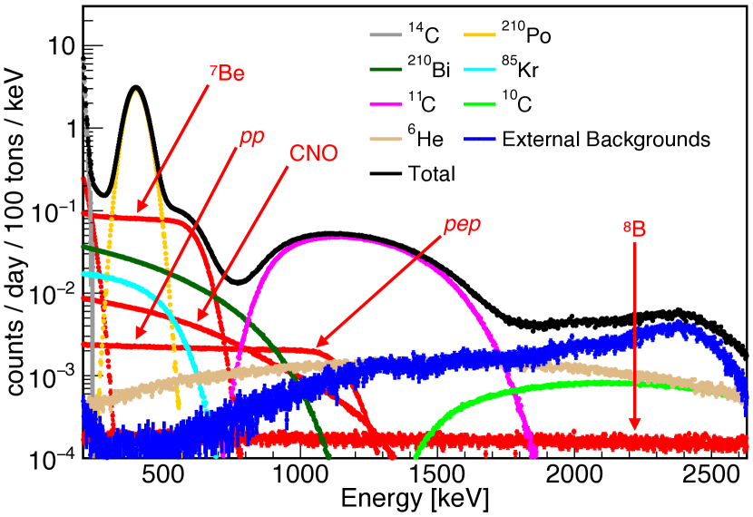
Figure 1: Expected spectrum in Borexino from Monte Carlo simulations. Electron recoil energy due to neutrino interactions (red lines) and background components (other colors). The Fiducial Volume applied is described in Section 2.

2 The Borexino detector

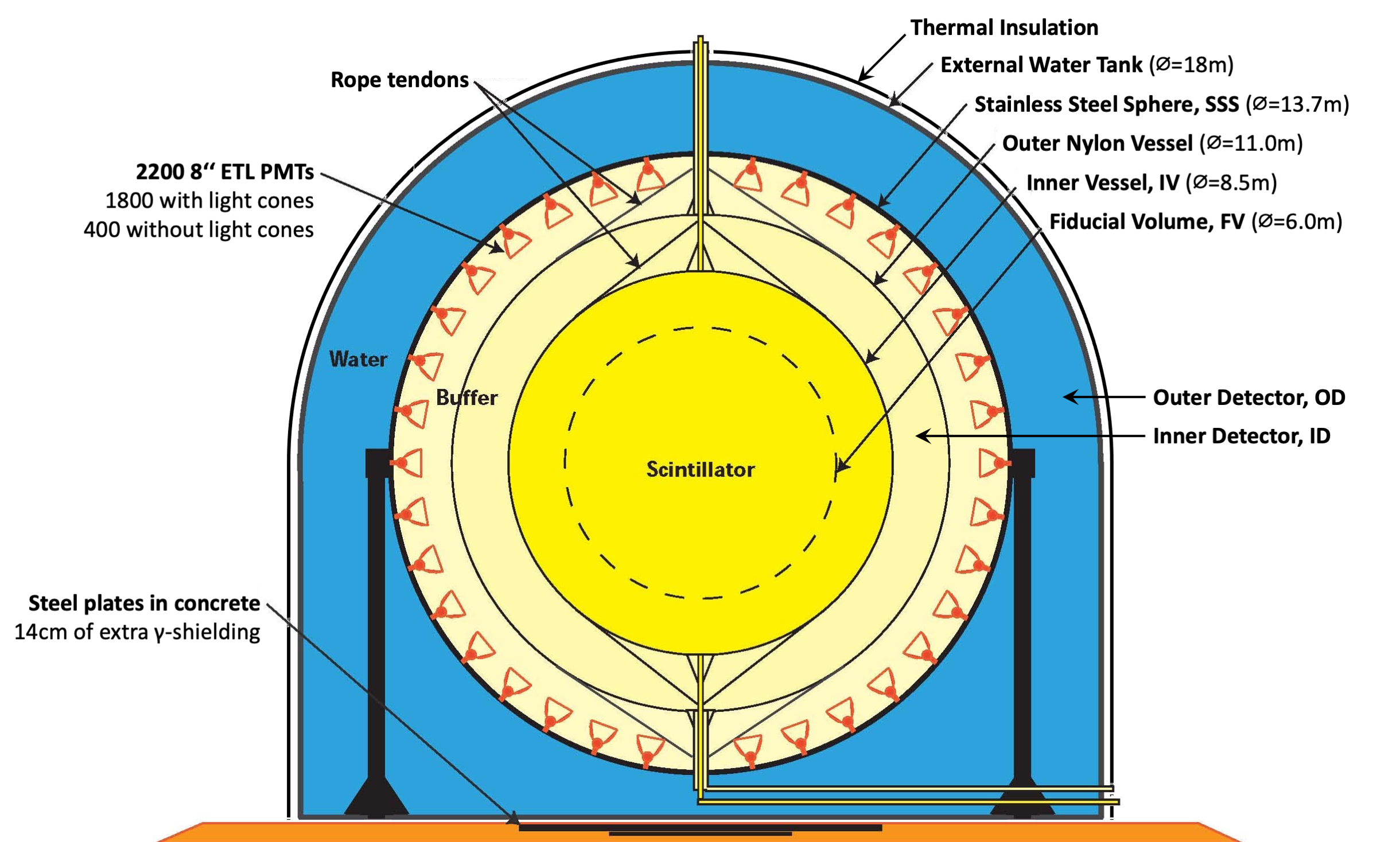
Figure 2: Sketch of the Borexino Detector.

A schematic drawing of the Borexino detector bx_detector is shown in Figure 2. The neutrino target consists of 278 t of organic scintillator composed of the solvent PC (1,2,4-trimethylbenzene) doped with the wavelength shifter PPO (2,5-diphenyloxazole) at a concentration of 1.5 g/l. The scintillator mixture is contained in a spherical and transparent nylon Inner Vessel (IV) with a diameter of 8.5 m and a thickness of 125 $\upmu$m. To shield this central target from external $\gamma$-ray backgrounds and to absorb emanating radon, the IV is surrounded by two layers of buffer liquid in which the light quencher DMP (dimethylphthalate) is added to the scintillator solvent. A Stainless Steel Sphere (SSS) of 13.7 m diameter holding 2212 8” photomultiplier tubes (PMTs) completes the Inner Detector (ID). PMTs are inward-facing and detect the scintillation light caused by particle interactions in the central region. The ID is embedded in a steel dome of 18 m diameter and 16.9 m height that is filled with 2.1 kt of ultra-pure water. The outer surface of the SSS and the floor of the water tank are instrumented with additional 208 PMTs. This Outer Detector (OD) provides efficient detection and tracking of cosmic muons via the Cherenkov light that is emitted during their passage through the water. Neutrons created by the passage of muons are quickly thermalized and captured on hydrogen (carbon in 1% of the cases) in the scintillator after $\tau_{n}\sim 260\,\upmu$s bx_cosmogenics with the emission of a 2.2 MeV (4.9 MeV) de-excitation gamma-ray. Muon and neutron detection in Borexino is described in detail in bx_od . A thorough analysis of all cosmogenic backgrounds can be found in bx_cosmogenics and the most recent update on the cosmic muons and neutrons in bx_muon_seasonal .

Event reconstruction.

In Borexino, a physical event is defined by the firing of several PMTs of the ID within a short period of time (typically 20–25 PMTs in 60–100 ns, changing over time). This occurrence causes a trigger signal and opens an acquisition window of 16 $\upmu$s during which all PMT pulses are saved. As this window may contain more than one physical event, an offline clustering algorithm identifies pulses within a short time window (several 100 ns) as belonging to a specific event. Since the scintillation light output is proportional to the deposited energy, the number of pulses (“hit”) recorded by the PMTs for a given cluster, $N_{\text{hits}}$, is used as energy estimator. We record about 500 photoelectrons per MeV of deposited energy. In order to account for the increasing number of malfunctioning PMTs throughout the data set bx_nusol , the number of hits is always normalized to 2000 live channels. The position of the scintillation events in the scintillator volume is reconstructed based on the time-of-flight of the scintillation photons from vertex to PMTs. The reconstruction algorithm uses PDFs for the expected arrival time distributions at the PMTs to take into account both propagation effects and the time profile of the scintillation process bx_long .

Muon and Neutron Windows.

A muon crossing the scintillator target is expected to cause sizable signals in both ID and OD. As for ordinary events, the ID trigger opens a 16 $\upmu$s-long “Main Window” (MW) for which all hits are saved. The OD issues an additional trigger flag with high efficiency. In case of its presence, the MW is followed by a substantially longer “Neutron Window” (NW): 1.6 ms. This is meant to catch the subsequent signals due to the capture of muon-induced neutrons without requiring explicit triggers. Given the value of $\tau_{n}$, about 6% of neutrons are collected in the MW and the rest in the NW.

Empty Boards condition.

The ID is designed for low energy spectroscopy, so scintillator-crossing muons that generate a huge amount of light have a significant chance of saturating the electronics memory. Consequently, the reconstruction of the energy and of the position of the neutron-capture gammas following such event can be troublesome. Effects are more severe in the MW than in the NW. It has been found that this condition can be quantified by the number of electronic boards that show no data for MW and NW in any of their eight channels when memory saturation occurs. Thus, the number of boards devoid of hits (out of a total of 280 boards) is counted and stored for analysis as parameter $N_{\text{EB}}$ (# of Empty Boards).

Neutron identification.

Luminous muon events produce a long tail of trailing hits that extend into the NW (e.g. by after pulsing of PMTs). A specifically adapted clustering algorithm has been developed for both the muon MW and NW to find physical events superimposed to this background. This task is further complicated be the aforementioned presence of saturation effects.

Due to its considerable length the NW contains not only neutrons (and cosmogenic isotopes) but for the most part accidental counts. These are dominated by low energy ¹⁴C decays that occur at a rate of about 100 s^-1 bx_pp . To avoid mis-counting those and other low-energy events as neutron captures, an energy selection threshold has been introduced at $N_{\text{thr}}=385$ hits (corresponding roughly to 770 keV). To take into account the saturation effects that diminish the number of hits collected from a neutron event, the selection criterium is adjusted to $N_{\text{hits}}>N_{\text{thr}}-2\times N_{\text{EB}}$.

Neutron vertex reconstruction.

Following bright muons, the accuracy of vertex reconstruction can be severely affected by electronics saturation effects. Therefore, position reconstruction is ineffective for neutrons in the MW and can still be severely affected in the NW. The TFC algorithms described below take this into account by introducing Full Volume Vetoes (see Section 3.3) in presence of severe saturation effects. The BI algorithm described in Section 4 can be used as an alternative, more effective way to target ¹¹C produced under these circumstances.

Fiducial volume.

Unless otherwise noted, in this paper we refer to fiducial volume as to the one used in the $pp$-chain bx_nature and in the CNO bx_cno neutrino analyses. This means considering events with a reconstructed position within a 2.8 m radius from the center of the detector and vertical coordinate in the range [-1.8, 2.2] m.

Data taking campaigns.

The Borexino data used throughout this paper refer to Phase-II and Phase-III of the data taking campaign, ranging respectively from 14 December 2011 till 21 May 2016 and from 17 July 2016 till 1 March 2020. The average number of working PMTs during Phase-II and III was about 1500 and about 1200, respectively.

A temperature control strategy was gradually adopted throughout Phase-III to prevent convection in the liquid scintillator bx_cno in order to stabilize internal radioactive background levels. However we note that no impact is expected in ¹¹C suppression mechanisms as the observed convective time scale is much longer than ¹¹C mean life.

3 Three-Fold Coincidence

The TFC identifies ¹¹C candidates by their space and time correlation with the preceding parent muons and muon-induced neutrons and splits the original data sample into two sub-samples: one containing the ¹¹C-tagged events (enriched sample) and another one where most ¹¹C events are removed (depleted sample).

In practice, the procedure is complicated by the relatively long lifetime of the ¹¹C isotope ($\tau_{{}^{11}{\rm C}}=29.4$ min) compared to the rate of muons crossing the Borexino ID (3 min^-1). While the association of muon tracks and subsequent neutron capture vertices ($\tau_{n}\sim 260\,\upmu$s) is straight-forward, tagging conditions have to be maintained for several $\tau_{{}^{11}{\rm C}}$ and thus select not only ¹¹C candidates but also substantial amounts of non-cosmogenic events. While we refer to the latter as neutrino events in the following, it is worth to point out that this event category contains as well a large amount of decays caused by internal and external radioactivity that we include under this denomination for the sake of simplicity.

Typically, about 40 % of the exposure is contained in the ¹¹C-enriched data set that includes over 90% of ¹¹C decays. The complementary ¹¹C-depleted data set thus mostly consists of neutrino events and corresponds to $\sim$60 % of the exposure. This latter set is the most relevant for $pep$ and CNO neutrino analyses. Thus, the goal of the TFC algorithms is to minimize the ¹¹C that remains in the ¹¹C-depleted subset and to maximize the fraction of the exposure that contributes to it.

We note that in c11prod it is theoretically calculated that about 5% of the ¹¹C production does not have a neutron associated. Although in principle this could imply an inefficiency of the TFC method, several ¹¹C atoms and additional neutrons are generally produced by the same parent muon, effectively limiting the impact of these invisible channels.

This section describes the two TFC approaches used in Borexino analyses: the Hard Cut approach (HC-TFC, Section 3.1) and the Likelihood approach (LH-TFC, Section 3.2).

HC-TFC generates a list of space-time veto regions within the exposure upon meeting certain conditions (typically a muon followed by one or more neutrons). All regular events are then tested against the regions in the list and if they fall within one (or more) they are labelled as ¹¹C. LH-TFC builds for each event a likelihood to be a ¹¹C decay based of its space-time distance from preceding muon-neutron pairs and applies the ¹¹C tag if the likelihood exceeds a programmable threshold. ¹¹C-tagged events will include a fraction of falsely tagged neutrino events that are thus included in the ¹¹C-enriched spectrum. Vice versa, the ¹¹C-depleted data set will contain a residual of ¹¹C decays. Their fraction represents the inefficiency of the TFC method.

Figure 3 shows the ¹¹C-depleted and -enriched visible energy spectra based on Borexino Phase-II data. The effect of the TFC in the ¹¹C energy range (0.75–1.87 MeV) is striking. A difference in the spectral shapes persists at even higher energies. This difference can be attributed to other cosmogenic isotopes (predominantly ¹⁰C and ⁶He) that feature higher spectral end-points and that are picked up as well by the TFC tagging.

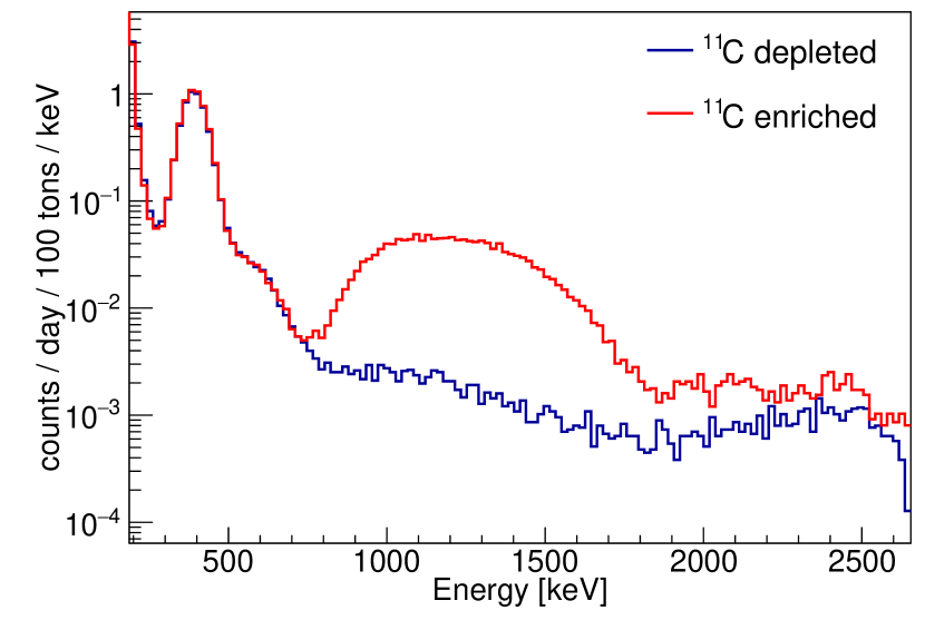
Figure 3: ¹¹C-depleted (blue line) and enriched (red line) charge spectra created with the TFC method for Phase-II. Spectra are normalized to the same exposure. Only basic cuts that remove muon and noise events are applied. The spectral difference above 1800 keV is caused by the TFC tagging of cosmogenic ⁶He and ¹⁰C.

The fraction of exposure that contributes to each spectrum is computed within each TFC algorithm by generating random events with uniform time and position distributions within the fiducial volume, effectively reproducing every real run. These events are then tested against the same list of veto regions or likelihood condition of the real events.

3.1 Hard Cut approach

The first approach for the suppression of the ¹¹C background developed in Borexino bx_long is based on defining a list of space-time veto regions in the dataset. A region is added to the list upon the occurrence of a combination of muon and neutron events. Each region holds for a programmable time after the events that generated it. We set this time to 2.5 h, approximately five times the ¹¹C mean time, based on an optimization for tagging efficiency and exposure (see Section 3.4). Regular events are then checked against the list of regions and if falling within one or more they are flagged as ¹¹C.

We now describe the different conditions that determine the creation of a veto region. In the definition of the regions we use the concept of neutron multiplicity, indicating how many clusters of PMT hits that follow a muon event could possibly be due to a $n$-capture gamma. In the MW we count $n_{\mu n}$ as the number of clusters found by the ad-hoc cluster-finding algorithm that accounts for the underlying tail of the muon event, excluding the first 3.5 $\upmu$s of the window. In the NW we count $n_{n}$ as the number of clusters that meet the requirement expressed in Section 2.

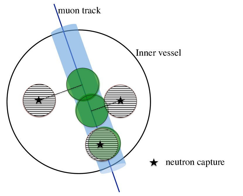
Figure 4: HC-TFC working principle. Upon the passage of a muon through the IV, geometrical veto regions are defined: a cylinder around the muon track (blue), and spheres around the n-capture points (shaded) and around their projection upon the track (green). The typical radius of the cylindrical (spherical) regions is 0.7 m (1.2 m). The picture is not to scale.

Upon finding a muon followed by at least one neutron cluster, we define geometrical veto regions: (1) a cylindrical region around the reconstructed muon track (if available); (2) a spherical region around the $n$-capture reconstructed position in the NW; (3) a spherical region around the projection point of the $n$-capture position in the NW onto the muon track (if available). The working principle is depicted in Figure 4. After tuning for tagging efficiency and exposure (see Section 3.4), the radius of the cylindrical and spherical regions are chosen to be 0.7 m and 1.2 m, respectively as summarized in Figure 4 caption.

Concerning the tracking of muons, as reported in bx_od , Borexino has developed two algorithms based on the ID signals and one based on the Cherenkov light recorded by the OD. The track resulting from a global fit of four entry/exit-points (two from either of the ID-based algorithms and two from the OD-based one) is chosen for the vast majority of muons. In those cases when the fit result is inadequate, we rely on the available results of the individual algorithms bx_od . In the rare cases ($\sim$ 0.1 $\mu$/d) for which none of the tracking algorithms could provide a meaningful track, we apply a Full Volume Veto (introduced in Section 3.3).

In the years up to 2012, the CNGS neutrino beam aimed from CERN to Gran Sasso induced $\nu_{\mu}$ interactions in both the Borexino detector and the rock upstream, creating a sizable amount of muons crossing the scintillator volume bx_cngs . These muons are relatively low in energy ($\sim$ 20 GeV) and, as expected, we observe that they do not significantly contribute to ¹¹C background. Therefore, we exclude them from the potentially veto-triggering muons based on the beam time stamps.

In addition to the veto regions described in this section, HC-TFC also implements the Full Volume Vetoes described in Section 3.3.

3.2 Likelihood approach

The implementation of the TFC described above applies hard cuts between muons, neutrons, and $\beta$-events to make a binary decision whether a candidate event should be regarded as a neutrino or ¹¹C event. In contrast, the approach detailed in this section tries a further optimization of tagging efficiency and dead-time reduction by assigning each event a non-binary likelihood to be cosmogenic. A likelihood ${\cal L}=\prod_{i}p_{i}$ is obtained from the product of several partial probabilities to be ¹¹C, $p_{i}$, that are based on a set of TFC discrimination parameters.

The discrimination parameters are largely the same as for the HC-TFC (Section 3.1), i.e. the spatial distances and time elapsed with regards to the potential parent muons and neutrons. In addition, it permits to directly include the neutron multiplicity, the presence of neutrons within the MW, and the differential energy loss $dE/dx$ of the parent muon. The corresponding probability profiles $p_{i}$ can be obtained directly from data (see below) and are displayed in Figure 6.

The rationale behind this approach is that a ¹¹C candidate closely missing all hard-cut criteria to be cosmogenic would still score high in the likelihood approach, while an event fulfilling only narrowly one selection criterium will not be selected. Thus, the likelihood is expected to do particularly well in those cases. It also permits to balance between spatial and time distance between muons (or neutrons) and ¹¹C candidates, meaning effectively that wider spatial cuts are implemented in case of shorter time differences.

A similar tagging scheme for the cosmogenic isotope ⁹Li has been successfully applied in the Double-Chooz experiment theta13-doublechooz ; Li9-doublechooz .

3.2.1 Data-driven probability profiles

The majority of probability profiles has been derived directly from the data, using the 2012 data set. For a given discrimination parameter $i$, the partial probability $p_{i}$ is determined by sorting the data set into several subsamples based on intervals of the parameter value. In each subsample, the relative contributions of ¹¹C and uncorrelated events is evaluated based on the time difference ($\Delta t_{k}$) profile between a ¹¹C-candidate and all preceding muons $(k)$ in the last two hours. As an example, Figure 5 shows the $\Delta t_{k}$ profile of ¹¹C-candidates selected by the distance from the parent muon track $d_{\mu}$ in the interval $[1.0\,{\rm m};1.2\,{\rm m})$. The $\Delta t_{k}$ distribution contains a flat component associated to accidental coincidences of unrelated $\mu$-candidate pairs as well as an exponentially decaying component (following the ¹¹C lifetime) of true $\mu$-¹¹C coincidences. As shown in Figure 5, the relative fraction of correlated ¹¹C in the subsample can be extracted by a fit containing those two components. This fraction is used as probability value $p_{i}$ in the construction of the partial probability profile. For each bin in a given profile, the corresponding data sample is selected, the $\Delta t_{k}$ distribution is fitted and the exponential fraction is determined.

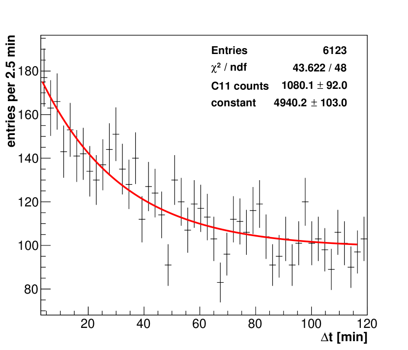
Figure 5: Example of a $\Delta t$ profile of ¹¹C-candidates following muons. The distribution contains an exponentially decaying component from correlated muon-¹¹C pairs as well as the flat component from accidental coincidences. In this special case, a lateral distance cut of $d_{\mu}=[1.0;1.2)\text{ m}$ is applied. The ratio of correlated to uncorrelated pairs is used to produce the probability profiles for the LH-TFC tagging shown in Fig. 6; in this case, the $6^{th}$ bin of histogram (b).

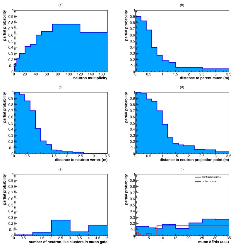
Figure 6: Overview of partial probability profiles of likelihood TFC discrimination parameters (description in the text).

We use a selection of seven discrimination parameters. The probability profiles obtained from the data for the first six are displayed in Figure 6:

• Neutron multiplicity, $p(n_{n})$: A higher number of neutrons, $n_{n}$, following a parent muon is a good indicator for hadronic shower formation. In some cases, a very luminous muon will flood the internal memories of the electronics, causing the NW to be entirely devoid of hits; based on a fit of the corresponding $\Delta t$-distribution (i.e. selecting only muons followed by no hits in the subsequent NW), we determine for this case a value of $p(n_{n})=0.885$, corresponding to a very high probability to find subsequent ¹¹C decays.

• Distance to the muon track, $p(d_{\mu})$: The probability to be ¹¹C is found to decline as function of $d_{\mu}$. In cases where muon track reconstruction fails, a probability $p(d_{\mu})$ of 0.182 is assigned (based on the corresponding subsample).

• Distance to the closest neutron vertex, $p(d_{n})$: Proximity to the neutron capture vertex was found to be a strong indicator for ¹¹C.

• Distance to the closest neutron projection point, $p(d_{np})$: Proximity to the projection of the vertex on the muon track was identified as a similarly efficient indicator.

• Neutrons in the MW, $p(n_{\mu n})$: While the entire MW in the wake of the initial muon signal is usually dominated by afterpulses, a special clustering algorithm has been devised to find superimposed peaks from cosmogenic isotopes and neutrons. While the vertex of these events cannot be reconstructed, the mere presence of these late clusters provides a (weak) indication of shower formation and hence ¹¹C production.

• $\mathbf{dE/dx}$ of the parent muon, $p(dE/dx)$: High energy deposition per unit muon path length is a good indicator for a muon-induced hadronic shower. Here, we consider the visible energy of the muon per total path length as an observational estimator for the physical quantity. Two different distributions are used, one describing muons that have crossed the scintillator volume (scintillator muons), the other for those passing it by (buffer muons).

• Time elapsed since muon, $p(\Delta t)$: The radioactive decay of ¹¹C means that a large time difference to the parent muon are less likely. The basic probability assigned is an exponential decay with the ¹¹C lifetime.

It is worthwhile to note that the partial profiles obtained do not constitute probability density functions in a mathematical sense. For instance, a good fraction of the accidental coincidences has been removed from the $\Delta t$ profiles by selecting only events inside the ¹¹C energy range and within a spherical volume of 3 m radius to remove both low-energy radioactive decays and external backgrounds. For some of the variables that only weakly select for ¹¹C (e.g. the muon dE/dx), it was necessary to apply additional cuts to a second discrimination parameter to further enhance the signal-to-background ratio. Finally, the integral of the distributions shown in Figure 6 are not normalized. However, this is of no practical consequence for the construction of the likelihood since the contribution of the $p_{i}$ are a posteriori tuned by weight factors $w_{i}$ (see below).

3.2.2 Construction of the likelihood

$j$	emphasis	$q_{j}$	$w(d_{\mu})$	$w(n_{n})$	$w(n_{\mu n})$	$w(d_{n})$	$w(d_{np})$	$w(\frac{dE}{dx})$	$w(\Delta t$)
1	closest $n$ vertex	0.025	1	1	0	2	0	0	1
2	closest $n$ proj.	0.436	1	1	0	0	1	0	1
3	neutrons in MW	0.740	1.5	0	1	0	0	1	1
4	high $n$-mult.	0.370	1.5	1	0	0	0	1	1

Table 1: The case-dependent likelihood implementations $(j=1..4)$ for TFC (see text): Probability offsets $q_{j}$ and weight factors $w_{ij}$ are listed.

The construction of a single likelihood ${\cal L}$ for a given ¹¹C candidate necessitates the expansion of the simple likelihood definition to the expression

$${\cal L}_{jk}=q_{j}\cdot\prod_{i}(p_{ik})^{w_{ij}},$$ (1)

where $\prod_{i}p_{ik}$ is the product of the probability values derived from the profiles shown in Fig. 6, with the index ($k$) denoting a specific parent muon. The meaning of the individual parameters $q_{j}$, $w_{ij}$ is explained below.

There are two considerations that drive us to building the likelihood in this way. First, each candidate can be associated to a large number of preceding muons, i.e. for each muon-candidate pair, an individual likelihood value ${\cal L}_{k}$ has to be computed. Second, the discrimination parameters feature different levels of indicative force for tagging ¹¹C. Moreover, some are statistically interdependent, some on the other hand contradictory: for instance, while the distances to the neutron vertex and projection, $p(d_{n})$ and $p(d_{np})$, are good ¹¹C indicators on their own, their product is likely to be large only for candidates at similar distance from both and thus highly misleading for the purpose of ¹¹C tagging.

To address these issues, the partial probabilities $p_{i}$ are weighted by exponents $w_{i}$ that re-scale their relative contribution to the calculation of $\cal L$. Note that the introduction of the weights $w_{i}$ does preserve the shapes of the individual probability profiles ($p_{i}$) shown in Fig. 6. In addition, we consider different implementations $(j)$ of the final likelihood, each one putting emphasis on a particular ¹¹C tagging strategy by re-weighing/excluding different sets of discrimination parameters ($i$):

• Proximity to a neutron vertex is given a special emphasis while the distance to the next projection point is not included.

• Proximity to a neutron projection point puts the tagging priority opposite of (1).

• Presence of neutrons in the MW bears the complication that no vertex reconstruction is available for neutrons in the MW. Thus, only the presence of neutrons and muon-related information is regarded.

• Muons featuring high neutron-multiplicities are usually very luminous, again impacting spatial reconstruction for the subsequent neutron vertices. Therefore, vertex information is not regarded for $n_{n}>20$, given instead larger emphasis to muon-related parameters.

The corresponding weights $w_{ij}$ are listed in Table 1 and are set to 0 if a specific $p_{i}$ is not to contribute to the likelihood.

Subsequently, the different implementations $(j)$ are evaluated and the variant providing the highest likelihood value ${\cal L}_{jk}$ is selected. To permit the direct comparison of the ${\cal L}_{jk}$, we have defined for each variant $(j)$ an optimum working point for what regards ¹¹C tagging efficiency and ¹¹C-depleted exposure. These figures of merit are introduced in Section 3.4. In order to compensate the differences in absolute scale, we apply a posteriori a scaling factor $q_{j}$ to each likelihood ${\cal L}_{jk}$, permitting a direct comparison between the four implementations $(j)$.

This procedure provides a single likelihood value ${\cal L}_{k}$ for a specific $\mu$-candidate pair. Also the likelihoods obtained for all possible parent muons $(k)$ are compared and again the maximum value is chosen. Thus, the final likelihood ${\cal L}$ for a specific ¹¹C candidate is

$${\cal L}={\rm max}_{k}\left[{\rm max}_{j}{\cal L}_{jk}\right].$$ (2)

All numerical values of the parameters listed in Table 1 have been optimized using the 2012 data set regarding tagging efficiency and preserved exposure (see Section 3.4). Like the partial probabilities $p_{i}$, the resulting $\cal L$ thus cannot be considered a likelihood in a strict mathematical sense. However, a high value of $\cal L$ is indeed a reliable indicator for the cosmogenic origin of an event.

3.2.3 Application as ¹¹C event classifier

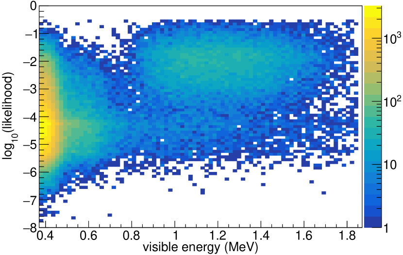
Figure 7: Distribution of TFC likelihood ${\cal L}$ as a function of visible energy. Two event populations can be identified. The upper band centered around ${\cal L}\sim 10^{-2}$ are ¹¹C decays concentrated in the ¹¹C energy range. Contrariwise, the lower band centered on ${\cal L}\sim 10^{-4}$ consists of neutrino events. It is worth to note that the large spectral excess of neutrino events at low energies only seems to suggest a vertical structure while it is in fact still centered around the same average value of ${\cal L}\sim 10^{-4}$. Based on the 2012 data set.

Differently from the HC-TFC, the LH-TFC provides the likelihood as a continuous variable for classification as a ¹¹C or neutrino event. The distribution of $\cal L$ as a function of the visible energy is shown in Figure 7. Indeed, two event categories are discernible: a neutrino band centered slightly below ${\cal L}\sim 10^{-4}$ and stretching over all visible energies; and a smaller cloud of events centered on ${\cal L}\sim 10^{-2}$ and concentrated in the energy range 0.75–1.87 MeV that can be associated with ¹¹C events. This is a demonstration that the likelihood ${\cal L}$ is indeed a potent classifier for ¹¹C events. Depending on the application, regions in this plot can be selected to either obtain a very pure ¹¹C or neutrino sample. The standard application for neutrino analyses is the introduction of an energy-independent cut at ${\cal L}_{0}=10^{-4}$ that removes the majority of the ¹¹C events, while keeping about 70% of the neutrino events. Analogously to the HC-TFC, this fraction is somewhat reduced when the Full Volume Vetoes discussed in the next section are applied in parallel.

3.3 Full Volume Regions

There are two situations in which the information on the parent muon and neutron events may be lost: during run breaks and during saturating muon events. These lead both algorithms to apply Full Volume Vetoes (FVV) to effectively reject potential ¹¹C events. We briefly describe them here.

Run Breaks.

The Borexino data taking is organized in runs with a programmed duration of 6 h although they can be shorter if automatically or manually restarted upon problems. The gap between runs can vary from a few seconds (ordinary restart) to one hour (weekly calibration) or exceptionally to a few days in case of major problems (blackouts, hardware failures). The gap between runs is a time where unrecorded muons could potentially generate ¹¹C in the scintillator which later decays after the run is restarted. TFC algorithms apply a FVV called After-Run-Break (ARB) veto: all events at the beginning of each run are tagged as potential ¹¹C without looking for the parenthood of muon-neutron pairs. The duration of the ARB veto is generally taken to be $\Delta t_{\textup{ARB}}=10+60\cdot(1-e^{-3\Delta t_{\textup{gap}}})$ min, where $\Delta t_{\textup{gap}}$ is the duration of the gap to the end of the previous run in minutes.

Showering muons.

Muons crossing several meters of scintillator and/or inducing hadronic showers are potentially generating multiple ¹¹C along the track. At the same time the high amount of light can provoke the saturation effects described in Section 2. This affects the position reconstruction of subsequent neutrons and can reduce the neutron detection efficiency in very extreme cases. Therefore, both algorithms apply a FVV after events with number of empty boards $N_{\rm EB}>N^{\rm thr}_{\rm EB}$ and $n_{n}>0$ for 4–5 $\tau_{{}^{11}\rm C}$. We observe that the average value of $N_{\rm EB}$ for non saturating events is slowly changing through the data set, mostly increasing due to the diminishing number of live channels. In addition a few rearrangement of the electronics and cabling also impacted on this parameter. In order to take this into account we adjust $N^{\rm thr}_{\rm EB}$ to a value above the bulk of the distribution in each subset of data defined by the same electronics configuration and let the outliers trigger the FVV.

It should be noted that the data within FVV are considered when TFC algorithms search for muon-neutron pairs.

FVV are very important to keep the tag efficiency high but have a high price in terms of exposure. This consideration led to the development of the alternative BI algorithm described in Section 4.

3.4 TFC Comparison

We present the performance of the two TFC algorithms described in terms of two desiderata. The TFC technqiue aims to maximize the ¹¹C tagging efficiency in the ¹¹C-enriched data set, while retaining the maximum exposure fraction in the ¹¹C-depleted set. The trade-off between those two competing requirements is ultimately decided by several parameters for the HC-TFC and by a single threshold ${\cal L}_{0}$ in case of the LH-TFC. While the working point we present here is the result of a careful optimization, the best parameter combinations for each neutrino analysis can be determined independently and may be to some extent different than what is presented here.

Exposure fraction.

The first figure of merit is the fraction of the exposure $\varepsilon_{\text{depleted}}$ that remains in the ¹¹C-depleted data set after TFC application. As laid out in Section 3, $\varepsilon_{\text{depleted}}$ is determined statistically by inserting random vertices (both position and time) into the experimental data stream and counting the fraction that is selected by the TFC criteria, i.e. would be included in the ¹¹C-depleted data set.

Tagging efficiency.

The second figure of merit is the tagging efficiency $e_{\text{tagged}}$. Its value is estimated based on a relatively narrow energy range from 1.2 to 1.4 MeV that is selected to minimize the presence of all spectral components but ¹¹C. In order to correct for the loss of live exposure in the depleted data set, $e_{\text{tagged}}$ is defined as:

$$e_{\text{tagged}}=1-\cfrac{\text{${}^{11}$C}_{\text{untagged}}}{\text{${}^{11}$C}_{\text{total}}}\,\cdot\cfrac{1}{\varepsilon_{\text{depleted}}}$$ (3)

where $\text{${}^{11}$C}_{\text{total}}$ and $\text{${}^{11}$C}_{\text{untagged}}$ are the total number of events and that of untagged events, respectively. It is worth noting that $e_{\text{tagged}}$ is actually a lower limit, as spectral analysis suggest a presence of $\sim$5% of non-¹¹C events in the evaluated energy range.

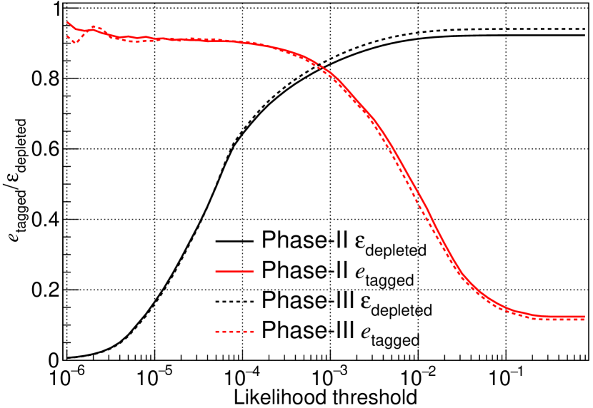
Figure 8: Performance of the LH-TFC as a function of its threshold value ${\cal L}_{0}$. ¹¹C tagging efficiency ($e_{\text{tagged}}$) and the exposure of the ¹¹C-depleted data set ($\varepsilon_{\text{depleted}}$) can be adjusted to the need of a particular analysis. For solar analysis, the default choice is ${\cal L}_{0}=10^{-4}$.

TFC tuning.

For both TFC algorithms a large flexibility of performance can be obtained tuning the selection parameters. In the case of the LH-TFC this is particularly easy as tagging efficiency and exposure can be varied as a function of the likelihood threshold ${\cal L}_{0}$ as shown in Figure 8. While a value of ${\cal L}_{0}=10^{-4}$ provides high tagging power for a moderate exposure loss that is ideal for solar neutrino analyses, a choice of ${\cal L}_{0}=10^{-2}$ would mean that a much larger fraction of the exposure would be preserved while only half of the ¹¹C candidates are tagged. In this case, the corresponding ¹¹C-enriched sample would almost exclusively consist of real ¹¹C decay events.

TFC performance.

The performance results are presented in Table 2 and are based on the data of Borexino Phase-II and Phase-III introduced in Section 2. Although the performance is essentially independent from the choice of the fiducial volume, for consistency we use the same fiducial volume of the $pep$ and CNO neutrino analyses (Section 2).

		Phase-II	Phase-III
Hard Cut	Tagging efficiency $(e_{\text{tagged}})$	90.2%	90.7%
	Exposure fraction $(\varepsilon_{\text{depleted}})$	63.3%	63.6%
Likelihood	Tagging efficiency $(e_{\text{tagged}})$	89.8%	90.1%
	Exposure fraction $(\varepsilon_{\text{depleted}})$	64.7%	65.6%

Table 2: Tagging efficiency (calculated with Equation 3) and exposure fraction for the two TFC approaches. For the LH-TFC, ${\cal L}_{0}$ is set at $10^{-4}$. The statistical uncertainty on all values of $e_{\text{tagged}}$ is 0.5%, while it is negligible on $\varepsilon_{\text{depleted}}$ values.

Both algorithms return a tagging efficiency of about 90% while providing a ¹¹C-depleted exposure fraction of $\sim$64%. While HC-TFC provides slightly better tagging, LH-TFC saves somewhat more exposure. In recent solar neutrino analysesbx_nusol , both algorithms have been applied separately to investigate potential differences in the corresponding spectral fit results and to assess systematic uncertainties.

Time stability.

We also investigated the stability of the TFC performance on a yearly bases throughout Borexino phase-II and III and extending till the end of 2020. In Figures 10 and 10 the ¹¹C tagging efficiency and the exposure fraction are shown for both TFC implementations. We attribute the slightly better performance of both TFC methods during Phase-III to a more continuous data taking which implies a lower impact of ARB cuts. Moreover, we observe a drift in LH-TFC performance during Phase-III, trading slightly lower tagging efficiencies for higher exposure fractions compared to HC-TFC. In principle, this trend could be compensated by a year-by-year adjustment of the likelihood threshold ${\cal L}_{0}$.

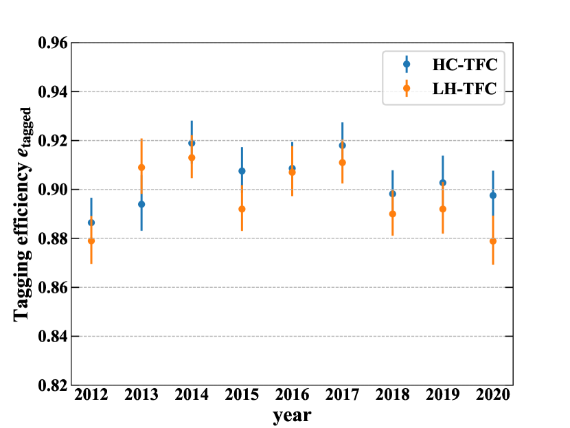
Figure 9: Tagging efficiency for HC-TFC (blue dots) and LH-TFC (orange dots) year by year.

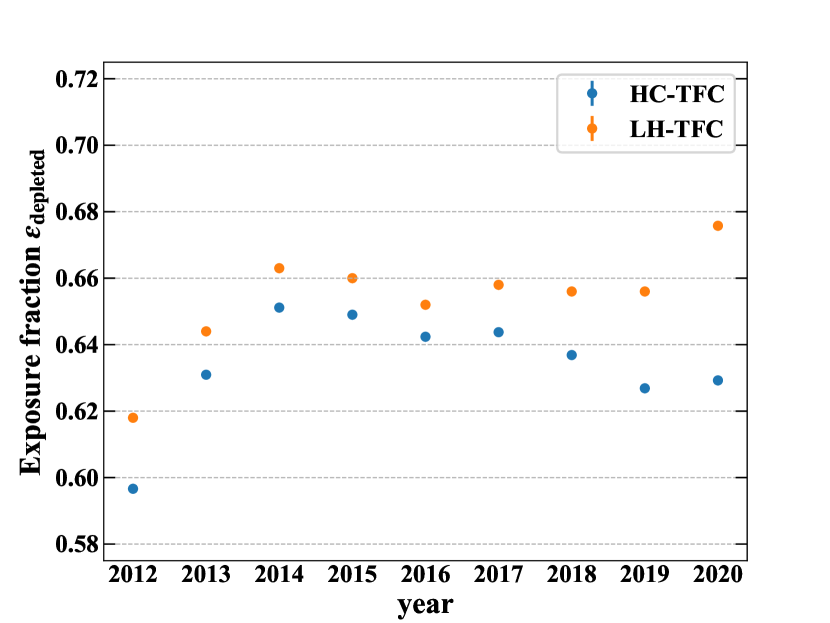
Figure 10: Exposure fraction of the depleted sample for HC-TFC (blue dots) and LH-TFC (orange dots) year by year.

4 ¹¹C burst Identification

The implementations of the TFC discussed so far have been extensively tested and validated and were part of several of the Borexino solar-$\nu$ analyses.

Here, we describe a novel method that further improves the identification of ¹¹C background events in Borexino and is potentially applicable as well to other large volume liquid scintillator detectors.

Most of ¹¹C is produced not by primary muon spallation but by secondary processes like $(p,n)$ reactions occurring in muon-induced hadronic showers. As a consequence, multiple ¹¹C nuclei are produced simultaneously in the detector and subsequently decay over a couple of hours. Consequently, identification of a burst of possible ¹¹C candidates correlated in space (i.e. along a hypothetical muon track) and time (several ¹¹C lifetimes) can provide a tag independent of any information on parent muon and neutron events. This is of particular interest since this Burst Identification (BI) tag will be available even if the initiating muon and/or subsequent neutron captures have been missed or misidentified by the data acquisition. Therefore, when applied in combination with either of the two TFC algorithms, the BI tag offers a more convenient alternative to the Full Volume Veto (FVV) introduced in Section 3.3.

The BI algorithm presented here proceeds first to identify groups of ¹¹C candidates, i.e. events in the correct energy window, with sufficient space and time correlation with each other. Once a burst has been identified, it is used to tag all events that show a correlation with the events that defined it.

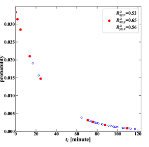
(a) Probability distribution from ¹¹C decay time in a $4\tau$ time window.

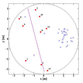
(b) Spatial distribution in the $xy$-plane.

Figure 11: Sample group of events considered for building a burst. Red full dots highlight the events that are finally selected as spatially correlated, with the multi-correlation factors $R^{2}$ reported in the legend in figure (a). The numbers in figure (b) reflect the time ordering (for clarity only some are shown). The dashed circle shows the radius of 3.5 m used to pre-select burst candidates. The dashed magenta line is the projection of the regression line. Open blue dots represent events not correlated with the first burst. Note that both panels show a late and spatially dense population belonging most likely to a second coinciding ¹¹C burst that is distinguished as separate by the algorithm.

4.1 Step 1: finding the burst

Time correlation.

The algorithm starts considering successively all ¹¹C candidates searching for time correlations. Candidate events are defined by a visible energy within 0.75–1.87 MeV corresponding to the ¹¹C spectrum. At this stage a very loose fiducial volume cut is applied: all events within a 3.5 m radius are considered. This has been optimized for excluding most of the external background events, without loosing many ¹¹C events that could be helpful in finding a burst. For each candidate, a subsequent time window corresponding to $4\tau_{{}^{11}\rm C}$ ($\sim$ 2 hours) is opened. In order to form a potential burst, at least four ¹¹C candidates have to be present inside the window (including the initial one). Figure 11 (a) shows a sample of events considered in the definition of a burst to whom we have associated a probability based on the exponential decay time of ¹¹C. We build a cumulative probability summing these values for all candidates, $\sum_{i}1/\tau_{{}^{11}\rm C}\cdot\exp(-(t_{i}-t_{0})/\tau_{{}^{11}\rm C})$, that is required to exceed a given threshold $p_{\text{th}}$. In the case of a run interruption within the observation window, this threshold is adjusted to take into account the dead time.

In some rare cases, it may happen that a burst falls within the selection window of a preceding unrelated ¹¹C candidate. The latter can then be mistaken as the first event and seriously distort the construction of the burst. In order to prevent this, we check whether the time distribution of events inside the selection window follows an exponential decay law. Specifically, if the time gap between first and second candidate is disproportionately large, the first event is considered unrelated to the burst and discarded.

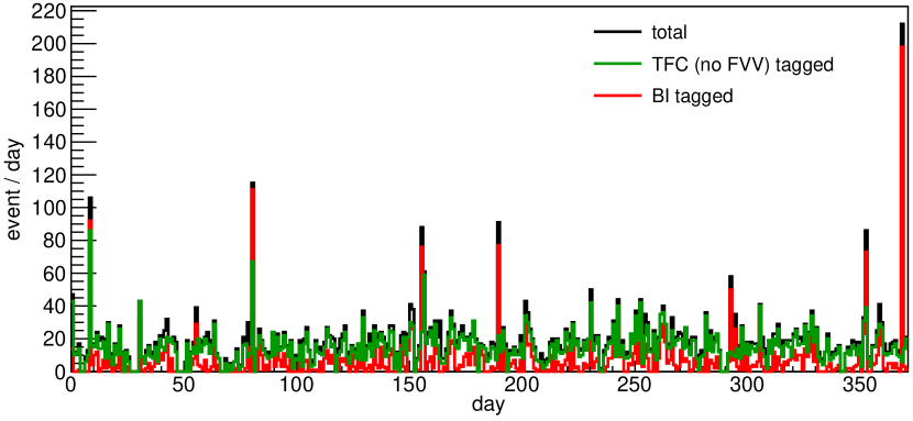
Figure 12: Events per day in the ¹¹C region inside the fiducial volume, in a year-long window of Phase-III. Black: total daily rate. Green: rate of events tagged by the TFC with the Full Volume Veto (FVV) switched off (see text for details). Red: rate of events tagged by the Burst Identification (BI) algorithm. Spikes in the rate correspond to bursts of ¹¹C.

Spatial correlation.

After a time correlation is established, the algorithm proceeds to check if any spatial correlation exists among the time-selected ¹¹C candidates. The basic assumption is that ¹¹C is produced and decays along a straight line (i.e. a muon track). Events that are far from this line are likely to be accidental time coincidences and must not be included in the burst. The hypothesis is tested via the correlation coefficients of the events coordinates upon projecting on the coordinate planes.

Figure 11 (b) shows the projection on the $(xy)$-plane of the sample events. Since the line is a freely oriented three-dimensional object, the use of classic Pearson correlation coefficients $\rho_{ij}=\text{cov}(i,j)/\sigma_{i}\sigma_{j}$ is not sufficient. Instead, the correlation is checked based on the three multi-correlation factors

$$R^{2}_{ij;k}=(\rho_{ik}^{2}+\rho_{jk}^{2}-2\rho_{ij}\rho_{ik}\rho_{jk})/(1-\rho_{ij}^{2})\text{,}$$ (4)

with $(i,j,k)$ denoting the different combinations of spatial coordinates $(x,y,z)$ that correspond to the coordinate planes.

Starting values for the $R^{2}_{ij;k}$ are computed based on the first four time-selected events (denoted as 0 to 3 in Figure 11). For each following event, the $R^{2}_{ij;k}$ values are re-computed after adding the event to the burst. The event is considered aligned with the track if: (1) all new $R^{2}_{ij;k}$ values remain larger than a given lower limit $R^{2}_{\text{lim}}$; (2) the two largest new $R^{2}_{ij;k}$ values do not differ from the previous values by more than a tolerance margin $R^{2}_{\text{tol}}$. Upon meeting both conditions the event is accepted to belong to the burst and the new $R^{2}_{ij;k}$ values become the new reference. In Figure 11 the events finally included in the burst after spatial selection are indicated by red filled circles. The final correlation factors $R^{2}_{{\rm burst};k}$ provide the thresholds for the application of the tagging (Section 4.2). The procedure is repeated upon sorting the events after their distance to the initial candidate and the case showing a stronger correlation is preferred.

For the performance evaluation presented in Section 4.3, the values of the parameters discussed above were chosen to be $p_{\text{th}}=0.12$, $R^{2}_{\text{lim}}=0.1$, and $R^{2}_{\text{tol}}=40\%$ (20%) for Phase-II (Phase-III). Although these parameter values are the result of a careful calibration of the algorithm, a different choice could be made in the context of a specific neutrino analysis in order to achieve a different trade-off between tagging efficiency and exposure fraction.

HC-TFC		Phase-II	Phase-III
no FVV	Tagging efficiency $(e_{\text{tagged}})$	79.5%	77.6%
	Exposure fraction $(\varepsilon_{\text{depleted}})$	70.8%	69.7%
no FVV + BI	Tagging efficiency $(e_{\text{tagged}})$	89.3%	90.4%
	Exposure fraction $(\varepsilon_{\text{depleted}})$	68.3%	66.7%
with FVV (standard)	Tagging efficiency $(e_{\text{tagged}})$	90.2%	90.7%
	Exposure fraction $(\varepsilon_{\text{depleted}})$	63.3%	63.6%

Table 3: Performance of the HC-TFC without Full Volume Veto (FVV) before and after the combination with the Burst Identification (BI) tag, compared with the standard HC-TFC already shown in Table 2. The statistical uncertainty on all values of $e_{\text{tagged}}$ is 0.5%, while it is negligible on $\varepsilon_{\text{depleted}}$ values.

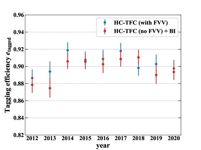
Figure 13: Tag efficiency year by year for TFC (with Full Volume Veto, FVV) and TFC (no FVV) + Burst Identification (BI), respectively in blue and red.

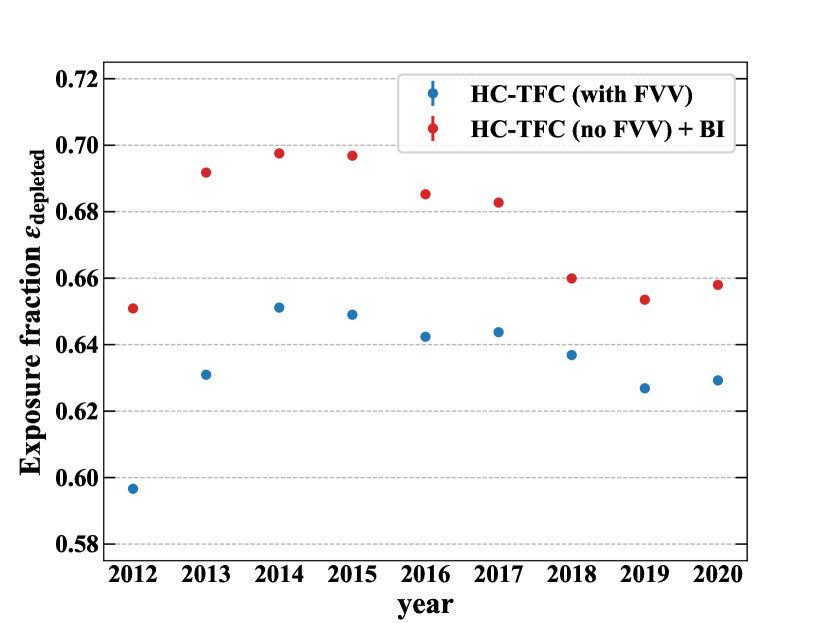
Figure 14: Exposure fraction of the depleted sample year by year for TFC (with FVV) and TFC (no FVV) + BI, respectively in blue and red.

4.2 Step 2: tagging the ¹¹C

Once a burst is identified by the events selected as in Section 4.1, all events within the burst time window, regardless of their energy, are checked for their affiliation with the burst and tagged as ¹¹C.

The track underlying the burst is found by a Theil-Sen regressiontheil ; sen returning the direction and the impact parameter based on the median of the tracks passing through all possible pairs of events of the burst (this method is less influenced by outliers compared to those based on the mean). In Figure 11 (b), the projection of the track on the $(xy)$-plane is shown as a magenta dashed line.

Thereafter, events within the burst time window are ordered by their distance to the track. Starting with the four closest events and then subsequently adding further events one by one, the algorithm proceeds to calculate the multi-correlation factors as in Equation 4. Newly added events are considered correlated with the track as long as all three $R^{2}_{ij;k}$ remain above the corresponding $R^{2}_{{\rm burst};k}$. Events may be tested for correlation multiple times if they fall within the time window of more than one track. An event is tagged as ¹¹C by the BI algorithm if it is correlated within at least one track.

Similarly to the TFC, the BI algorithm calculates the exposure fractions via toy Monte Carlo. Simulated events are uniformly distributed inside the fiducial volume and their correlation with all burst tracks is computed. The fraction of events for which $R^{2}_{ij;k}<R^{2}_{{\rm burst};k}$ for all tracks corresponds to the live exposure fraction.

4.3 BI Performance

As discussed in Section 3.3, the TFC algorithms can only identify ¹¹C decays for which the parent muon and subsequent neutrons have been detected. There are situations following breaks in data acquisition and especially very bright muon events saturating the electronics where this requirement is not satisfied. The Full Volume Vetoes (FVV) that have to be introduced to compensate for this deficiency are very costly in exposure for the ¹¹C-depleted sample. Here we demonstrate that the same task is more efficiently fulfilled by the BI algorithm.

Figure 12 shows the daily rate of events in the ¹¹C energy range and inside the fiducial volume (Section 2) over the course of a sample period of one year. It also shows the rates of those events identified as ¹¹C by the HC-TFC without FVV and of those identified by the BI algorithm. While this basic TFC identifies most of the ¹¹C events during regular data taking, it misses a larger fraction of events during the bursts due to exceptional high-multiplicity ¹¹C production. This behaviour is expected since ¹¹C-bursts are accompanied by severe saturation of the electronics. On the other hand, the BI algorithm shows heightened efficiency for these peak regions.

Hence, an event is assorted to the ¹¹C-enriched sample in case it is tagged either by the TFC (without FVV) or by the BI algorithm. Similarly, we evaluate the exposure based on a shared toy Monte Carlo generation. Results for the combined tagging efficiency and the ¹¹C-depleted exposure fraction are shown in Table 3. The combination shows a tagging efficiency similar to the full TFC (i.e. including FVV), but as expected it preserves a $\sim$3-5% larger exposure for the ¹¹C-depleted data set.

Similarly to Section 3.4, we have studied the time stability of the combined tags. The results are shown in Figures 14 and 14 for Phase-II, Phase-III, and extending until the end of 2020.

5 Conclusions

Low-energy neutrino detection in organic liquid scintillators suffers from spallation of carbon nuclei by cosmic muons. We have presented the state-of-the-art tagging and veto techniques for the most frequent spallation product ¹¹C that have been developed in Borexino in the context of solar $pep$ and CNO neutrino analyses.

We have described the Three-Fold Coincidence (TFC) technique that makes use of time and spatial correlation among parent muons, neutrons, and ¹¹C decay events. We have given details of its two current implementations, a Hard-Cut and a Likelihood-based approach. Scanning the data of Borexino Phases II (2012-2016) and III (2016-2020), we showed that both methods return stable results over a long time period. Typical tagging efficiencies exceed 90%, while the ¹¹C-depleted data set retains about 65% of the exposure.

Finally, we discussed the ¹¹C-burst tagging technique that exploits the fact that ¹¹C is often created in bursts by major spallation events. This novel approach searches for clusters of ¹¹C candidates that feature an exponentially decaying time behavior and are closely aligned along a track. We showed how this technique can be combined with the TFC and determined the corresponding improvement in surviving exposure fraction (66.7 % vs. 63.6%) for essentially the same tagging power on Phase-III data. Given the net benefit, the method is intended for use in future solar neutrino analyses of Borexino.

While native to Borexino, these methods can be easily adjusted to the identification and veto of other isotopes or to alternative experimental setups, and thus may be of benefit for a wide range of present and future low-energy neutrino and other low-background experiments.

- (1) G. Bellini, et al., Phys. Rev. Lett. 107, 141302 (2011). DOI 10.1103/PhysRevLett.107.141302
- (2) G. Bellini, et al., Phys. Rev. D 82, 033006 (2010). DOI 10.1103/PhysRevD.82.033006
- (3) G. Bellini, et al., Phys. Rev. Lett. 108, 051302 (2012). DOI 10.1103/PhysRevLett.108.051302
- (4) G. Bellini, et al., Nature 512(7515), 383 (2014). DOI 10.1038/nature13702
- (5) M. Agostini, et al., Nature 562(7728), 505 (2018). DOI 10.1038/s41586-018-0624-y
- (6) M. Agostini, et al., Phys. Rev. D 100(8), 082004 (2019). DOI 10.1103/PhysRevD.100.082004
- (7) M. Agostini, et al., Phys. Rev. D 101(6), 062001 (2020). DOI 10.1103/PhysRevD.101.062001
- (8) M. Agostini, et al., Nature 587, 577 (2020). DOI 10.1038/s41586-020-2934-0
- (9) M. Agostini, et al., Eur. Phys. J. C 80(11), 1091 (2020). DOI 10.1140/epjc/s10052-020-08534-2
- (10) M. Deutsch. Proposal to NSF for a Borexino Muon Veto. Massachusetts Institute of Technology (1996)
- (11) C. Galbiati, et al., Phys. Rev. C 71, 055805 (2005). DOI 10.1103/PhysRevC.71.055805
- (12) G. Bellini, et al., Phys. Rev. D 89(11), 112007 (2014). DOI 10.1103/PhysRevD.89.112007
- (13) S. Abe, et al., Phys. Rev. C 81, 025807 (2010). DOI 10.1103/PhysRevC.81.025807
- (14) V. Lozza, The SNO+ Experiment (2019), pp. 313–328. DOI 10.1142/9789811204296_0019
- (15) F. An, et al., J. Phys. G 43(3), 030401 (2016). DOI 10.1088/0954-3899/43/3/030401
- (16) J.F. Beacom, M.R. Vagins, Phys. Rev. Lett. 93, 171101 (2004). DOI 10.1103/PhysRevLett.93.171101
- (17) K. Abe, et al., (2011)
- (18) S.W. Li, J.F. Beacom, Phys. Rev. D 92(10), 105033 (2015). DOI 10.1103/PhysRevD.92.105033
- (19) M. Askins, et al., Eur. Phys. J. C 80(5), 416 (2020). DOI 10.1140/epjc/s10052-020-7977-8
- (20) G. Alimonti, et al., Nucl. Instrum. Meth. A 600, 568 (2009). DOI 10.1016/j.nima.2008.11.076
- (21) G. Bellini, et al., JCAP 08, 049 (2013). DOI 10.1088/1475-7516/2013/08/049
- (22) G. Bellini, et al., JINST 6, P05005 (2011). DOI 10.1088/1748-0221/6/05/P05005
- (23) M. Agostini, et al., JCAP 02, 046 (2019). DOI 10.1088/1475-7516/2019/02/046
- (24) P. Alvarez Sanchez, et al., Phys. Lett. B 716, 401 (2012). DOI 10.1016/j.physletb.2012.08.052
- (25) Y. Abe, et al., JHEP 10, 086 (2014). DOI 10.1007/JHEP02(2015)074. [Erratum: JHEP 02, 074 (2015)]
- (26) H. de Kerret, et al., JHEP 11, 053 (2018). DOI 10.1007/JHEP11(2018)053
- (27) H. Theil, Nederl. Akad. Wetensch. 53, 386 (1950)
- (28) P.K. Sen, Journal of the American Statistical Association 63(324), 1379 (1968). DOI 10.2307/2285891