Realization of multi-input/multi-output switched linear systems from Markov parameters

Abstract

This paper presents a four-stage algorithm for the realization of multi-input/multi-output (MIMO) switched linear systems (SLSs) from Markov parameters. In the first stage, a linear time-varying (LTV) realization that is topologically equivalent to the true SLS on intervals of interest is derived from the Markov parameters assuming that the discrete states have a common MacMillan degree and a mild condition on their dwell times holds. In the second stage, stationary point set of a Hankel matrix with fixed block column and row dimensions and built from the Markov parameters is examined. Splitting of this set into a union of disjoint intervals and intersection of their complements reveals linear time-invariant dynamics prevailing on these intervals. Absolute sum of modal eigenvalues is used as a feature for clustering to extract the discrete states, up to arbitrary similarity transformations. Recovery of the discrete states is complete if a mild unimodality assumption holds and each discrete state visits at least one segment and stays there long enough. In the third stage, the switching sequence is estimated by three schemes. The first scheme is based on correcting the state-space matrices estimated by the LTV realization algorithm from the Markov parameters. It starts from a discrete state estimate, proceeds along the positive and/or the negative real axes, and continues until a switch or a switch pair is detected. This process is repeated until all switches compatible with the dwell time requirements are detected. The second scheme is based on matching the estimated and the true Markov parameters of the SLS system over segments of the switching sequence. The third scheme is also based on matching the Markov parameters, but it is a discrete optimization/hypothesis testing algorithm. The three schemes operate on different dwell time and model structure requirements, but their dwell time requirements are weaker than the one needed to recover the discrete states. In the fourth stage, the discrete states estimated in the second stage are brought to a common basis by applying a novel basis transformation method which is necessary before performing output predictions to prescribed inputs. Robustness of this algorithm to amplitude bounded noise is studied and it is shown that small perturbations may only produce small deviations in the estimates that vanish as noise amplitude diminishes. Time complexity of the four-stage algorithm is also studied. A numerical example illustrates the derived results. A key role in this algorithm is played by a time-dependent switching sequence that partitions the state-space according to time, unlike many other works in the literature in which partitioning is state and/or input dependent.

[inst1]organization=Department of Automatic Control, addressline=Lund University, Box 117, postcode=SE-221 00, country=Sweden

[inst2]organization=Department of Electrical and Electronics Engineering,addressline=Eskisehir Technical University, city=Eskisehir, postcode=26555, country=Turkey

1 Introduction

Hybrid systems have attracted a vast interest lately due to their universal modeling capabilities of nonlinear dynamical systems. Switching among a finite set of linear submodels facilitated the difficult nonlinear identification problem into an identification of several affine submodels [1, 2] and has found its place in many versatile applications in video and texture segmentation [3, 4, 5], air traffic systems [6], human control behavior [7], and evolution of HIV infection [8].

Most works in hybrid systems literature abide to input-output representations, namely, piecewise auto-regressive exogenous (PWARX) and switched auto-regressive exogenous (SARX) modeling techniques [9, 10, 11, 12, 13, 14, 15] while especially in MIMO systems, state-space models are most preferred [16, 17]. Controllability, observability, fault detection, and observer design concepts are also well understood for state-space models. Equivalence between input-output and state-space models in hybrid systems was introduced in [18] by assuming pathwise observability. An SLS is inspired by classical state-space representation based on linear time-invariant (LTI) models and is characterized by its hard switching points between its possible operating subdynamics, unlike a linear parameter-varying (LPV) system whose model parameters most often change smoothly over time [19]. Actually, an SLS is nothing but an LPV system with non-smooth and abrupt changes [20]. Equivalence between SLSs and the LPVs was formally addressed in [21, 22] and a power series based algorithm was proposed for the realization of the latter which is actually the Ho-Kalman algorithm [23] adapted to these particular model structures. Markov parameters are useful to estimate state-space matrices describing best the underlying system dynamics when the system’s pulse response is known [24].

State-space SLS models are an important subclass of hybrid systems and their estimation is known to be a difficult problem since neither the knowledge of the data partitioning nor the submodels (discrete states) are available a priori. The continuous state is also unknown, which further obstructs treating it as a regression problem. Additionally, estimated state-space submodels reside in a different state basis, which hinders their use for output prediction to prescribed input signals [25]. A state-space realization algorithm for LPV input-output models was presented in [26]. Relationships between state-space models and auto-regressive exgoneous (ARX) and auto-regressive moving-average exogenous (ARMAX) input-output models were explored in [27] by introducing observer Markov parameters initially in LTI setting and later in LTV setting [28]. Complexity of the SLS identification process requires a set of assumptions on dwell times of the discrete states [29], observability [30], or knowledge of the switching sequence [31] which can be vital for the success of a proposed algorithm.

1.1 Related work

Methods that utilize subspace techniques to detect switches, identify active submodels between switches, and merge similar submodels to estimate a switching sequence were reported in [32, 33]. In [34], input-to-state-to-output measurements were assumed to be available and discrete state parameters were estimated by a sparsity-inducing optimization approach. A novel approach in [35] transformed identification problem into an SARX estimation problem by modulated output injection with observer deadbeat gains and discrete state parameters were estimated by minimizing a sparsity-promoting norm. An online structured subspace identification method equipped with a switch detection strategy was reported in [36]. An approximate expectation-maximization method for learning maximum-likelihood parameters of a linear switching system was proposed in [37], which might get stuck to a local minimum. This method was improved in [38] by adjusting search direction. Online approach proposed in [39] alternates between Markov parameter estimation and system classification to obtain local models.

The eigensystem realization algorithm (ERA) proposed in [40] is a noisy version of the famous Ho-Kalman algorithm [41]. It uses numerically robust, but expensive singular value decomposition (SVD) and returns a minimal balanced realization of the LTI system. A modified so-called ERA/DC algorithm was presented in [42] where data correlations rather than actual response values were used. The methodology here serves to average-out the effect of noise on the estimated state-space realization under the observation that output covariance matrices are identical to Markov parameter covariance matrices when the system is excited with white noise inputs. Online version of the ERA was reported in [43]. Extented version of the ERA dealing with arbitrary-variations was presented in [44] as a time-varying ERA (LTV-ERA).

1.2 Motivation for the SLS realization

This paper is about the realization of SLSs described by a discrete convolution equation

$$y(k)=h(k,l)\ast u(l)+e(k)\qquad k=1,\cdots,N$$ (1)

where $u(l)$ is the input, $h(k,l)$, $-\infty\leq l\leq k$ are the doubly indexed Markov parameters, $y(k)$ and $e(k)$ are respectively the output and noise. The collection $h(k,l)$, $l\leq k\leq N$ grows as $N$ increases. The state-space description in Section 2 provides a compact representation of (1) where the state-space matrices are assumed to change at switches.

The goal of system identification is to learn a model for (1) from the input-output data and provide a convergence guarantee, which is often asymptotic in $N$. Finite sample complexity issues have mostly been ignored in system identification literature. There is a surge of interest from the machine learning community in data-driven control and non-asymptotic analysis. In [45], sample complexity results in learning the Markov parameters from single trajectories of LTI systems were derived. On the same theme, but with an emphasis on the realization issue, further results were obtained in [46]. In contrast to LTI systems, relatively few results are available for the identification and the realization of SLSs in the state-space framework. Sparse optimization approach applied to SLS parameter estimation in [34, 35] has been a promising alternative to least-squares methods.

Realization theory for LPV systems is not complete despite many advances [21, 47, 22, 48]. The realization problem studied in this paper is an extension of a result derived in [35] to MIMO setting and draws on the early LTV realization results [49]. A key role in the realization is played by a time-dependent switching sequence that partitions the state-space according to time, unlike many other works in the literature in which partitioning is state and/or input dependent. In jump Markov linear systems, for example, switching sequence evolves according to a finite state Markov chain [50]. In a recent study [51], time-varying parameters were modeled as an output vector of a finite-dimensional linear system driven by the input-output data (1).

1.3 Organization of the paper

In Section 2, we formulate the SLS realization problem from finite Markov parameter sequences. Section 3 builds on the realization problem for MIMO-LTV systems from input-output data studied in [49]. It is demonstrated that under mild assumptions on the dwell times of the discrete states one can extract an LTV realization that is topologically equivalent to the true SLS on every time interval of sufficient length.

Section 4 starts by examining stationary point set of a Hankel matrix with fixed block and column dimensions and generated by the Markov parameters of the SLS. This is a special case of the sum-of-norms regularization method applied to the segmentation problem in SARX models [52] in which a parameter vector replaces the Hankel matrix. The switches of the SARX model are estimated in [52] by minimizing a quadratic norm of mismatch error regularized by a sum of parameter changes. On interval subsets of a stationary point set, an SLS behaves like an LTI system. It is demonstrated that every sufficiently long segment of a switching sequence contains an interval from the stationary point set if the discrete states satisfy a unimodality condition. This result paves the road for the proposal of a discrete state estimation algorithm based on clustering. Features used for clustering and clustering algorithms are briefly discussed. A feature based on absolute sum of modal eigenvalues used for clustering extracts all discrete states up to arbitrary similarity transformations if each discrete state visits at least one segment and dwells long enough there.

Sections 5 and 6 are devoted to estimation of the switching sequence. We present three schemes. The first scheme is based on correcting the state-space matrices estimated by the LTV realization algorithm from the Markov parameters. It starts from a discrete state estimate and proceeds along the positive and/or the negative real axes and continues until a switch or a switch pair is detected. This process is repeated until all switches, compatible with the dwell time requirements, are detected. The second scheme is based on matching the estimated and the true Markov parameters of the SLS system over a segment. This scheme too similarly starts from a discrete state estimate and proceeds along the positive and/or negative real axes until a switch or a switch pair is detected. The third scheme is also based on matching the Markov parameters, but it is a discrete optimization/hypothesis testing algorithm. The three switch detection schemes operate on different dwell time and model structure requirements, but their dwell time requirements are weaker than that one needed to recover the discrete states.

The discrete state estimates in Section 4 are only similar to the true ones. If they will be used for predicting outputs to prescribed inputs, it is necessary to bring them into a common basis with only one similarity transformation chosen freely. By exploiting minimality of the discrete states and putting a mild restriction on the minimum dwell time, we present an elegant solution to this problem in Section 7. In Section 8, we put all derivations together to form a meta-algorithm. Sensitivity analysis of this meta-algorithm to amplitude bounded noise is performed, more specifically it is shown that small perturbations in the Markov parameters may only lead to small deviations in the estimates that vanish as noise amplitude diminishes. Time complexity of each stage in the meta-algorithm is studied in detail. A numerical example in Section 9 illustrates the derived results. Section 10 concludes the paper.

2 Problem formulation

In this paper, we consider a class of MIMO–LTV systems represented by the state-space equations

$$x(k+1) = A(k)x(k)+B(k)u(k),$$ (2)

$$y(k) = C(k)x(k)+D(k)u(k)$$ (3)

where $u(k)\in\mathbb{R}^{m}$, $y(k)\in\mathbb{R}^{p}$, and $x(k)\in\mathbb{R}^{n}$, $k=1,\cdots,N$ are respectively the input, the output, and the state sequences. The state dimension $n$ is constant and assumed to be known.

Let $\mathbb{N}$ denote the set of positive integers and $\varphi$ be a switching sequence, that is, a map from $\mathbb{N}$ onto a finite set $\mathbb{S}=\left\{1,\cdots,\sigma\right\}$ with a fixed and known $\sigma\in\mathbb{N}$. Let ${\mathcal{P}}(k)=(A(k),B(k),C(k),D(k))$ for $k=1,\cdots,N$. Since $\varphi(k)\in\mathbb{S}$ for all $k$, we define the collection of the discrete states by ${\mathcal{P}}=\left\{{\mathcal{P}}_{1},\cdots,{\mathcal{P}}_{\sigma}\right\}.$ The MIMO–LTV system (2)–(3) with the state-space matrices changed by $\varphi$ is an SLS. The switching sequence $\varphi(k)$ partitions $[1\;\;N]$ to a collection of disjoint intervals $[1\;\;k_{1})$, $[k_{i}\;\;k_{i+1}),\,\cdots,\,[k_{i^{*}}\;\;N]$ such that

$$\varphi(k)=\left\{\begin{array}[]{l}\varphi(1),\qquad 1\leq k<k_{1}\\ \varphi(k_{i}),\qquad k_{i}\leq k<k_{i+1}\\ \varphi(k_{i^{*}}),\qquad k_{i^{*}}\leq k<N.\end{array}\right.$$ (4)

Denoting this segmentation by $\chi$, we define the dwell times $\delta_{i}(\chi)$ and the minimum dwell time $\delta_{*}(\chi)$ by

$$\delta_{i}(\chi)=k_{i+1}-k_{i}\;\;\;\mbox{and}\;\;\;\delta_{*}(\chi)=\min_{1\leq i<i^{*}}\delta_{i}(\chi).$$ (5)

Thus, $\delta_{i}(\chi)$ is the waiting time of the discrete state active in the segment $[k_{i},k_{i+1})$ and $\delta_{*}(\chi)$ is the smallest waiting time of all discrete states in the interval $[1\;\;k_{i^{*}})$. Set $\delta_{0}(\chi)=k_{1}-1$ and $\delta_{i^{*}}(\chi)=N-k_{i^{*}}$.

By introducing the Markov parameters and the state transition matrix associated with the homogeneous part of (2) defined respectively by

$$h(k,\ell)=\left\{\begin{array}[]{ll}C(k)\Phi(k,\ell+1)B(\ell),&k>\ell\\ D(k),&k=\ell\\ 0,&k<\ell,\end{array}\right.$$ (6)

and

$$\Phi(k,\ell)=\left\{\begin{array}[]{ll}A(k-1)\,\cdots\,A(\ell),&k>\ell\\ I_{n},&k=\ell\end{array}\right.$$ (7)

where $I_{n}\in\mathbb{R}^{n\times n}$ is the identity matrix, from (2)–(3), we can calculate the response of the system to any initial state $x(\ell)$, $\ell\geq 1$ and a prescribed input sequence $u(k)$, $k\geq 1$ as follows

$$y(k)=C(k)\Phi(k,\ell)x(\ell)+\sum_{j=\ell}^{k}h(k,j)u(j),\;\;\;\ell\leq k\leq N.$$ (8)

Since the state-space matrices are changed by the switching sequence, the input-output trajectory of (2)–(3) strongly depends on $\varphi$. In most works on SLSs, $\varphi$ is a typically state or/and input dependent signal whereas in the current work it is an unknown signal. The realization problem we study in this paper is described as follows.

Problem 2.1.

Given a set of doubly indexed Markov parameters $h(k,\ell)$ of the MIMO–SLS model (2)–(4) for $1\leq k\leq N$ and $1\leq\ell\leq k$ , estimate each ${\mathcal{P}}_{j}\in{\mathcal{P}}$, $j=1,\cdots,\sigma$ up to a similarity transformation and $\varphi(k)$.

In the course of developing a realization algorithm that solves Problem 2.1, we will impose some conditions on the system structure and the switching sequence. We will also discuss the freedom in choosing similarity transformation.

3 LTV realization from Markov parameters

This section prepares the stage for a discrete-state estimation algorithm and three switch detection schemes presented in Sections 4, 5, 6, and 6.3. In this section, we will review the realization problem for MIMO-LTV systems from input-output data. Recall that the description of an LTV system in terms of state-space matrices is not unique: Two given realizations $(A,B,C,D)$ and $(\check{A},\check{B},\check{C},\check{D})$ have the same Markov parameters if they are topologically equivalent, i.e., there exists a bounded $T(k)\in\mathbb{R}^{n\times n}$ with bounded inverse such that for all $k\in\mathbb{N}$,

$$\check{A}(k)=T(k+1)A(k)T^{-1}(k),\qquad\check{B}(k) = T(k+1)B(k),$$

$$\check{C}(k)=C(k)T^{-1}(k),\qquad\check{D}(k) = D(k).$$

We call $T(k)$ a Lyapunov transformation. As far as input-output behavior is concerned, it suffices to estimate the Markov parameters from input-output data.

Let $q,r\in\mathbb{N}$ be two numbers to be fixed later. For all $k>r$, we define the Hankel matrices by

$${\mathcal{H}}_{q,r}(k)=\left[\begin{array}[]{ccc}h(k,k-1)&\cdots&h(k,k-r)\\ &\ddots&\vdots\\ &\cdots&h(k+q-1,k-r)\end{array}\right]$$ (9)

which can be factorized from [49] as follows

$${\mathcal{H}}_{q,r}(k)={\mathcal{O}}_{q}(k)\,{\mathcal{R}}_{r}(k-1)$$ (10)

with ${\mathcal{O}}_{q}(k)$ and ${\mathcal{R}}_{r}(k-1)$ denoting the extended observability and the controllability matrices defined by

$${\mathcal{O}}_{q}(k)=\left[\begin{array}[]{c}C(k)\\ C(k+1)\Phi(k+1,k)\\ \vdots\\ C(k+q-1)\Phi(k+q-1,k)\end{array}\right]\in\mathbb{R}^{qp\times n}$$ (11)

and

$${\mathcal{R}}_{r}(k-1)=\left[B(k-1)\;\;\cdots\;\;\Phi(k,k-r+1)B(k-r)\right].$$ (12)

The observability and the controllability Gramians for the LTV system (2)–(3) are defined by

$${\mathcal{G}}_{\rm o}(k;q) = {\mathcal{O}}_{q}(k)^{T}{\mathcal{O}}_{q}(k)$$ (13)

$${\mathcal{G}}_{\rm c}(k;r) = {\mathcal{R}}_{r}(k-1){\mathcal{R}}_{r}^{T}(k-1)$$ (14)

If $A(k),B(k),C(k)$ are bounded matrices for all $k$, $(A(k),B(k),C(k))$ is said a bounded realization. A bounded realization $(A(k),B(k),C(k))$ is uniformly observable iff $A(k)$ is nonsingular and $\exists\,q\in\mathbb{N}$ such that ${\mathcal{G}}_{\rm o}(k;q)\geq\alpha_{\rm o}I_{n}$ for some $\alpha_{\rm o}>0$ and $\forall k$. This fact is a restatement of Lemma 2 in [49] with changes in the notation. Similarly, a bounded realization $(A(k),B(k),C(k))$ is uniformly controllable iff $A(k)$ is nonsingular and $\exists\,r\in\mathbb{N}$ such that ${\mathcal{G}}_{\rm c}(k;r)\geq\alpha_{\rm c}I_{n}$ for some $\alpha_{\rm c}>0$ and $\forall k$. This fact restates Lemma 1 in [49] with appropriate changes in the notation. The following definition is adapted from [49].

Definition 3.1.

A bounded realization $(A(k),B(k),C(k))$ is uniform if it is uniformly observable and controllable.

For a bounded realization $(A(k),B(k),C(k))$, the definitions of uniformly observable, uniformly controllable, and uniform applies to all $k\in\mathbb{N}$. However, our observation interval is limited to $[1\;\;N]$. Moreover from (11) and (12), $k$ must satisfy the inequalities $k+q-1\leq N$ and $k-r\geq 1$. Hence, the above definitions can only be checked for all $k\in[r+1\;\;N-q+1]$. It is our best interest to pick $q$ and $r$ as small as possible while ${\mathcal{G}}_{\rm o}(k;q)$ and ${\mathcal{G}}_{\rm c}(k;r)$ are positive-definite. For fixed $k$, ${\mathcal{G}}_{\rm o}(k;q)$ and ${\mathcal{G}}_{\rm c}(k;r)$ are non-decreasing functions of $q$ and $r$, i.e., ${\mathcal{G}}_{\rm o}(k;q_{1})\geq{\mathcal{G}}_{\rm o}(k;q_{2})$ iff $q_{1}\geq q_{2}$ and ${\mathcal{G}}_{\rm c}(k;r_{1})\geq{\mathcal{G}}_{\rm c}(k;r_{2})$ iff $r_{1}\geq r_{2}$.

Observability is a critical aspect in observer design and identification algorithms for SLSs. Several observability definitions for SLSs (mode observability, strong mode observability, observability, strong observability etc.) have appeared in hybrid systems literature. Checking observability for SLSs is formidable. For example, checking the observability of (2)–(4) for all possible discrete state sequences of length $N$ can involve $O(\sigma^{N})$ rank tests. To deal with this exponential complexity, in [53] switching times were assumed to be separated by a minimum dwell time that depends on $n$. Under this assumption, computational complexity was shown to reduce from $O(\sigma^{N})$ to $O(\sigma^{2})$. The minimum dwell time is not very restrictive since rapidly changing modes may cause instability problems [25].

Bounded realization assumption follows from the following.

Assumption 3.1.

Every discrete state ${\mathcal{P}}_{j}\in{\mathcal{P}}$, $1\leq j\leq\sigma$ is bounded-input/bounded-output (BIBO) stable and has a Macmillan degree $n$. $\hfill\blacksquare$

We also impose a mild restriction on the minimum dwell time as follows.

Assumption 3.2.

The switching sequence $\varphi$ satisfies $\delta_{*}(\chi)\geq n$. $\hfill\blacksquare$

The following result was derived in [35].

Lemma 3.1.

Suppose Assumptions 3.1–3.2 hold and $q,r\geq 2n$. Then, the MIMO-SLS model (2)–(4) is uniform on $[2n+1\;\;N-2n+1]$. $\hfill\blacksquare$

This lemma enables one to extract an LTV realization which is topologically equivalent to (2)–(4) from the pairs $\{{\mathcal{H}}_{q,r}(k),{\mathcal{H}}_{q,r}(k+1)\}$, $k>r$. In fact, uniform realization property implies that ${\mathcal{O}}_{q}(k)$ and ${\mathcal{R}}_{r}(k-1)$ are full-rank matrices and the relationship ${\rm rank}({\mathcal{H}}_{q,r}(k))=n$ holds from an application of the Sylvester inequality [54] to the product in (10). The extended observability and controllability matrices are then determined up to similarity transformations from the SVDs of ${\mathcal{H}}_{q,r}(k)$ and ${\mathcal{H}}_{q,r}(k+1)$. In fact, let $J_{\uparrow}$ and $J_{\downarrow}$ denote the shift matrices of block-row up and down and $J_{\leftarrow}$ and $J_{\rightarrow}$ denote the block-column left and right shift matrices, respectively, defined by

$$J_{\uparrow}=\left[0_{(q-1)p\times p}\;\;I_{(q-1)p}\right],\;\;\;J_{\downarrow} = \left[I_{(q-1)p}\;\;0_{(q-1)p\times p}\right],$$ (15)

$$J_{\leftarrow}=\left[\begin{array}[]{l}0_{m\times(r-1)m}\\ I_{(r-1)m}\end{array}\right],\;\;\;J_{\rightarrow} = \left[\begin{array}[]{l}I_{(r-1)m}\\ 0_{m\times(r-1)m}\end{array}\right]$$ (20)

where $0_{m\times n}$ denotes the $m$ by $n$ matrix of zeros. Then, from the factorization formula (10) with $k$ and $k+1$ plugged in and (15)–(20) we derive the following relations

$$J_{\uparrow}{\mathcal{O}}_{q}(k) = \left(J_{\downarrow}{\mathcal{O}}_{q}(k+1)\right)A(k)={\mathcal{O}}_{q-1}(k+1)A(k)$$ (21)

$${\mathcal{R}}_{r}(k)J_{\leftarrow} = A(k)\left({\mathcal{R}}_{r}(k-1)J_{\rightarrow}\right)=A(k){\mathcal{R}}_{r-1}(k-1).$$ (22)

Hence, from (21) and/or (22) depending on if $q>2n$ and/or $r>2n$, we retrieve $A(k)$ from either/both of the formulas

$$A(k) = {\mathcal{O}}_{q-1}^{{\dagger}}(k+1)J_{\uparrow}{\mathcal{O}}_{q}(k)={\mathcal{R}}_{r}(k)J_{\leftarrow}{\mathcal{R}}_{r-1}^{{\dagger}}(k-1)$$ (23)

where $X^{\dagger}$ denotes the unique left or right-inverse of a given full-rank matrix $X$ defined as $(X^{T}X)^{-1}X^{T}$ or $X^{T}(XX^{T})^{-1}$ depending on the context. We fix $q$ and $r$ as $q=2n+1$ and $r=2n$. Then, $k>2n$. For an upper bound on $k$, the maximum block-row index of ${\mathcal{H}}_{qr}(k+1)$ must satisfy $k+q\leq N-2n+1$ or $k\leq N-4n$. Hence, $k^{\prime}\leq k\leq k^{\prime\prime}$ where $k^{\prime}=2n+1$ and $k^{\prime\prime}=N-4n$.

It remains to estimate ${\mathcal{O}}_{q}(k)$ and ${\mathcal{O}}_{q}(k+1)$. We apply SVD to ${\mathcal{H}}_{q,r}(k)$ and ${\mathcal{H}}_{q,r}(k+1)$

$${\mathcal{H}}_{q,r}(k) = U_{q}(k)\Sigma(k)V_{r}^{T}(k),$$

$${\mathcal{H}}_{q,r}(k+1) = U_{q}(k+1)\Sigma(k+1)V_{r}^{T}(k+1)$$

and let

$$\hat{\mathcal{O}}_{q}(k)=U_{q}(k)\Sigma^{1/2}(k),\;\;\;\hat{\mathcal{R}}_{r}(k-1) = \Sigma^{1/2}(k)V_{r}^{T}(k),$$ (25)

$$\hat{\mathcal{O}}_{q}(k+1)=U_{q}(k+1)\Sigma^{1/2}(k+1),\;\;\;\hat{\mathcal{R}}_{r}(k) = \Sigma^{1/2}(k+1)V_{r}^{T}(k+1).$$ (26)

Up to similarity transformations $T(k)$ and $T(k+1)$, $\hat{\mathcal{O}}_{q}(k)$ and $\hat{\mathcal{O}}_{q}(k+1)$ provide estimates of ${\mathcal{O}}_{q}(k)$ and ${\mathcal{O}}_{q}(k+1)$, i.e., ${\mathcal{O}}_{q}(k)=\hat{\mathcal{O}}_{q}(k)T(k)$ and ${\mathcal{O}}_{q}(k+1)=\hat{\mathcal{O}}_{q}(k+1)T(k+1)$. Let

$$\hat{A}(k)=\left(J_{\downarrow}\hat{\mathcal{O}}_{q}(k+1)\right)^{{\dagger}}J_{\uparrow}\hat{\mathcal{O}}_{q}(k)$$ (27)

so that

$$\hat{A}(k)=T(k+1)A(k)T^{-1}(k).$$ (28)

The estimation of $B(k)$ and $C(k)$ is in order. To this end, let

$$J_{\rm C}=\left[I_{p}\;\;O_{p\times(q-1)p}\right],\;\;\;J_{\rm B}=\left[\begin{array}[]{l}I_{m}\\ 0_{(r-1)m\times m}\end{array}\right].$$ (29)

Then, from (11) and (12)

$$C(k)=J_{\rm C}{\mathcal{O}}_{q}(k),\;\;\;B(k)={\mathcal{R}}_{r}(k)J_{\rm B}.$$ (30)

As the estimates of $C(k)$ and $B(k)$, we set

$$\hat{C}(k)=J_{\rm C}\hat{\mathcal{O}}_{q}(k),\;\;\;\hat{B}(k)=\hat{\mathcal{R}}_{r}(k)J_{\rm B}.$$ (31)

Then, from $\hat{\mathcal{R}}_{r}(k)=T(k+1){\mathcal{R}}_{r}(k)$,

$$\hat{C}(k)=C(k)T^{-1}(k),\;\;\;\hat{B}(k)=T(k+1)B(k).$$ (32)

Set $\hat{D}(k)=h(k,k)$. Then, from (28) and (32) it follows that $\hat{\mathcal{P}}(k)=(\hat{A}(k),\hat{B}(k),\hat{C}(k),\hat{D}(k))$ is topologically equivalent to ${\mathcal{P}}(k)$ on the interval $[k^{\prime}\;\;k^{\prime\prime}]$.

If $T(k)=T(k+1)$, $\hat{A}(k)$ is similar to $A(k)$ denoted by the notation $\hat{A}(k)\sim A(k)$. It is the case when $H_{q,r}(k)$ equals $H_{q,r}(k+1)$. For an LTI system, i.e., $\sigma=1$ in Assumption 3.1, $\hat{A}(k)\sim A(k)$. The derivations in this section are outlined in Appendix as a subspace-based realization algorithm. The realization returned by Algorithm 1 is topologically equivalent to (2)–(4). The quadruples returned are not similar to ${\mathcal{P}}(k)$, yet match the Markov parameters. Matching the discrete states will be achieved by modifying the state-space matrices as described in Section 5.

The LTV realization problem was studied in [28] from a rigid body dynamics perspective. The scheme presented above is based on single input-output data batches. If an ensemble of input-output data are available, state-space models can be identified without constraints on time-variations of the Markov parameters [55, 56]. The derivations above are summarized in the following result.

Theorem 3.1.

Consider Algorithm 1 with the noiseless Markov parameters of (2)–(4) satisfying Assumptions 3.1–3.2. Then, Algorithm 1 returns a realization topologically equivalent to (2)–(4) on $[k^{\prime}\;\;k^{\prime\prime}]$. $\hfill\blacksquare$

Notice that ${\mathcal{H}}_{q,r}(k+1)$ is formed from the $4n$ Markov parameters and a submatrix of ${\mathcal{H}}_{q,r}(k)$. In fact, partition $\mathcal{H}_{q,r}(k)$ as follows

$${{\cal H}_{q,r}}(k)=\left[{\begin{array}[]{*{20}{c}}{h(k,k-1)}&\cdots&{h(k,k-r)}\\ {{\cal H}_{q,r}^{\prime}(k)}&{}\hfil&\vdots\\ {}\hfil&{}\hfil&{h(k+q-1,k-r)}\end{array}}\right]$$ (33)

and observe that

$${\mathcal{H}}_{q,r}(k+1)=\left[\begin{array}[]{ccc}h(k+1,k)&&\\ \vdots&&{\mathcal{H}}_{qr}^{\prime}(k)\\ h(k+q,k)&\cdots&h(k+q,k-r+1)\end{array}\right].$$ (37)

Algorithm 1 uses $qr+(q+r-1)(k^{\prime\prime}-k^{\prime}+1)$ Markov parameters if it computes $\hat{\mathcal{P}}(k)$ for all $k\in[k^{\prime}\;\;k^{\prime\prime}]$ and if it computes for one $k$, $qr+q+r-1$ Markov parameters. Plug $q=2n+1$ and $r=2n$ in: $(4N-20n+2)n\approx 4Nn$ and $4n^{2}+6n\approx 4n^{2}$. If $\hat{\mathcal{P}}(k)$ is computed at every $2n+1$th sample, $(4n^{2}+6n)(k^{\prime\prime}-k^{\prime}+1)/(2n+1)\approx 2Nn$ Markov parameters roughly will be used since ${\cal H}_{2n+1,2n}(k)$ and ${\cal H}_{2n+1,2n}(k+2n)$ share no common entries. Hence, more than 50% of the Markov parameters need to be stored if calculations are done more frequently than $O(n)$. The algorithms developed in the sequel will need all Markov parameters to be stored. Time complexity of Algorithm 1, however, depends on the frequency of calculations as the following analysis demonstrates.

3.1 Time complexity of Algorithm 1

In Algorithm 1, calculation of the SVDs in (LABEL:svdHqr) is computationally the most expensive step without exploiting the block matrix structure and the nesting property in (33)–(37). According to [57], the best algorithms for SVD computation of an $M\times L$ matrix have time complexity $O(c_{1}M^{2}L+c_{2}L^{3})$ where $c_{1},c_{2}>0$ are absolute constants which are $4$ and $22$ for an algorithm called R-SVD. Recall that $q=2n+1$ and $r=2n$, from $M=qp$ and $L=rm$. Each SVD in (LABEL:svdHqr) has then a time complexity $O(poly(n))$ where $poly(n)$ is a third order polynomial in $n$. Pseudo-inverse of an $M\times L$ ($M>L$) matrix calculated by SVD has complexity $O(LM^{2})$. Hence, with $M=(q-1)p$ and $L=n$, $\left(J_{\downarrow}\hat{\mathcal{O}}_{q}(k+1)\right)^{{\dagger}}$ in (27) has complexity $O(n^{3})$. Multiplication of two matrices $X\in\mathbb{R}^{M\times K}$ and $Y\in\mathbb{R}^{K\times L}$ has complexity $O(MKL)$ when calculated directly. Hence, with $M=n$, $K=(q-1)p$, $L=n$ we get $O(poly(n))$ for the complexity of multiplication $\left(J_{\downarrow}\hat{\mathcal{O}}_{q}(k+1)\right)^{{\dagger}}$ times $J_{\uparrow}\hat{\mathcal{O}}_{q}(k)$. Adding up we get $O(poly(n))$ for the complexity of $\hat{A}(k)$. Since $J_{\rm B},\hat{\mathcal{R}}_{r}(k),J_{\rm C},\hat{\mathcal{O}}_{q}(k)$ are $n\times rm$, $rm\times m$, $p\times qp$, $qp\times n$ matrices respectively, applying the complexity result to the matrix multiplications in (31) we derive $O(poly(n))$ for the complexities of $\hat{B}$ and $\hat{C}$ where $poly(n)$ is a second order polynomial in $n$. It follows that $\hat{\mathcal{P}}(k)$ has complexity $O(poly(n))$ where $poly(n)$ is a third order polynomial. Denote the number of the elements in $\kappa$ by $|\kappa|$. Then, Algorithm 1 has time complexity $O(|\kappa|poly(n))$. Hence, Algorithm 1 subject to Assumption 3.2 has a worst-case time complexity $O(Npoly(n))$ where $poly(n)$ is a second order polynomial since $|{\mathcal{K}}|=O(Nn^{-1})$ for evenly distributed switches. If ${\mathcal{K}}$ is a singleton, then time complexity of Algorithm 1 will be $O(poly(n))$ with $poly(n)$ a third order polynomial in $n$. These calculations took into consideration only $n$ and $N$ since $p$ and $m$ are fixed small numbers. There is also a similar concept called space complexity which is usually weaker than time complexity. In the setting of this paper, for example, the SVD has space complexity $O(n^{2})$.

3.2 Robustness of Algorithm 1

Suppose that the Markov parameters in (6) are corrupted by ‘unknown-but-bounded’ type noise

$$\tilde{h}(k,\ell)=h(k,\ell)+e(k,\ell),\qquad\ell\leq k\;\;\;\mbox{and}\;\;\;k^{\prime}\leq k\leq k^{\prime\prime}$$ (38)

where $\|e(k,\ell)\|_{F}\leq\varepsilon$ with $\|\cdot\|_{F}$ denoting the Frobenius norm of a given matrix defined as the square root of the sum of its squared elements. Our goal is to study how this noise affects the estimates $\hat{\mathcal{P}}(k)$, $k\in[k^{\prime}\;\;k^{\prime\prime}]$ for small $\varepsilon>0$.

Let $\tilde{\mathcal{H}}_{2n+1,2n}(k)$ be the Hankel matrix obtained by populating ${\mathcal{H}}_{2n+1,2n}(k)$ in (9) with $\tilde{h}(k,\ell)$. Split $\tilde{\mathcal{H}}_{2n+1,2n}(k)$

$$\tilde{\mathcal{H}}_{2n+1,2n}(k)={\mathcal{H}}_{2n+1,2n}(k)+E(k).$$ (39)

Robustness of Algorithm 1 to unknown-but-bounded type noise follows from the following result.

Theorem 3.2.

Consider (2)–(4) with the noisy Markov parameters in (38). Suppose that Assumptions 3.1–3.2 hold. Let $\tilde{\mathcal{P}}(k)=(\tilde{A}(k),\tilde{B}(k),\tilde{C}(k),\tilde{D}(k))$ and $\hat{\mathcal{P}}(k)=(\hat{A}(k),\hat{B}(k),\hat{C}(k),\hat{D}(k))$ denote the models estimated by Algorithm 1 in the noisy and noiseless cases. Then, there exists a realization ${\mathcal{P}}^{\varepsilon}(k)=(A^{\varepsilon}(k),B^{\varepsilon}(k),C^{\varepsilon}(k),D^{\varepsilon}(k))$ that is topologically equivalent to $\tilde{\mathcal{P}}(k)$ satisfying $\|A^{\varepsilon}(k)-\hat{A}(k)\|_{F}\leq c\varepsilon$, $\|B^{\varepsilon}(k)-\hat{B}(k)\|_{F}\leq c\varepsilon$, $\|C^{\varepsilon}(k)-\hat{C}(k)\|_{F}\leq c\varepsilon$, $\|D^{\varepsilon}(k)-\hat{D}(k)\|_{F}\leq c\varepsilon$ for all $\varepsilon\leq\varepsilon_{*}$ and some $c,\varepsilon_{*}>0$. The Lyapunov transformation $S(k)$ mapping $\tilde{\mathcal{P}}(k)$ to ${\mathcal{P}}^{\varepsilon}(k)$ is asymptotically orthogonal, that is, $S^{T}(k)S(k)\rightarrow I_{n}$ as $\varepsilon\rightarrow 0$. $\hfill\blacksquare$

Proof. Our proof is based on perturbation techniques employed in subspace identification, but far more difficult due to the fact Lyapunov transformations replace time-invariant similarity transformations in the current setup. See, Lemma 4 in Section III.A of [58]. Due to noise not only the singular values of ${\mathcal{H}}_{2n+1,2n}(k)$, but also its singular subspaces will be perturbed which will cause changes in the state-space matrices. The perturbation term in (39) is bounded in the Frobenius norm as follows

$$\|E(k)\|_{F}\leq\sqrt{2n(2n+1)}\,\varepsilon<4n\varepsilon.$$

In our perturbation analysis, we assume that $\varepsilon$ can be made as small as we are pleased. Write the first SVD in (LABEL:svdHqr)

$${\mathcal{H}}_{2n+1,2n}(k)=\left[U_{2n+1}(k)\;\;U_{e}(k)\right]\left[\begin{array}[]{cc}\Sigma(k)&0\\ 0&0\end{array}\right]\left[\begin{array}[]{c}V_{2n}^{T}(k)\\ V_{e}^{T}(k)\end{array}\right]$$ (40)

by completing the singular subspaces with $U_{e}(k)$ and $V_{e}(k)$. Let

$$\left[\begin{array}[]{c}U_{2n+1}^{T}(k)\\ U_{e}^{T}(k)\end{array}\right]E(k)\left[V_{2n}(k)\;\;V_{e}(k)\right]=\left[\begin{array}[]{cc}X_{11}(k)&X_{12}(k)\\ X_{21}(k)&X_{22}(k)\end{array}\right]=X(k).$$ (41)

From (41), notice that $\|X(k)\|_{F}=\|E(k)\|_{F}<4n\varepsilon$. Moreover, $\|X_{st}(k)\|_{2}\leq\|X_{st}(k)\|_{F}$, $1\leq s,t\leq 2$ since the Euclidean norm is dominated by the Frobenius norm. Let ${\sigma}_{j}(k)$ denote the $j$th largest singular value of ${\mathcal{H}}_{2n+1,2n}(k)$. Then,

$$\delta\stackrel{{\scriptstyle\Delta}}{{=}}{\sigma}_{n}(k)-\|X_{11}(k)\|_{2}-\|X_{22}(k)\|_{2}>{\sigma}_{n}(k)-8n\varepsilon.$$ (42)

Choose $\varepsilon_{0}>0$ such that ${\sigma}_{n}(k)>16n\varepsilon_{0}$ for all $k$. This is possible since there are only $\sigma$ discrete states. Then, from (42) we get $\delta>\frac{1}{2}\,{\sigma}_{n}(k)$ for all $\varepsilon\leq\varepsilon_{0}$. We also have

$$\frac{\|X_{21}(k)\;\;X^{T}_{12}(k)\|_{F}}{\delta}<\frac{4n\varepsilon}{\frac{1}{2}\,{\sigma}_{n}(k)}<\frac{1}{2},\qquad\forall\,\varepsilon\leq\varepsilon_{0}.$$ (43)

Running Algorithm 1 with the corrupted Markov parameters (38) accounts for replacing the first SVD in (LABEL:svdHqr) by

$$\tilde{\mathcal{H}}_{2n+1,2n}(k)=\left[\tilde{U}_{2n+1}(k)\;\;\tilde{U}_{e}(k)\right]\left[\begin{array}[]{cc}\tilde{\Sigma}(k)&0\\ 0&\tilde{\Sigma}_{e}(k)\end{array}\right]\left[\begin{array}[]{c}\tilde{V}_{2n}^{T}(k)\\ \tilde{V}_{e}^{T}(k)\end{array}\right].$$ (44)

Simply plug $k+1$ in (44) for the second SVD in (LABEL:svdHqr). Now, the chain of inequalities (43) implies that there exist matrices $P_{e}(k)$ and $Q_{e}(k)$ satisfying

$$\left\|\left[\begin{array}[]{c}Q_{e}(k)\\ P_{e}(k)\end{array}\right]\right\|_{F}\leq 2\frac{\varepsilon}{\delta}$$ (45)

such that $range\left(V_{2n}(k)+V_{e}(k)Q_{e}(k)\right)$ and $range\left(U_{2n+1}(k)+U_{e}(k)P_{e}(k)\right)$ are a pair of singular subspaces for the perturbed Hankel matrix $\tilde{\mathcal{H}}_{2n+1,2n}(k)$. See, for example Theorem 8.3.5 in [57]. Since the range spaces are equal and $U_{2n+1}(k)$ is of full rank, there exists a unique nonsingular matrix $\tilde{T}(k)$ such that

$$\tilde{U}_{2n+1}(k)=\left(U_{2n+1}(k)+U_{e}(k)P_{e}(k)\right)\tilde{T}(k).$$ (46)

A similar expression holds for $\tilde{U}_{2n+1}(k+1)$ by plugging $k+1$ in (46). Let $\tilde{\mathcal{O}}_{2n+1}(k)=\tilde{U}_{2n+1}(k)\tilde{\Sigma}^{1/2}(k)$. Then, with $\tilde{\Delta}_{e}(k)=U_{e}(k)P_{e}(k)\Sigma^{1/2}(k)$ and $S(k)=\Sigma^{-1/2}(k)\tilde{T}(k)\tilde{\Sigma}^{1/2}(k)$, from $\hat{\mathcal{O}}_{2n+1}(k)=U_{2n+1}(k)\Sigma^{1/2}(k)$ and (46) we get $\tilde{\mathcal{O}}_{2n+1}(k)=\left(\hat{\mathcal{O}}_{2n+1}(k)+\tilde{\Delta}_{e}(k)\right)S(k)$. Thus,

$$\tilde{A}(k) \stackrel{{\scriptstyle\Delta}}{{=}} \left(J_{\downarrow}\tilde{\mathcal{O}}_{2n+1}(k+1)\right)^{{\dagger}}J_{\uparrow}\tilde{\mathcal{O}}_{2n+1}(k)$$

$$= S^{-1}(k+1)\left(J_{\downarrow}\left(\hat{\mathcal{O}}_{2n+1}(k+1)+\tilde{\Delta}_{e}(k+1)\right)\right)^{{\dagger}}J_{\uparrow}\left(\hat{\mathcal{O}}_{2n+1}(k)+\tilde{\Delta}_{e}(k)\right)S(k)$$

and therefore

$$S(k+1)\tilde{A}(k)S^{-1}(k)=\left(J_{\downarrow}\left(\hat{\mathcal{O}}_{2n+1}(k+1)+\tilde{\Delta}_{e}(k+1)\right)\right)^{{\dagger}}J_{\uparrow}\left(\hat{\mathcal{O}}_{2n+1}(k)+\tilde{\Delta}_{e}(k)\right).$$ (47)

The right-hand side of (47) is the least-squares solution of the inconsistent equations

$$\left(J_{\downarrow}\hat{\mathcal{O}}_{2n+1}(k+1)+J_{\downarrow}\tilde{\Delta}_{e}(k+1)\right)A^{\sharp}(k)=J_{\uparrow}\hat{\mathcal{O}}_{2n+1}(k)+J_{\uparrow}\tilde{\Delta}_{e}(k)$$ (48)

The perturbations on the left and right-hand sides of (48) are bounded from (45) as follows

$$\|J_{\downarrow}\tilde{\Delta}_{e}(k+1)\|_{F}\leq\|\tilde{\Delta}_{e}(k+1)\|_{F}=\|P_{e}(k)\Sigma^{1/2}(k)\|_{F}\leq{\sigma}_{1}(k)\|P_{e}(k)\|_{F}\leq 2\frac{{\sigma}_{1}(k)}{\delta}\varepsilon<4\mu_{\Sigma^{1/2}(k)}\varepsilon$$

and $\|J_{\uparrow}\tilde{\Delta}_{e}(k)\|_{F}\leq 4\mu_{\Sigma^{1/2}(k)}\varepsilon$ where $\mu_{\Sigma^{1/2}(k)}\stackrel{{\scriptstyle\Delta}}{{=}}{\sigma}_{1}(k)/{\sigma}_{n}(k)$ is the condition number of ${\Sigma}^{1/2}(k)$. If $\varepsilon=0$, then $A^{\sharp}(k)$ equals to $\hat{A}(k)$ in (27) and if $\varepsilon$ is small, say $\varepsilon\leq\varepsilon_{1}$, $A^{\sharp}(k)$ satisfies $\|A^{\sharp}(k)-\hat{A}(k)\|_{F}\leq c_{1}\varepsilon$ for some $c_{1}>0$. See, for example Theorem 5.3.1 in [57]. Let $\varepsilon_{2}=\min\{\varepsilon_{0},\varepsilon_{1}\}$. Then, we have shown that

$$\|S(k+1)\tilde{A}(k)S^{-1}(k)-\hat{A}(k)\|_{F}\leq c_{1}\varepsilon,\qquad\forall\,\varepsilon\leq\varepsilon_{2}.$$ (49)

The rest of the perturbed state-space matrices are calculated similarly starting with $\tilde{C}(k)$ as follows

$$\tilde{C}(k)\stackrel{{\scriptstyle\Delta}}{{=}}J_{\rm C}\tilde{\mathcal{O}}_{2n+1}(k)=J_{\rm C}\left(\hat{\mathcal{O}}_{2n+1}(k)+\tilde{\Delta}_{e}(k)\right)S(k).$$

Thus,

$$\|\tilde{C}(k)S^{-1}(k)-\hat{C}(k)\|_{F}\leq c_{2}\varepsilon,\qquad\forall\,\varepsilon\leq\varepsilon_{2}.$$ (50)

Let $\tilde{D}(k)\stackrel{{\scriptstyle\Delta}}{{=}}\tilde{h}(k,k)$. Since $\hat{D}(k)=h(k,k)$,

$$\|\tilde{D}(k)-\hat{D}(k)\|_{F}=\|e(k,k)\|_{F}\leq\varepsilon.$$ (51)

Let $\tilde{B}(k-1)\stackrel{{\scriptstyle\Delta}}{{=}}\tilde{\mathcal{R}}(k-1)J_{B}$. From (44), we first derive an expression for $\tilde{V}_{2n}^{T}(k)$ as follows

$$\tilde{V}_{2n}^{T}(k)=\tilde{\Sigma}^{-1}(k)\tilde{U}_{2n+1}^{T}(k)\tilde{\mathcal{H}}_{2n+1,2n}(k).$$ (52)

Then, from the first equation in (26)

$$\tilde{B}(k-1) = \tilde{\Sigma}^{1/2}(k)\tilde{V}_{2n}^{T}(k)J_{\rm B}=\tilde{\Sigma}^{-1/2}(k)\tilde{U}_{2n+1}^{T}(k)\tilde{\mathcal{H}}_{2n+1,2n}(k)J_{\rm B}$$

$$= \tilde{\Sigma}^{-1/2}(k)\tilde{U}_{2n+1}^{T}(k){\mathcal{H}}_{2n+1,2n}(k)J_{\rm B}+\tilde{\Sigma}^{-1/2}(k)\tilde{U}_{2n+1}^{T}(k)E(k)J_{\rm B}$$

where we used (39). Let $\tilde{\sigma}_{j}(k)$ denote the $j$th largest singular value of $\tilde{\mathcal{H}}_{2n+1,2n}(k)$. We bound the second term in (LABEL:inek)

$$\|\tilde{\Sigma}^{-1/2}(k)\tilde{U}_{2n+1}^{T}(k)E(k)J_{\rm B}\|_{F} \leq \|\tilde{\Sigma}^{-1/2}(k)\tilde{U}_{2n+1}^{T}(k)E(k)\|_{F}\leq\|\tilde{\Sigma}^{-1/2}(k)\|\|\tilde{U}_{2n+1}^{T}E(k)\|_{F}$$

$$\leq \tilde{\sigma}_{n}^{-1}(k)\|E(k)\|_{F}\leq 4n\tilde{\sigma}_{n}^{-1}(k)\varepsilon$$

where $\|\cdot\|$ denotes the spectral norm. From Corollary 8.3.2 in [57], note that

$$|\tilde{\sigma}_{n}(k)-{\sigma}_{n}(k)|\leq\|E(k)\|<4n\varepsilon.$$ (55)

Hence, if $\varepsilon\leq\varepsilon_{2}$ from ${\sigma}_{n}(k)>16n\varepsilon_{0}$

$$\tilde{\sigma}_{n}(k)\geq{\sigma}_{n}(k)-4n\varepsilon\geq\frac{3}{4}{\sigma}_{n}(k).$$ (56)

Thus, from (LABEL:maymun) and (56) if $\varepsilon\leq\varepsilon_{2}$

$$\|\tilde{\Sigma}^{-1/2}(k)\tilde{U}_{2n+1}^{T}E(k)J_{\rm B}\|_{F}<6n{\sigma}_{n}^{-1}(k)\varepsilon$$ (57)

Split the first term in the second equation of (LABEL:inek) as

$$\tilde{\Sigma}^{-1/2}(k)\tilde{U}_{2n+1}^{T}(k){\mathcal{H}}_{2n+1,2n}(k)J_{\rm B} = \tilde{\Sigma}^{-1/2}(k)\tilde{T}^{T}(k)U_{2n+1}^{T}(k){\mathcal{H}}_{2n+1,2n}(k)J_{\rm B}$$

$$+\tilde{\Sigma}^{-1/2}(k)\tilde{T}^{T}(k){\Sigma}^{-1/2}(k)\tilde{\Delta}_{e}^{T}(k){\mathcal{H}}_{2n+1,2n}(k+1)J_{\rm B}$$

$$= \tilde{\Sigma}^{-1/2}(k)\tilde{T}^{T}(k)\Sigma^{1/2}(k)\hat{B}(k-1)+\tilde{\Sigma}^{-1}(k)S^{T}(k)\tilde{\Delta}_{e}^{T}(k){\mathcal{H}}_{2n+1,2n}(k+1)J_{\rm B}.$$

If $\varepsilon\leq\varepsilon_{2}$, the second term above may be bounded from (56) and (45) as follows

$$\|\tilde{\Sigma}^{-1}(k)S^{T}(k)\tilde{\Delta}_{e}^{T}(k){\mathcal{H}}_{2n+1,2n}(k+1)J_{\rm B}\|_{F} \leq \tilde{\sigma}_{n}^{-1}(k)\|{\mathcal{H}}_{2n+1,2n}(k)\|\|J_{\rm B}\|\|\tilde{\Delta}_{e}(k)S(k)\|_{F}$$

$$\leq \frac{\sigma_{1}(k)}{\tilde{\sigma}_{n}(k)}\|\tilde{\Delta}_{e}(k)\|_{F}\|S(k)\|\leq\frac{4}{3}\mu_{\Sigma^{1/2}(k)}\sigma_{1}(k)\|P_{e}(k)\|_{F}\|S(k)\|$$

$$\leq \frac{4}{3}\mu_{\Sigma^{1/2}(k)}\sigma_{1}(k)\frac{4\varepsilon}{\sigma_{n}(k)}\|S(k)\|<6\mu_{\Sigma^{1/2}(k)}^{2}\|S(k)\|\varepsilon.$$

It remains to bound $\|S(k)\|$. If $\varepsilon\leq\varepsilon_{2}$, from the definition of $S(k)$ and (55)

$$\|S(k)\|\leq\sigma_{n}^{-1}(k)\tilde{\sigma}_{1}(k)\|\tilde{T}(k)\|\leq\frac{\sigma_{1}(k)+4n\varepsilon}{\sigma_{n}(k)}\|\tilde{T}(k)\|<\frac{\sigma_{1}(k)+\frac{1}{4}\sigma_{n}(k)}{\sigma_{n}(k)}\|\tilde{T}(k)\|<2\mu_{\Sigma^{1/2}(k)}\|\tilde{T}(k)\|.$$ (59)

Next, we derive a bound on $\|\tilde{T}(k)\|$. To this end, we multiply the left and right-hand sides of (46) from left with $\tilde{U}^{T}_{2n+1}(k)$ and recall that $\tilde{U}_{2n+1}(k)$, $U_{2n+1}(k)$, $U_{e}(k)$ are unitary matrices and $U_{2n+1}(k)\perp U_{e}(k)$. Thus,

$$I_{n}-\tilde{T}^{T}(k)\tilde{T}(k)=\tilde{T}^{T}(k)P_{e}^{T}(k)P_{e}(k)\tilde{T}(k).$$ (60)

Since the right-hand side of (60) is positive semi-definite, $\|\tilde{T}(k)\|\leq 1$. Then, from (LABEL:sapsal) and (59)

$$\|\tilde{\Sigma}^{-1}(k)S^{T}(k)\tilde{\Delta}_{e}^{T}(k){\mathcal{H}}_{2n+1,2n}(k+1)J_{\rm B}\|_{F}<12\mu_{\Sigma^{1/2}(k)}^{3}\varepsilon.$$ (61)

In the last step, we perform a splitting again as follows

$$\tilde{\Sigma}^{-1/2}(k)\tilde{T}^{T}(k)\Sigma^{1/2}(k)\hat{B}(k-1) = \tilde{\Sigma}^{-1/2}(k)\tilde{T}^{-1}(k)\Sigma^{1/2}(k)\hat{B}(k-1)$$

$$+\tilde{\Sigma}^{-1/2}(k)\left(\tilde{T}^{T}(k)\tilde{T}(k)-I_{n}\right)\tilde{T}^{-1}(k)\Sigma^{1/2}(k)\hat{B}(k-1)$$

where we recognize the relation $\tilde{\Sigma}^{-1/2}(k)\tilde{T}^{-1}(k)\Sigma^{1/2}(k)\hat{B}(k-1)=S^{-1}(k)\hat{B}(k-1)$. We will bound now the second term in (LABEL:vuvuzela). To this end, multiplying (60) from left by $\tilde{T}^{-T}(k)$ and from right by $\tilde{T}^{-1}(k)$ we get

$$\tilde{T}^{-T}(k)\tilde{T}^{-1}(k)=I_{n}+P_{e}^{T}(k)P_{e}(k).$$

Then, if $\varepsilon\leq\varepsilon_{2}$ from (45)

$$\|\tilde{T}^{-1}(k)\|^{2}\leq\|I_{n}+P_{e}^{T}(k)P_{e}(k)\|\leq\|I_{n}\|+\|P_{e}(k)\|^{2}<1+4\sigma_{n}^{-1}(k)\varepsilon<1+\frac{\varepsilon}{4n\varepsilon_{0}}\leq\frac{5}{4}.$$ (63)

Next, from (60)

$$\|\tilde{T}^{T}(k)\tilde{T}(k)-I_{n}\|\leq\|\tilde{T}(k)\|^{2}\|P_{e}(k)\|_{2}^{2}<\frac{16\varepsilon^{2}}{\sigma_{n}^{2}(k)}.$$ (64)

Hence, from (56), (63), and (64) if $\varepsilon\leq\varepsilon_{2}$,

$$\|\tilde{\Sigma}^{-1/2}(k)\left(\tilde{T}^{T}(k)\tilde{T}(k)-I_{n}\right)\tilde{T}^{-1}(k)\Sigma^{1/2}(k)\hat{B}(k-1)\|_{F}\leq\frac{\sigma_{1}(k)}{\tilde{\sigma}_{n}(k)}\|\tilde{T}^{T}(k)\tilde{T}^{-1}(k)-I_{n}\|\|\tilde{T}^{-1}(k)\|\|\hat{B}(k-1)\|_{F}$$

(65)

$$\leq\frac{4}{3}\mu_{\Sigma^{1/2}(k)}\frac{16\varepsilon^{2}}{\sigma_{n}^{2}(k)}\sqrt{\frac{5}{4}}\max_{k}\|\hat{B}(k-1)\|_{F}<\frac{24}{\sigma_{n}^{2}(k)}(\varepsilon\max_{k}\|\hat{B}(k-1)\|_{F})\,\varepsilon.$$

Since $\hat{\mathcal{P}}(k)$ is topologically equivalent to ${\mathcal{P}}(k)$, the Lyapunov transformation mapping ${\mathcal{P}}(k)$ to $\hat{\mathcal{P}}(k)$ is uniformly bounded on compact time intervals. Since $B(k)$ is bounded for all $k$, $\|\hat{B}(k-1)\|_{F}$ will be bounded above by some finite $\gamma$ on $[k^{\prime}\;\;k^{\prime}]$. Choose $0<\varepsilon_{3}\leq\varepsilon_{2}$ satisfying $\varepsilon_{3}\gamma<1$. Then, from (65) if $\varepsilon\leq\varepsilon_{3}$

$$\|\tilde{\Sigma}^{-1/2}(k)\left(\tilde{T}^{T}(k)\tilde{T}^{-1}(k)-I_{n}\right)\tilde{T}^{-1}(k)\Sigma^{1/2}(k)\hat{B}(k-1)\|_{F}<\frac{24}{\sigma_{n}^{2}(k)}\varepsilon.$$ (66)

Let $c_{3}^{\prime}=6n\sigma_{n}^{-1}(k)+12\mu_{\Sigma^{1/2}(k)}^{3}+24\sigma_{n}^{-2}(k)$. Then, from (LABEL:inek), (57), (61), and (66) if $\varepsilon\leq\varepsilon_{3}$

$$\|\tilde{B}(k-1)-S^{-1}(k)\hat{B}(k-1)\|_{F}\leq c_{3}^{\prime}\varepsilon.$$ (67)

Since the derived bounds are uniform in $k$, we may substitute $k+1$ in place of $k$. Furthermore, as $\varepsilon\rightarrow 0$

$$S^{T}(k)S(k)=\tilde{\Sigma}^{1/2}(k)\tilde{T}^{T}(k)\tilde{T}(k)\Sigma^{-1/2}(k)\rightarrow I_{n}.$$

Thus, $\|S^{-1}(k)\|\rightarrow 1$ as $\varepsilon\rightarrow 0$ and if necessary reducing $\varepsilon_{3}$ to $\varepsilon_{*}>0$ and increasing $c_{3}^{\prime}$ to $c_{3}<\infty$ we derive

$$\|S(k+1)\tilde{B}(k)-\hat{B}(k)\|_{F}\leq c_{3}\varepsilon$$ (68)

if $\varepsilon\leq\varepsilon_{*}$ by reorganizing (67) and plugging $k+1$ in. Let $c=\max\{c_{1},c_{2},c_{3}\}$ and note that $S(k)$ is the sought Lyapunov transformation. We took a long path to derive (68). If we had taken a shorter path by considering the perturbed range space of $V_{2n}(k)$, this would introduce another matrix $\tilde{T}^{\prime}(k)$ without leading to a Lyapunov transformation. $\hfill\Box$

A close examination of the proof shows that $S(k)$ has some uniqueness properties up to $n$ sign changes, but this property will not be needed in the subsequent analyses.

4 Discrete state estimation

Algorithm 1 delivers a time-varying model that is only topologically equivalent to (2)–(3) on a given subset of $[k^{\prime}\;\;k^{\prime\prime}]$. Further processing of this model is necessary to reveal the discrete states and the switching sequence. If $\varphi$ is an arbitrary signal, there is no hope to recover ${\mathcal{P}}$ and $\varphi$ from the LTV model since $T(k)$ may possibly be a completely arbitrary time-varying matrix. When the dwell times of (2)–(3) are sufficiently large, it is possible to devise algorithms to estimate ${\mathcal{P}}$ and $\varphi$ from the LTV model as will be demonstrated in this section and Sections 5, 6, 6.3.

We start by taking the differences of (33) and (37)

$$\delta_{\mathcal{H}}(k)={\mathcal{H}}_{q,r}(k+1)-{\mathcal{H}}_{q,r}(k),\qquad k\in[k^{\prime}\;\;k^{\prime\prime}]$$ (69)

and define $\mathbb{Z}_{\mathcal{H}}$ as the set of the zeros of the first order difference function in (69) as follows

$$\mathbb{Z}_{\mathcal{H}}=\{k\in[k^{\prime}\;\;k^{\prime\prime}]:\,\delta_{\mathcal{H}}(k)=0\}.$$ (70)

Recall that we fixed $q=2n+1$ and $r=2n$. We would like $\mathbb{Z}_{\mathcal{H}}$ to have a resemblance to $\chi$, differing only by a few points around switches on every segment or at least on long segments. It is also desired that each sufficiently long interval in $\mathbb{Z}_{\mathcal{H}}$ must reside only in one segment. We will show that both aims are feasible if we put some mild restrictions on the dwell times and the model structure.

Let us choose the $\ell_{1}$-norm of eigenvalues of square matrices defined by

$${\mathcal{M}}(X)=\sum_{i=1}^{n}|\lambda_{i}(X)|,\qquad X\in\mathbb{R}^{n\times n}.$$ (71)

as the feature used for clustering. We will elaborate on this feature and clustering later, but for the time being note that it is invariant to matrix similarity transformations as can be verified easily. We assume that ${\mathcal{M}}$ separates the discrete states in ${\mathcal{P}}$ as described in the following assumption.

Assumption 4.1.

The discrete states of the MIMO–SLS model (2)–(4) satisfy

$${\mathcal{M}}(A(k))\neq{\mathcal{M}}(A(l))\Longleftrightarrow\varphi(k)\neq\varphi(l).$$ (72)

$\hfill\blacksquare$

We derive the following result when Assumption 4.1 holds and the dwell times satisfy mild conditions.

Lemma 4.1.

Consider the MIMO–SLS model (2)–(4). Suppose that Assumption 4.1 holds and $\delta_{*}(\chi)\geq 4n+2$, $\delta_{i^{*}}(\chi)>8n$, $\delta_{0}(\chi)\geq 6n+2$. Let $\mathbb{Z}_{\mathcal{H}}$ be as in (70). Then, $\{k_{i+1}-1,k_{i+1}\}\not\subset\mathbb{Z}_{\mathcal{H}}$ and there exists a collection of closed intervals $S_{i}\subset\mathbb{Z}_{\mathcal{H}}$, $0\leq i\leq i^{*}$ such that

$$[k^{\prime}+2n\;\;k_{1}-2n-2]\subseteq S_{0}\subset[k^{\prime}\;\;k_{1}),$$ (73)

$$[k_{i}+2n\;\;k_{i+1}-2n-2]\subseteq S_{i}\subset[k_{i}\;\;k_{i+1}),\;\;0<i<i^{*},$$ (74)

$$[k_{i^{*}}+2n\;\;k^{\prime\prime}-2n-1]\subseteq S_{i^{*}}\subset[k_{i^{*}}\;\;k^{\prime\prime}].$$ (75)

The closed intervals $S_{i}$, $0\leq i\leq i^{*}$ are maximal, i.e., any closed interval $\tilde{S_{i}}\subset\mathbb{Z}_{\mathcal{H}}$ satisfying one chain of the inequalities in (73)–(75) is a subset of $S_{i}$. $\hfill\blacksquare$

Proof. The $(s,t)$ block entry of $\delta_{\mathcal{H}}(k)$ denoted by $\delta_{\mathcal{H}}^{st}(k)$ can be written as

$$\delta_{\mathcal{H}}^{st}(k) = h(k+s,k-t+1)-h(k+s-1,k-t)$$

$$= C(k+s)A(k+s-1)\,\cdots\,A(k-t+1)B(k-t+1)$$

$$-C(k+s-1)A(k+s-2)\,\cdots\,A(k-t)B(k-t)$$

for $1\leq s\leq 2n+1$ and $1\leq t\leq 2n$. We first consider the case $0<i<i^{*}$. Then, $\delta_{\mathcal{H}}^{st}(k)=0$ if $k+2n+1<k_{i+1}$ and $k-2n\geq k_{i}$ for some $i\in(0\;\;i^{*})$. Thus, $\delta_{\mathcal{H}}(k)=0$ for all $k$ in the interval $[k_{i}+2n\;\;k_{i+1}-2n-2]$. Let $S_{i}\subset\mathbb{Z}_{\mathcal{H}}$ be the largest closed interval with $[k_{i}+2n\;\;k_{i+1}-2n-2]\subset S_{i}$.

Now, assume that $\delta_{\mathcal{H}}(k_{i+1}-1)=\delta_{\mathcal{H}}(k_{i+1})=0$. Then,

$${\mathcal{H}}_{2n+1,2n}(k_{i+1}-1)={\mathcal{H}}_{2n+1,2n}(k_{i+1})={\mathcal{H}}_{2n+1,2n}(k_{i+1}+1).$$ (76)

The first equality in (76) implies that $T(k_{i+1}-1)=T(k_{i+1})$ and $\hat{A}(k_{i+1}-1)\sim A(k_{i+1}-1)$ as a result. Likewise, from the second equality, we get $T(k_{i+1})=T(k_{i+1}+1)$ and $\hat{A}(k_{i+1})\sim A(k_{i+1})$. But, $\hat{A}(k_{i+1}-1)=\hat{A}(k_{i+1})$. Thus, $A(k_{i+1}-1)\sim A(k_{i+1})$ or $A_{\varphi(k_{i+1}-1)}\sim A_{\varphi(k_{i+1})}$ and therefore ${\mathcal{M}}(A_{\varphi(k_{i+1}-1)})={\mathcal{M}}(A_{\varphi(k_{i+1})})$. From Assumption 4.1, we then have $\varphi(k_{i+1}-1)=\varphi(k_{i+1})$. Since $\varphi(k_{i+1}-1)=\varphi(k_{i})$ and $\varphi(k_{i})\neq\varphi(k_{i+1})$, we reach a contradiction. Thus, both $k_{i+1}-1$ and $k_{i+1}$ can not be in $\mathbb{Z}_{\mathcal{H}}$ for all $0<i<i^{*}$. Hence, if $\delta_{\mathcal{H}}(k_{i+1})=0$, then $k_{i+1}-1\notin\mathbb{Z}_{\mathcal{H}}$ which implies that $S_{i}\subset(-\infty\;\;k_{i+1}-2]$. If $\delta_{\mathcal{H}}(k_{i+1})\neq 0$, then $S_{i}\subset(-\infty\;\;k_{i+1}-1]$. Combining these two results, we get $S_{i}\subset(-\infty\;\;k_{i+1}-2]\cup(-\infty\;\;k_{i+1}-1]=(-\infty\;\;k_{i+1})$. The same arguments applied to $\delta_{\mathcal{H}}(k_{i}-1)$ and $\delta_{\mathcal{H}}(k_{i})$ show that $\{k_{i}-1,k_{i}\}\not\subset\mathbb{Z}_{\mathcal{H}}$. Thus, if $k_{i}-1\in\mathbb{Z}_{\mathcal{H}}$, then $k_{i}\notin\mathbb{Z}_{\mathcal{H}}$ and therefore, $S_{i}\subset(k_{i}\;\;\infty)$. If $k_{i}\in\mathbb{Z}_{\mathcal{H}}$, on the other hand, $k_{i}-1\notin\mathbb{Z}_{\mathcal{H}}$. Therefore, $S_{i}\subset[k_{i}\;\;\infty)$. Combining both cases we get $S_{i}\subset(k_{i}\;\;\infty)\cup[k_{i}\;\;\infty)=[k_{i}\;\;\infty)$. It follows that $S_{i}$ is a subset of $(-\infty\;\;k_{i+1})\cap[k_{i}\;\;\infty)=[k_{i}\;\;k_{i+1})$. The case $i=0$ follows from (74) on plugging $k^{\prime}\Rightarrow k_{i}$ and $k_{1}\Rightarrow k_{i+1}$. The last case $i=i^{*}$ follows from (74) on plugging $k_{i^{*}}\Rightarrow k_{i}$ and noting that $k^{\prime\prime}$ is not a switch. $\hfill\Box$

Each of the intervals $S_{i}$, $0\leq i\leq i^{*}$ in the lemma contain at least

$$N_{S}=\min\left\{\delta_{0}(\chi)-6n-1,\delta_{*}(\chi)-4n-1,\delta_{i*}(\chi)-8n\right\}$$ (77)

points provided that $N_{S}>0$. When $N_{S}>0$, each segment of $\chi$ contains a closed interval of at least $N_{S}$ points that is a subset of $\mathbb{Z}_{\mathcal{H}}$. As a result, these intervals are disconnected. This observation suggests an estimation algorithm to extract the discrete states by clustering.

Let $\mathbb{Z}_{\mathcal{H},\varepsilon}=\left\{k\in[k^{\prime}\;\;k^{\prime\prime}]:\|\delta_{\mathcal{H}}(k)\|_{F}<\varepsilon\right\}$. We have $\mathbb{Z}_{\mathcal{H}}=\cap_{\varepsilon>0}\mathbb{Z}_{\mathcal{H},\varepsilon}$. Since $N<\infty$ and the number of the switches is finite, $\mathbb{Z}_{\mathcal{H}}=\mathbb{Z}_{\mathcal{H},\varepsilon_{\mathbb{Z}}}$ for some $\varepsilon_{\mathbb{Z}}>0$. Suppose $N_{S}\geq\nu n$ which is guaranteed if $\delta_{0}(\chi)\geq(6+\nu)n+1$, $\delta_{*}(\chi)\geq(4+\nu)n+1$, and $\delta_{i*}(\chi)\geq(8+\nu)n$. Consider two segments $[k_{i}\;\;k_{i+1})$ and $[k_{i+1}\;\;k_{i+2})$ for some $0\leq i<i^{*}$. By Lemma 4.1 and the remark just made, they contain two closed intervals $S_{i}=[\alpha_{i}\;\;\beta_{i}]$ and $S_{i+1}=[\alpha_{i+1}\;\;\beta_{i+1}]$ in $\mathbb{Z}_{\mathcal{H},\varepsilon_{\mathbb{Z}}}$. Let $\gamma_{i}$ be the midpoints of $S_{i}$, $0\leq i\leq i^{*}$, i.e., $\gamma_{i}=(\alpha_{i}+\beta_{i})/2$. Since we assumed $N_{S}\geq\nu n$, $[\alpha_{i}\;\;\beta_{i}]$ for all $0\leq i\leq i^{*}$ and from (73)–(75)

$$\alpha_{i+1}-\beta_{i}\leq k_{i+1}+2n-(k_{i+1}-2n-2)=4n+2,\qquad 0<i<i^{*}.$$ (78)

Thus, if $[k^{\prime}\;\;k^{\prime\prime}]$ is split to the sets $\mathbb{Z}_{\mathcal{H},\varepsilon_{\mathbb{Z}}}$ and $\mathbb{Z}_{\mathcal{H},\varepsilon_{\mathbb{Z}}}-[k^{\prime}\;\;k^{\prime\prime}]$, the first set will contain disjoint intervals of length at least $\nu n$ and separated from each other by a distance at most $4n+2$. If $\nu>5$, $S_{i}$ is detectable by visual inspection since any transition band around it is not larger than $4n+2$. Now, use the feature (71) for clustering with the estimators $\hat{A}(\gamma_{i})$, $0\leq i\leq i^{*}$ satisfying $k^{\prime}\leq k_{i}\leq k^{\prime\prime}$. Since $\hat{A}(\gamma_{i})\sim A(\gamma_{i})$, ${\mathcal{M}}(\hat{A}(\gamma_{i}))={\mathcal{M}}(A(\gamma_{i}))$. Hence, there are at most $\sigma$ clusters. It remains to show that the number of the clusters is $\sigma$, but this follows from the following assumption.

Assumption 4.2.

Every discrete state in $\mathcal{P}$ is visited at least once in $[k^{\prime}\;\;k^{\prime\prime}]$ and $N_{S}>5n$. $\hfill\blacksquare$

In Section 9, we will use the density-based clustering algorithm, DBSCAN, proposed in [59] implemented by the dbscan command in MATLAB. Another popular method is the $k$-means clustering algorithm [60]. It is implemented by the kmeans command in MATLAB. Unlike the $k$-means clustering algorithm, the density-based clustering algorithm does not need the number of clusters to be specified a priori. In principle, any clustering algorithm can be used. See, for example, [61] for further information on clustering algorithms. The time-varying ${\mathcal{H}}_{2}$ norm of $\hat{\mathcal{P}}(k)$ or the sum of the Frobenius norms of $\hat{A}(k),\hat{B}(k),\hat{C}(k),\hat{D}(k)$ were proposed in [35] as alternative features for clustering. When $D_{k}$, $1\leq k\leq\sigma$ is a unimodal collection, $\hat{D}(k)$ may be used as a feature for clustering though it may be hard to enforce the unimodal assumption in practice since more than one discrete state could be strictly proper.

If $k\in S_{i}$ for some $0\leq i\leq i^{*}$, then $T(k)=T(k+1)$. Hence, $\hat{\mathcal{P}}(k)\sim{\mathcal{P}}(k)={\mathcal{P}}(\gamma_{i})$ for all $k\in S_{i}$ and we set $\hat{\mathcal{P}}(k)={\mathcal{P}}(\gamma_{i})$ there. Therefore, we also determine the switching sequence on $S_{i}$ as $\varphi(k)=\varphi(\gamma_{i})$. This leaves $\varphi(k)$ undetermined only on $[k_{i},k_{i+1})-S_{i}$. From Lemma 4.1, this set has at most $4n+1$ elements if $0<i<i^{*}$ and even less if $i=0$ or $i=i^{*}$. This is the advantage of working with $\mathbb{Z}_{{\mathcal{H}},\varepsilon_{\mathbb{Z}}}$. As an example, consider the extreme case of one switch. Once two discrete states are identified, identifying a sequence $\varphi(\alpha_{2}-1),\varphi(\alpha_{2}-2),\cdots$ we find $k_{1}$ by no more than $2n$ trials, no matter how large $N$! Another advantage working with $\mathbb{Z}_{{\mathcal{H}},\varepsilon_{\mathbb{Z}}}$ is that $S_{i}$, $0\leq i\leq i^{*}$ are determined without bothering the similarity or the Lyapunov transformations.

The second part of Assumption 4.2 is not really necessary. As long as the first part is satisfied by $\sigma$ sufficiently long segments of $\chi$, the conclusion drawn still holds. Picking a large lower bound for $N_{S}$ helps visualize $S_{i}$ intervals by overlooking transition bands between them. The number of the clusters may exceed $\sigma$ when the Markov parameters are corrupted by noise. A re-clustering will be necessary to reduce this number by eliminating clusters over short segments. We summarize the results derived in this section as an estimation algorithm in Appendix. This algorithm estimates the discrete states in two stages. The first stage is divided into Steps 1-5 while the second into Steps 6–7. This division reduces computational burden of the clustering algorithm since there are at most $O(\delta_{*}^{-1}N)$ clusters. In [16], it was suggested to directly cluster the Markov parameters in ${\mathcal{H}}_{2n+1,2n}(k)$ after putting them into a vector form for each $k$. This is also a feasible approach; but, increases computational burden of the clustering algorithm.

The results derived in this section for the noiseless Markov parameters case are summarized in the following.

Theorem 4.1.

Consider Algorithm 2 with the noiseless Markov parameters of the MIMO-SLS model (2)–(4). Suppose that $\chi$ and $\mathcal{P}$ satisfy Assumptions 3.1–3.2 and 4.1–4.2. Then, Algorithm 2 recovers every discrete state in ${\mathcal{P}}$ up to similarity transformations.

4.1 Time complexity of Algorithm 2

In Steps 1–3 of Algorithm 2, $\mathbb{Z}_{{\mathcal{H}},\varepsilon_{\mathbb{Z}}}$ is found by calculating $\|\delta_{\mathcal{H}}(k)\|_{F}$, $\forall k\in[k^{\prime},k^{\prime\prime}]$ and a given $\varepsilon_{\mathbb{Z}}>0$. Since $\|\delta_{\mathcal{H}}(k)\|_{F}^{2}={\rm trace}(\delta_{\mathcal{H}}^{T}(k)\delta_{\mathcal{H}}(k))$, time complexity of the matrix multiplication inside the trace operator is $O(n^{2})$. Thus, calculation of $\mathbb{Z}_{{\mathcal{H}},\varepsilon_{\mathbb{Z}}}$ has time complexity $O(Nn^{2})$ without considering the nesting property (37). In Steps 4–6, Algorithm 1 is run over a subset $\kappa\subset[k^{\prime}\;\;k^{\prime\prime}]$. Recall that $O(1)\leq|\kappa|\leq O(Nn^{-1})$ where $O(1)$ is for a few long intervals or switches in $\chi$ and $O(Nn^{-1})$ for evenly distributed switches. Hence, from Section 3.1 we infer that Steps 4–6 have a worst-case time complexity $O(Npoly(n))$. Time complexity of clustering varies from one algorithm to another. For example, DBSCAN algorithm has complexity $O(|\kappa|\log|\kappa|)$ or $O(|\kappa|^{2})$ depending on the hyper-parameter values selected and whether the data are degenerate or not. Space complexity, i.e., memory requirement for recomputations in the DBSCAN, changes from $O(|\kappa|)$ to $O(|\kappa|^{2})$. The $k$-means algorithm has complexity $O(\tau|\kappa|\sigma)$ where $\tau$ is the number of iterations needed to complete clustering process. It is observed that $\tau\approx O(|\kappa|)$. Hence, the k-means algorithm has time complexity $O(|\kappa|^{2}\sigma)$. Attempts have been made to improve the iteration complexity and reduce the time-complexity of the k-means algorithm to $O(|\kappa|\sigma)$. Time or store complexity depends also on whether a supervised or unsupervised choice is made for clustering. An important factor is robustness to noise.

4.2 Robustness of Algorithm 2

Recall that $\mathbb{Z}_{\mathcal{H}}=\mathbb{Z}_{{\mathcal{H}},\varepsilon_{\mathbb{Z}}}$ for some $\varepsilon_{\mathbb{Z}}$ when the Markov parameters are noise-free. Consider the bounded-but-unknown noise model in (38). Let $\tilde{\delta}_{\mathcal{H}}(k)=\tilde{\mathcal{H}}_{2n+1,2n}(k+1)-\tilde{\mathcal{H}}_{2n+1,2n}(k)$. If ${\delta}_{\mathcal{H}}(k)=0$, $\tilde{\delta}_{\mathcal{H}}(k)=E(k+1)-E(k)$ and $\|\tilde{\delta}_{\mathcal{H}}(k)\|_{F}\leq\sqrt{4n(2n+1)}<4n\varepsilon$. Assume $4n\varepsilon<\varepsilon_{\mathbb{Z}}$. Then, no need to change Steps 1–4 in Algorithm 1. For a fixed $c>0$ and all sufficiently small $\varepsilon$, under Assumptions 3.1–3.2, Theorem 3.2 guarantees that a topological equivalent ${\mathcal{P}}^{\varepsilon}(k)$ of $\tilde{\mathcal{P}}(k)$ satisfies $\|A^{\varepsilon}(k)-\hat{A}(k)\|_{F}\leq c\varepsilon$. Since (71) is invariant to similarity transformations and topological equivalence is transitive, Step 7 discloses all discrete-states under Assumptions 4.1–4.2 as $\varepsilon\rightarrow 0$ up to arbitrary similarity transformations. The following extends Theorem 4.1 to the noisy Markov parameters case.

Theorem 4.2.

Consider Algorithm 2 with the noisy Markov parameters in (38). Suppose that $\chi$ and $\mathcal{P}$ satisfy Assumptions 3.1–3.2 and 4.1–4.2. Then, Algorithm 2 recovers every discrete state in ${\mathcal{P}}$ up to arbitrary similarity transformations as $\varepsilon\rightarrow 0$.

5 Switch detection from a modified LTV model

In this section, we propose an estimation algorithm to find the complements of $S_{i}$ in the segments they are lying for $0\leq i\leq i^{*}$, cf. Lemma 4.1. This algorithm is iterative in time and starts from a given point in $S_{i}$. It is based on correcting the quadruples delivered by Algorithm 1 and proceeds in the positive and/or negative directions until a switch or a switch pair trapping $S_{i}$ is detected. The lower bound constraints on the dwell times in Lemma 4.1 apply. This process is repeated for all segments fulfilling the dwell time constraints in Lemma 4.1.

We first examine advancement in the positive direction recalling that the true/estimated extended observability matrices are related by

$$\hat{\mathcal{O}}_{2n+1}(k+\ell)={\mathcal{O}}_{2n+1}(k+\ell)T^{-1}(k+\ell),\qquad k\in[k^{\prime}\;\;k^{\prime\prime}];\;\;\ell=0,1.$$ (79)

Let ${\mathcal{V}}_{2n+1}(k)={\mathcal{O}}_{2n+1}^{\dagger}(k){\mathcal{O}}_{2n+1}(k+1)$ and

$$\hat{\mathcal{V}}_{2n+1}(k)=\hat{\mathcal{O}}_{2n+1}^{\dagger}(k)\hat{\mathcal{O}}_{2n+1}(k+1).$$ (80)

Then, from (79) with $\ell=0$ and $\ell=1$ we get what we call the foreward correction operator

$$\hat{\mathcal{V}}_{2n+1}(k)=T(k){\mathcal{V}}_{2n+1}(k)T^{-1}(k+1).$$ (81)

Premultiplying $\hat{A}(k)$ and $\hat{B}(k)$ in (28) and (32) with $\hat{\mathcal{V}}_{2n+1}(k)$, we get from (81)

$$A_{\rm f}(k) = \hat{\mathcal{V}}_{2n+1}(k)\hat{A}(k)=T(k){\mathcal{V}}_{2n+1}(k)A(k)T^{-1}(k),$$

$$B_{\rm f}(k) = \hat{\mathcal{V}}_{2n+1}(k)\hat{B}(k)=T(k){\mathcal{V}}_{2n+1}(k)B(k).$$

We leave $\hat{D}(k)$ and $\hat{C}(k)$ as they are, i.e., $\hat{D}(k)=D(k)$ and $\hat{C}(k)=C(k)T^{-1}(k)$. Thus, $T(k)$ maps the corrected quadruple $({\mathcal{V}}_{2n+1}(k)A(k),{\mathcal{V}}_{2n+1}(k)B(k),C(k),D(k))$ to ${\mathcal{P}}_{\rm f}(k)=(A_{\rm f}(k),B_{\rm f}(k),\hat{C}(k),\hat{D}(k))$. It is a time-varying similarity transformation satisfying ${\mathcal{P}}_{\rm f}(k)\sim{\mathcal{P}}(k)$ if ${\mathcal{V}}_{2n+1}(k)=I_{n}$.

Now, consider the block-rows of ${\mathcal{O}}_{2n+1}(k)$ given by $C(k)$ and

$$C(k+j)\Phi(k+j,k)=C(k+j)A(k+j-1)\,\cdots\,A(k),\qquad 1\leq j\leq 2n.$$ (83)

We need $C(k+2n+1)$ and $C(k+j)$, $A(k+j)$, $0\leq j\leq 2n$ to calculate ${\mathcal{V}}_{2n+1}(k)$. They are equal to $C(k_{i})$ or $A(k_{i})$ for all $k\in[k_{i}\;\;k_{i+1}-2n-2]$ if $0<i<i^{*}$ and $\delta_{i}(\chi)\geq 2n+2$ and therefore, ${\mathcal{O}}_{2n+1}(k)={\mathcal{O}}_{2n+1}(k+1)$. Consequently, ${\mathcal{V}}_{2n+1}(k)={\mathcal{O}}_{2n+1}(k)^{\dagger}{\mathcal{O}}_{2n+1}(k+1)=I_{n}$. Hence, ${\mathcal{P}}_{\rm f}(k)\sim{\mathcal{P}}(k_{i})$ provided that the switches $k_{i}$ and $k_{i+1}$ are known.

Consider the case $0<i<i^{*}$ and set $C_{i}=C(k_{i})$, $A_{i}=A(k_{i})$, and $\check{C}=C(k+2n+1)$. Assuming $k\in[k_{i}\;\;k_{i+1}-2n-1]$, we have

$${\mathcal{O}}_{2n+1}(k+1) = \left[\begin{array}[]{c}C(k+1)\\ \vdots\\ C(k+2n)A(k+2n-1)\cdots A(k+1)\\ C(k+2n+1)A(k+2n)\cdots A(k+1)\end{array}\right]=\left[\begin{array}[]{c}C_{i}\\ \vdots\\ C_{i}A_{i}^{2n-1}\\ \check{C}A_{i}^{2n}\end{array}\right],$$ (92)

$${\mathcal{O}}_{2n+1}(k) = \left[\begin{array}[]{c}C(k)\\ \vdots\\ C(k+2n-1)A(k+2n-2)\cdots A(k)\\ C(k+2n)A(k+2n-1)\cdots A(k)\end{array}\right]=\left[\begin{array}[]{c}C_{i}\\ \vdots\\ C_{i}A_{i}^{2n-1}\\ C_{i}A_{i}^{2n}\end{array}\right].$$ (102)

From (LABEL:alicengiz),

$${\mathcal{O}}_{2n+1}^{T}(k){\mathcal{O}}_{2n+1}(k+1) = {\mathcal{O}}_{2n+1}^{T}(k){\mathcal{O}}_{2n+1}(k)+(A_{i}^{2n})^{T}C_{i}^{T}(\check{C}-C_{i})A_{i}^{2n}$$

$$= {\mathcal{G}}_{\rm o}(k;2n+1)\left(I_{n}+{\mathcal{G}}_{\rm o}^{-1}(k;2n+1)(A_{i}^{2n})^{T}C_{i}^{T}(\check{C}-C_{i})A_{i}^{2n}\right).$$

Hence,

$$\hat{\mathcal{V}}_{2n+1}(k) = T(k){\mathcal{O}}_{2n+1}^{\dagger}(k){\mathcal{O}}_{2n+1}(k+1)T^{-1}(k+1)$$

$$= T(k)\left(I_{n}+{\mathcal{G}}_{\rm o}^{-1}(k;{2n+1})(A_{i}^{2n})^{T}C_{i}^{T}(\check{C}-C_{i})A_{i}^{2n}\right)T^{-1}(k+1).$$

Since ${\mathcal{M}}$ is invariant to similarity transformations, we get

$${\mathcal{M}}(\hat{\mathcal{V}}_{2n+1}(k))={\mathcal{M}}\left(I_{n}+{\mathcal{G}}_{\rm o}^{-1}(k;{2n+1})(A_{i}^{2n})^{T}C_{i}^{T}(\check{C}-C_{i})A_{i}^{2n}\right).$$ (105)

Since $k\leq k_{i+1}-2n-2\Rightarrow\check{C}=C_{i}$, from (105) ${\mathcal{M}}(\hat{\mathcal{V}}_{2n+1}(k))=n$. Conversely, suppose ${\mathcal{M}}(\hat{\mathcal{V}}_{2n+1}(\hat{k}))\neq n$ implies that $\hat{k}=k_{i+1}-2n-1$. It is the smallest $k$ satisfying ${\mathcal{M}}(\hat{\mathcal{V}}_{2n+2}(k))\neq n$. Then, $\check{C}=C(\hat{k}+2n+1)=C(k_{i+1})$. It remains to pick an initial value $\check{k}$ for $k$. From Lemma 4.1, the distance of $S_{i}=[\alpha_{i}\;\;\beta_{i}]$ to $k_{i+1}$ denoted by $d(S_{i},k_{i+1})$ satisfies $1\leq d(S_{i},k_{i+1})\leq 2n+2$. If we choose $\check{k}=\beta_{i}$, then $\beta_{i}=k_{i+1}-1$ is a possible value, yet the assumption $\check{k}\leq k_{i+1}-2n-1$ is violated. Therefore, we choose $\check{k}=\beta_{i}-2n$. Starting from $\check{k}$, we reach to $\hat{k}$ in $\hat{k}-\check{k}=k_{i+1}-1-\beta_{i}$ steps. Tight upper and lower bounds on $\hat{k}-\check{k}$ are derived as follows

$$0\leq k_{i+1}-1-(k_{i+1}-1)\leq\hat{k}-\check{k}=k_{i+1}-1-\beta_{i}\leq k_{i+1}-1-(k_{i+1}-2n-2)=2n+1.$$

This case extends to $i=0$ by letting $k_{0}=1$. For $i=i^{*}$, we simply let $\varphi(k)=\varphi(\beta_{i^{*}})$ for all $k\in(\beta_{i^{*}},k^{\prime\prime}]$ since $k^{\prime\prime}$ is not a switch. Now, we examine the backward corrections case.

Recall that the true extended controllability matrices and their estimates are related by

$$\hat{\mathcal{R}}_{2n}(k-\ell)=T(k-\ell+1){\mathcal{R}}_{2n}(k-\ell),\qquad k\in[k^{\prime}\;\;k^{\prime\prime}];\;\;\ell=0,1.$$ (106)

Let ${\mathcal{W}}_{2n}(k)={\mathcal{R}}_{2n}(k-1){\mathcal{R}}_{2n}^{\dagger}(k)$ and

$$\hat{\mathcal{W}}_{2n}(k)=\hat{\mathcal{R}}_{2n}(k-1)\hat{\mathcal{R}}_{2n}^{\dagger}(k).$$ (107)

Then, from (106) with $\ell=0$ and $\ell=1$ we get what we call the backward correction operator

$$\hat{\mathcal{W}}_{2n}(k)=T(k){\mathcal{W}}_{2n}(k)T^{-1}(k+1)$$ (108)

Post-multiplying $\hat{A}(k)$ in (28) and $\hat{C}(k)$ in (32) with $\hat{\mathcal{W}}_{2n}(k)$, we get from (108)

$$A_{\rm b}(k) = \hat{A}(k)\hat{\mathcal{W}}_{2n}(k)=T(k+1)A(k){\mathcal{W}}_{2n}(k)T^{-1}(k+1),$$

$$C_{\rm b}(k) = \hat{C}(k)\hat{\mathcal{W}}_{2n}(k)=C(k){\mathcal{W}}_{2n}(k)T^{-1}(k+1).$$

Since $\hat{B}(k)=T(k+1)B(k)$ and $\hat{D}(k)=D(k)$, we do not need to change them. Thus, $T(k+1)$ maps the modified quadruple $(A(k){\mathcal{W}}_{2n}(k),B(k),C(k){\mathcal{W}}_{2n}(k),D(k))$ to ${\mathcal{P}}_{\rm b}(k)=({A}_{\rm b}(k),\hat{B}(k),{C}_{\rm b}(k),\hat{D}(k))$. It is a time-varying similarity transformation and if ${\mathcal{W}}_{2n}(k)=I_{n}$, we then have ${\mathcal{P}}_{\rm f}(k)\sim{\mathcal{P}}(k)$.

The block-columns of ${\mathcal{R}}_{2n}(k-1)$ start with $B(k-1)$ and for $2\leq j\leq 2n$, they are given by

$$\Phi(k,k-j+1)B(k-j) = A(k-1)\,\cdots\,A(k-j+1)B(k-j).$$ (110)

We need $B(k-2n)$, and $B(k-j)$, $A(k-j)$, $0\leq j<2n$ to calculate ${\mathcal{W}}_{2n}(k)$. They are equal to $B(k_{i})$ or $A(k_{i})$ for all $k\in[k_{i}+2n\;\;k_{i+1}-1]$ if $\delta_{i}(\chi)\geq 2n+1$ and $0<i<i^{*}$. Then, ${\mathcal{R}}_{2n}(k)={\mathcal{R}}_{2n}(k-1)$ and ${\mathcal{W}}_{2n}(k)={\mathcal{R}}_{2n}(k-1){\mathcal{R}}_{2n}^{\dagger}(k)=I_{n}$. Hence, ${\mathcal{P}}_{\rm b}(k)\sim{\mathcal{P}}(k_{i})$ if $k_{i}$ and $k_{i+1}$ are known.

Consider $0<i<i^{*}$ case first as before and set $B_{i}=B(k_{i})$, $A_{i}=A(k_{i})$, $\check{B}=B(k-2n)$. Assume $k\in[k_{i}+2n-1\;\;k_{i+1})$. Then,

$${\mathcal{R}}_{2n}(k) = [B(k)\;\;A(k)B(k-1)\;\;\cdots\;\;A(k)\,\cdots\,A(k-2n+2)B(k-2n+1)]$$

$$= [B_{i}\;\;A_{i}B_{i}\;\;\cdots\;\;A_{i}^{2n-1}B_{i}],$$

$${\mathcal{R}}_{2n}(k-1) = [B(k-1)\;\;A(k-1)B(k-2)\;\;\cdots\;\;A(k-1)\,\cdots\,A(k-2n+1)B(k-2n)]$$

$$= [B_{i}\;\;A_{i}B_{i}\;\;\cdots\;\;A_{i}^{2n-1}\check{B}].$$

From (LABEL:alicengiz2),

$${\mathcal{R}}_{2n}(k-1){\mathcal{R}}_{2n}^{T}(k) = {\mathcal{R}}_{2n}(k){\mathcal{R}}_{2n}^{T}(k)+A_{i}^{2n-1}(\check{B}-B_{i})B_{i}^{T}(A_{i}^{2n-1})^{T}$$

$$= \left(I_{n}+A_{i}^{2n-1}(\check{B}-B_{i})B_{i}^{T}(A_{i}^{2n-1})^{T}{\mathcal{G}}_{\rm c}^{-1}(k+1;2n)\right){\mathcal{G}}_{\rm c}(k+1;2n).$$

Hence,

$$\hat{\mathcal{W}}_{2n}(k) = T(k){\mathcal{R}}_{2n}(k-1){\mathcal{R}}_{2n}^{\dagger}(k)T^{-1}(k+1)$$

$$= T(k)\left(I_{n}+A_{i}^{2n-1}(\check{B}-B_{i})B_{i}^{T}(A_{i}^{2n-1})^{T}{\mathcal{G}}_{\rm c}^{-1}(k+1;2n)\right)T^{-1}(k+1).$$

Since ${\mathcal{M}}$ is invariant to similarity transformations,

$${\mathcal{M}}\left(\hat{\mathcal{W}}_{2n}(k)\right)={\mathcal{M}}\left(I_{n}+A_{i}^{2n-1}(\check{B}-B_{i})B_{i}^{T}(A_{i}^{2n-1})^{T}{\mathcal{G}}_{\rm c}^{-1}(k+1;2n)\right).$$ (114)

Since $k\geq k_{i}+2n\Rightarrow\check{B}=B_{i}$, from (114) we have ${\mathcal{M}}(\hat{\mathcal{W}}_{2n}(k))=n$. Conversely suppose ${\mathcal{M}}(\hat{\mathcal{W}}_{2n}(k^{\sharp}))\neq n$ implies that $k^{\sharp}=k_{i}+2n-1$. It is the smallest $k$ satisfying ${\mathcal{M}}(\hat{\mathcal{W}}_{2n}(k))\neq n$. Then, $\check{B}=B(k_{i}-1)=B(k_{i-1})$. Note that $k_{i}-1$ is a switch in the reverse direction. Next, we choose an initial value $\tilde{k}$ for $k$. From Lemma 4.1, the distance of $S_{i}=[\alpha_{i}\;\;\beta_{i}]$ to $k_{i}$ satisfies $0\leq d(S_{i},k_{i})\leq 2n$. If we choose $\tilde{k}=\alpha_{i}$, then $\alpha_{i}=k_{i}$ is a possible value, yet the assumption $\tilde{k}\geq k_{i}+2n-1$ is violated. Therefore, we choose $\tilde{k}=\alpha_{i}+2n-1$. Starting from $\tilde{k}$, we reach to $k^{\sharp}$ in $\tilde{k}-k^{\sharp}=\alpha_{i}-k_{i}$ steps. Upper and lower bounds on $\tilde{k}-k^{\sharp}$ are derived as follows

$$0\leq\tilde{k}-k^{\sharp}=\alpha_{i}-k_{i}\leq 2n.$$

This case extends to $i=i^{*}$ without modification. For $i=0$, we simply let $\varphi(k)=\varphi(\alpha_{0})$ for all $k\in[k^{\prime}\;\;\alpha_{0})$ since $k^{\prime}$ is not a switch. The switch detectability conditions are stated as follows.

Assumption 5.1.

The MIMO–SLS model (2)–(4) satisfies the following conditions

1. ${\mathcal{M}}\left(I_{n}+{\mathcal{G}}_{\rm o}^{-1}(k_{i+1}-2n-1;{2n+1})[A^{T}(k_{i})]^{2n}C^{T}(k_{i})(C(k_{i+1})-C(k_{i}))[A(k_{i})]^{2n}\right)\neq n$ for all $0\leq i<i^{*}$ with the convention $A(k_{0})=A(k^{\prime})$ and $C(k_{0})=C(k^{\prime})$

2. ${\mathcal{M}}\left(I_{n}+[A(k_{i})]^{2n-1}(B(k_{i-1})-B(k_{i}))B^{T}(k_{i})[A^{T}(k_{i})]^{2n-1}{\mathcal{G}}_{\rm c}^{-1}(k_{i}+2n;2n)\right)\neq n$, $0<i\leq i^{*}$.

If Assumption 5.1 holds, the two conditions mentioned in the forward and backward iterations are satisfied. A different feature than ${\mathcal{M}}$ to detect switches is $\|D(k+1)-D(k)\|$ where $\|\cdot\|$ is a matrix norm if $D(\varphi(k))=D(\varphi(l))$ iff $\varphi(k)=\varphi(l)$. Let us examine Conditions (a)–(b) in Assumption 5.1 through simple examples.

Example 5.1.

Let $X$ be defined by

$$X=\left[\begin{array}[]{cc}0&\lambda\\ 0&0\end{array}\right],\qquad\lambda\in\mathbb{R}.$$

Then, ${\mathcal{M}}(I_{2}+X)=2$ for all $\lambda\in\mathbb{R}$, yet $I_{2}+X\neq I_{2}$ except $\lambda=0$.

If the second term in the argument of ${\mathcal{M}}(\cdot)$ is a strictly upper or lower triangular matrix, then $k_{i+1}$ or $k_{i}$ cannot be detected by the proposed algorithm. We present two more examples.

Example 5.2.

$A(k_{i})$ is idempotent, i.e., $[A(k_{i})]^{2n}=0$ and/or $[A(k_{i})]^{2n-1}=0$, yet $A(k_{i})\neq 0$. Either or both of the conditions in Assumption 5.1 fail since ${\mathcal{M}}(\hat{V}_{2n+1}(k_{i+1}-2n-1))=n$ and/or ${\mathcal{M}}(\hat{W}_{2n}(k_{i}+2n-1))=n$.

Example 5.3.

If $C(k_{i})\perp C(k_{i+1})-C(k_{i})$, ${\mathcal{M}}(\hat{V}_{2n+1}(k_{i+1}-2n-1))=n$ and $k_{i+1}$ cannot be detected by the algorithm to be proposed. If $B(k_{i})\perp B(k_{i-1})-B(k_{i})$, ${\mathcal{M}}(\hat{V}_{2n+1}(k_{i+1}-2n-1))=n$ and $k_{i-1}$ cannot be detected.

Despite these and many other examples which can be constructed, Assumption 5.1 holds for almost all switch pairs and model sets. The above derivations are summarized as Algorithm 3 in Appendix. This algorithm detects a switch or switch pair subject to the dwell time constraints in Lemma 4.1. In particular, if $N_{S}>5n$, then all switches in $\chi$ are detected. When a dwell time constraint fails, alternative procedures presented in the following sections may be resorted. The main result derived in this section for the noiseless data case is summarized in the following.

Theorem 5.1.

Consider Algorithm 3 driven by the noise-free Markov parameters of (2)–(4) and the outputs of Algorithm 2. Suppose that $\chi$ and $\mathcal{P}$ satisfy Assumptions 3.1—3.2, 4.1, and 5.1. Then, Algorithm 3 recovers $\varphi$ on the segments with dwell times satisfying $\delta_{i}(\chi)\geq 4n+2$ for $0<i<i^{*}$, $\delta_{0}(\chi)\geq 6n+2$, and $\delta_{i^{*}}(\chi)>8n$.

If $N_{S}>5n$, each segment of $\chi$ satisfies a dwell time condition in Theorem 5.1 and Algorithm 3 detects all switches in $\chi$. Recall that Algorithm 2 recovers the discrete states in the segments satisfying one inequality from $\delta_{0}(\chi)>11n$, $\delta_{i}(\chi)>9n$, $0<i\leq i^{*}$, and $\delta_{i^{*}}(\chi)\geq 13n$. Algorithm 3 aplied to these segments, detects the switches at the end points of these segments. The lower bounds on the dwell times in Theorem 5.1 are required for advancements in both directions. If advancements are made only in one direction, they can be reduced significantly. It should also be noticed that Algorithm 3 does not have to start from very long segments. It suffices to start with a correct discrete state and satisfy one of the dwell conditions in Theorem 5.1. If the second part of Assumption 4.2 does not hold, short segments appearing in rows may form large sets which are difficult to discern from the long segments. This pathological case is, however, unlikely to occur if a mixing condition on $\varphi$ is satisfied.

5.1 Time complexity of Algorithm 3

For each $k$, time complexities of $\hat{\mathcal{V}}_{2n+1}(k)$ and $\hat{\mathcal{W}}_{2n}(k)$ are calculated similarly to $\hat{A}(k)$ as in Section 3.1 and we find them $O(poly(n))$ for a third order polynomial in $n$. Finding eigenvalues of an $n$ by $n$ matrix has complexity $O(n^{3})$. Since the number of steps to detect a switch is bounded above by $2n+1$, detection of one switch has a worst-case complexity $O(poly(n))$ for a fourth order poynomial in $n$. The worst-case time complexity of Algorithm 3 is $O(Npoly(n))$ for a third order polynomial in $n$ since there are at most $O(Nn^{-1})$ switches when Assumption 3.2 holds.

5.2 Robustness of Algorithm 3

From Theorem 3.2, we have ${\mathcal{P}}^{\varepsilon}(k)\rightarrow\hat{\mathcal{P}}(k)$ uniformly in $k$ as $\varepsilon\rightarrow 0$. This means $\hat{\mathcal{V}}_{2n+1}^{\varepsilon}(k)\rightarrow\hat{\mathcal{V}}_{2n+1}(k)$ and ${\mathcal{W}}_{2n}^{\varepsilon}(k)\rightarrow\hat{\mathcal{W}}_{2n}(k)$ uniformly in $k$ as $\varepsilon\rightarrow 0$. Since eigenvalues of a matrix are continuous functions of matrix entries, ${\mathcal{M}}(\hat{\mathcal{V}}_{2n+1}^{\varepsilon}(k))\rightarrow{\mathcal{M}}(\hat{\mathcal{V}}_{2n+1}(k))$ and ${\mathcal{M}}({\mathcal{W}}_{2n}^{\varepsilon}(k))\rightarrow{\mathcal{M}}(\hat{\mathcal{W}}_{2n}(k))$ uniformly in $k$ as $\varepsilon\rightarrow 0$. Recall that ${\mathcal{M}}(\cdot)$ is invariant to similarity transformations. Plugging the perturbed matrices $\tilde{\mathcal{V}}_{2n+1}(k)$ and $\tilde{\mathcal{W}}_{2n}(k)$ on the left hand-sides, we see that the threshold criteria in Algorithm 3 never fail as $\varepsilon\rightarrow 0$ under Assumptions 3.1, 4.1–4.2, and 5.1. The following extends Theorem 5.1 to the noisy Markov parameters case.

Theorem 5.2.

Consider Algorithm 3 driven by the noisy Markov parameters in (38) and the outputs of Algorithm 2. Suppose that $\chi$ and $\mathcal{P}$ satisfy Assumptions 3.1—3.2, 4.1, and 5.1. Then, Algorithm 3 recovers $\varphi$ on the segments with dwell times satisfying $\delta_{i}(\chi)\geq 4n+2$ for $0<i<i^{*}$, $\delta_{0}(\chi)\geq 6n+2$, and $\delta_{i^{*}}(\chi)>8n$ as $\varepsilon\rightarrow 0$.

6 Switch detection from Markov parameters

Let us reconsider the intervals $S_{i}=[\alpha_{i},\beta_{i}]$ with the midpoints $\gamma_{i}=(\alpha_{i}+\beta_{i})/2$, $0\leq i\leq i^{*}$ in Lemma 4.1. We showed that $\hat{\mathcal{P}}(\gamma_{i})=(\hat{A}(\gamma_{i}),\hat{B}(\gamma_{i}),\hat{C}(\gamma_{i}),\hat{D}(\gamma_{i}))$ is similar to the true model ${\mathcal{P}}(\gamma_{i})=(A(\gamma_{i}),B(\gamma_{i}),C(\gamma_{i}),D(\gamma_{i}))$. This means that $A(\gamma_{i})=T_{i}^{-1}\hat{A}(\gamma_{i})T_{i}$, $C(\gamma_{i})=\hat{C}(\gamma_{i})T_{i}$, $B(\gamma_{i})=T_{i}^{-1}\hat{B}(\gamma_{i})$, and $\hat{D}(\gamma_{i})=D(\gamma_{i})$ for a non-singular matrix $T_{i}$. Moreover, $0\leq\alpha_{i}-k_{i}\leq 2n$.

Let $\ell>\beta_{i}$ and suppose we have shown that $\varphi(k)=\varphi(\gamma_{i})$ for all $\ell-2n\leq k\leq\ell-1$. Plugging $\ell=\beta_{i}+1$, from $\ell-2n\geq\alpha_{i}$ we see that $\beta_{i}-\alpha_{i}\geq 2n-1$ holds. Then, from (6) for $0\leq j\leq 2n$,

$$h(\ell,\ell-j)=\left\{\begin{array}[]{ll}C(\ell)\,A(\gamma_{i})^{j-1}B(\gamma_{i}),&j\neq 0\\ D(\ell),&j=0.\end{array}\right.$$ (115)

We want to cluster $\varphi(\ell)$ to either $\varphi(\gamma_{i})$ or $\varphi(\gamma_{i+1})$. Plug the similarity equations for $\hat{\mathcal{P}}(\gamma_{i})$ in (115) to get

$$h(\ell,\ell-j)=\left\{\begin{array}[]{ll}\check{C}\,[\hat{A}(\gamma_{i})]^{j-1}\hat{B}(\gamma_{i}),&j\neq 0\\ \check{D},&j=0\end{array}\right.$$ (116)

where $\check{C}=C(\ell)T_{i}^{-1}$ and $\check{D}=D(\ell)$. Treating $\check{C}$ and $\check{D}$ as unknowns, the right-hand side of (116) becomes a linear estimator of $h(\ell,\ell-j)$ denoted by $\hat{h}(\ell,\ell-j)$. We find $\check{C}$ and $\check{D}$ by solving the linear least-squares minimization problem

$$\min_{\check{C}\in\mathbb{R}^{p\times n},\,\check{D}\in\mathbb{R}^{p\times m}}f(\check{C},\check{D})$$ (117)

where

$$f({\check{C},\check{D}})=\sum_{j=0}^{2n}\|\hat{h}(\ell,\ell-j)-h(\ell,\ell-j)\|_{F}^{2}.$$ (118)

The minimization problem (117) is separable in $\check{C}$ and $\check{D}$. Thus, $\check{D}=D(\ell)$. Suppose a switch detectability condition $D(\ell)\neq D(k)\Longleftrightarrow\varphi(\ell)\neq\varphi(k)$ is in force. Then, $\check{D}=\hat{D}(\ell)$ and $\check{C}$ and $\varphi(\ell)$ are determined unambiguously. When this switch detectability condition does not hold, we determine $\check{C}$ by solving the normal equations ${\mathcal{H}}_{1,2n}(\ell)=\check{C}\hat{\mathcal{R}}_{2n}(\ell-1)$ where $\hat{\mathcal{R}}_{2n}(\ell-1)$ is formed from the controllability pair $(\hat{A}(\gamma_{i}),\hat{B}(\gamma_{i}))$. Hence, the unique minimizer is found as

$$\check{C}={\mathcal{H}}_{1,2n}(\ell)\hat{\mathcal{R}}_{2n}^{\dagger}(\ell-1)=C(\ell){\mathcal{R}}_{2n}(\ell-1)\hat{\mathcal{R}}_{2n}^{\dagger}(\ell-1)=C(\ell)T_{i}^{-1}.$$ (119)

Not surprisingly $\hat{h}(\ell,\ell-j)=h(\ell,\ell-j)$ for all $0\leq j\leq 2n$. On substituting $\check{C}$ from (119) into (116) and comparing it with (115), we see this. To carry on, we impose a switch detectability condition.

Assumption 6.1.

The MIMO–SLS model (2)–(4) satisfies

$$[C(k)\;\;D(k)] \neq [C(l)\;\;D(l)]\Longleftrightarrow\varphi(k)\neq\varphi(l),$$ (120)

$$\left[\begin{array}[]{c}B(k)\\ D(k)\end{array}\right] \neq \left[\begin{array}[]{c}B(l)\\ D(l)\end{array}\right]\Longleftrightarrow\varphi(k)\neq\varphi(l).$$ (125)

If $\varphi(\ell)=\varphi(\gamma_{i})$, $C(\ell)=C(\gamma_{i})$, $D(\ell)=D(\gamma_{i})$ and from (119) $\check{C}=\hat{C}(\gamma_{i})$, $\check{D}=\hat{D}(\gamma_{i})$. Conversely, suppose $\check{C}=\hat{C}(\gamma_{i})$ and $\check{D}=\hat{D}(\gamma_{i})$, yet $\varphi(\ell)\neq\varphi(\gamma_{i})$, that is, $\varphi(\ell)=\varphi(\gamma_{i+1})$. Then, $C(l)=C(\gamma_{i+1})$ and $D(l)=D(\gamma_{i+1})$. Hence, from (119) $\check{C}=C(\gamma_{i+1})T_{i}^{-1}=\hat{C}(\gamma_{i+1})T_{i+1}T_{i}^{-1}$ where $T_{i+1}$ is the similarity transformation in $\hat{\mathcal{P}}(\gamma_{i+1})\sim{\mathcal{P}}(\gamma_{i+1})$. Moreover, $\check{D}=D(\ell)=D(\gamma_{i+1})$. Since by assumption $\check{D}=\hat{D}(\gamma_{i})$, from $\hat{D}(\gamma_{i})=D(\gamma_{i})$ we then get $D(\gamma_{i})=D(\gamma_{i+1})$. Furthermore, we derive $C(\gamma_{i})=C(\gamma_{i+1})$ from the chain of equalities $C(\gamma_{i})=\hat{C}(\gamma_{i})T_{i}=\check{C}T_{i}=\hat{C}(\gamma_{i+1})T_{i+1}=C(\gamma_{i+1})$. Therefore, from (120) in Assumption 6.1 $\varphi(\gamma_{i})=\varphi(\gamma_{i+1})$. We reach a contradiction. With $\check{D}=\hat{D}(\ell)$ and $\check{C}={\mathcal{H}}_{1,2n}(\ell)\hat{\mathcal{R}}_{2n}^{\dagger}(\ell-1)$, we conclude $[\check{C}\;\;\check{D}]=[\hat{C}(\gamma_{i})\;\;\hat{D}(\gamma_{i})]\Longleftrightarrow\varphi(\ell)=\varphi(\gamma_{i})$ when Assumption 6.1 holds. Until $k_{i+1}$ is detected, $\ell$ is increased.

We now proceed along the negative axis. Let $\ell<\alpha_{i}$ and suppose for all $\ell+1\leq k\leq\ell+2n$, we showed that $\varphi(k)=\varphi(\gamma_{i})$, which requires $\beta_{i}-\alpha_{i}\geq 2n-1$. This inequality follows from $\ell+n\leq\beta_{i}$ on putting $\ell=\alpha_{i}-1$. We want to cluster $\varphi(\ell)$ to either $\varphi(\gamma_{i})$ or $\varphi(\gamma_{i-1})$. From (6) for $0\leq j\leq 2n$,

$$h(\ell+j,\ell)=\left\{\begin{array}[]{ll}C(\gamma_{i})\,A(\gamma_{i})^{j-1}B(\ell),&j\neq 0\\ D(\ell),&j=0.\end{array}\right.$$ (126)

Plugging the similarity equations for $\hat{\mathcal{P}}(\gamma_{i})$ in, we get

$$h(\ell+j,\ell)=\left\{\begin{array}[]{ll}\hat{C}(\gamma_{i})\,[\hat{A}(\gamma_{i})]^{j-1}\check{B},&j\neq 0\\ \check{D},&j=0\end{array}\right.$$ (127)

where $\check{B}=T_{i}B(\ell)$ and $\check{D}=D(\ell)$. Treating $\check{B}$ and $\check{D}$ as unknowns, the right-hand side of (127) becomes a linear estimator of $h(\ell+j,\ell)$ denoted by $\hat{h}(\ell+j,\ell)$. We find $\check{B}$ and $\check{D}$ by solving the linear least-squares minimization problem

$$\min_{\check{B}\in\mathbb{R}^{n\times m},\,\check{D}\in\mathbb{R}^{p\times m}}g(\check{B},\check{D})$$ (128)

where

$$g({\check{B},\check{D}})=\sum_{j=0}^{2n}\|\hat{h}(\ell+j,\ell)-h(\ell+j,\ell)\|_{F}^{2}.$$ (129)

The normal equations for $\check{B}$ are ${\mathcal{H}}_{2n,1}(\ell+1)=\hat{\mathcal{O}}_{2n}(\ell+1)\check{B}$ with $\hat{O}_{2n}(\ell+1)$ formed from the pair $(\hat{C}(\gamma_{i}),\hat{A}(\gamma_{i}))$. Furthermore, $\check{D}=D(l)$. Using the similarity relations, we derive

$$\check{B}=\hat{\mathcal{O}}_{2n}^{\dagger}(\ell+1){\mathcal{H}}_{2n,1}(\ell+1)=\hat{\mathcal{O}}_{2n}^{\dagger}(\ell+1)^{\dagger}{\mathcal{O}}_{2n}(\ell+1)B(\ell)=T_{i}B(\ell).$$ (130)

Note for all $0\leq j\leq 2n$ that $\hat{h}(\ell+j,\ell)=h(\ell+j,\ell)$.

If $\varphi(\ell)=\varphi(\gamma_{i})$, $B(\ell)=B(\gamma_{i})$, $D(\ell)=D(\gamma_{i})$. Then, from (130) we derive $\check{B}=T_{i}B(\ell)=T_{i}B(\gamma_{i})=\hat{B}(\gamma_{i})$, and $\check{D}=D(\ell)=D(\gamma_{i})=\hat{D}(\gamma_{i})$. Conversely suppose $\check{B}=\hat{B}(\gamma_{i})$ and $\check{D}=\hat{D}(\gamma_{i})$, yet $\varphi(\ell)\neq\varphi(\gamma_{i})$, that is, $\varphi(\ell)=\varphi(\gamma_{i-1})$. Then, $B(l)=B(\gamma_{i-1})$ and $D(l)=D(\gamma_{i-1})$. Hence, from (130) we derive $\check{B}=T_{i}B(\gamma_{i-1})=T_{i}T_{i-1}^{-1}\hat{B}(\gamma_{i-1})$ where $T_{i-1}$ is the similarity transformation in $\hat{\mathcal{P}}(\gamma_{i-1})\sim{\mathcal{P}}(\gamma_{i-1})$. Thus, $B(\gamma_{i})=T_{i}^{-1}\hat{B}(\gamma_{i})=T_{i}^{-1}\check{B}=T_{i-1}^{-1}\hat{B}(\gamma_{i-1})=B(\gamma_{i-1})$. Furthermore, $\check{D}=D(l)={D}(\gamma_{i-1})$ and $\check{D}=\hat{D}(\gamma_{i})=D(\gamma_{i})$ imply $\hat{D}(\gamma_{i})=\hat{D}(\gamma_{i-1})$. Hence, $\varphi(\gamma_{i})=\varphi(\gamma_{i-1})$ from (125) in Assumption 5.1. We arrive a contradiction. We conclude that with $\check{D}=\hat{D}(\ell)$ and $\check{B}=\hat{\mathcal{O}}_{2n}^{\dagger}(\ell+1){\mathcal{H}}_{2n,1}(\ell+1)$, $[\check{B}^{T}\;\check{D}^{T}]^{T}=[\hat{B}^{T}(\gamma_{i})\;\hat{D}^{T}(\gamma_{i})]^{T}\Longleftrightarrow\varphi(\ell)=\varphi(\gamma_{i})$ when Assumption 5.1 holds. Until $k_{i}-1$ is reached, $\ell$ is decreased. Since $\varphi(k_{i}-1)\neq\varphi(k_{i})=\varphi(k_{i}+1)$, it is necessary to pass $k_{i}$ left to detect a switch at $k_{i}$.

Starting from $\beta_{i}+1$ the scheme presented above detects $k_{i+1}$ in $k_{i+1}-\beta_{i}-1$ steps, i.e., between $0$ and $2n+1$ steps, and starting from $\alpha_{i}-1$ it reaches to $k_{i}-1$ in $\alpha_{i}-k_{i}$ steps, i.e., between $0$ and $2n$ steps. The numbers of the required steps are the same both in this scheme and Algorithm 3. The differences between the schemes appear to be the requirements on $\beta_{i}-\alpha_{i}$ and the switch detectability conditions. While $\delta_{i}(\chi)\geq 4n+2$ is stipulated on Algorithm 3, this scheme, called Algorithm 3^′ replaces it with $\beta_{i}-\alpha_{i}\geq 2n-1$. If $\delta_{0}(\chi)\geq(6+\nu)n+1$, $\delta_{*}(\chi)\geq(4+\nu)n+1$, and $\delta_{i^{*}}(\chi)\geq(8+\nu)n$, each segment of $\chi$ contains an interval $S_{i}$ for some $0\leq i\leq i^{*}$ with at least $\nu n$ points. Set $\nu\geq 2$. Then, the requirement $\beta_{i}-\alpha_{i}\geq 2n-1$ is satisfied. Note that Assumption 4.2 already requires $\nu>5$. The steps of Algorithm 3^′ are outlined in Appendix. The results derived above are captured in the following.

Theorem 6.1.

Consider Algorithms 3^′ with the noiseless Markov parameters. Suppose that $\chi$ and $\mathcal{P}$ satisfy Assumptions 3.1–3.2, 4.1, and 6.1. Then, Algorithm 3^′ recovers $\varphi$ on segments with dwell times $\delta_{0}(\chi)\geq 8n+1$, $\delta_{i}(\chi)\geq 6n+1$ for $0<i<i^{*}$, and $\delta_{i^{*}}(\chi)\geq 10n$.

6.1 Time complexity of Algorithm 3^′

The most time-consuming operations in Algorithm 3^′ are the calculations of $\check{B}$ and $\check{C}$. Similarly to Section 5.1, we find their time complexities $O(n^{3})$. The number of the steps to hit a switch is at most $O(n)$. Hence, the detection of one switch or all will have worst-case time complexities $O(n^{4})$ or $O(Nn^{3})$, respectively. The latter may be observed when the switches are uniformly distributed in $\chi$.

6.2 Robustness of Algorithm 3^′

First, note that the Lyapunov transformation $S(k)$ in Theorem 3.2 is absorbed in the similarity transformations $T_{i}$ in the formulas for $\check{C}$ and $\check{B}$. Therefore, $\mathcal{P}^{\varepsilon}(k)$ may replace the perturbed realization $\tilde{\mathcal{P}}(k)$ in the calculations. From Theorem 3.2, $\mathcal{P}^{\varepsilon}(k)\rightarrow\hat{\mathcal{P}}^{\varepsilon}(k)$ as $\varepsilon\rightarrow 0$. As a result the threshold criteria in Algorithm 3^′ never fail as $\varepsilon\rightarrow 0$ under Assumptions 3.1, 4.1–4.2, and 6.1. The following result extends Theorem 6.1 to the noisy Markov parameters case.

Theorem 6.2.

Consider Algorithms 3^′ with the noisy Markov parameters in (38). Suppose that $\chi$ and $\mathcal{P}$ satisfy Assumptions 3.1–3.2, 4.1, and 6.1. Then, Algorithm 3^′ recovers $\varphi$ on segments with dwell times $\delta_{0}(\chi)\geq 8n+1$, $\delta_{i}(\chi)\geq 6n+1$ for $0<i<i^{*}$, and $\delta_{i^{*}}(\chi)\geq 10n$ as $\varepsilon\rightarrow 0$.

6.3 Estimation of $\varphi(k)$ on very short segments

Algorithms 2 and 3 or 3^′ combined estimates $\varphi$ on segments with length at least $4n+2$, but leaves it undetermined on shorter segments. Let $[k_{i},k_{i+1})$ be such a segment and suppose that $\hat{\mathcal{P}}(\gamma_{i-1})$ and $\varphi(k)$ were estimated on $[k_{i-1},k_{i})$, but $\hat{\mathcal{P}}(\gamma_{i})$ and $k_{i+1}$ need to be estimated. Here, we are considering a situation in which the discrete state set is completely identified up to a similarity transformation, but we don’t know which discrete state is active in $[k_{i},k_{i+1})$ because none of the dwell time constraints in either Theorem 5.1 or Theorem 6.1 apply to $\delta_{i}(\chi)$. Set $k=k_{i}+n$, $q=n+1$, and $r=n$ in (9) if $k_{i}+2n\leq k_{i+1}-1$, i.e., $\delta_{i}(\chi)>2n$. The resulting Hankel matrix can be expressed in terms of the state-space matrices of ${\mathcal{P}}(\gamma_{i})$ and $\hat{\mathcal{P}}(\gamma_{i})$ as follows

$${\mathcal{H}}_{n+1,n}(k_{i}+n) = \left[\begin{array}[]{ccc}C(\gamma_{i})B(\gamma_{i})&&C(\gamma_{i})[A(\gamma_{i})]^{n-1}B(\gamma_{i})\\ &\ddots&\vdots\\ C(\gamma_{i})[A(\gamma_{i})]^{n}B(\gamma_{i})&\cdots&C(\gamma_{i})A^{2n-1}(\gamma_{i})B(\gamma_{i})\end{array}\right]$$ (134)

$$= \left[\begin{array}[]{ccc}\hat{C}(\gamma_{i})\hat{B}(\gamma_{i})&&\\ &\ddots&\vdots\\ &\cdots&\hat{C}(\gamma_{i})[\hat{A}(\gamma_{i})]^{2n-1}\hat{B}(\gamma_{i})\end{array}\right]$$ (138)

$$= \hat{\mathcal{H}}(\hat{\mathcal{P}}(\gamma_{i})).\hskip 142.26378pt$$ (139)

Note the factorization ${\mathcal{H}}_{n+1,n}(k_{i}+n)={\mathcal{O}}_{n+1}{\mathcal{O}}_{n}$ which determines ${\mathcal{P}}(\gamma_{i})$ uniquely up to a similarity transformation. This observation suggests that ${\mathcal{P}}(\gamma_{i})$ can be identified easily as

$$\hat{\mathcal{P}}(\gamma_{i})=\arg\min_{j\in\mathbb{S}}\|{\mathcal{H}}_{n+1,n}(k_{i}+n)-\hat{\mathcal{H}}(\hat{\mathcal{P}}(\gamma_{j}))\|_{F}.$$ (140)

Then, we declare $\varphi(k)=\varphi(\gamma_{i})$ on the interval $[k_{i},k_{i}+2n]$. Since the length of this interval is $2n+1$, by Algorithm 3^′ we can extend $\hat{\mathcal{P}}(\gamma_{i})$ to $(k_{i}+2n,k_{i+1})$ until we hit $k_{i+1}$. The entire process starts again at $k_{i+1}$ and continues until left endpoint of a large segment is encountered. For the segment $[k_{i^{*}}\;\;k^{\prime\prime}]$, we only need to estimate $\hat{P}(\gamma_{i^{*}})$ since $k^{\prime\prime}$ is not a switch. Substituting $k^{\prime\prime}=k_{i+1}-1$ in the above calculations, we derive the recovery condition $k^{\prime\prime}-k_{i^{*}}\geq 2n$. From $k^{\prime\prime}=N-4n$ and $\delta_{i^{*}}(\chi)=N-k_{i^{*}}$, we get $\delta_{i^{*}}(\chi)\geq 6n$. For the segment $[k^{\prime}\;\;k_{1}]$, if $k_{1}$ is not known this procedure is applied to estimate both ${\mathcal{P}}(\gamma_{0})$ and $k_{1}$ by substituting $k_{0}=k^{\prime}$. The recovery condition is then, $k_{1}-k^{\prime}>2n$. From $k^{\prime}=2n+1$ and $\delta_{0}(\chi)=k_{1}-1$, we get $\delta_{0}(\chi)>4n$.

In the second case, we assume that $\hat{\mathcal{P}}(\gamma_{i+1})$ and $\varphi(k)$ have been estimated on $[k_{i+1},k_{i+2})$ and we want to determine $\hat{\mathcal{P}}(\gamma_{i})$, $k_{i}$, and $\varphi(k)$ on $[k_{i},k_{i+1})$. This is the previous case if one notes that $\hat{\mathcal{H}}(\hat{\mathcal{P}}(\gamma_{i}))$ does not change when ${\mathcal{H}}_{n+1,n}(k_{i}+n)$ is replaced with ${\mathcal{H}}_{n+1,n}(k_{i+1}-n-1)$. We then determine $\hat{\mathcal{P}}(\gamma_{i})$ from

$$\hat{\mathcal{P}}(\gamma_{i})=\arg\min_{j\in\mathbb{S}}\|{\mathcal{H}}_{n+1,n}(k_{i+1}-n-1)-\hat{\mathcal{H}}(\hat{\mathcal{P}}(\gamma_{j}))\|_{F}.$$ (141)

The condition on $\delta_{i}(\chi)$ is found $\delta_{i}(\chi)>2n$ as before from the inequalities $k=k_{i+1}-n-1$ and $k-n\geq k_{i}$. For the segment $[k^{\prime}\;\;k_{1}]$, if $k_{1}$ is not known this procedure is applied to estimate both ${\mathcal{P}}(\gamma_{0})$ and $k_{1}$ by substituting $k_{0}=k^{\prime}$. The recovery condition is then, $k_{1}-k^{\prime}>2n$. From $k^{\prime}=2n+1$ and $\delta_{0}(\chi)=k_{1}-1$, we get $\delta_{0}(\chi)>4n$. For the segment $[k_{i^{*}}\;\;k^{\prime\prime}]$, if $k_{i^{*}}$ is not known this procedure is applied to estimate both ${\mathcal{P}}(\gamma_{i^{*}})$ and $k_{i^{*}}$ by substituting $k_{i^{*}+1}=k^{\prime\prime}+1$. We summarize the above calculations in Algorithm 3^′′ detailed in Appendix. The result derived above is captured in

Theorem 6.3.

Consider Algorithms 3^′′ with the noise-free Markov parameters. Suppose that $\chi$ and $\mathcal{P}$ satisfy Assumptions 3.1–3.2, and 4.1. Then, Algorithm 3^′′ recovers $\varphi$ on segments with dwell times satisfying $\delta_{0}(\chi)>4n$, $\delta_{i}(\chi)\geq 2n+1$ for $0<i<i^{*}$, and $\delta_{i^{*}}(\chi)\geq 6n$.

6.4 Time complexity of Algorithm 3^′′

Computationally two expensive processes are the calculations of $\hat{\mathcal{P}}(\gamma_{j})$ in (140) and (141) for $j=1,\cdots,\sigma$, but they are done only once. Moreover, it suffices to consider only the calculation of $\hat{C}(\gamma_{i})[\hat{A}(\gamma_{i})]^{2n-1}\hat{B}(\gamma_{i})$. Recall that eigen decomposition has time complexity $O(n^{3})$. Then, $[\hat{A}(\gamma_{i})]^{\ell}$ for $\ell=1,\cdots,2n-1$ are efficiently calculated from this decomposition. Products of three matrices forming Markov parameters have time complexity $O(n^{3})$. Thus, $\hat{\mathcal{P}}(\gamma_{j})$ has time complexity $O(n^{3})$ for each $j$. There are $\sigma$ discrete states, hence the overall time complexity of (140) or (141) becomes $O(\sigma n^{3})$. Now, (140) or (141) are followed by Algorithm 3^′ which has time complexity $O(n^{4})$. It follows that Algorithm 3^′′ has complexity $O(d_{1}\sigma n^{3}+d_{2}n^{4})$ for some $d_{1},d_{2}>0$ to detect one switch. If the switches are evenly distributed in $\chi$, this complexity grows to $O(d_{1}\sigma Nn^{2}+d_{2}Nn^{3})$.

6.5 Robustness of Algorithm 3^′′

Since Markov parameters of topologically equivalent systems are identical, from Theorem 3.2 the perturbed Hankel matrix in (139) satisfies $\tilde{\mathcal{H}}({\mathcal{P}}(\gamma_{i}))\rightarrow{\mathcal{H}}({\mathcal{P}}(\gamma_{i}))$ as $\varepsilon\rightarrow 0$. Then, Algorithm 3^′′ uniquely identify the active discrete state. The rest follows from the robustness of Algorithm 3^′ to amplitude bounded noise. We summarize this result in the following.

Theorem 6.4.

Consider Algorithms 3^′′ with the noisy Markov parameters in (38). Suppose $\chi$ and $\mathcal{P}$ satisfy Assumptions 3.1–3.2, and 4.1. Then, Algorithm 3^′′ recovers $\varphi$ on segments with dwell times satisfying $\delta_{0}(\chi)>4n$, $\delta_{i}(\chi)\geq 2n+1$ for $0<i<i^{*}$, and $\delta_{i^{*}}(\chi)\geq 6n$ as $\varepsilon\rightarrow 0$.

In passing, among the recovery conditions the least stringent is the one in Theorem 6.3. The next one is stated in Theorem 5.1. When Assumption 4.2 holds, any one of Algorithms 3–3^′′ may be combined with Algorithm 2 to form a meta-algorithm since all switch detection conditions will automatically be satisfied by Algorithm 2. Therefore, a meta algorithm may include them all. In Section 9.1.2, this will be demonstrated in a numerical example.

7 Basis transformation problem for discrete state estimates

The choice of a basis for the discrete state estimates requires attention if the estimated SLS model will be used for predicting outputs to prescribed input sequences. To understand how this issue arises, re-write the Markov parameters in (6)

$$h(k,l)=C(k)A(k-1)\cdots A(l+1)B(l),\;\;k>l+1,$$ (142)

$h(k,k-1)=C(k)B(k-1)$, and $h(k,k)=D(k)$. Recall that the discrete state estimates in $\hat{\mathcal{P}}$ are similar to the true ones in ${\mathcal{P}}$, that is, for every ${\mathcal{P}}_{j}\in{\mathcal{P}}$, there exists a $\hat{\mathcal{P}}_{j}\in\hat{\mathcal{P}}$ and a $T_{j}\in\mathbb{R}^{n\times n}$ satisfying $A_{j}=T_{j}^{-1}\hat{A}_{j}T_{j}$, $C_{j}=\hat{C}_{j}T_{j}$, $B_{j}=T_{j}^{-1}\hat{B}_{j}$, and $D_{j}=\hat{D}_{j}$ where ${\mathcal{P}}_{j}=(A_{j},B_{j},C_{j},D_{j})$ and $\hat{\mathcal{P}}_{j}=(\hat{A}_{j},\hat{B}_{j},\hat{C}_{j},\hat{D}_{j})$. In (142), plug $k=k_{i}+\xi$, $0\leq\xi\leq n$ and $l=k_{i}-\eta$, $1\leq\eta\leq n$ in. Suppose ${\mathcal{P}}_{j_{1}}$ and ${\mathcal{P}}_{j_{2}}$ are the active discrete states on $[k_{i-1},k_{i})$ and $[k_{i},k_{i+1})$, respectively. Assuming $\delta_{*}(\chi)\geq 2n$ and using the similarity relations for ${\mathcal{P}}_{j_{1}}$ and ${\mathcal{P}}_{j_{2}}$, we derive

$$h(k_{i}+\xi,k_{i}-\eta)=\hat{C}_{j_{2}}\hat{A}_{j_{2}}^{\xi}T_{j_{2}}T_{j_{1}}^{-1}\hat{A}_{j_{1}}^{\eta-1}\hat{B}_{j_{1}}.$$ (143)

This equation covers all possibilities for $T_{j_{2}}T_{j_{1}}^{-1}$ since it is at the leftmost position when $\xi=0$ and at the rightmost position when $\eta=1$. Note that $T_{j_{2}}T_{j_{1}}^{-1}$ appears only once in the string of state-space matrices since $\xi+\eta\leq 2n$.

Fix $\eta\geq 1$, evaluate (143) for $\xi$ between $1$ to $n$, and concatenate the resulting equations to derive

$$Z_{1,\eta}\stackrel{{\scriptstyle\Delta}}{{=}}\left[\begin{array}[]{c}h(k_{i}+1,k_{i}-\eta)\\ \vdots\\ h(k_{i}+n,k_{i}-\eta)\end{array}\right]=\hat{\mathcal{O}}_{n}(j_{2})X_{\eta}$$ (144)

where $\hat{\mathcal{O}}_{n}(j_{2})$ is the extended observability matrix constructed from the pair $\hat{C}_{j_{2}}$ and $\hat{A}_{j_{2}}$ and

$$X_{\eta}=\hat{A}_{j_{2}}T_{j_{2}}T_{j_{1}}^{-1}\hat{A}^{\eta-1}_{j_{1}}\hat{B}_{j_{1}}.$$ (145)

Then, from (144)

$$X_{\eta}=\hat{\mathcal{O}}_{n}^{\dagger}(j_{2})Z_{1,\eta},\qquad\eta=1,\cdots,n.$$ (146)

Evaluate (145) for $\eta=1,\cdots,n$ and concatenate them to get

$$[X_{1}\;\cdots\;X_{n}]=\hat{A}_{j_{2}}T_{j_{2}}T_{j_{1}}^{-1}\hat{\mathcal{C}}_{n}(j_{1})$$ (147)

where $\hat{\mathcal{C}}_{n}(j_{1})$ is the extended controllability matrix constructed from the pair $\hat{A}_{j_{1}}$ and $\hat{B}_{j_{1}}$. Then,

$$\hat{A}_{j_{2}}T_{j_{2}}T_{j_{1}}^{-1} = [X_{1}\;\cdots\;X_{n}]\hat{\mathcal{C}}_{n}^{\dagger}(j_{1})$$

$$\stackrel{{\scriptstyle\Delta}}{{=}} Y_{i,i-1}.$$

Assuming $A_{j_{2}}$ has no eigenvalues at the origin, we get $T_{j_{2}}T_{j_{1}}^{-1}=\hat{A}^{-1}_{j_{2}}Y_{i,i-1}$. We derive $T_{j_{1}}T_{j_{2}}^{-1}=Y_{i,i-1}^{-1}\hat{A}_{j_{2}}$ on inverting this equation. Suppose we want to estimate $T_{j_{3}}T_{j_{1}}^{-1}$. Write it as a product $T_{j_{3}}T^{-1}_{j_{1}}=(T_{j_{3}}T_{j_{2}}^{-1})(T_{j_{2}}T_{j_{1}}^{-1})$ which is readily calculated if we know the products. At our disposition, we have Assumption 4.2 which tells us that every discrete state can be reached from another by crossing a finite number of the switches. Since there are only $\sigma$ discrete states, we start from $\hat{P}_{\sigma}$, estimate $T_{\sigma}T_{\sigma-1}^{-1}$, move to $T_{\sigma-1}T_{\sigma-2}^{-1}$, and so on. This procedure is repeated $\sigma-1$ times. Some steps may not be implemented directly. In this case, a path is chosen and the inversion and the product formulas are applied.

We define a basis transform by letting $\check{A}_{j}=\Pi_{j}^{-1}\hat{A}_{j}\Pi_{j}$, $\check{B}_{j}=\Pi_{j}^{-1}\hat{B}_{j}$, $\check{C}_{j}=\hat{C}_{j}\Pi_{j}$, $\check{D}_{j}=\hat{D}_{j}$ where $\Pi_{j}=T_{j}T_{1}^{-1}$ and setting $\check{\mathcal{P}}_{j}=(\check{A}_{j},\check{B}_{j},\check{C}_{j},\check{D}_{j})$. Rewrite (143) with the state-space matrices of $\check{\mathcal{P}}_{j_{1}}$ and $\check{\mathcal{P}}_{j_{2}}$:

$$h(k_{\ell}+\xi,k_{\ell}-\eta) = \check{C}_{j_{2}}\check{A}^{\xi}_{j_{2}}\Pi_{j_{2}}^{-1}T_{j_{2}}T_{j_{1}}^{-1}\Pi_{j_{1}}\check{A}^{\eta-1}_{j_{1}}\check{B}_{j_{1}}$$

$$= \check{C}_{j_{2}}\check{A}^{\xi}_{j_{2}}T_{1}T_{j_{2}}^{-1}T_{j_{2}}T_{j_{1}}^{-1}T_{j_{1}}T_{1}^{-1}\check{A}^{\eta-1}_{j_{1}}\check{B}_{j_{1}}$$

$$= \check{C}_{j_{2}}\check{A}^{\xi}_{j_{2}}\check{A}^{\eta-1}_{j_{1}}\check{B}_{j_{1}}.$$

But,

$${\check{C}_{{j_{2}}}} = {{\hat{C}}_{{j_{2}}}}{\Pi_{{j_{2}}}}={C_{{j_{2}}}}T_{{j_{2}}}^{-1}{T_{{j_{2}}}}T_{{1}}^{-1}={C_{{j_{2}}}}T_{{1}}^{-1},$$

$${\check{A}_{{j_{2}}}} = \Pi_{{j_{2}}}^{-1}{{\hat{A}}_{{j_{2}}}}{\Pi_{{j_{2}}}}={T_{{1}}}T_{{j_{2}}}^{-1}{T_{{j_{2}}}}{A_{{j_{2}}}}T_{{j_{2}}}^{-1}{T_{{j_{2}}}}T_{{1}}^{-1}={T_{{1}}}A_{{j_{2}}}T_{{1}}^{-1},$$

$${\check{A}_{{j_{1}}}} = \Pi_{{j_{1}}}^{-1}{{\hat{A}}_{{j_{1}}}}{\Pi_{{j_{1}}}}={T_{{1}}}T_{{j_{1}}}^{-1}{T_{{j_{1}}}}{A_{{j_{1}}}}T_{{j_{1}}}^{-1}{T_{{j_{1}}}}T_{{1}}^{-1}={T_{{1}}}{A_{{j_{1}}}}T_{{1}}^{-1},$$

$${\check{B}_{{j_{1}}}} = \Pi_{{j_{1}}}^{-1}{{\hat{B}}_{{j_{1}}}}={T_{{1}}}T_{{j_{1}}}^{-1}{T_{{j_{1}}}}{B_{{j_{1}}}}={T_{{1}}}{B_{{j_{1}}}}.$$

Replacing back leads to $h({k_{\ell}}+\xi,{k_{\ell}}-\eta)={C_{{j_{2}}}}A_{{j_{2}}}^{\xi}A_{{j_{1}}}^{\eta-1}{B_{{j_{1}}}}$. Hence, the Markov parameters of (2)–(4) are matched as desired. Since ${\Pi_{1}}=I_{n}$, there is no need to operate on $\hat{\mathcal{P}}_{j_{1}}$. Clearly, this matching is applicable to any pair of the discrete states and the Markov parameters with large lags exhibiting several switches. The transformed discrete states and the switching signal may be used to calculate the response of the system to arbitrary inputs. The steps of this transformation is formalized as Algorithm 4 in Appendix. Time complexity of $\Pi_{j}$ is $O(poly(n))$ for each $j$. The worst-case time complexity of Algorithm 4 is then $O(Npoly(n))$ and it happens when the switches are uniformly distributed in $\chi$ and $j$ assumes values from a set with cardinality $O(Nn^{-1})$. Before summarizing the result derived in this section, we state the sole requirement as follows.

Assumption 7.1.

The discrete states of the MIMO–SLS model (2)–(4) have no poles at zero.

Theorem 7.1.

Suppose Assumption 7.1 holds and $\delta_{*}(\chi)\geq 2n$. Then, Algorithm 4 solves the basis transformation problem for the MIMO–SLS model (2)–(4).

8 From Markov parameter estimates to MIMO-SLS models

In this section, we combine the results derived in Sections 2–7 to form a meta-algorithm to identify the MIMO-SLS model (2)–(4) from its noisy Markov parameters. The steps of this meta-algorithm are illustrated in Figure 1 as a flowchart. We collect the results derived in Sections 3–7 in the following main result.

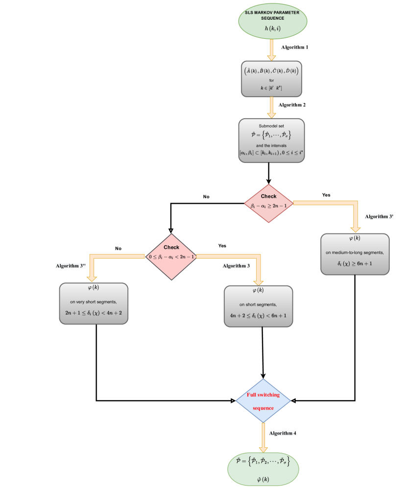
Figure 1: A meta-algorithm for the SLS realization from Markov parameters sequence.

Theorem 8.1.

Consider (2)–(4) with the noisy Markov parameters in (38). Assume that $\chi$, and $\mathcal{P}$ satisfy Assumptions 3.1–3.2, 4.1, 5.1, 6.1, and 7.1. If Assumption 4.2 holds, then the meta-algorithm recovers ${\mathcal{P}}$ and $\chi$ as $\varepsilon\rightarrow 0$. Suppose that the first part of Assumption 4.2 holds and $\varphi$ satisfies a mixing condition. If each segment in $\chi$ satisfies a dwell requirement in one of Theorems 5.1, 6.1, and 6.3, then the meta-algorithm recovers ${\mathcal{P}}$ and $\chi$ as $\varepsilon\rightarrow 0$.

In all algorithms we developed so far, observability and controllability concepts have played a foundational role. We have assumed that the discrete states have a common Macmillan degree. When this assumption is dropped, identifiability, controllability, and observability for the MIMO-SLS models become much harder to analyze. For example, identifiability of an SLS does not imply identifiability of its submodels [62]. Pivotal role played by observability in the estimation/realization of the SLSs has been noted early in hybrid system literature [30]. The observability part of Lemma 3.1 appeared as Theorem 2 in [25]. Extension of the Ho-Kalman realization theory for the LPV state-space models was reported in [48].

This paper did not address the issue of estimating Markov parameters from input-output data. The reasons are twofold. First, the realization problem for SLSs is interesting in its own [21, 22, 63, 64]. See also the references therein. An equally important subject in SLSs is model order reduction. We refer to recent works [65, 66, 67]. Second, we decoupled identification and realization problems and treated the latter in great detail in this paper though both can be treated in a unified manner. This approach has several merits. Identification of an SLS is normally conducted in two stages: estimation of the discrete states and detection of the switches, with the order being interchangeable. The realization problem solved in this paper recovers the switching sequence in addition to the discrete states. The switching sequence is an arbitrary time-varying signal subject to mild restrictions in contrast to existing works in hybrid systems literature. By lifting the issue of estimating the switching sequence to the realization stage, attention is directed to estimating the Markov parameters in parsimonious models.

One approach for estimating Markov parameters is to use multiple trajectories when it is possible [28, 55, 56]. But, this approach has limited applications to system identification. Markov parameter estimation problem is not tractable for generic LTV systems due to the curse of dimensionality, unless further system assumptions such as slowly varying or smooth, mode switching with long waiting times, etc. are made. In [14], switched ARX models were identified by a kernel based estimation method. This method encompasses the parameter estimation and the switch detection stages by solving an optimization problem. Recent work [35] used deadbeat observers to transform state-space identification problem into an SARX identification problem. This transformation generates parsimonious models by packing infinite strings of Markov parameters into finite sequences. In principle, any of these methods can be used to estimate Markov parameters. Work is under progress for direct estimation of the Markov parameters from input-output data.

9 Numerical example

Consider the following MIMO–SLS state-space model adapted from [34]

$${A_{1}} = \left[{\begin{array}[]{*{20}{c}}{0.15}&{0.40}&{-0.65}\\ {-0.75}&{0.1}&{-0.35}\\ {0.20}&{0.70}&{0.20}\end{array}}\right],\;\;{B_{1}}=\left[{\begin{array}[]{*{20}{c}}{-0.20}&{0.45}\\ {-0.06}&0\\ {0.22}&0\end{array}}\right]$$

$${C_{1}} = \left[{\begin{array}[]{*{20}{c}}0&{0.40}&{0.45}\\ {-1}&{-0.60}&{0.90}\end{array}}\right],\;\;{D_{1}}=\left[{\begin{array}[]{*{20}{c}}0&{-0.35}\\ {-1.70}&{-0.25}\end{array}}\right]$$

$${A_{2}} = \left[{\begin{array}[]{*{20}{c}}{0.27}&{0.24}&{-0.55}\\ {0.24}&{0.65}&{0.30}\\ {-0.55}&{0.30}&{0.27}\end{array}}\right],\;\;{B_{2}}=\left[{\begin{array}[]{*{20}{c}}{-0.55}&0\\ {-1.40}&1\\ {0.05}&{-0.72}\end{array}}\right]$$

$${C_{2}} = \left[{\begin{array}[]{*{20}{c}}{0.70}&1&{-0.27}\\ {-0.35}&0&{-1.10}\end{array}}\right],\;\;{D_{2}}=\left[{\begin{array}[]{*{20}{c}}{2.15}&{0.25}\\ 0&{-0.36}\end{array}}\right]$$

$${A_{3}} = \left[{\begin{array}[]{*{20}{c}}{0.45}&{0.02}&{0.42}\\ {-0.17}&{0.53}&{0.20}\\ {0.38}&{0.26}&0\end{array}}\right],{B_{3}}=\left[{\begin{array}[]{*{20}{c}}0&{0.15}\\ {0.27}&{-0.46}\\ {0.07}&{0.54}\end{array}}\right],\;\;$$

$${C_{3}} = \left[{\begin{array}[]{*{20}{c}}0&{0.60}&{0.28}\\ 0&{0.86}&{0.45}\end{array}}\right],\;\;{D_{3}}=\left[{\begin{array}[]{*{20}{c}}0&{-0.90}\\ 0&{0.85}\end{array}}\right]$$

where the problem of identifying a state-space SLS model for the case when the continuous state is known was treated. In the sequel, we address the problem of discrete state estimation given an exact sequence of Markov parameters.

9.1 SLS estimation in a noiseless setup

We first deal with the estimation of the discrete-states.

9.1.1 Discrete state estimation

A switching sequence that conforms with Assumption 4.2 in all but few segments was generated via sampling from a random uniform distribution. It is shown in Figure 2 where the red dots represent the switches. The discrete state estimation was accomplished via Algorithm 2. As inputs to the algorithm, we selected $\epsilon_{\mathbb{Z}}=10^{-4}$, $\nu=6$, and estimated the state-space quadruples $\hat{\mathcal{P}}_{k}$ over the time range $k^{\prime}\leq k\leq k^{\prime\prime}$ from Algorithm 1. The dbscan command in MATLAB was implemented by selecting epsilon=$10^{-5}$ as a threshold value for the neighborhood search radius and minpts=1 for the minimum number of neighbors. As an entry to dbscan, we supplied ${\mathcal{M}}(\hat{A}(\gamma_{i}))$ as the clustering feature where $\gamma_{i}$ is the midpoint of the targeted intervals which satisfy $\beta_{i}-\alpha_{i}\geq 6n$. Let $\mathcal{I}=\left\{{i:\;{\beta_{i}}-{\alpha_{i}}\geq vn}\right\}$ denote the set of indices satisfying this constraint. Figure 3(a) shows the clustering result over ${\mathcal{M}}(\hat{A}(\gamma_{i}))$, $i\in\mathcal{I}$. As anticipated, $\sigma$ is correctly estimated, i.e., $\hat{\sigma}=3$. Using clusters, we now determine the set of submodel estimates $\hat{\cal P}_{j}$, $j\in\mathbb{S}$. Notice that not all segments satisfy $\beta_{i}-\alpha_{i}\geq\nu n$, yet recovery is perfect.

To assess the fitting capability of the estimates, the submodel estimates’ eigenvalues were compared to the true ones as shown in Figure 3(b). Observe the exact matches to the true eigenvalues.

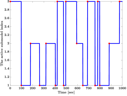
Figure 2: The switching sequence in the example.

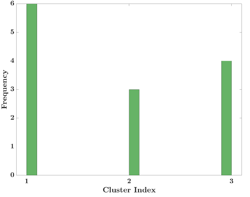
(a) The histogram of clusters over the $1$-d feature space $\left\{{{\cal M}(\hat{A}({\gamma_{i}})),i\in\mathcal{I}}\right\}$.

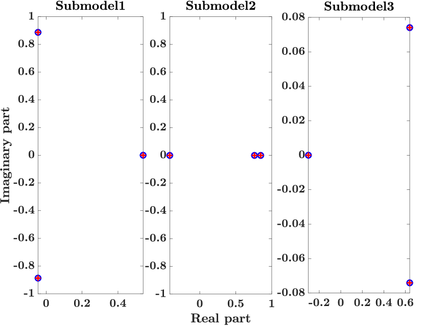
(b) The estimated ’$\circ$’ and the true ’+’ submodel eigenvalues in a noiseless setup.

Figure 3: The discrete state estimation via Algorithm 2 (see Appendix).

9.1.2 Switching sequence estimation

Now we address the issue of switching sequence estimation assuming that the submodel set was estimated in the previous stage. This could be achieved via Algorithm $3^{\prime}$ solely if our SLS has a minimum dwell time of at least $6n+1$, i.e, ${\delta_{*}}\left(\chi\right)\geq 6n+1$. On the other hand, Algorithm 3 can be used if $\delta_{*}\left(\chi\right)\geq 4n+2$. Lastly, if there exist very short segments with a minimum dwell time of at least ${\delta_{*}}\left(\chi\right)\geq 2n+1$, we use Algorithm $3^{\prime\prime}$. We call a segment $[k_{i},k_{i+1})$ satisfying $\delta_{i}(\chi)\geq 6n+1$ ’medium-to-long’, a segment $[k_{i},k_{i+1})$ with $6n+1>\delta_{i}(\chi)\geq 4n+2$ ’short’, and lastly a segment $[k_{i},k_{i+1})$ satisfying $4n+2>\delta_{i}(\chi)\geq 2n+1$ ’very short’. Algorithms $(3^{\prime},3,3^{\prime\prime})$ estimate the medium-to-long, the short, and the very short segments, respectively. To show their working mechanisms, we generated a switching sequence containing segments of the three types. Different type segments were marked with distinctive colors for better discernibility: medium-to-long ’blue’, short ’brown’, and very short ’black’. The switching sequence generated is shown in Figure 4(a). In Figure 4(b), the segments in $\chi$ are classified according to their types.

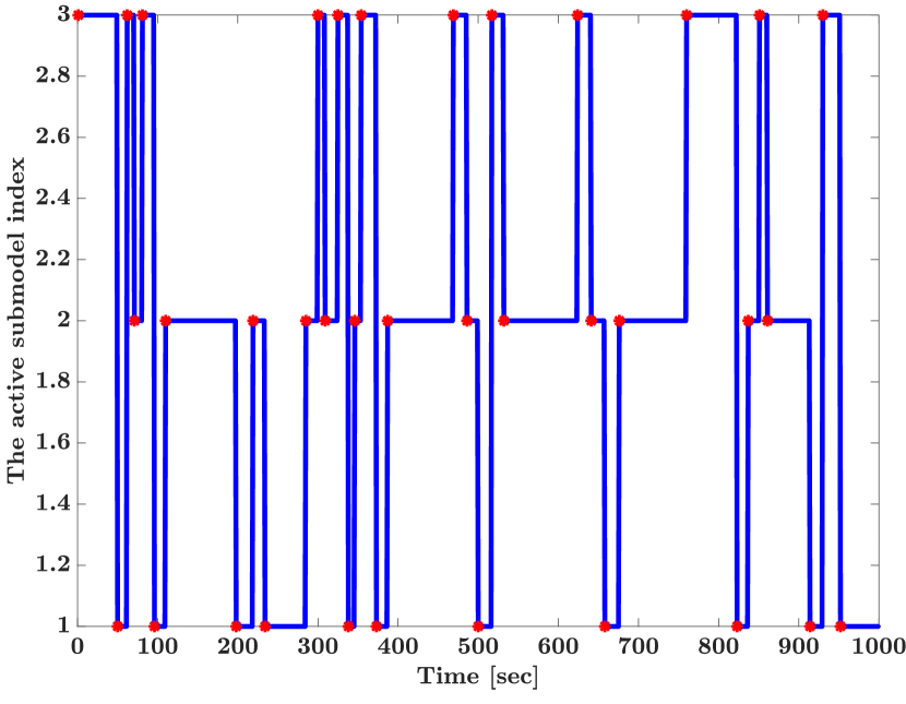
(a) The switching sequence.

(b) The medium-to-long ’blue’, the short ’brown’, and the very short ’black’ segments in the switching sequence of Figure 4(a).

Figure 4: The switching sequence generated in Section 9.1.2.

We start by estimating the submodels, and this is accomplished via Algorithm 2 with $\nu=6$. Next, we sequentially run the switch detection algorithms. We first try Algorithm $3^{\prime}$ over the medium-to-long segments, but it fails to estimate the switching sequence at some points in the short and the very short segments. This explains why a large set of points are not yet attributed to any of the submodels as shown in Figure 5(a). These points were put in Cluster 0 to distinguish them from the points in the segments which have already been attributed a correct submodel index. The red dots are the switches as before. Next, we try Algorithm $3$ to estimate the switching sequence over the short segments, but it fails at some points in the very short segments. The switching sequence estimate is shown in Figure 5(b). Finally, we run Algorithm $3^{\prime\prime}$ to estimate the rest of the switching sequence, i.e., over the very short segments. The final switching sequence estimate and its zoomed image are shown in Figure 5(c) and Figure 7. It is an exact match to the true one. As a final remark, note that Algorithm 3’ operates on the intervals satisfying $\beta_{i}-\alpha_{i}\geq\nu n$. This condition was used in Algorithm 2 to estimate the discrete states.

(a) The medium-to-long segment estimation via Algorithm $3^{\prime}$.

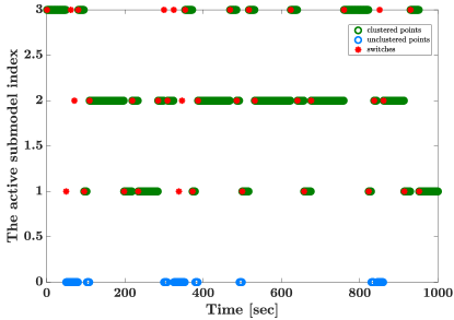
(b) The short segment estimation via Algorithm 3.

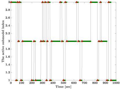
(c) The final switching sequence estimate ’$\circ$’, the true switching sequence ’-’, and the switches ’$\triangle$’.

Figure 5: The switching sequence estimation via Algorithms $(3^{\prime},3,3^{\prime\prime})$ in order.

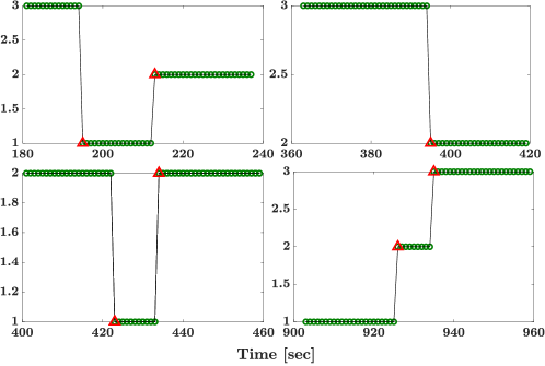
Figure 6: The true ’$\circ$’ and the estimated ’-’ switching sequences zoomed from Figure 5(c).

9.1.3 Basis transform for the discrete states

This subsubsection is concerned with performing the necessary discrete state transformations to render the SLS model usable for predicting output given an input signal. To perform that, one needs the estimated sub-models from Algorithm 2 and the estimated switching sequence from Algorithms $(3,3^{\prime},3^{\prime\prime})$. Having that, we employ Algorithm 4 to obtain ${\Pi_{j}}={T_{j}}T_{1}^{-1}$ for $j=2,3$. They were calculated as follows

$${\Pi_{2}}=\left[{\begin{array}[]{*{20}{c}}{{\rm{-0}}.{\rm{4549}}}&{{\rm{0}}.{\rm{0311}}}&{{\rm{0}}.{\rm{1299}}}\\ {{\rm{-0}}.{\rm{0140}}}&{{\rm{0}}.{\rm{5774}}}&{{\rm{-0}}.{\rm{2281}}}\\ {{\rm{-0}}.{\rm{4472}}}&{{\rm{-0}}.{\rm{3224}}}&{{\rm{-0}}.{\rm{8538}}}\end{array}}\right],$$

$${\Pi_{3}}=\left[{\begin{array}[]{*{20}{c}}{{\rm{-0}}.{\rm{4595}}}&{{\rm{0}}.{\rm{1516}}}&{{\rm{0}}.{\rm{9003}}}\\ {{\rm{-0}}.{\rm{0115}}}&{{\rm{-0}}.{\rm{1930}}}&{{\rm{0}}.{\rm{2244}}}\\ {{\rm{-0}}.{\rm{2481}}}&{{\rm{-0}}.{\rm{1360}}}&{{\rm{-0}}.{\rm{0860}}}\end{array}}\right].$$

After that, we apply ${\Pi_{j}}$ to $\mathcal{\hat{P}}$ to put all the submodels in a common state basis. In particular, we apply ${\Pi_{2}}$ to ${{\hat{\cal P}}_{2}}$ to render it in a common state basis as of that corresponding ${{\hat{\cal P}}_{1}}$. In a similar manner, ${\Pi_{3}}$ is applied to ${{\hat{\cal P}}_{3}}$ which transforms its basis to that of ${{\hat{\cal P}}_{1}}$. To demonstrate the effectiveness of this approach, we generated an input signal as a sum of harmonics, and we simulated its output through the SLS model. We did that both for the original SLS and the estimated one, and we inspected the match between the two. In generating the output signal we assumed that there were no switches occurring before $k^{\prime}$ and after $k^{\prime\prime}$, hence we extended $\hat{\varphi}\left(k\right)$ to $1$ and $N$. Both the true and the modeled SLSs were started at rest, i.e., the initial state was taken to be $x_{0}=[0\;\;0\;\;0]^{T}$. Figure 7 displays the true output signals and the estimation errors side by side.

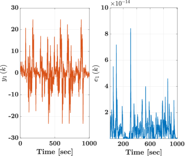
(a) True Output 1 (left) and the estimation error (right).

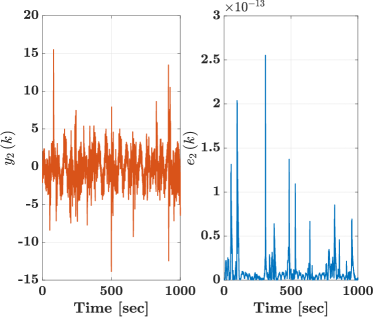
(b) True Output 2 (left) and the estimation error (right).

Figure 7: The outputs and the estimation errors.

To assess the fidelity of these estimates, we introduce the variance-accounted-for criterion defined by

$$VAF=\left({1-\frac{{{\rm{var}}\left({y\left(k\right)-\hat{y}\left(k\right)}\right)}}{{{\rm{var}}\left({y\left(k\right)}\right)}}}\right)\times 100\%.$$ (157)

We calculated (157) for both outputs. For Output 1, we got VAF=99.99$\%$ and for Output 2, VAF=99.99$\%$ indicating perfect match between the two. This perfect match resulted from the agreement between the pairs true switching sequence-Markov parameter set and their estimates since the I/O map explicitly depends on them.

9.2 SLS recovery from noisy Markov parameters measurements

We now study SLS recovery in a noisy setup. The same SLS model as in the noiseless case was adopted here. Table I lists the smallest nonzero singular values in the noiseless Hankel matrices of the submodels, which according to [45] determine how robustly a realization algorithm could retrieve a particular discrete state. It is clear from the table that Submodels 1 and 2 can be learned better than Submodel 3 when the exact Markov parameters pertaining to these submodels are perturbed with the same noise level.

Table 1: The smallest nonzero singular values in the Hankel matrices of the individual submodels.

Submodel	$\mathcal{P}_{1}$	$\mathcal{P}_{2}$	$\mathcal{P}_{3}$
${\sigma_{\min}}$	0.4063	0.3560	0.0180

We generated a switching sequence by sampling from a uniform distribution. Instead of using the exact Markov parameters, we contaminated them via an additive white noise. From the noisy doubly indexed Markov parameters, the SLS identification was conducted similarly to the previous case. Algorithm 2 recovered the submodels. These submodels were exploited to retrieve the switching sequence by running Algorithms $(3,3^{\prime},3^{\prime\prime})$ depending on the type of segment considered. Algorithm 4 transformed the discrete states estimated in a precedent stage to a common state basis so that the output prediction could be conducted harmlessly. This could be as well inspected by checking that the true Markov parameters and the estimated ones are identical through the entire time interval. The individual steps are summarized in the flowchart of Figure 1. Figure 8 plots the feature used for clustering defined in (71) together with the switching sequence for one noise realization with signal-to-noise ratio (SNR) 40dB. Note the gross error in the last segment in agreement with Table I, that is, the realization algorithm performs poorly when it tries to learn Submodel 3. The estimated SLS eigenvalues shown in Figure 9 highly mismatch the eigenvalues of Submodel 3.

(a) The switching sequence in Section 9.2.

(b) ${\cal M}({\hat{A}}(k))$ (blue) and ${\mathcal{M}}(A(k))$ (red) for one noise realization at SNR=40dB.

Figure 8: The switching sequence and the feature used for clustering in (71).

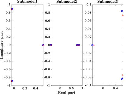
Figure 9: The eigenvalue estimates for one noise realization at SNR=40dB: the true ’+’and the estimates ’$\circ$’.

To study robustness of the meta-algorithm to noise, we calculated the mismatch error in estimating the true Hankel matrix in (9) defined pointwise in time by

$${\varepsilon_{\mathcal{H}}}\left(k\right)={\left\|{{\mathcal{H}_{2n+1,2n}}\left(k\right)-{{\hat{\mathcal{H}}}_{2n+1,2n}}\left(k\right)}\right\|_{F}},\quad\forall k\in[k^{\prime}\;\;k^{\prime\prime}]$$ (158)

where ${{{\hat{\mathcal{H}}}_{2n+1,2n}}\left(k\right)}$ is the Hankel matrix estimate. Since the SLS realization problem involves both $\varphi$ and $\mathcal{P}$, we selected a criterion reflecting both through Markov parameters. Alternatively, we could have conducted output predictions to prescribed inputs. Figure 10 displays the mismatch error (158) as a function of time for a range of SNRs. The mismatch error is flat over the segments with the exception of the switches where the changes in the discrete states are abrupt. As SNR is decreased, the mismatch error increases rapidly.

(a) SNR=45dB.

(b) SNR=40dB.

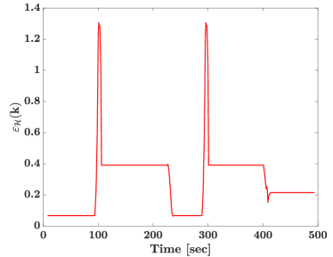
(c) SNR=35dB.

Figure 10: The mismatch error (158) at different SNRs.

9.3 Realization from input-output data

In this subsection we demonstrate how our meta-algorithm could be incorporated in a complete system identification package that estimates an SLS starting from the input-output measurements rather than the Markov parameters. To achieve this goal, we append our meta-algorithm to an identification algorithm proposed in [35] to form a two-stage algorithm. The algorithm in [35] is a standalone algorithm which can be used to fully estimate an SLS in the state-space form from the input-output data. It can also be used to estimate the Markov parameters by solving a sparse optimization problem. We emphasize that this algorithm successfully retrieves the Markov parameters from a single trajectory, unlike the earlier works [55, 56, 28] where multiple trajectories are assumed to be available.

Solution of sparse optimization problem essentially grants us a finite set of observer Markov parameters which encodes entire knowledge of the system dynamics. From observer parameters, one can retrieve infinite strings of the Markov parameters. Without going into technical details, it suffices to say that conditions on the input-output data, the dwell times, persistence of excitation on the inputs, and some identifiability criteria permit successful recovery of the Markov parameters. The meta-algorithm of this paper complements this scheme. Let us consider the SLS model

$${A_{1}} = \left[{\begin{array}[]{*{20}{c}}0&{0.8}\\ {-0.8}&{0.5}\end{array}}\right],\;\;{B_{1}}=\left[{\begin{array}[]{*{20}{r}}{1.4}\\ {-2}\end{array}}\right],\;\;C_{1}=-\left[{1\;\;1.5}\right],\;\;{D_{1}}=1$$

$${A_{2}} = \left[{\begin{array}[]{*{20}{c}}{-0.9}&{-1.25}\\ {1.8}&{1.5}\end{array}}\right],\;\;{B_{2}}=\left[{\begin{array}[]{*{20}{r}}{-1}\\ {0.5}\end{array}}\right],\;\;C_{2}=\left[{-1\;\;1}\right],\;\;{D_{2}}=-1.5;$$

$${A_{3}} = \left[{\begin{array}[]{*{20}{c}}{0.8}&0\\ 0&{-0.3}\end{array}}\right],\;\;{B_{3}}=\left[{\begin{array}[]{*{20}{r}}1\\ 2\end{array}}\right],\;\;C_{3}=\left[{2\;\;3}\right],\;\;{D_{3}}=2.$$

We generated a switching sequence of length $N=1,000$ by sampling from a uniform distribution. The SLS model was excited with a multi-sine input starting from the initial condition $x(0)=(0\;\;0)^{T}$. Running Algorithm 6 in [35] by using the CVX package [68] with the observer order $\tau=2n$, we get the observer Markov parameter estimates $h_{\rm o}(k,k-\ell)$ for $2n<k\leq N-2n$ and $0\leq\ell<2n$. Let us call Algorithm 1 in [35] Algorithm 1^′ to avoid confusion with Algorithm 1 in this paper. Algorithm 1^′ driven by the observer Markov parameters returns $h(k,k-\ell)$ for $0\leq\ell\leq k$ and $2n<k\leq N-2n$. Algorithm 1 relies only on the first $4n+1$ Markov parameters. Thus, running Algorithm 1^′ we get as many Markov parameter estimates as we want. Having estimated the Markov parameters, we run the meta-algorithm. We will perform a Monte-Carlo simulation study for $100$ noise realizations.

The eigenvalues estimated by this two-stage scheme are plotted in Figure 11. The average case performance will be assessed by first computing the relative errors $\|M_{j}-\hat{M}_{j}\|_{F}/\|M_{j}\|_{F}$, $j\in\mathbb{S}$ where ${\hat{\cal P}_{j}}=({{\hat{A}}_{j}},{{\hat{B}}_{j}},{{\hat{C}}_{j}},{{\hat{D}}_{j}})$ and

$${{\hat{M}}_{j}}=\left[{\begin{array}[]{*{20}{c}}{{{\hat{A}}_{j}}}&{{{\hat{B}}_{j}}}\\ {{{\hat{C}}_{j}}}&{{{\hat{D}}_{j}}}\end{array}}\right],$$

summing over $\mathbb{S}$, and averaging over $100$ realizations. The result is denoted by $\delta_{\mathcal{P}}$. In Table 2, $\delta_{\cal P}$ is displayed for $20,30$, and $40$dB SNRs. In the same table we compared the two stage scheme reported here to the algorithm in [34], which assumes the availability of state measurements and proceeds by solving a sparse SARX regression optimization problem. However, the availability of the state measurements is a stringent assumption in practice.

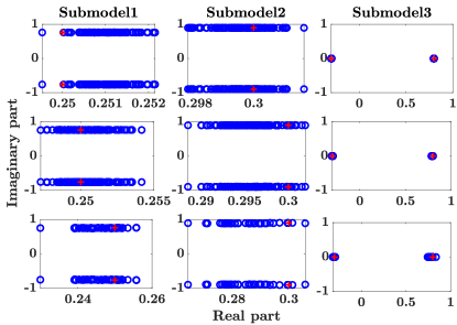
Figure 11: The true ’+’ and the estimated ’$\circ$’ eigenvalues for $100$ noise realizations at $20,30$, and $40$dB SNRs (top-to-bottom).

Table 2: $\delta_{\cal P}$ calculated over the 100 noise realizations.

Schemes	$\delta_{\cal P}$
SNR (dB)	40dB	30dB	20dB
Proposed	0.0169	0.0297	0.0839
[34]	0.0104	0.0404	0.1581

A measure of fit for the switching sequence estimates is the percentage of correctly classified points. It is called FIT_φ and calculated by the formula

$${\rm FI}{\rm T}_{\varphi}=\left(1-\frac{1}{N}\sum\limits_{k=1}^{N}sign\left|\hat{\varphi}(k)-\varphi(k)\right|\right)\times 100\%.$$ (162)

Figure 12 plots the histogram of FIT_φ over $100$ noise realizations at SNR=$30$dB for both our approach and the scheme in [34]. From Table 2 and Figure 12 we see that the two-stage scheme outperforms the algorithm in [34] and have an edge in the sense that it operates under mild assumptions.

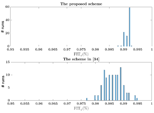
Figure 12: The histogram of ${\rm{FI}}{{\rm{T}}_{\varphi}}$ over $100$ noise realizations at $SNR=30$dB.

9.4 Realization of randomly generated SLSs

In this subsection, we examine the performance of the meta-algorithm in estimating randomly generated SLSs. The discrete states were sampled from a normal distribution. The switching sequences were generated by sampling from a uniform distribution similarly to the previous subsections. The SLSs and the switching sequences satisfy Assumptions 3.1–3.2, 4.1, 5.1, 6.1, and 7.1. Randomly generated SLSs were corrupted by noise to achieve a certain SNR prior to carrying out identification. We then generated the Markov parameters to drive the meta-algorithm. In this study, we considered SISO-SLSs with $n=2$ and $\sigma=3$. We picked $N=650$ for Monte-Carlo simulations and assessed the performance of our algorithm using first $\delta_{\cal P}$ and FIT_φ. The results in Table 3 were obtained by first estimating an SLS and $\varphi$ for each run and averaging the sum of the relative errors and ${\rm FIT}_{\varphi}$ over 50 runs. For each run, we picked a random SLS and a random noise realization. We repeat calculations for a range of SNRs to fill the table. As another measure of performance, for each run next we calculated the RMS value of (158) over $k$ and averaged it over $50$ runs. The results are plotted in Figure 13 as a function of SNR levels.

Table 3: The average performance of the meta-algorithm in estimating randomly generated SLSs.

Errors	$\delta_{\cal P}$				FITφ ($\%$)
SNR (dB)	50dB	40dB	30dB	20dB	50dB	40dB	30dB	20dB
Average Values	0.0110	0.0423	0.1818	0.7651	100	99.98	98.20	94.54

Figure 13: The average RMS of the error in (158) calculated over $50$ runs at different SNRs.

10 Conclusions

This paper laid forward a four-stage algorithm for the realization of MIMO-SLSs from Markov parameters. Its first stage recovers an LTV realization that is topologically equivalent to the SLS under mild system and dwell time assumptions. Since topological equivalence does not guarantee similarity to the discrete states on any segment, it was necessary to apply forward/backward corrections point-wise in time to the LTV realization, to reveal the segments. This process established a time-varying similarity to the discrete states. Next, the stationary point set on which the LTV realization has an LTI pulse response were sought. This search was effected by a clustering algorithm using a feaure space that is invariant to similarity transformations. Combination of these schemes formed Stage 2 of the realization algorithm. In this stage, the discrete state estimates similar to the true ones were extracted from the LTV realization under some dwell time and identifiability conditions. In the third stage, the switching sequence was estimated by three schemes, complementing each other. The first scheme operates on the forward/backward corrections and estimates the switching sequence over short segments. The second scheme is based on matching the estimated and the true Markov parameters for LTV systems and it can be applied to medium-to-long segments. The third scheme is also based on matching the Markov parameters, but for LTI systems only via Hankel matrix factorization. It can be applied to segments of even shorter length which cannot be handled by the first two schemes. The schemes are applied in the order second-to-first-to-third. The issue of discrete states residing in different state bases were resolved by applying a basis correction in Stage 4; this equips the retrieved SLS with the potential to conduct output predictions.

The success of the various schemes in the realization algorithm put us face to face with the compulsion to impose several restrictions on the discrete state set and their dwell times; nonetheless, all that can be said is that they are mild in nature. The involvement of the observability and controllability matrices in the schemes presented so far was quite noticeable, as noted in several other related works in the literature on SLS identification and realization. Future work will focus on developing an identification algorithm to estimate the Markov parameters from input-output measurements of a single trajectory.

Appendix: Pseudo codes for the algorithms

Algorithm 1. LTV realization from Markov parameters

Set $q=2n+1$ and $r=2n$.

Inputs: Markov parameters $h(k+i,k-j)$ for $0\leq i<q$,

$1\leq j\leq r$, $k\in[k^{\prime}\;\;k^{\prime\prime}]$

while $k\in[k^{\prime}\;\;k^{\prime\prime}]$

1: Compute ${\mathcal{H}}_{q,r}(k)$ and ${\mathcal{H}}_{q,r}(k+1)$ from (33)–(37)

2: Compute the SVDs in (LABEL:svdHqr)

3: Compute the extended observability/controllability

matrices estimates in (25-26)

4: Estimate $\hat{A}(k)$, $\hat{C}(k)$, $\hat{B}(k)$ from (27) and (31),

and $\hat{D}(k)=h(k,k)$

5: $k\leftarrow k+1$

end while

Outputs: $\hat{\mathcal{P}}(k)=(\hat{A}(k),\hat{B}(k),\hat{C}(k),\hat{D}(k))$, $\forall k\in\mathcal{K}$.

Algorithm 2. Discrete state estimation

Inputs: Markov parameters $h(k+i,k-j)$ for $0\leq i<2n+1$,

$1\leq j\leq 2n$, $k\in[k^{\prime}\;\;k^{\prime\prime}]$, a small $\varepsilon_{\mathbb{Z}}>0$, and $\nu>5$.

1: Compute $\delta_{\mathcal{H}}(k)$, for all $k\in[k^{\prime}\;\;k^{\prime\prime}]$ from (69)

2: Initialize $\mathbb{Z}_{{\mathcal{H}},\varepsilon_{\mathbb{Z}}}=\phi$

3: while $k\in[k^{\prime}\;\;k^{\prime\prime}]$

if $\left\|\delta_{\mathcal{H}}(k)\right\|_{F}\leq\varepsilon_{\mathbb{Z}}$

$\mathbb{Z}_{{\mathcal{H}},\varepsilon_{\mathbb{Z}}}=\mathbb{Z}_{{\mathcal{H}},\varepsilon_{\mathbb{Z}}}\cup\{k\}$

end if

$k\leftarrow k+1$

end while

4: Identify maximal disjoint intervals $[\alpha_{i},\beta_{i}]\subset\mathbb{Z}_{{\mathcal{H}},\varepsilon_{\mathbb{Z}}}$, $\beta_{i}-\alpha_{i}\geq\nu n$

5: Retrieve $\hat{A}(\gamma_{i})$, $\gamma_{i}=(\alpha_{i}+\beta_{i})/2$ from the output Algorithm 1 .

6: Compute ${\mathcal{M}}(\hat{A}(\gamma))$

7: Estimate $\mathcal{P}$ by running the clustering algorithm in [59] over $\gamma$

and re-clustering if necessary

Outputs: $\hat{\cal P}_{j}$, $j\in\mathbb{S}$ and the intervals in Step 4 containing them.

Algorithm 3. Switch detection based on corrections Inputs: $S_{i}=[\alpha_{i},\beta_{i}]$, $0\leq i\leq i^{*}$; $h(k+i,k-j)$, $0\leq i<2n+1$,

$1\leq j\leq 2n$, $k\in[k^{\prime}\;\;k^{\prime\prime}]$

Run the following loop:

for $0\leq i\leq i^{*}$

if ($i==0$ and $\delta_{0}(\chi)\geq 6n+2$) or ($i\neq 0$, $i\neq i^{*}$, and $\delta_{i}(\chi)\geq 4n+2$)

Initialize $k=\beta_{i}-2n$

while $|{\mathcal{M}}(\hat{\mathcal{V}}_{2n+1}(k))-n|<\varepsilon$

k=k+1

end while

$k_{i+1}=k+2n+1$

end if

if ($i==i^{*}$ and $\delta_{i^{*}}(\chi)>8n$) or ($i\neq 0$, $i\neq i^{*}$, and $\delta_{i}(\chi)\geq 4n+2$)

Initialize $k=\alpha_{i}+2n-1$

while $|{\mathcal{M}}(\hat{\mathcal{W}}_{2n}(k))-n|<\varepsilon$

k=k-1

end while

$k_{i}=k-2n+1$

end if

end for

Outputs: $\varphi(k)$ on segments satisfying ${\delta_{i}}\left(\chi\right)\geq 4n+2$

Algorithm 3′. Switch detection from Markov parameters Inputs: $\hat{\mathcal{P}}(\gamma_{i})$, $\gamma_{i}=(\alpha_{i}+\beta_{i})/2$, $S_{i}=[\alpha_{i},\beta_{i}]$, $0\leq i\leq i^{*}$;

$h(k+i,k-j)$, $0\leq i\leq 2n$, $1\leq j\leq 2n$, $k\in[k^{\prime}\;\;k^{\prime\prime}]$, $\varepsilon>0$

Run the following loop:

for $0\leq i\leq i^{*}$

if ($i==0$ and $\delta_{0}(\chi)\geq 8n+1$) or ($i\neq 0$, $i\neq i^{*}$, and $\delta_{i}\geq 6n+1$)

Initialize $\ell=\beta_{i}-1$, $\check{C}=\hat{C}(\gamma_{i})$, $\check{D}=\hat{D}(\gamma_{i})$

while $\|\check{C}-\hat{C}(\gamma_{i})\|_{F}+\|\check{D}-\hat{D}(\gamma_{i})\|_{F}<\varepsilon$

$\ell=\ell+1$

$\check{C}={\mathcal{H}}_{1,2n}(\ell)\hat{\mathcal{R}}_{2n}^{\dagger}(\ell-1)$, $\check{D}=\hat{D}(\ell)$

end while

Set $k_{i+1}=\ell$

end if

if ($i==i^{*}$ and $\delta_{0}(\chi)\geq 10n$) or ($i\neq 0$, $i\neq i^{*}$, and $\delta_{i}\geq 6n+1$)

Initialize $\ell=\alpha_{i}+1$, $\check{B}=\hat{B}(\gamma_{i})$, $\check{D}=\hat{D}(\gamma_{i})$

while $\|\check{B}-\hat{B}(\gamma_{i})\|_{F}+\|\check{D}-\hat{D}(\gamma_{i})\|_{F}<\varepsilon$

$\ell=\ell-1$

$\check{B}=\hat{\mathcal{O}}_{2n}^{\dagger}(\ell+1){\mathcal{H}}_{2n,1}(\ell+1)$, $\check{D}=\hat{D}(\ell)$

end while

Set $k_{i-1}=\ell+1$

end if

end for

Outputs: $\varphi(k)$ on segments satisfying ${\delta_{i}}\left(\chi\right)\geq 6n+1$

Algorithm 3′′. Switch detection on short intervals Inputs: $\hat{\mathcal{P}}$, one switch from each segment, Markov parameters, and $\varepsilon>0$

Run the following loop:

for $1\leq i<i^{*}$

while $\delta_{i}(\chi)>2n$ and $k_{i}$ is known ’forward estimation’

1: Compute $\hat{\mathcal{P}}(\gamma_{i})$ from (140) and let $\varphi(k)=\varphi(\gamma_{i})$ on $[k_{i},k_{i}+2n]$

2: Estimate $k_{i+1}$ and extend $\hat{\mathcal{P}}(\gamma_{i})$ to $(k_{i}+2n,k_{i+1})$

by forward updating in Algorithm 3′

end while

while $\delta_{i-1}(\chi)>2n$ and $k_{i}$ is known ’backward estimation’

1: Compute $\hat{\mathcal{P}}(\gamma_{i-1})$ from (141) and let $\varphi(k)=\varphi(\gamma_{i-1})$ on $[k_{i}-2n,k_{i})$

3: Estimate $k_{i-1}$ and extend $\hat{\mathcal{P}}(\gamma_{i-1})$ to $[k_{i-1},k_{i}-2n)$

by backward updating in Algorithm 3′

end while

end for

if $\delta_{i^{*}}(\chi)\geq 6n$

‘$k_{i^{*}}$ is known’ $\Rightarrow$ ’forward estimation from $k_{i^{*}}$’

‘$k_{i^{*}}$ is not known’ $\Rightarrow$ ’backward estimation from $k^{\prime\prime}+1$’

end if

if $\delta_{0}(\chi)>4n$

‘$k_{1}$ is known’ $\Rightarrow$ ’backward estimation from $k_{1}$’

‘$k_{1}$ is not known’ $\Rightarrow$ ’forward estimation from $k^{\prime}$’

end if

Outputs: $\varphi(k)$ on segments satisfying ${\delta_{i}}\left(\chi\right)\geq 2n+1$

Algorithm 4. Basis transformation for the discrete states Inputs: Markov parameters, $\hat{\mathcal{P}}$ (ordered), and $\varphi$ 1: Estimate $\Pi_{j}=T_{j}T_{1}^{-1}$ for $j=2,\cdots,\sigma$ from (144)–(146) and (147)–(LABEL:esek4) with $j$ and $1$ plugged in places of $j_{2}$ and $j_{1}$ by choosing suitable paths and inversions if needed 2: Transform $\hat{\mathcal{P}}_{j}$ to $\check{\mathcal{P}}_{j}$ using $\Pi_{j}$ as the similarity transformations for $j=2,\cdots,\sigma$. Outputs: $\hat{\mathcal{P}}_{1}$ and $\check{\mathcal{P}}_{j}$, $j=2,\cdots,\sigma$.

References

- [1] R. Rui, T. Ardeshiri, and A. Bazanella, “Identification of piecewise affine state-space models via expectation maximization,” in: Proceedings of the IEEE Conference on Computer Aided Control System Design, Buenos Aires, Argentina, pages 1066–1071, September 2016.
- [2] S. Paoletti, A. L. Juloski, G. Ferrari-Trecate, and R. Vidal, “Identification of hybrid systems a tutorial,” European Journal of Control, vol. 13, no. 2-3, pp. 242–260, 2007.
- [3] R. Vidal, “Recursive identification of switched ARX systems,” Automatica, vol. 44, no. 9, pp. 2274–2287, 2008.
- [4] N. Ozay, M. Sznaier, C. M. Lagoa, and O. I. Camps, “A sparsification approach to set membership identification of switched affine systems,” IEEE Transactions on Automatic Control, vol. 57, no. 3, pp. 634–648, 2011.
- [5] N. Ozay, C. Lagoa, and M. Sznaier, “Set membership identification of switched linear systems with known number of subsystems,” Automatica, vol. 51, pp. 180–191, 2015.
- [6] X. Jin and B. Huang, “Robust identification of piecewise/switching autoregressive exogenous process,” AIChE Journal, vol. 56, no. 7, pp. 1829–1844, 2010.
- [7] R. Murray-Smith, “Modelling human control behaviour with context-dependent Markov-switching multiple models,” IFAC Proceedings Volumes, vol. 31, no. 26, pages 461–466, 1998.
- [8] A. Mestre, Hybrid subspace identification: an application to HIV infection, PhD thesis, Universidade Técnica de Lisboa-Instituto Superior Técnico, 2010.
- [9] A. Bemporad, A. Garulli, S. Paoletti, and A. Vicino, “A bounded-error approach to piecewise affine system identification,” IEEE Transactions on Automatic Control, vol. 50, pp. 1567–1580, 2005.
- [10] G. Ferrari-Trecate, M. Muselli, D. Liberati, and M. Morari, “A clustering technique for the identification of piecewise affine systems,” Automatica, vol. 39, no. 2, pp. 205–217, 2003.
- [11] A. L. Juloski, S. Weiland, and W. Heemels, “A Bayesian approach to identification of hybrid systems,” IEEE Transactions on Automatic Control, vol. 50, pp. 1520–1533, 2005.
- [12] Z. Lassoued and K. Abderrahim, “An experimental validation of a novel clustering approach to PWARX identification,” Engineering Applications of Artificial Intelligence, vol. 28, pp. 201–209, 2014.
- [13] R. Vidal, S. Soatto, Y. Ma, and S. Sastry, “An algebraic geometric approach to the identification of a class of linear hybrid systems,” in: Proceedings of the 42nd IEEE International Conference on Decision and Control, Maui, HI, pages 167–172, December 2003.
- [14] H. Ohlsson and L. Ljung, “Identification of switched linear regression models using sum-of-norms regularization,” Automatica, vol. 49, pp. 1045–1050, 2013.
- [15] A. Hartmann, J. M. Lemos, R. S. Costa, J. Xavier, and S. Vinga, “Identification of switched ARX models via convex optimization and expectation maximization,” Journal of Process Control, vol. 28, pp. 9–16, 2015.
- [16] R. V. Lopes, G. A. Borges, and J. Y. Ishihara, “New algorithm for identification of discrete-time switched linear systems,” in: Proceedings of the 2013 American Control Conference, Washington, DC, pages 6219–6224, June 2013.
- [17] M. G. Sefidmazgi, M. M. Kordmahalleh, A. Homaifar, A. Karimoddini, and E. Tunstel, “A bounded switching approach for identification of switched MIMO systems,” in: Proceedings of the IEEE International Conference on Systems, Man, Cybernetics, Budapest, Hungary, pages 4743–4748, October 2016.
- [18] S. Weiland, A. L. Juloski, and B. Vet, “On the equivalence of switched affine models and switched ARX models,” in: Proceedings of the 45th IEEE Conference on Decision and Control, San Diego, CA, pages 2614–2618, December 2006.
- [19] R. Tóth, Modeling and Identification of Linear Parameter-Varying Systems, Lecture Notes in Information and Control, vol. 403, Springer: Berlin-Heidelberg, 2010.
- [20] F. Lauer and G. Bloch, “Hybrid System Identification,” Hybrid System Identification: Theory and Algorithms for Learning Switching Models,” pages 77–101, Lecture Notes in Information and Control, vol. 478, Springer, 2019.
- [21] M. Petreczky, “Realization theory for linear and bilinear switched systems: Formal power series approach–Part I: Realization theory of linear switched systems,” ESAIM: Control, Optimisation and Calculus of Variations, vol. 17, pp. 410–445, 2011.
- [22] M. Petreczky, L. Bako, and J. H. Van Schuppen, “Realization theory of discrete-time linear switched systems,” Automatica, vol. 49, pp. 3337–3344, 2013.
- [23] B. L. Ho and R. E. Kalman, “Effective construction of linear state-variable models from input/output functions,” Regelunstechnik, 1965.
- [24] M. Q. Phan, J.-N. Juang, and R. E. Longman, “Markov parameters in system identification: old and new concepts,” in Structronic Systems: Smart Structures, Devices and Systems, Part II: Systems and Control, pages 263–293, World Scientific, 1998.
- [25] L. Bako, G. Mercère, R. Vidal, and S. Lecoeuche, “Identification of switched linear state space models without minimum dwell time,” IFAC Proceedings Volumes, vol. 42, no. 10, pages 569–574, 2009.
- [26] R. Tóth, H. S. Abbas, and H. Werner, “On the state-space realization of LPV input-output models: Practical approaches,” IEEE Transactions on Control Systems Technology, vol. 20, pp. 139–153, 2011.
- [27] M. Phan and R. Longman, “Relationship between state-space and input-output models via observer Markov parameters,” WIT Transactions on the Built Environment, vol. 19, pp. 185–200, 1996.
- [28] M. Majji, J.-N. Juang, and J. L. Junkins, “Observer/Kalman-filter time-varying system identification,” Journal of Guidance, Control, and Dynamics, vol. 33, pp. 887–900, 2010.
- [29] K. Huang, A. Wagner, and Y. Ma, “Identification of hybrid linear time-invariant systems via subspace embedding and segmentation (SES),” in: Proceedings of the 2004 43rd IEEE Conference on Decision and Control, Nassau, Bahamas, pages 3227–3234, December 2004.
- [30] R. Vidal, A. Chiuso, S. Soatto, “Observability and identifiability of jump linear systems,” in: Proceedings of the 41st IEEE Conf. Decision and Control, Las Vegas, NV, pages 3614–3619, December 2002.
- [31] V. Verdult and M. Verhaegen, “Subspace identification of piecewise linear systems,” in: Proceedings of the 43rd IEEE Conference on Decision and Control, Nassau, Bahamas, pages 3838–3843, December 2004.
- [32] J. Borges, V. Verdult, M. Verhaegen, and M. A. Botto, “A switching detection method based on projected subspace classification,” in: Proceedings of the 44th IEEE Conf. Decision and Control, Seville, Spain, pages 344–349, December 2005.
- [33] K. M. Pekpe, G. Mourot, K. Gasso, and J. Ragot, “Identification of switching systems using change detection technique in the subspace framework,” in: Proceedings of the 43rd IEEE Conference on Decision and Control, Nassau, Bahamas, pages. 3720–3725, December 2004.
- [34] L. Bako, V. L. Le, F. Lauer, and G. Bloch, “Identification of MIMO switched state-space models,” in: Proceedings of the 2013 American Control Conference, Washington, DC, pages 71–76, June 2013.
- [35] F. Bencherki, S. Türkay, and H. Akçay, “Observer-based switched-linear system identification, arXiv:2107.14571v2 [eess.SY], Preprint, 2021.
- [36] L. Bako, G. Mercère, and S. Lecoeuche, “On-line structured subspace identification with application to switched linear systems,” International Journal of Control, vol. 82, pp. 1496–1515, 2009.
- [37] L. Blackmore, S. Gil, S. Chung, and B. Williams, “Model learning for switching linear systems with autonomous mode transitions,” in: Proceedings of the 46th IEEE Conference on Decision and Control, New Orleans, LA, pages 4648–4655, December 2007.
- [38] S. Gil and B. Williams, “Beyond local optimality: An improved approach to hybrid model learning,” in: Proceedings of the 48h IEEE Conference on Decision and Control and 28th Chinese Control Conference, Shanghai, China, pages 3938–3945, December 2009.
- [39] K. M. Pekpe and S. Lecoeuche, “Online clustering of switching models based on a subspace framework,” Nonlinear Analysis: Hybrid Systems, vol. 2, pp. 735–749, 2008.
- [40] J.-N. Juang and R. S. Pappa, “An eigensystem realization algorithm for modal parameter identification and model reduction,” Journal of Guidance, Control, and Dynamics, vol. 8, pp. 620–627, 1985.
- [41] B. Ho and R. E. Kalman, “Effective construction of linear state-variable models from input/output functions, Regelungstechnik, vol. 14, pp. 545–548, 1966.
- [42] J.-N. Juang, J. Cooper, and J. Wright, “An eigensystem realization algorithm using data correlations (ERA/DC) for modal parameter identification,”Journal of Control Theory and Advanced Technology, vol. 4, pp. 5–14, 1988.
- [43] J. Cooper, “On-line version of the eigensystem realization algorithm using data correlations,” Journal of Guidance, Control, and Dynamics, vol. 20, no. 1, pp. 137–142, 1997.
- [44] M. Majji, J.-N. Juang, and J. L. Junkins, “Time-varying eigensystem realization algorithm,” Journal of Guidance, Control, and Dynamics, vol. 33, no. 1, pp. 13–28, 2010.
- [45] S. Oymak and N. Ozay, “Non-asymptotic identification of LTI systems from a single trajectory,” in: Proceedings of the American Control Conference, Philadelphia, PA, pages 5655-5661, July 2019.
- [46] T. Sarkar, A. Rakhlin, and M. A. Dahleh, “Nonparametric finite time LTI system identification,” Journal of Machine Learning Research, vol. 22, pp. 1–61, 2021.
- [47] R. Tóth, J. C. Willems, P. S. C. Heuberger, and P. M. J. Van den Hof, “The behavioral approach to linear parameter-varying systems,” IEEE Transactions on Automatic Control, vol. 56, pp. 2499–2514, 2011.
- [48] M. Petreczky, R. Tóth, and G. Mercère, “Realization theory for LPV state-space representations with affine dependence,” IEEE Transactions on Automatic Control, vol. 62, pp. 4667–4674, 2017.
- [49] S. Shokoohi and L. M. Silverman, “Identification and model reduction of time-varying discrete-time systems,” Automatica, vol. 23, pp. 509–521, 1987.
- [50] O. L. V. Costa, M. D. Fragosa, and R. P. Marques, Discrete-Time Markov Jump Linear Systems, Springer-Verlag: London, 2005.
- [51] R. Singh, M. Sznaier, and L. Ljung, “A rank minimization formulation for identification of linear parameter varying models,” IFAC Proceedings Volumes, vol. 51, no 26, pp. 74–80, 2018.
- [52] H. Ohlsson, L. Ljung, and S. Boyd, “Segmentation of ARX-models using sum-of-norms regularization,” Automatica, vol. 46, pp. 1107–1111, 2010.
- [53] E. Elhamifar, M. Petreczky, and R. Vidal, “Rank tests for the observability of discrete-time jump linear systems with inputs, in: Proceedings of the American Control Conference, St. Louis, MO, pages 3025–3032, June 2009.
- [54] T. Kailath, Linear Systems, Englewood Cliffs, NJ: Prentice-Hall, 1980.
- [55] M. Verhaegen and X. Yu, “A class of subspace model identification algorithms to identify periodically and arbitrarily time-varying systems,” Automatica, vol. 31, pp. 201–216, 1995.
- [56] K. Liu, “Identification of linear time-varying systems,” Journal of Sound and Vibration, vol. 206, pp. 487–505, 1997.
- [57] G. H. Golub and C. F. Van Loan, Matrix Computation, second edition, The Johns Hopkins University Press: Baltimore, 1989.
- [58] T. McKelvey, H. Akçay, and L. Ljung, “Subspace-based multivariable system identification from frequency response,” IEEE Transactions on Automatic Control, vol. 41, pp. 960–979, 1996.
- [59] M. Ester, H. P. Kriegel, J. Sander, and X. Xu, “A density-based algorithm for discovering clusters in large spatial databases with noise,” in: Proc. nd Int. Conf. Knowledge Discovery and Data Mining, Portland, OR, pages 226–231, August 1996.
- [60] D. Arthur and S. Vassilvitskii, “k-means++: the advantages of careful seeding,” in: Proc. 18th Annual ACM-SIAM Symposium on Discrete Algorithms, Philadelphia, PA, pages 1027–1035, January 2007.
- [61] T. Hastie, R. Tibshirani, and J. Friedman, The elements of statistical learning: Data mining, inference, and prediction. Springer Series in Statistics, New York, NY: Springer-Verlag, 2001.
- [62] M. Petreczky, L. Bako, and J. H. Van Schuppen, “Identifiability of discrete-time linear switched systems,” in: Proceedings of the 13th ACM International Conference on Hybrid Systems: Computation and Control, Porto, Portugal, pages 141–150, April 2010.
- [63] M. Petreczsky and J. H. Van Schuppen, “Realization theory for linear hybrid systems,” IEEE Transactions on Automatic Control, vol. 55, no 10, pp. 2282–2297, 2010.
- [64] M. S. Hossain and S. Trenn, “Minimal realization for linear switched systems with a single switch,” in: Preoceedings of the European Control Conference, Delft, Netherlands, pages 1168–1173, June-July 2021.
- [65] A. Birouche, B. Mourllion, and M. Basset, “Model order-reduction for discrete-time switched linear systems,” International Journal of Systems Science, vol. 43, pp. 1753–1763, 2012.
- [66] M. Petreczky, R. Wisniewski, and J. Leth, “Balanced truncation for linear switched systems,” Nonlinear Analysis: Hybrid Systems, vol. 10, pp. 4–20, 2013.
- [67] I. V. Gosea, M. Petreczky, and A. C. Antoulas, “Data-driven model order reduction of linear switched systems in the Loewner framework,” SIAM Journal on Scientific Computing, vol. 40, pp. B572–B610, 2018.
- [68] M. Grant and S. Boyd, “CVX: Matlab software for disciplined convex programming,” Version 2.1, 2014.