TCIC: Theme Concepts Learning Cross Language and Vision for
Image Captioning

Abstract

Existing research for image captioning usually represents an image using a scene graph with low-level facts (objects and relations) and fails to capture the high-level semantics. In this paper, we propose a Theme Concepts extended Image Captioning (TCIC) framework that incorporates theme concepts to represent high-level cross-modality semantics. In practice, we model theme concepts as memory vectors and propose Transformer with Theme Nodes (TTN) to incorporate those vectors for image captioning. Considering that theme concepts can be learned from both images and captions, we propose two settings for their representations learning based on TTN. On the vision side, TTN is configured to take both scene graph based features and theme concepts as input for visual representation learning. On the language side, TTN is configured to take both captions and theme concepts as input for text representation re-construction. Both settings aim to generate target captions with the same transformer-based decoder. During the training, we further align representations of theme concepts learned from images and corresponding captions to enforce the cross-modality learning. Experimental results on MS COCO show the effectiveness of our approach compared to some state-of-the-art models.

1 Introduction

Vision and language are two important aspects of human intelligence to understand the world. To bridge vision and language, researchers pay increasing attention to multi-modal tasks. Image captioning Vinyals et al. (2015), one of the most widely studied cross-modal topics, aims at constructing a short textual description for the given image.

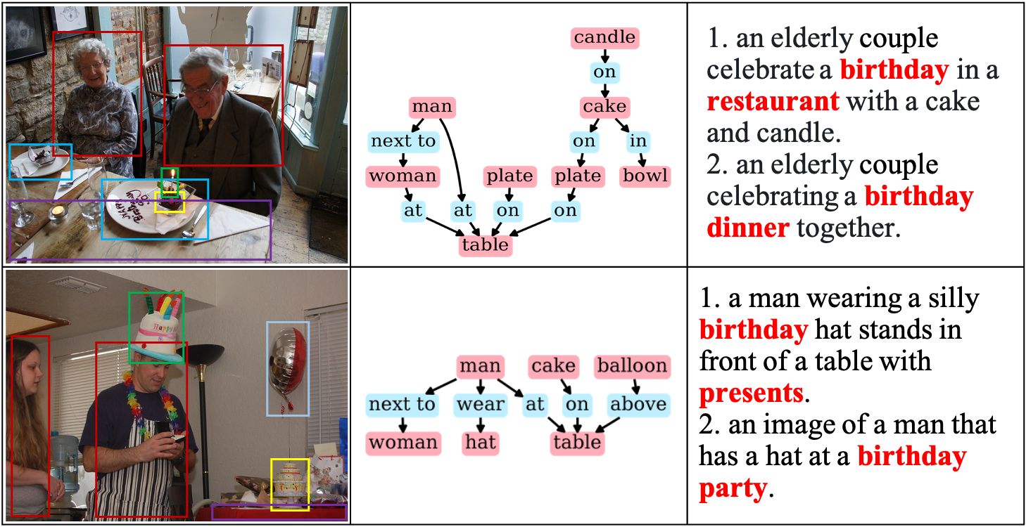
Figure 1: Examples of images, corresponding scene graphs and human-annotated captions. Text in red stands for theme concepts.

Existing researches on image captioning usually employ an encoder-decoder architecture Vinyals et al. (2015); Anderson et al. (2018) and focus on the problems of image representation learning and cross-modality semantic aligning Karpathy and Fei-Fei (2015); Ren et al. (2017).

For visual representation learning, the first generation of encoders splits an image into equal-sized regions and extracts CNN-based visual features Vinyals et al. (2015). In order to model objects in the image explicitly, Faster-RCNN Ren et al. (2015) is proposed to identify bounding boxes of concrete objects. Furthermore, scene graphs Yao et al. (2018); Yang et al. (2019) are introduced to incorporate relations among objects. In a scene graph, region features are extracted as objects and textual features are generated to describe relations. Although positive results have been reported of using scene graphs to represent images for downstream tasks, the semantic gap between visual signals and textual descriptions still exists.

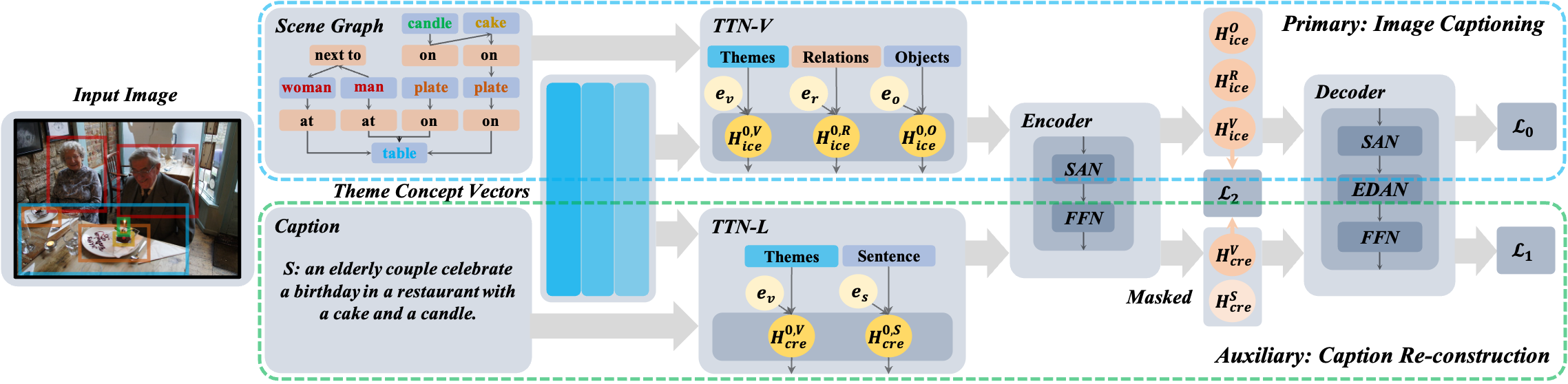
Figure 2: The framework of our proposed model Theme Concepts extended Image Captioner (TCIC). Theme concept vectors are used to represent the high-level cross-modality semantics. And they are updated by interacting with low-level facts in images and tokens in captions inside transformer structure TTN-V and TTN-L via two tasks of image captioning and caption re-construction respectively.

Figure 1 presents two examples with images, the corresponding scene graphs and descriptions constructed by humans. On the vision side, scene graph parser identifies some low-level facts of objects (“table”, “cake”, “man”, “candle”, “hat”, etc.) and relations (“on”, “next to”, etc.). On the language side, human annotators use some abstract concepts (“birthday”, “dinner”, “party”, etc.) of high-level semantics to describe images. This uncovers the semantic gap between the scene graph based visual representation and human language. Therefore, we argue that high-level semantic concepts (also called theme concepts in this paper) can be an extension to scene graphs to represent images. For semantic modeling of images, existing research constructs a list of concept words from descriptions in advance You et al. (2016); Gan et al. (2017a); Li et al. (2019); Fan et al. (2019), and train an independent module to attach these concept words to images as the guidance for image captioning. Instead of using a pre-defined list of words, we explore to represent theme concepts as shared latent vectors and learn their representations from both images and captions.

Inspired by the success of Transformer Herdade et al. (2019); Li et al. (2019) for image captioning, we propose Transformer with Theme Node (TTN) to incorporate theme concepts in the encoder of our architecture. On the vision side, theme concepts can be inferred based on reasoning over low-level facts extracted by scene graphs. For example, “birthday” can be inferred by different combinations of low-level facts, i.e., candle on cake, cake and balloon on table and man wear hat. Therefore, TTN is configured to integrate three kinds of information (noted as TTN-V), namely, objects, relations and theme concepts for visual representation modeling. Inside TTN-V, theme concept vectors work as theme nodes and their representations are updated by reasoning over nodes of objects and relations. On the language side, we introduce an auxiliary task named caption re-construction to enable the learning of theme concepts from text corpus. TTN is configured to integrate both text information and theme concepts (noted as TTN-L). It takes both them concept vectors and captions as input for caption re-construction. Both tasks share the same Transformer-based decoder for caption generation. Besides, we align representations of theme concepts learned from TTN-V and TTN-L for image-caption pairs to further enforce the cross-modality learning.

We conduct experiments on MS COCO Lin et al. (2014). Both offline and online testings show the effectiveness of our model compared to some state-of-the-art approaches in terms of automatic evaluation metrics. We further interpret the semantics of theme concepts via their related objects in the image and words in the caption. Results show that theme concepts are able to bridge the semantics of language and vision to some extent.

2 Related Work

Motivated by the encoder-decoder architecture, models produce texts from from image have many variants and improvement You et al. (2016); Anderson et al. (2018); Yang et al. (2019); Fan et al. (2018); Wang et al. (2020); Fan et al. (2019). In image captioning, Fang et al. (2015), You et al. (2016), Gan et al. (2017b) and Liu et al. (2019) pre-define a list of words as semantic concepts for image captioning.  You et al. (2016) employ an attention mechanism over word-level concepts to enhance the generator.  Li et al. (2019) propose to simultaneously exploit word concepts and visual information in decoder.

Some researchers also explore Transformer-based model for image captioning Li et al. (2019); Liu et al. (2019); Huang et al. (2019); Herdade et al. (2019); Cornia et al. (2020).  Herdade et al. (2019) propose to better model the spatial relations between detected objects through geometric attention.  Huang et al. (2019) extend self-attention to determine the relevance between attention outputs and query objects for refinement.  Cornia et al. (2020) introduce persist memory to self-attention key-value pairs as prior knowledge to enhance the generation.

The most relevant works to our research are HIP Yao et al. (2019), MMT Cornia et al. (2020) and SGAE Yang et al. (2019). Both HIP Yao et al. (2019) and our work explore to model structure information of images. HIP utilizes Mask R-CNN to identify instances in region via image segmentation. Our model is built on top of scene graph and is able to identify high-level semantics of the whole image. Our assumption is that objects spread in different corners of the image can also express the high-level semantics together, therefore, our model utilizes the low-level facts in the scene graph to explore high-level semantics. All of SGAE, MMT and our work utilize memory vectors, but the memory vectors of SGAE and MMT are fixed and non-interactive, which means that their memory vectors only provide prior information and are unable to actively learn the cross-modality theme concepts. In our framework theme concept vectors are learned by interacting with low-level facts in images and tokens in captions based on Transformer.

3 Theme Concepts Extended Image Captioning

The overall framework of our model Theme Concepts extended Image Captioning (TCIC) is shown in Figure 2. We model theme concepts as shared memory vectors ($\mathcal{V}$) and learn their representations inside Transformer with Theme Node (TTN) from both images and captions via two tasks. The primary task is image captioning (upper). TTN is configured as TTN-V to learn the visual representation for image captioning. It takes scene graph features (objects $\mathcal{O}$ and relations $\mathcal{R}$) and theme concepts $\mathcal{V}$ as input.

$$\mathcal{G}_{\theta}\big{(}\mathcal{V},\mathcal{O},\mathcal{R}\big{)}\rightarrow\mathcal{S}$$ (1)

The auxiliary task is caption re-construction (bottom). TTN is configured as TTN-L to learn the text representation for caption re-construction. It takes both textual features $\mathcal{S}$ and theme concepts $\mathcal{V}$ as input.

$$\mathcal{G}_{\theta}\big{(}\mathcal{V},\mathcal{S}\big{)}\rightarrow\mathcal{S}$$ (2)

Note that both TTN-V and TTN-L share the same architecture and parameters. Besides, we use the same decoder for caption generation in both tasks. During the training, representations of theme nodes learned in TTN-V ($\mathcal{H}_{ice}^{\mathcal{V}}$) and TTN-L ($\mathcal{H}_{cre}^{\mathcal{V}}$) are further aligned.

3.1 Image Encoder with TTN-V

The image encoder utilizes TTN-V to incorporate both scene graph features and theme concept vectors for image representation learning.

Inputs of TTN-V.

We extract objects $\mathcal{O}$ and relations $\mathcal{R}$ as the scene graph $\mathcal{SG}$ of the image. Then, theme concept vectors are used to extend $\mathcal{SG}$. Moreover, we employ multiple theme concept vectors to model image theme concepts from different aspects. Therefore, our image captioning inputs $\mathcal{I}_{ic}$ have three groups:

$$\mathcal{I}_{\emph{ic}}=\big{[}\mathcal{V},\mathcal{O},\mathcal{R}\big{]}$$ (3)

The three groups of nodes play different roles for visual semantics modeling, we utilize group embeddings, namely, $\big{\{}e_{o},e_{r},e_{v}\big{\}}\in\mathbb{R}^{d}$, to distinguish them as Eq. (4).

$$\mathcal{H}^{\emph{0}}_{\emph{ice}} =\left\{\begin{array}[]{ll}·\textbf{Emb}(v_{i})+e_{v},&v_{i}\in\mathcal{V}\vspace{1ex}\\ \textbf{W}_{\textbf{o}}\big{[}f_{i},p_{i}\big{]}+e_{o},&o_{i}\in\mathcal{O}\vspace{1ex}\\ \textbf{Emb}(r_{i})+e_{r},&r_{i}\in\mathcal{R}\end{array}\right.$$ (4)

where $\textbf{W}_{\text{o}}\in\mathbb{R}^{d\times(d_{o}+5)}$ is a trainable matrix, $d_{o}$ is the region feature dimension and $d$ is the hidden dimension of our encoder. $f_{i}\in\mathbb{R}^{d_{o}}$ is the region context feature of object $o_{i}$. $p_{i}=\big{(}\frac{x_{1}}{w},\frac{y_{1}}{h},\frac{x_{2}}{w},\frac{y_{2}}{h},\frac{(y_{2}-y_{1})(x_{2}-x_{1})}{wh}\big{)}$, where $(x_{1},y_{1})$ and $(x_{2},y_{2})$ denote the coordinate of the bottom-left and top-right corner of object $o_{i}$, while $w$ and $h$ are the width and height of the input image. Emb is the embedding function of theme nodes and relations.

Model	Cross Entropy						RL
	B-1	B-4	M	R	C	S	B-1	B-4	M	R	C	S
	Single Model
NIC Vinyals et al. (2015)	-	29.6	25.2	52.6	94.0	-	-	31.9	25.5	54.3	106.3	-
Up-Down Anderson et al. (2018)	77.2	36.2	27.0	56.4	113.5	20.3	79.8	36.3	27.7	56.9	120.1	21.4
GCN-LSTM Yao et al. (2018)	77.3	36.8	27.9	57.0	116.3	20.9	80.5	38.2	28.5	58.3	127.6	22.0
TOiW Herdade et al. (2019)	76.6	35.5	27.8	56.6	115.4	21.2	80.5	38.6	28.7	58.4	128.3	22.6
SGAE Yang et al. (2019)	77.6	36.9	27.7	57.2	116.7	20.9	80.8	38.4	28.4	58.6	127.8	22.1
MMT Cornia et al. (2020)	-	-	-	-	-	-	80.8	39.1	29.2	58.6	131.2	22.6
TCIC [Ours]	78.1	38.3	28.5	58.0	121.0	21.6	80.9	39.7	29.2	58.6	132.9	22.4
	Ensemble Model
SGAEΣ Yang et al. (2019)	-	-	-	-	-	-	81.0	39.0	28.4	58.9	129.1	22.2
GCN-LSTMΣ Yao et al. (2018)	77.4	37.1	28.1	57.2	117.1	21.1	80.9	38.3	28.6	58.5	128.7	22.1
HIPΣ Yao et al. (2019)	-	38.0	28.6	57.8	120.3	21.4	-	39.1	28.9	59.2	130.6	22.3
MMTΣ Cornia et al. (2020)	-	-	-	-	-	-	81.6	39.8	29.5	59.2	133.2	23.1
TCICΣ [Ours]	78.8	39.1	29.1	58.5	123.9	22.2	81.8	40.8	29.5	59.2	135.3	22.5

Table 1: Overall performance of MS COCO offline testing. B-1, B-4, R, M, C and S are short for BLEU-1, BLEU-4, ROUGE, METEOR, CIDEr-D and SPICE, respectively. ${\Sigma}$ means ensemble model. Numbers in bold denote the best performance in each column.

Structure of Image Encoder.

Each encoder layer in the image encoder includes Self-Attention Network SAN and Feed-Forward Network FFN. It takes $\mathcal{H}^{\mathit{l-1}}_{\mathit{ice}}$ as inputs.

The key of SAN is multihead attention MHA as Eq. (5).

$$\small\begin{gathered}\textbf{MHA}(\text{Q},\text{K},\text{V})=\textbf{W}_{\textbf{o}}\big{[}\text{head}_{\text{1}},\cdots,\text{head}_{\text{m}}\big{]}\vspace{1ex}~{}\\ \text{head}_{\text{i}}=\textbf{Attn}\big{(}\textbf{W}_{\textbf{q}}\text{Q},\textbf{W}_{\textbf{k}}\text{K},\textbf{W}_{\textbf{v}}\text{V}\big{)}\end{gathered})$$ (5)

where m is the number of attention heads, and $\textbf{W}_{\textbf{o}}\in\mathbb{R}^{d\times d}$ is the trainable output matrix. Moreover, the attention function Attn maps a query and a set of key-value pairs to an output:

$$\small\begin{gathered}\textbf{Attn}(\text{Q},\text{K},\text{V})=\textbf{Softmax}\bigg{(}\frac{\text{Q}^{\text{T}}\text{K}}{\sqrt{d_{k}}}\bigg{)}\text{V}~{}\end{gathered}$$ (6)

where the queries $\text{Q}\in\mathbb{R}^{d_{k}\times n_{q}}$, keys $\text{K}\in\mathbb{R}^{d_{k}\times n_{k}}$ and values $\text{V}\in\mathbb{R}^{d_{k}\times n_{k}}$, $d_{k}$ is the attention hidden size, $n_{q}$ and $n_{k}$ are the number of query and key, respectively.

$\mathcal{SG}$ in the encoder input has the inherent structure, i.e., $(o_{i},r_{j},o_{k})$. Thus we adopt hard mask for the triplets in $\mathcal{SG}$ to inject the structure knowledge into MHA. In detail, a matrix $\text{M}\in\mathbb{R}^{|\mathcal{I}_{\mathit{ic}}|\times|\mathcal{I}_{\mathit{ic}}|}$ is initialized with all $0$. For any object $o_{i}\in\mathcal{O}$ and any relation $r_{j}\in\mathcal{R}$, if there does not exist any object $o_{k}\in\mathcal{O}$, such that $(o_{i},r_{j},o_{k})\in\mathcal{SG}$, then we set $\text{M}_{i,j}=-\infty$. Following Eq. (5), we add M to Attn and get MAttn.

$$\small\begin{gathered}\textbf{MAttn}(\text{Q},\text{K},\text{V},\text{M})=\textbf{Softmax}\bigg{(}\text{M}+\frac{\text{Q}^{\text{T}}\text{K}}{\sqrt{d_{k}}}\bigg{)}\text{V}~{}\end{gathered}$$ (7)

Through replacing Attn with MAttn, we build the masked multihead attention MMHA.The details of our image captioning encoder layer is shown in Eq. (8)

$$\widehat{\mathcal{H}}^{\mathit{l}}_{\mathit{ice}} =\textbf{LN}\big{(}\mathcal{H}^{\mathit{l-1}}_{\mathit{ice}}+\textbf{MMHA}\big{(}\mathcal{H}^{\mathit{l-1}}_{\mathit{ice}},\mathcal{H}^{\mathit{l-1}}_{\mathit{ice}},\mathcal{H}^{\mathit{l-1}}_{\mathit{ice}}\big{)}\big{)}$$ (8)

$$\mathcal{H}^{\mathit{l}}_{\mathit{ice}} =\textbf{LN}\big{(}\widehat{\mathcal{H}}^{\mathit{l}}_{\mathit{ice}}+\textbf{W}_{2}\ \textbf{ReLU}\big{(}\textbf{W}_{1}\widehat{\mathcal{H}}^{\mathit{l}}_{\mathit{ice}}\big{)}\big{)}$$

where LN is LayerNorm.

Through image captioning encoding, we get the outputs $\mathcal{H}^{\mathcal{E}}_{\mathit{ice}}$. It consists of $\mathcal{H}^{\mathcal{V}}_{\mathit{ice}}$, $\mathcal{H}^{\mathcal{O}}_{\mathit{ice}}$ and $\mathcal{H}^{\mathcal{R}}_{\mathit{ice}}$, corresponding to $\mathcal{V}$, $\mathcal{O}$ and $\mathcal{R}$.

3.2 Caption Encoder with TTN-L

The caption encoder utilizes TTN-L to incorporate both textural features and theme concept vectors for caption re-construction.

Inputs of TTN-L.

We concatenate the target sentence $\mathcal{S}$ and theme nodes $\mathcal{V}$ as inputs of the caption encoder $\mathcal{I}_{\emph{sr}}$ in Eq. (9).

$$\small\begin{gathered}\mathcal{I}_{\emph{sr}}=\big{[}\mathcal{V},\mathcal{S}]~{}\end{gathered}$$ (9)

We also use group embeddings, $\big{\{}e_{v},e_{s}\big{\}}$, to distinguish theme nodes and words of captions in the embedding function as Eq. (10).

$$\mathcal{H}^{\emph{0}}_{\mathit{cre}} =\left\{\begin{array}[]{ll}\mathbf{Emb}(v_{i})+e_{v},&v_{i}\in\mathcal{V}\vspace{1ex}\\ \mathbf{Emb}(s_{i})+\mathbf{Emb}_{\mathit{p}}(s_{i})+e_{s},&s_{i}\in\mathcal{S}\end{array}\right.$$ (10)

where Emb is the embedding function of theme nodes and words, and $\textbf{Emb}_{\mathit{p}}$ is the position embedding following Vaswani et al. (2017).

Structure of Caption Encoder.

The caption encoder is the same as the image encoder except that it uses MHA instead of MMHA, but they share the same parameters. Taking $\mathcal{H}^{\mathit{0}}_{\mathit{cre}}$ as the input of the caption encoder, we get the outputs $\mathcal{H}^{\mathcal{E}}_{\mathit{cre}}$. It consists of $\mathcal{H}^{\mathcal{V}}_{\mathit{cre}}$ and $\mathcal{H}^{\mathcal{S}}_{\mathit{cre}}$, corresponding to $\mathcal{V}$ and $\mathcal{S}$.

3.3 Decoder for Caption Generation

We use the same decoder for both image captioning and caption re-construction. The embedding of decoder is initialized with $\mathcal{H}^{\mathit{0}}_{\mathit{icd}}$, which contains word embedding and position embedding following Vaswani et al. (2017).

In the $l$-th decoder layer, the inputs $\mathcal{H}^{\mathit{l-1}}_{\mathit{d}}$ go through SAN, EDAN and FFN.

$$\bar{\mathcal{H}}^{\mathit{l}}_{\mathit{d}} =\textbf{LN}\big{(}\mathcal{H}^{\mathit{l-1}}_{\mathit{d}}+\textbf{MHA}\big{(}\mathcal{H}^{\mathit{l-1}}_{\mathit{d}},\mathcal{H}^{\mathit{l-1}}_{\mathit{d}},\mathcal{H}^{\mathit{l-1}}_{\mathit{d}}\big{)}\big{)}$$ (11)

$$\widehat{\mathcal{H}}^{\mathit{l}}_{\mathit{d}} =\textbf{LN}\big{(}\bar{\mathcal{H}}^{\mathit{l}}_{\mathit{d}}+\textbf{MHA}\big{(}\bar{\mathcal{H}}^{\mathit{l}}_{\mathit{d}},\mathcal{H}^{\mathcal{E}}_{\mathit{e}},\mathcal{H}^{\mathcal{E}}_{\mathit{e}}\big{)}\big{)}$$

$$\mathcal{H}^{\mathit{l}}_{\mathit{d}} =\textbf{LN}\big{(}\widehat{\mathcal{H}}^{\mathit{l}}_{\mathit{d}}+\textbf{W}_{2}\ \textbf{ReLU}\big{(}\textbf{W}_{1}\widehat{\mathcal{H}}^{\mathit{l}}_{\mathit{d}}\big{)}\big{)}~{}$$

It is worth noting that, there is a difference between image captioning and caption re-construction in EDAN. For image captioning, $\bar{\mathcal{H}}^{\mathit{l}}_{\mathit{d}}$ are able to attend to all key-value pairs $\mathcal{H}^{\mathcal{E}}_{\mathit{ice}}$, but in caption re-construction, only the outputs of theme concept vectors, $\mathcal{H}^{\mathcal{V}}_{\mathit{cre}}$, are visible. Through this method, the theme concept vectors are encouraged to better capture the concept knowledge in captions $\mathcal{S}$.

$$\mathcal{H}^{\mathcal{E}}_{\mathit{e}} =\left\{\begin{array}[]{ll}\mathcal{H}^{\mathcal{E}}_{\mathit{ice}},\quad\text{image captioning}\vspace{1ex}\\ \mathcal{H}^{\mathcal{V}}_{\mathit{cre}},\quad\text{caption re-construction}\end{array}\right.$$ (12)

We get the outputs $\mathcal{H}^{\mathcal{D}}_{\mathit{d}}$ after decoding. At last, $\mathcal{H}^{\mathcal{D}}_{\mathit{d}}$ is utilized to estimate the word distribution as Eq. (13).

$$\textbf{P}(\mathcal{S})=\text{Softmax}\big{(}\textbf{W}_{d}\mathcal{H}^{\mathcal{D}}_{\mathit{d}}+b_{d}\big{)}{}$$ (13)

3.4 Overall Training

Our training has two phases, cross-entropy based training and RL based training. For cross-entropy based training, the objective is to minimize the negative log-likelihood of $\mathcal{S}$ given $\mathcal{I}_{\mathit{ic}}$, $\mathcal{L}_{0}$, and the negative log-likelihood of $\mathcal{S}$ given $\mathcal{I}_{\mathit{sr}}$, $\mathcal{L}_{1}$. To align the learning of theme concept vectors cross language and images, we add $\mathcal{L}_{2}$ to minimize the distance between $\mathcal{H}^{\mathcal{V}}_{\mathit{ice}}$ and $\mathcal{H}^{\mathcal{V}}_{\mathit{cre}}$.

$$\small\begin{gathered}\mathcal{L}_{0}=-\log\textbf{P}\big{(}\mathcal{S}|\mathcal{I}_{\mathit{ic}},\mathcal{G}_{\theta}\big{)},\ \mathcal{L}_{1}=\log\textbf{P}\big{(}\mathcal{S}|\mathcal{I}_{\mathit{sr}},\mathcal{G}_{\theta}\big{)}\\ \mathcal{L}_{2}=\big{\|}\mathcal{H}^{\mathcal{V}}_{\mathit{ice}}/\|\mathcal{H}^{\mathcal{V}}_{\mathit{ice}}\|_{2}^{2}-\mathcal{H}^{\mathcal{V}}_{\mathit{cre}}/\|\mathcal{H}^{\mathcal{V}}_{\mathit{cre}}\|_{2}^{2}\big{\|}_{2}^{2}\\ \mathcal{L}=\mathcal{L}_{0}+\lambda_{1}\mathcal{L}_{1}+\lambda_{2}\mathcal{L}_{2}\end{gathered}$$ (14)

where $\lambda_{1}$ and $\lambda_{2}$ are the factors to balance image captioning, caption re-construction and theme node alignments.

The next phase is to use reinforcement learning to finetune $\mathcal{G}_{\theta}$. Following Rennie et al. (2016), we use the CIDEr score as the reward function $r$ because it well correlates with the human judgment in image captioning Vedantam et al. (2015). Our training target is to maximize the expected reward of the generated sentence $\widehat{\mathcal{S}}$ as Eq. (15).

$$\max_{\theta}L_{\theta}=\max_{\theta}\mathbb{E}_{\widehat{S}\sim\mathcal{G}_{\theta}}\big{[}r(\widehat{\mathcal{S}})\big{]}$$ (15)

Then following the reinforce algorithm, we generate $K$ sentences, $\widehat{\mathcal{S}}_{\mathit{1}},\cdots,\widehat{\mathcal{S}}_{\mathit{K}}$, with the random sampling decoding strategy and use the mean of rewards as the baseline. The final gradient for one sample is thus in Eq. (16).

$$\small\begin{gathered}\bigtriangledown_{\theta}L_{\theta}=-\frac{1}{K}\sum_{k}\big{(}r(\widehat{S}_{k})-b_{k}\big{)}\bigtriangledown_{\theta}\log p(\widehat{\mathcal{S}}_{k}|\mathcal{I}_{\mathit{ic}},\mathcal{G}_{\theta})\\ b_{k}=\frac{1}{K-1}\sum_{j\neq k}r\big{(}\widehat{\mathcal{S}}_{j}\big{)}\end{gathered}$$ (16)

During prediction, we decode with beam search, and keep the sequence with highest predicted probability among those in the last beam.

4 Experiment and Results

Model		B-1	B-4	M	R	C
SGAEΣ	c5	81.0	38.5	28.2	58.6	123.8
	c40	95.3	69.7	37.2	73.6	126.5
HIPΣ	c5	81.6	39.3	28.8	59.0	127.9
	c40	95.9	71.0	38.1	74.1	130.2
TCICΣ	c5	81.8	40.0	29.2	59.0	129.5
	c40	96.0	72.9	38.6	74.5	131.4

Table 2: Overall performance of MS COCO online testing.

4.1 Experiment Setup

Offline and Online Evaluation.

We evaluate our proposed model on MS COCO Lin et al. (2014). Each image contains 5 human annotated captions. We split the dataset following Karpathy and Fei-Fei (2015) with 113,287 images in the training set and 5,000 images in validation and test sets respectively. Besides, we test our model on MS COCO online testing datasets (40,775 images). The online testing has two settings, namely c5 and c40, with different numbers of reference sentences for each image ( 5 in c5 and 40 in c40).

Single and Ensemble Models.

Following the common practice of model ensemble in Yao et al. (2018); Yang et al. (2019); Li et al. (2019), we build the ensemble version of TCIC through averaging the output probability distributions of multiple independently trained instances of models. We use ensembles of two instances, and they are trained with different random seeds.

Evaluation Metrics.

We use BLEU Papineni et al. (2002), METEOR Banerjee and Lavie (2005), ROUGE-L Lin and Hovy (2003), CIDEr Vedantam et al. (2015), and SPICE Anderson et al. (2016) as evaluation metrics, which are provided in COCO Caption Evaluation.

Models in Comparison.

We compare our model with some state-of-the-art approaches.

1. NIC Vinyals et al. (2015) is the baseline CNN-RNN model trained with cross-entropy loss.

2. Up-down Anderson et al. (2018) uses a visual attention mechanism with two-layer LSTM, namely, top-down attention LSTM and language LSTM.

3. GCN-LSTM Yao et al. (2018) presents Graph Convolutional Networks (GCN) to integrate both semantic and spatial object relations for better image encoding.

4. SGAE Yang et al. (2019) employs a pretrained sentence scene graph auto-encoder to model language prior, which better guide the caption generation from image scene graph.

5. TOiW Herdade et al. (2019) incorporates the object spatial relations to self-attention in Transformer.

6. HIP Yao et al. (2019) models a hierarchy from instance level (segmentation), region level (detection) to the whole image.

7. MMT Cornia et al. (2020) learns a prior knowledge in each encoder layer as key-value pairs, and uses a mesh-like connectivity at decoding stage to exploit features in different encoder layers.

8. TCIC is our proposed model.

4.2 Implementation Details

We utilize Faster-RCNN Ren et al. (2015) as the object detector and build the relation classifier following Zellers et al. (2018). On top of these two components, we build a scene graph for each image as the input of TTN-V. We prune the vocabulary by dropping words appearing less than five times. Our encoder has 3 layers and the decoder has 1 layer, the hidden dimension is 1024, the head of attention is 8 and the inner dimension of feed-forward network is 2,048. The number of parameters in our model is 23.2M. The dropout rate here is 0.3. We first train our proposed model with cross-entropy with 0.2 label smoothing, $(\lambda_{1},\lambda_{2})=(0.5,10.0)$ for 10k update steps, 1k warm-up steps, and then train it with reinforcement learning for 40 epochs, 40k update steps, $K$ in Eq. (16) is 5. We use a linear-decay learning rate scheduler with 4k warm-up steps, the learning rates for cross-entropy and reinforcement learning are 1e-3 and 8e-5, respectively. The optimizer of our model is Adam Kingma and Ba (2014) with (0.9, 0.999). The maximal region numbers per batch are 32,768 and 4,096. During decoding, the size of beam search is 3 and the length penalty is 0.1.

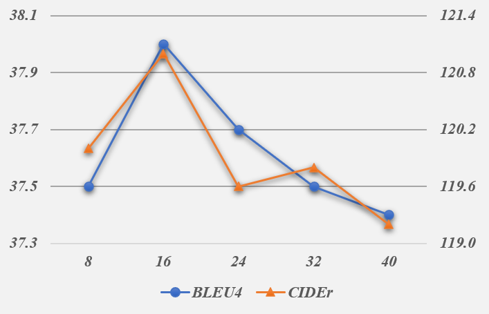
Figure 3: The performance of TCIC with different numbers of theme nodes (from 8 to 40, x-axis) in terms of CIDEr (right y-axis) and BLEU-4 (left y-axis).

4.3 Overall Performance

	B-1	B-4	M	R	C	S
T+$\mathcal{O}$	75.5	34.6	27.8	56.0	113.2	21.0
+$\mathcal{R}$	76.3	35.6	27.9	56.4	115.2	21.0
+$\mathcal{V}$	76.9	36.2	28.1	56.7	117.6	21.1
+GE	77.1	36.9	28.2	56.7	118.8	21.3
+CR	77.4	37.4	28.4	57.3	119.1	21.5
+TA	78.1	38.3	28.4	58.0	121.0	21.6

Table 3: Ablation study for TCIC. Components are added on top of the previous setting one by one from the first row to the bottom one.

We present the performance of offline testing in Table 1 with two configurations of results (Cross Entropy and RL). One is trained with cross-entropy loss and the other is further trained via reinforce algorithm using CIDEr score as the reward. For single models, TCIC achieves the highest scores among all compared methods in terms of most metrics (except BLEU-1 SPICE in RL version). For ensemble models, TCIC^Σ outperforms other models in all metrics (except SPICE in RL version). We also evaluate our ensemble model on the online MS COCO test server and results are shown in Table 2. TCIC^Σ also generates better results compared to other three models. This validates the robustness of our model.

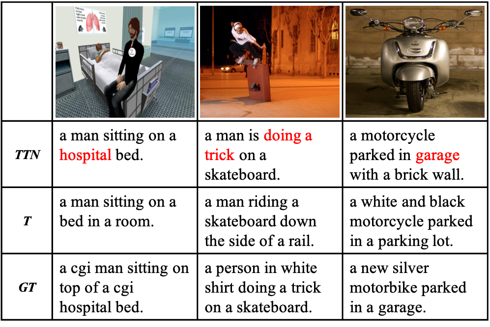
Figure 4: Sample captions from TCIC and Transformer.

4.4 Ablation Study

We perform ablation studies of our model. $\mathcal{O},\mathcal{R},\mathcal{V}$ stand for nodes of object, relation and theme concept vectors, respectively. T, GE, CR and TA are used to denote transformer, group embedding, caption re-construction and theme nodes alignment, respectively.

We add components into the basic setting one by one to track the effectiveness of the added component. We list results in Table 3. We can see that the performance increases as components are added one by one. This demonstrates the effectiveness of different components.

5 Further Analysis

We qualify the influence of number of theme nodes in model performance in § 5.1, interpret the semantics of theme concepts in § 5.2, and present case studies in § 5.3.

5.1 Influence of Theme Node Number

We investigate the influence of the number of theme nodes on the model performance in terms of CIDEr and BLEU-4. The results are shown in Figure 3. With the number of theme nodes increasing, both scores rise in the beginning, peak at 16 and go down after. This phenomenon indicates when the number of theme nodes is small, their modeling capacity is not strong enough to model theme concepts in the image for caption generation. When the number of theme nodes gets larger, different theme nodes may conflict with each other, which hurts the performance.

5.2 Interpretation of Theme Nodes

Theme concepts are introduce to represent cross modality high-level semantics. Through linking theme nodes with objects in TTN-V and words in TTN-L based on attention scores, we try to visulize semantics of these theme nodes.

In TTN-V, for each object node $o_{i}$, we obtain its attention scores to theme nodes through SAN. If the attention score to $v_{j}$ ranks in the top-2, we link $v_{j}$ with $o_{i}$ and increase their closeness scores by 1. We pick about 8 objects out of top-20 for each theme node in terms of closeness score. Same procedures are done in TTN-L to link theme nodes and words through SAN. We list 3 theme nodes and their relevant objects and words in Table 4. We conclude that:

1. Different theme nodes are related to different categories of objects and words. node#1 is clothing, while node#2 is related to transportation. This indicates different theme nodes contain different high-level semantics.

2. There exists correlation between TTN-V and TTN-L. Theme node#3 in encoder and decoder are both related to food. This reveals that TTN is able to align semantics of vision and language to some extent.

	TTN-V	TTN-L
1	jacket, tie, jean,	shorts, shirt, attire,
	sneaker, belt, vest,	mitt, hats, clothes,
	short, uniform, hat	uniforms, clothing, suits
2	wheel, pavement, car,	vehicles, helmets,
	van, sidewalk, truck,	carriages, passengers,
	street, road, bus	transit, tracks, intersection
3	vegetable, tomato, fruit,	fries, slices, chips,
	onion, orange, broccoli,	eat, food, vegetables,
	banana, apple, meat	plates, pizzas, sandwiches

Table 4: The most related elements in TTN-V encoder and TTN-L encoder for theme node#1, #2 and #3.

5.3 Case Study

We show sample captions generated by T (transformer) and TCIC in Figure 4. T only describes the low-level facts of images, but TCIC infers high-level concepts (words in red) on top of these facts such as, “hospital”, “doing a trick” and “garage”.

6 Conclusion and Future Work

In this paper, we explore to use theme concepts to represent high-level semantics cross language and vision. Theme concepts are modeled as memory vectors and updated inside a novel transform structure TTN. We use two tasks to enable the learning of the theme concepts from both images and captions. On the vision side, TTN takes both scene graph based features and theme concept vectors for image captioning. On the language side, TTN takes textual features and theme concept vectors for caption re-construction. Experiment results show the effectiveness of our model and further analysis reveals that TTN is able to link high-level semantics between images and captions. In future, we would like to explore the interpretation of theme concept vectors in an explicit way. Besides, the application of theme concept vectors for other downstream tasks would also be an interesting direction to explore.

References

- Anderson et al. [2016] Peter Anderson, Basura Fernando, Mark Johnson, and Stephen Gould. Spice: Semantic propositional image caption evaluation. In ECCV, 2016.
- Anderson et al. [2018] Peter Anderson, Xiaodong He, Chris Buehler, Damien Teney, Mark Johnson, Stephen Gould, and Lei Zhang. Bottom-up and top-down attention for image captioning and visual question answering. In CVPR, 2018.
- Banerjee and Lavie [2005] Satanjeev Banerjee and Alon Lavie. METEOR: An automatic metric for MT evaluation with improved correlation with human judgments. In ACL, 2005.
- Cornia et al. [2020] Marcella Cornia, Matteo Stefanini, Lorenzo Baraldi, and Rita Cucchiara. Meshed-Memory Transformer for Image Captioning. In CVPR, 2020.
- Fan et al. [2018] Zhihao Fan, Zhongyu Wei, Piji Li, Yanyan Lan, and Xuanjing Huang. A question type driven framework to diversify visual question generation. In IJCAI, 2018.
- Fan et al. [2019] Zhihao Fan, Zhongyu Wei, Siyuan Wang, and Xuanjing Huang. Bridging by word: Image grounded vocabulary construction for visual captioning. In ACL, 2019.
- Fang et al. [2015] Hao Fang, Saurabh Gupta, Forrest Iandola, Rupesh K Srivastava, Li Deng, Piotr Dollár, Jianfeng Gao, Xiaodong He, Margaret Mitchell, John C Platt, et al. From captions to visual concepts and back. In CVPR, 2015.
- Gan et al. [2017a] Zhe Gan, Chuang Gan, Xiaodong He, Yunchen Pu, Kenneth Tran, Jianfeng Gao, Lawrence Carin, and Li Deng. Semantic compositional networks for visual captioning. In CVPR, 2017.
- Gan et al. [2017b] Zhe Gan, Chuang Gan, Xiaodong He, Yunchen Pu, Kenneth Tran, Jianfeng Gao, Lawrence Carin, and Li Deng. Semantic compositional networks for visual captioning. In CVPR, 2017.
- Herdade et al. [2019] Simao Herdade, Armin Kappeler, Kofi Boakye, and Joao Soares. Image captioning: Transforming objects into words. In H. Wallach, H. Larochelle, A. Beygelzimer, F. d'Alché-Buc, E. Fox, and R. Garnett, editors, NeurIPS. 2019.
- Huang et al. [2019] Lun Huang, Wenmin Wang, Jie Chen, and Xiao-Yong Wei. Attention on attention for image captioning. In ICCV, 2019.
- Karpathy and Fei-Fei [2015] Andrej Karpathy and Li Fei-Fei. Deep visual-semantic alignments for generating image descriptions. In CVPR, 2015.
- Kingma and Ba [2014] Diederik P Kingma and Jimmy Ba. Adam: A method for stochastic optimization. arXiv, 2014.
- Li et al. [2019] Guang Li, Linchao Zhu, Ping Liu, and Yi Yang. Entangled transformer for image captioning. In ICCV, 2019.
- Lin and Hovy [2003] Chin-Yew Lin and Eduard Hovy. Automatic evaluation of summaries using N-gram co-occurrence statistics. In NAACL, 2003.
- Lin et al. [2014] Tsung-Yi Lin, Michael Maire, Serge Belongie, James Hays, Pietro Perona, Deva Ramanan, Piotr Dollár, and C Lawrence Zitnick. Microsoft COCO: Common objects in context. In ECCV, 2014.
- Liu et al. [2019] Fenglin Liu, Yuanxin Liu, Xuancheng Ren, Xiaodong He, and Xu Sun. Aligning visual regions and textual concepts for semantic-grounded image representations. In NeurIPS, 2019.
- Papineni et al. [2002] Kishore Papineni, Salim Roukos, Todd Ward, and Wei-Jing Zhu. BLEU: a method for automatic evaluation of machine translation. In ACL, 2002.
- Ren et al. [2015] Shaoqing Ren, Kaiming He, Ross Girshick, and Jian Sun. Faster r-cnn: Towards real-time object detection with region proposal networks. In NeurIPS, 2015.
- Ren et al. [2017] Zhou Ren, Xiaoyu Wang, Ning Zhang, Xutao Lv, and Li-Jia Li. Deep reinforcement learning-based image captioning with embedding reward. In CVPR, 2017.
- Rennie et al. [2016] Steven J. Rennie, Etienne Marcheret, Youssef Mroueh, Jarret Ross, and Vaibhava Goel. Self-critical sequence training for image captioning. CoRR, 2016.
- Vaswani et al. [2017] Ashish Vaswani, Noam Shazeer, Niki Parmar, Jakob Uszkoreit, Llion Jones, Aidan N Gomez, Ł ukasz Kaiser, and Illia Polosukhin. Attention is all you need. In NeurIPS. 2017.
- Vedantam et al. [2015] Ramakrishna Vedantam, C Lawrence Zitnick, and Devi Parikh. Cider: Consensus-based image description evaluation. In CVPR, 2015.
- Vinyals et al. [2015] Oriol Vinyals, Alexander Toshev, Samy Bengio, and Dumitru Erhan. Show and tell: A neural image caption generator. In CVPR, 2015.
- Wang et al. [2020] Ruize Wang, Zhongyu Wei, Piji Li, Qi Zhang, and Xuanjing Huang. Storytelling from an image stream using scene graphs. In AAAI, 2020.
- Yang et al. [2019] Xu Yang, Kaihua Tang, Hanwang Zhang, and Jianfei Cai. Auto-encoding scene graphs for image captioning. In CVPR, 2019.
- Yao et al. [2018] Ting Yao, Yingwei Pan, Yehao Li, and Tao Mei. Exploring visual relationship for image captioning. In ECCV, 2018.
- Yao et al. [2019] Ting Yao, Yingwei Pan, Yehao Li, and Tao Mei. Hierarchy parsing for image captioning. In ICCV, 2019.
- You et al. [2016] Quanzeng You, Hailin Jin, Zhaowen Wang, Chen Fang, and Jiebo Luo. Image captioning with semantic attention. In CVPR, 2016.
- Zellers et al. [2018] Rowan Zellers, Mark Yatskar, Sam Thomson, and Yejin Choi. Neural motifs: Scene graph parsing with global context. In CVPR, 2018.