Spectral index of synchrotron emission:
insights from the diffuse and magnetised interstellar medium

Abstract

Context. The interpretation of Galactic synchrotron observations is complicated by the degeneracy between the strength of the magnetic field perpendicular to the line of sight (LOS), $B_{\perp}$, and the cosmic-ray electron (CRe) spectrum. Depending on the observing frequency, an energy-independent spectral energy slope $s$ for the CRe spectrum is usually assumed: $s=-2$ at frequencies below $\simeq$400 MHz and $s=-3$ at higher frequencies.

Aims. Motivated by the high angular and spectral resolution of current facilities such as the LOw Frequency ARray (LOFAR) and future telescopes such as the Square Kilometre Array (SKA), we aim to understand the consequences of taking into account the energy-dependent CRe spectral energy slope on the analysis of the spatial variations of the brightness temperature spectral index, $\beta$, and on the estimate of the average value of $B_{\perp}$ along the LOS.

Methods. We illustrate analytically and numerically the impact that different realisations of the CRe spectrum have on the interpretation of the spatial variation of $\beta$. We use two snapshots from 3D magnetohydrodynamic simulations as input for the magnetic field, with median magnetic field strength of $\simeq 4$ and $\simeq 20\leavevmode\nobreak\ \mu$G, to study the variation of $\beta$ over a wide range of frequencies ($\simeq 0.1-10$ GHz).

Results. We find that the common assumption of an energy-independent $s$ is valid only in special cases. We show that for typical magnetic field strengths of the diffuse ISM ($\simeq$2$-$20 $\mu$G), at frequencies of 0.1$-$10 GHz, the electrons that are mainly responsible for the synchrotron emission have energies in the range $\simeq$100 MeV$-$50 GeV. This is the energy range where the spectral slope, $s$, of CRe has its greatest variation. We also show that the polarisation fraction can be much smaller than the maximum value of $\simeq 70\%$ because the orientation of ${\bf B}_{\perp}$ varies across the telescope’s beam and along the LOS. Finally, we present a look-up plot that can be used to estimate the average value of $B_{\perp}$ along the LOS from a set of values of $\beta$ measured at different frequencies, for a given CRe spectrum.

Conclusions. In order to interpret the spatial variations of $\beta$ observed from centimetre to metre wavelengths across the Galaxy, the energy-dependent slope of the Galactic CRe spectrum in the energy range $\simeq$100 MeV$-$50 GeV must be taken into account.

1 Introduction

Studies of diffuse synchrotron emission and its polarisation play a key role in constraining properties of the magnetic fields and of the interstellar medium (ISM) in the Milky Way, especially the cosmic-ray electron (CRe) energy spectrum. They are also relevant for measurements of the cosmic microwave background radiation at high radio frequencies (e.g., Planck Collaboration IV, 2020, and references therein) and the cosmological 21 cm radiation from Cosmic Dawn and Epoch of Reionisation (EoR) at low radio frequencies (e.g., Bowman et al., 2018; Gehlot et al., 2019; Mertens et al., 2020; Trott et al., 2020). Galactic synchrotron emission is one of the main foreground contaminants in these cosmological experiments and its emission dominates the radio sky at frequencies below $10\leavevmode\nobreak\ {\rm GHz}$. It is therefore of great importance to understand in detail the spectral and spatial variations of Galactic synchrotron emission in order to successfully mitigate it in cosmological observations (for more details see a review by Chapman & Jelić 2019).

The spectrum of Galactic synchrotron emission is usually expressed in terms of the brightness temperature $T_{\nu}$ (defined in Sect. 2.1) characterised by a frequency-dependent spectral index $\beta(\nu)=d\log T_{\nu}/d\log\nu$. Spatial variations of $\beta$ in a given region of the sky reflect spatial variations of the CRe and magnetic field properties in the ISM along the line of sight (LOS) across that region. Full sky maps of Galactic synchrotron emission clearly show spatial variations of $\beta$ already at the angular resolution of $\simeq 5^{\circ}$ (Guzmán et al., 2011). Facilities providing at least three times this angular resolution such as the LOw Frequency ARray, LOFAR (van Haarlem et al., 2013), and in the near future the Square Kilometre Array, SKA (Dewdney et al., 2009), will be able to investigate even finer variations of $\beta$.

In terms of frequency, the observed synchrotron spectrum is flatter at low radio frequencies than at high radio frequencies (Roger et al., 1999; Guzmán et al., 2011). Typical values of $\beta$ estimated from observations at mid and high Galactic latitudes are $-2.59<\beta<-2.54\pm 0.01$ between 50 and 100 MHz (Mozdzen et al., 2019) and $-2.62\pm 0.02<\beta<-2.60$ between 90 and 190 MHz (Mozdzen et al., 2017), as measured recently by the Experiment to Detect the Global EoR Signature (EDGES). In contrast, in the frequency range 1.4$-$7.5 GHz, $\beta$ is $-2.81\pm 0.16$ (Platania et al., 1998). This difference in the spectral index at low and high radio frequencies is related to ageing of the CRe energy spectrum (hereafter simply “CRe spectrum”), $j_{e}(E)$.

As CRe propagate through the ISM, they lose energy by a number of energy-loss mechanisms that involve interactions with matter, magnetic fields, and radiation (Longair, 2011). These processes deplete the population of relativistic electrons and change their original energy (injection) spectrum. The knowledge of the Galactic CRe spectrum is a challenging subject that has seen significant advances only in recent years. A number of relevant results have been achieved at high energies (above $\simeq 10$ GeV) thanks to the detections of the Fermi Large Area Telescope (Fermi LAT; Ackermann et al., 2010), the balloon-borne Pamela experiment (Adriani et al., 2011), and the Alpha Magnetic Spectrometer (AMS-02) on board of the International Space Station (Aguilar et al., 2014). Only recently the two Voyager probes crossed the heliopause, overcoming the problem of solar modulation, and constraining $j_{e}(E)$ down to $E\simeq 3$ MeV. (Cummings et al., 2016; Stone et al., 2019). Yet, the origin and propagation of CRe partly remain unresolved due to the degeneracy of a number of parameters and uncertainty about the role of reacceleration, convection, and on the diffusion coefficient (see, e.g., Strong et al. 2007 and Grenier et al. 2015 for comprehensive reviews on this topic).

The uncertainties on the Galactic CRe spectrum limit the interpretation of Galactic synchrotron emission. Depending on the frequency of observation, it is usually assumed that the spectrum of the electrons contributing to the emission can be characterised by a single energy slope. In this paper we will show that this assumption results in an oversimplification and needs to be replaced by a more accurate modelling when interpreting observations from centimetre to metre wavelengths. This is especially the case for the recent LOFAR (van Haarlem et al., 2013) polarimetric observations (e.g. Jelić et al., 2015; Van Eck et al., 2017), where observed polarised structures were possibly associated with synchrotron radiation from neutral clouds. As suggested by Van Eck et al. (2017) and further supported by Bracco et al. (2020), the observed polarised synchrotron emission might be originating from low column density clouds of interstellar gas along the sight line composed of a mixture of warm and cold neutral hydrogen media, referred to as WNM and CNM, respectively.

In the light of these recent results, we partly focus on the effects of the energy-dependent CRe spectral energy slope at a few hundred MHz. However, we also highlight the impact of an energy-dependent energy slope at higher frequencies. This paper is organised as follows. In Sect. 2 we introduce the theory of synchrotron emission and illustrate the effects on the brightness temperature spectral index depending on the parameterisation of the CRe spectrum; in Sect. 3 we apply the above results first to a cloud modelled as a uniform slab, then to the diffuse, multiphase ISM with the help of 3D magnetohydrodynamic (MHD) simulations, that we then use in Sect. 4 to compute brightness temperature maps, the spectral index, and the polarisation fraction. In Sect. 5 we discuss the effect of the angular resolution of the observations and show a procedure for predicting the average strength of the magnetic field perpendicular to the LOS, $B_{\perp}$, once the CRe spectrum is set. In Sect. 6 we summarise the main findings.

2 Fundamentals of synchrotron emission

Above $\simeq 10$ GeV, the CRe spectrum, (i.e., the number of electrons per unit energy, time, area, and solid angle), is approximately a power law in energy, $j_{e}(E)\propto E^{s}$. The spectral energy slope (hereafter simply “spectral slope”), $s(E)=d\log j_{e}/d\log E$, has been measured in the solar neighbourhood by several probes: Fermi LAT established a spectral slope $s=-3.08\pm 0.05$ in the energy range 7 GeV–1 TeV (Ackermann et al., 2010), the Pamela experiment found $s=-3.18\pm 0.05$ above the energy region influenced by the solar wind ($>30$ GeV; Adriani et al. 2011), and AMS-02 determined $s=-3.28\pm 0.03$ in the energy range 19.0–31.8 GeV and $s=-3.15\pm 0.04$ in the range 83.4–290 GeV (Aguilar et al., 2014). At low energies the spectral slope measured by the two Voyager probes in the energy range $\simeq$3$-$40 MeV is $-1.30\pm 0.05$ (Cummings et al., 2016; Stone et al., 2019). Thus, at energies below $\simeq$10 GeV, the spectral slope is energy-dependent. As we will see, this has significant consequences on the spectrum of the synchrotron emission observed at frequencies of hundreds of MHz up to tens of GHz.

Generally, models and simulations developed for the interpretation of Galactic synchrotron emission assume that CRe contributing to the emission above and below 408 MHz have $s=-3$ and $s=-2$, respectively (see, e.g., Sun et al., 2008; Waelkens et al., 2009; Reissl et al., 2019; Wang et al., 2020). This simplification is usually made to avoid time-consuming calculations, and is based on observations supporting a flatter spectrum below 408 MHz (see, e.g., Reich & Reich, 1988a, b; Roger et al., 1999). In Sect. 2.2 we show that this assumption turns out to be inaccurate both at low and high frequencies, leading to a misinterpretation of the synchrotron observations, in particular of the spatial variations of the spectral index $\beta$. To support this claim we consider the two realisations of the local CRe spectrum by Orlando (2018) and Padovani et al. (2018) shown in Fig. 1. The former is based on multifrequency observations, from radio to $\gamma$ rays, and Voyager 1 measurements through propagation models, and is representative of intermediate Galactic latitudes ($10^{\circ}<|b|<20^{\circ}$) that include most of the local radio synchrotron emission within $\sim 1$ kpc around the Sun; the latter is given by an analytical four-parameter fitting formula that reproduces exactly the power-law behaviour measured at low and high energies (see also Ivlev et al., 2015). As shown by the inset in Fig. 1, the spectra by Orlando (2018) and that of Padovani et al. (2018) differ by less than $\sim 25$% over the range of energies of interest here, below $E\simeq 50$ GeV. As we will see in Sect. 3.1, synchrotron observations can also constrain these two parameterisations.

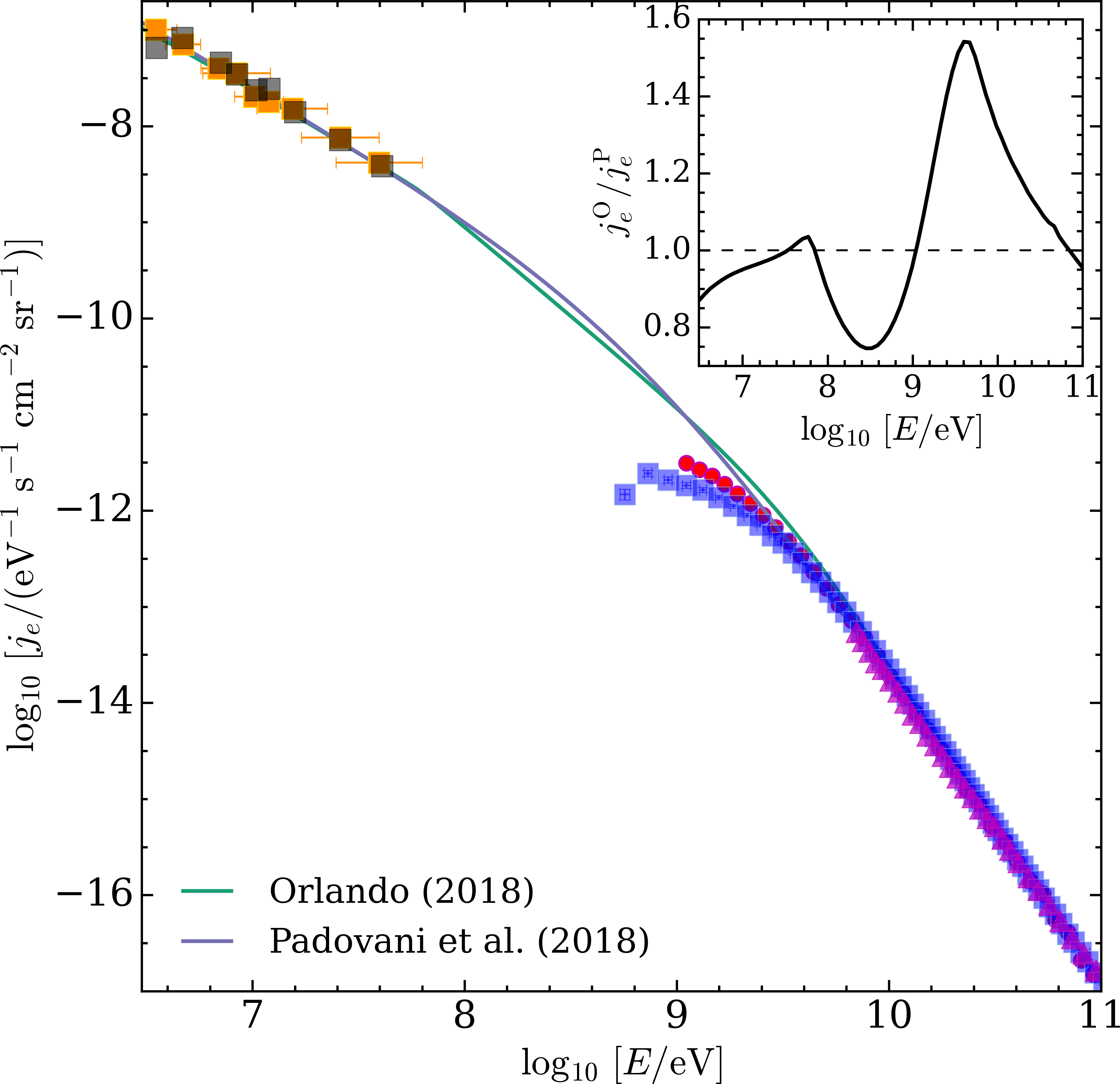
Figure 1: CRe spectrum according to Orlando (2018) (green line) and Padovani et al. (2018) (violet line). The inset shows the ratio of the spectra (O=Orlando, P=Padovani; solid black line). Data: Voyager 1 (orange squares; Cummings et al., 2016); Voyager 2 (grey squares; Stone et al., 2019); Fermi LAT (magenta triangles; Ackermann et al., 2010); Pamela (red circles; Adriani et al., 2011); AMS-02 (blue squares; Aguilar et al., 2014).

CRe at a given energy emit over a broad range of frequencies and, conversely, the synchrotron emission observed at a given frequency comes from a broad range of CRe energies. Before focusing on the frequency range of LOFAR observations (115–189 MHz; see Sect. 4), we consider frequency ranges characteristic of all-sky Galactic radio surveys both at low (45–408 MHz; Guzmán et al. 2011) and high frequencies (1–10 GHz; Platania et al. 1998). For $B_{\perp}\simeq 2$ to $20\leavevmode\nobreak\ \mu$G, as expected in the diffuse ISM (e.g., Heiles & Troland, 2005; Beck, 2015; Ferrière, 2020), CRe that account for nearly all of the observed synchrotron emission have energies ranging from $\simeq 100$ MeV to 50 GeV (see Sect. 2.2). In this energy range the spectral slope $s$ has a large variation with energy: between $-1.8$ and $-3.3$ and between $-1.5$ and $-3.2$, for the spectra modelled by Orlando (2018) and Padovani et al. (2018), respectively (see Fig. 2).

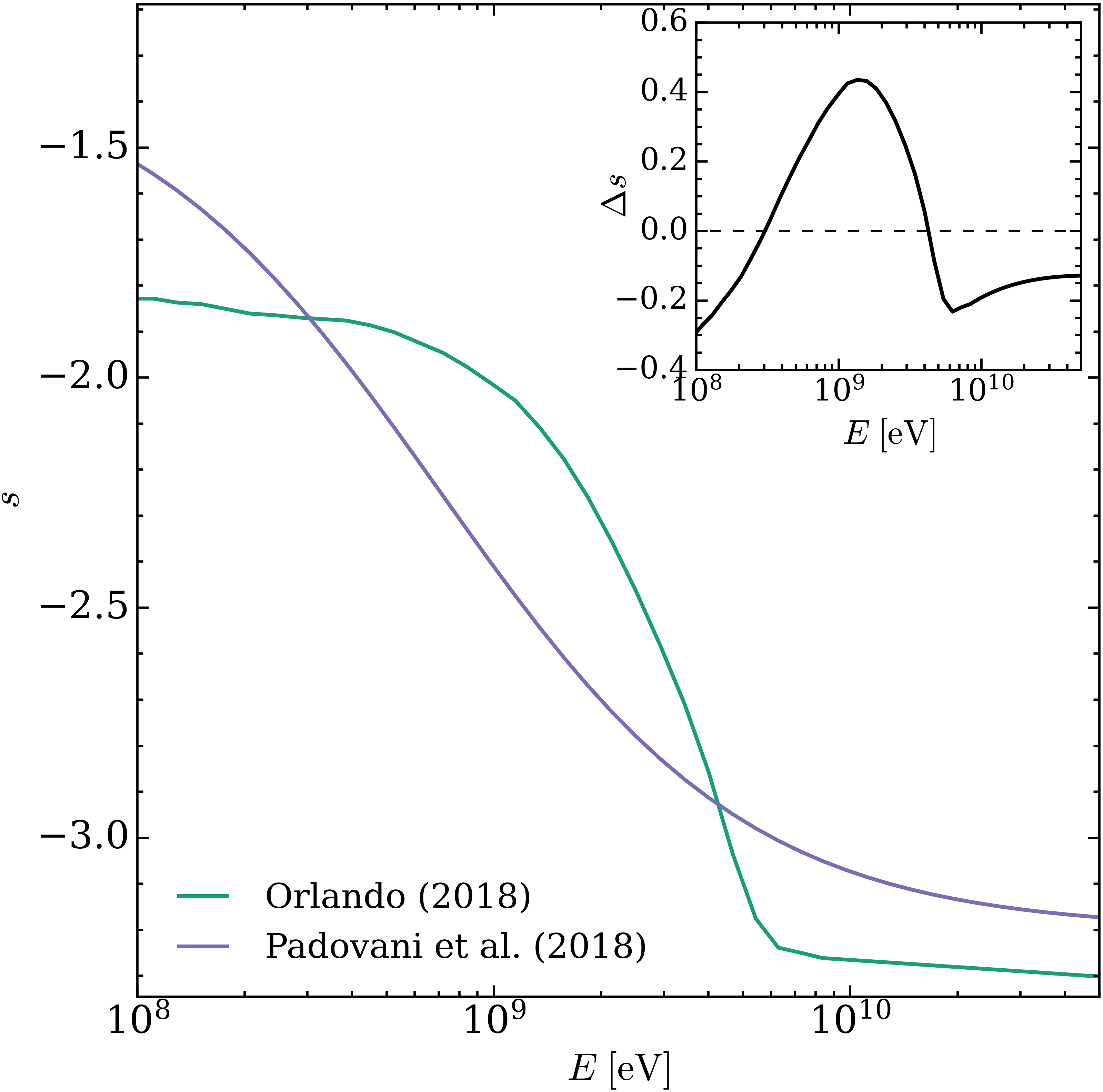
Figure 2: Spectral slope versus energy of the CRe spectra by Orlando (2018) (green line) and Padovani et al. (2018) (violet line) in the energy range relevant for our study (100 MeV$-$50 GeV). The inset shows the the difference $\Delta s$ between the spectral slope of the two spectra.

2.1 Basic equations

Here we summarise the basic equations for the calculation of the synchrotron brightness temperature, $T_{\nu}$ (see, e.g. Ginzburg & Syrovatskii, 1965, for details). At any given position ${\bf r}$ in a cloud, the specific emissivity can be split into two components linearly polarised along and across the component of the magnetic field perpendicular to the LOS, ${\bf B}_{\perp}$${\bf(r)}$,

$$\varepsilon_{\nu,\|}(\mathbf{r}) = \int_{m_{e}c^{2}}^{\infty}\frac{j_{e}(E)}{v_{e}(E)}P_{\nu,\|}^{\rm em}(E,\mathbf{r})\,{\rm d}E,$$ (1)

$$\varepsilon_{\nu,\perp}(\mathbf{r}) = \int_{m_{e}c^{2}}^{\infty}\frac{j_{e}(E)}{v_{e}(E)}P_{\nu,\perp}^{\rm em}(E,\mathbf{r})\,{\rm d}E\,,$$

where

$$P_{\nu,\|}^{\rm em}(E,\mathbf{r}) = \frac{\sqrt{3}e^{3}}{2m_{e}c^{2}}B_{\perp}(\mathbf{r})[F(x)-G(x)],$$ (2)

$$P_{\nu,\perp}^{\rm em}(E,\mathbf{r}) = \frac{\sqrt{3}e^{3}}{2m_{e}c^{2}}B_{\perp}(\mathbf{r})[F(x)+G(x)]$$

are the power per unit frequency emitted by an electron of energy $E$ at frequency $\nu$ for the two polarisations. Here, $B_{\perp}=|{\bf B}_{\perp}|$, $v_{e}$ is the electron velocity, $x=\nu/\nu_{c}$, and $\nu_{c}$ is the critical frequency given by

$$\nu_{c}[B_{\perp}(\mathbf{r}),E]=\frac{3eB_{\perp}(\mathbf{r})}{4\pi m_{e}c}\left(\frac{E}{m_{e}c^{2}}\right)^{2}\,.$$ (3)

The functions $F(x)$ and $G(x)$ are defined by

$$F(x)=x\int_{x}^{\infty}K_{5/3}(\xi){\rm d}\xi$$ (4)

and

$$G(x)=xK_{2/3}(x)\,,$$ (5)

where $K_{5/3}$ and $K_{2/3}$ are the modified Bessel functions of order 5/3 and 2/3, respectively. The corresponding Stokes $Q_{\nu}$ and $U_{\nu}$ specific emissivities are

$$\varepsilon_{\nu,Q}(\mathbf{r})=[\varepsilon_{\nu,\perp}(\mathbf{r})-\varepsilon_{\nu,\|}(\mathbf{r})]\cos[2\varphi(\mathbf{r})]$$ (6)

and

$$\varepsilon_{\nu,U}(\mathbf{r})=[\varepsilon_{\nu,\perp}(\mathbf{r})-\varepsilon_{\nu,\|}(\mathbf{r})]\sin[2\varphi(\mathbf{r})]\,,$$ (7)

where $\varphi({\bf r})$ is the local polarisation angle counted positively clockwise. The orientation of ${\bf B}_{\perp}$ rotated by $\pm 90^{\circ}$ gives the local polarisation angle (modulo $180^{\circ}$). The emissivities are integrated along the LOS to obtain the specific intensity (brightness) for each polarisation, $I_{\nu,\|}$ and $I_{\nu,\perp}$, and the Stokes parameters $Q_{\nu}$ and $U_{\nu}$. We also compute the polarisation fraction

$$p=\frac{P_{\nu}}{I_{\nu}}=\frac{\sqrt{Q_{\nu}^{2}+U_{\nu}^{2}}}{I_{\nu}}\,,$$ (8)

where $I_{\nu}=I_{\nu,\|}+I_{\nu,\perp}$. Finally, the flux density, $S_{\nu}$, obtained from the convolution of the specific intensity integrated along the LOS with the telescope beam, is converted into brightness temperature by the relation

$$T_{\nu}=10^{-23}\frac{S_{\nu}c^{2}}{2k_{\rm B}\Omega\nu^{2}}\leavevmode\nobreak\ {\rm K}\,,$$ (9)

where $\Omega=\pi\theta_{b}^{2}/(4\ln 2)$, $\theta_{b}$ is the full width of the beam at half its maximum intensity, and $k_{\rm B}$ is the Boltzmann constant. Here, $S_{\nu}$ is in Jy/beam and the other quantities are in cgs units. If the CRe spectrum is a single power law, $j_{e}(E)\propto E^{-s}$, then $S_{\nu}\propto\nu^{\alpha}$, with $\alpha=(s+1)/2$, and $T_{\nu}\propto\nu^{\beta}$, with $\beta=(s-3)/2$ (Ginzburg & Syrovatskii, 1965).

2.2 Contributions to synchrotron emission from 100 MHz to 10 GHz

In Sect. 2 we mentioned that the assumption of an energy-independent slope $s$ can introduce severe biases in the reliability of models and numerical simulations and ultimately affect the interpretation of synchrotron observations, such as the spatial variation of $\beta$. To prove this, we consider three observing frequencies (100 MHz, 1 GHz, and 10 GHz) representative of all-sky Galactic radio surveys (Platania et al., 1998; Guzmán et al., 2011) and two extreme values for $B_{\perp}$ (2 and 20 $\mu$G) consistent with the magnetic field strength expected in the diffuse medium (Heiles & Troland, 2005; Beck, 2015; Ferrière, 2020). To identify the range of energies contributing to the specific emissivity for a given value of $\nu$ and $B_{\perp}$, we examine the integrands $d\varepsilon_{\nu}/dE$ summed over the two polarisations (Eqs. (1)). As shown in the upper panels of Fig. 3, $d\varepsilon_{\nu}/dE$ has a well-defined maximum. For each frequency, we compute the energy range, around the energy of the maximum, where the specific emissivity is equal to 95% of its total. This fiducial 95% level is meant to show that most of the synchrotron emission at a given frequency originates from a definite, although broad, energy range of CRe. The resulting energy ranges (and the corresponding ranges of spectral slope $s$ derived for the CRe spectrum by Orlando 2018) are listed in Table 1. Looking at the ranges of $s$ at each frequency, it is clear that only in the extreme case of high frequencies ($\nu\gtrsim 10$ GHz) and very small $B_{\perp}$ ($\simeq 2\leavevmode\nobreak\ \mu$G), the hypothesis of an energy-independent spectral slope is accurate (in this case $s\simeq-3.3$). We note that the energy and the spectral slope intervals are the same for a given $\nu/B_{\perp}$ ratio. This is because the total power per unit frequency, $P^{\rm em}_{\nu}$, emitted at a frequency $\nu$ by an electron of energy $E$ in a field $B_{\perp}$, peaks at an energy proportional to $\sqrt{\nu/B_{\perp}}$ (see, e.g., Longair, 2011). Figure 3 shows that, for the typical frequency range of synchrotron observation in the diffuse ISM and for the expected values of $B_{\perp}$, CRe with energies between 100 MeV and 50 GeV are responsible for almost all the non-thermal emission. Since in this energy range the spectral slope has the largest variation, the assumption of an energy-independent $s$ is not correct.

For the sake of simplicity, we have only considered the case of the CRe spectrum by Orlando (2018). Using instead that of Padovani et al. (2018), the energy intervals we obtain are similar, as the two spectra differ on average by 25% (see Sect. 2 and Fig. 1). However, what changes are the spectral slope intervals (see Fig. 2). This means that the use of a particular CRe spectrum has a major influence on the interpretation of the observations. In the next section we show how observational estimates of the brightness temperature spectral index help to constrain the accuracy of a CRe spectrum.

Table 1: Ranges of energy $E$ and spectral slope $s$ for two values of $B_{\perp}$ and for a set of frequencies^a.

$\nu$ [GHz]	$B_{\perp}=2\leavevmode\nobreak\ \mu$G		$B_{\perp}=20\leavevmode\nobreak\ \mu$G
	$E$ [GeV]	$s$	$E$ [GeV]	$s$
0.1	[0.7,5.8]	[$-3.20,-1.94$]	[0.2,2.7]	[$-2.52,-1.86$]
1	[2.1,14.6]	[$-3.27,-2.33$]	[0.7,5.8]	[$-3.20,-1.94$]
10	[6.3,43.6]	[$-3.30,-3.24$]	[2.1,14.6]	[$-3.27,-2.33$]

^a  The ranges of $E$ and $s$ have been derived for the CRe spectrum by Orlando (2018) by integrating $d\varepsilon_{\nu}/dE$ in an energy range around the peak value until 95% of the total specific emissivity is recovered.

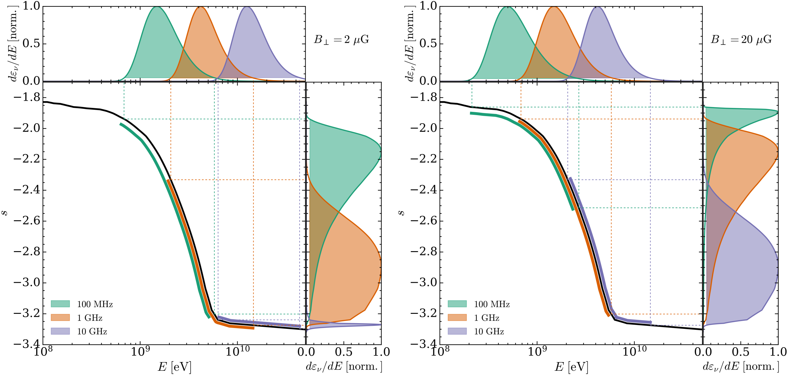
Figure 3: Left panel. Upper plot: integrand of the specific emissivity, $d\varepsilon_{\nu}/dE$, as a function of the energy $E$, normalised to its maximum value and summed over the two polarisations (Eqs. (1)), computed at 100 MHz, 1 GHz, and 10 GHz (green, orange, and violet line, respectively), for $B_{\perp}=2\leavevmode\nobreak\ \mu$G. The coloured area below each curve corresponds to the 95% of the total emissivity. Right plot: same as the upper plot, as a function of the CRe spectral slope $s$. Main plot: Spectral slope as a function of the energy for the CRe spectrum by Orlando (2018) (black solid line). Coloured lines show the range of energies (and the corresponding spectral slopes) contributing to 95% of the specific emissivity. Right panel: same as left panel, but for $B_{\perp}=20\leavevmode\nobreak\ \mu$G.

3 Modelling synchrotron emission

In this section we first consider a cloud modelled as a simple uniform slab to show how specific realisations of the CRe spectrum can be ruled out by comparison with observational estimates of $\beta$ (Sect. 3.1). We then describe the numerical simulations that we will use in the rest of the paper to study the spatial variations of $\beta$ and of the polarisation fraction (Sect. 3.2).

3.1 Uniform slab

To show the importance of an accurate modelling of the CRe spectrum, we compute the brightness temperature, $T_{\nu}$, for a slab with a fixed, spatially uniform, component of the magnetic field $B_{\perp}$, varying from 2 to 20 $\mu$G as specified in Sect. 2, exposed to a flux of CRe, $j_{e}(E)$, given by the Orlando (2018) and Padovani et al. (2018) spectra. For illustration, we select the frequency range $\nu=115$–189 MHz, with a frequency resolution of 183 kHz and assume an angular resolution of $\theta_{b}=4^{\prime}$. These parameters are representative of the LOFAR High Band Antenna observations carried out by Jelić et al. (2015). We assume a thickness of the slab of 1 pc, although the brightness temperature can be easily scaled for any different value. We then compute the spectral index, $\beta$, through a linear fit of $\log T_{\nu}$ versus $\log\nu$ for each $B_{\perp}$ value.

The brightness temperatures generated by the two realisations of the CRe spectrum are on average within $\simeq 25$% of each other (upper panel of Fig. 4), of the order of a few to several K. Assuming a synchrotron polarisation fraction of $p\approx 70$% (more details in Sect. 4.3) the polarised intensity would be of the same order as $T_{\nu}$. This is exactly the amount of diffuse polarised emission observed by LOFAR in the range 100–200 MHz (e.g., Jelić et al., 2014, 2015; Van Eck et al., 2017). These simple arguments support the scenario, suggested by Van Eck et al. (2017) and Bracco et al. (2020), where pc-scale neutral clouds in the diffuse ISM could significantly contribute to the Faraday-rotated synchrotron polarisation observed with LOFAR. However, if we compare the value of $\beta$ (lower panel of Fig. 4) with typical values derived from observations at intermediate and high Galactic latitudes (Mozdzen et al., 2017, shaded strip in the lower panel of Fig. 4), it is evident that in this example only the spectrum by Orlando (2018) is consistent with the observations, and only for values of $B_{\perp}$ of the order of 6–9 $\mu$G, while the one by Padovani et al. (2018) requires unrealistically high values of $B_{\perp}$. As this example illustrates, the constraint imposed by the highly accurate determination of the spectral index $\beta$ allowed by current instruments is a strong motivation to further and thoroughly model the synchrotron emission – total and polarised – of the diffuse ISM.

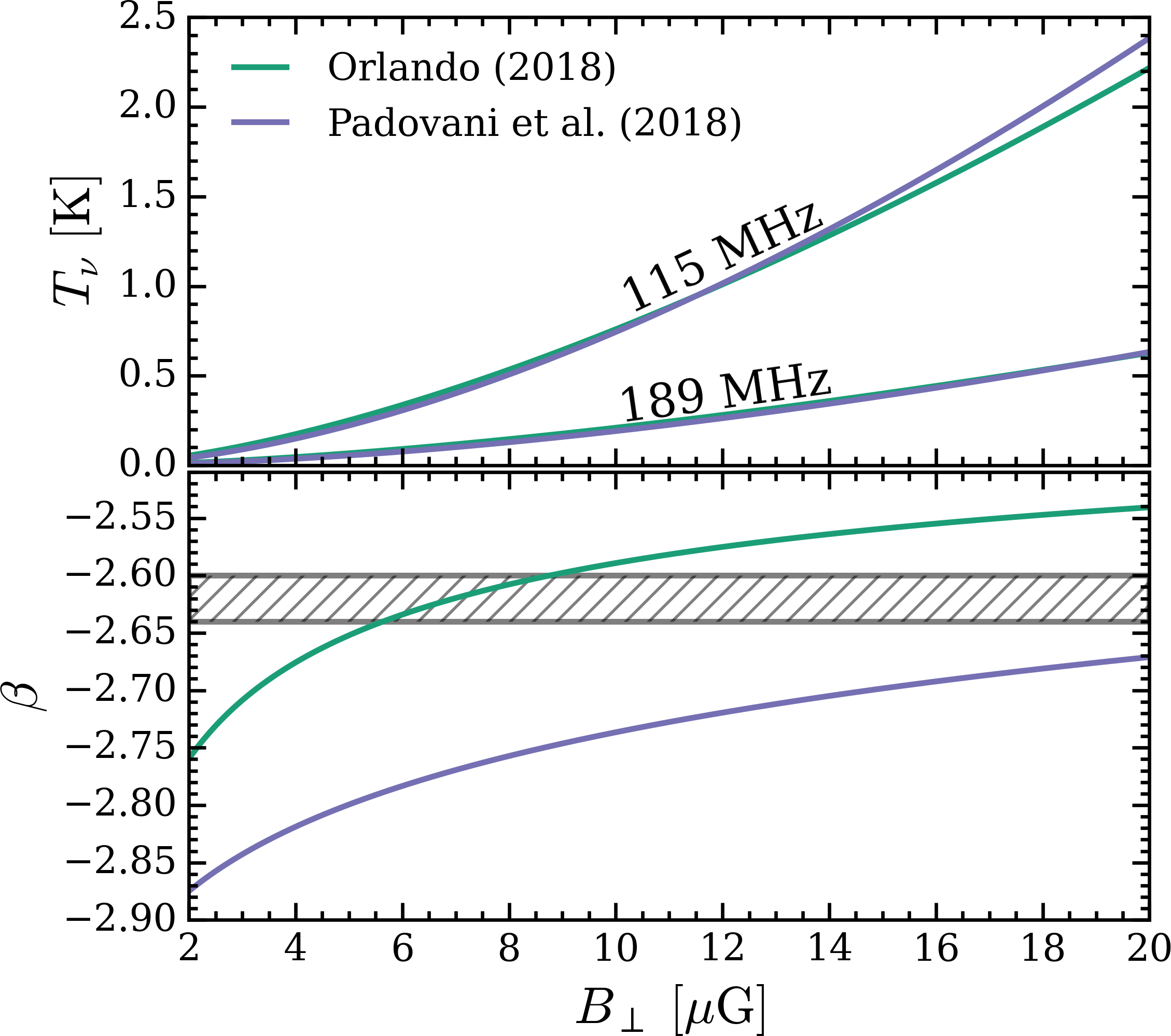
Figure 4: Upper panel: brightness temperature $T_{\nu}$ as a function of $B_{\perp}$  computed at $\nu=115$ and 189 MHz with the CRe spectra by Orlando (2018) (green line) and Padovani et al. (2018) (violet line) for a slab of thickness 1 pc, with an angular resolution $\theta_{b}=4^{\prime}$. Lower panel: brightness temperature spectral index $\beta$ as a function of $B_{\perp}$ (same colour coding as in the upper panel). The hatched region highlights typical values of $\beta$ at intermediate and high latitudes (Mozdzen et al., 2017).

3.2 Numerical simulations

We now compute synthetic observations of synchrotron emission adopting state-of-the-art numerical simulations of the diffuse, magnetised, multiphase, turbulent, and neutral atomic ISM. Our approach here is not to consider the simulations described below as true representations of any given LOS in the diffuse ISM, but rather as a laboratory to study realistic physical conditions of the multiphase medium where synchrotron emission may originate. In particular, we perform numerical simulations of the diffuse ISM using the RAMSES code (Teyssier, 2002; Fromang et al., 2006), a grid-based solver with adaptive mesh refinement (Berger & Oliger, 1984), and a fully-treated tree data structure (Khokhlov, 1998).

The gas density of the medium we consider is typically dominated by neutral hydrogen that can be traced via the 21 cm emission line (Heiles & Troland, 2003a, b; Murray et al., 2015, 2018). This line is usually decomposed into several Gaussian components (Kalberla & Haud, 2018; Marchal et al., 2019) associated to distinct gas phases in pressure balance: a dense cold neutral medium, CNM, with temperature and density $T\simeq 50$ K and $n_{\rm H}\simeq 50$ cm^-3, respectively, immersed in a diffuse warm neutral medium, WNM, with $T\simeq 8000$ K and $n_{\rm H}\simeq 0.3$ cm^-3, and a third intermediate unstable phase, with temperature comprised between those of the CNM and the WNM (e.g. Wolfire et al., 2003; Bracco et al., 2020). Field (1965) and Field et al. (1969) pointed out that the microphysical processes of heating and cooling naturally lead to two thermally stable (CNM and WNM) and a thermally unstable phases coexisting in a range of thermal pressure. Through the thermal processes of condensation and evaporation, and with the help of turbulent transport and turbulent mixing, the diffuse matter can flow from one stable state to the other.

The local diffuse matter in our Galaxy is simulated over a box of 50 pc with periodic boundary conditions, using a fixed grid of $128^{3}$ pixels, corresponding to an effective resolution of 0.39 pc. The initial state is characterised by a homogeneous density $n_{\rm H}=$1.5 cm^-3, a temperature $T=8000$ K, and a uniform magnetic field $\@vec{B}_{0}=B_{0}\hat{e}_{x}$. We consider two snapshots of the simulation, one with a standard average magnetic field strength, $B_{0}=4\leavevmode\nobreak\ \mu$G (hereafter “weak field” case), and one with a stronger $B_{0}=20\leavevmode\nobreak\ \mu$G (hereafter “strong field” case). The gas evolves under the joint influence of turbulence, magnetic field, radiation field, and thermal instability, and separates in three different phases: CNM, WNM, and unstable. A turbulent forcing is applied to mimic the injection of mechanical energy in the diffuse ISM. Following Schmidt et al. (2009) and Federrath et al. (2010), this forcing, modelled by an acceleration term in the momentum equation, is driven through a pseudo-spectral method. The turbulent acceleration parameter is set to $2.77\times 10^{-3}$ kpc Myr^-2. Using classical notation, the dimensionless compressible parameter for the turbulent forcing modes, $\zeta_{0}$, ranges from pure solenoidal modes ($\zeta_{0}=1$) to pure compressible modes ($\zeta_{0}=0$). We set $\zeta_{0}=0.5$.

The matter is assumed to be illuminated on all sides by an isotropic spectrum of UV photons set to the standard interstellar radiation field (Habing, 1968). To correctly describe the thermal state of the diffuse ISM, we have included the heating induced by the photoelectric effect on interstellar dust grains and secondary electrons produced during cosmic-ray propagation, and the cooling induced by emission of Lyman-$\alpha$ photons, the fine-structure lines of OI and CII, and the recombination of electrons onto grains. All these processes, described in Appendix B of Bellomi et al. (2020), are modelled with the analytical formulae given by Wolfire et al. (2003).

These simulations represent two different scenarios: in the “weak field” case, the magnetic field has a turbulent component of the same order of its mean component. By contrast, in the “strong field” case, the magnetic field is mostly directed along the $x$-axis, i.e. its projection is mainly contained in the $xy$ and $zx$ planes. The advantage of using simulations is that we can rotate each snapshot according to the three axes and calculate the quantities of interest integrated along three different LOS, thus increasing our statistics. Table 2 summarises the ranges of the strength of the magnetic field in the plane perpendicular to a given LOS and their median values (marked by a superscript tilde) for the two snapshots under consideration. Specifically, for the LOS $i$, we compute the minimum and maximum value of the magnetic field strength, $B_{jk}=(B_{j}^{2}+B_{k}^{2})^{1/2}$, in the plane of the sky (POS) $jk$. Subscripts $i$, $j$, and $k$ follow the cyclic permutation of Cartesian coordinates $(ijk)=\{xyz,yzx,zxy\}$.

Table 2: Minimum and maximum values of the strength of the magnetic field in the plane perpendicular to the LOS $i$, $B_{jk}=(B_{j}^{2}+B_{k}^{2})^{1/2}$, and its median value $\tilde{B}_{jk}$ for the two cases of weak and strong field^a.

	LOSi	$B_{jk}$ [$\mu$G]	$\tilde{B}_{jk}$ [$\mu$G]
weak field ($B_{0}=4\leavevmode\nobreak\ \mu$G)	$x$	[$1.1\times 10^{-3},12$]	$2.02^{+0.88}_{-0.75}$
	$y$	[$1.5\times 10^{-3},16$]	$4.26^{+0.73}_{-0.71}$
	$z$	[$9.8\times 10^{-3},13$]	$4.22^{+0.71}_{-0.74}$
strong field ($B_{0}=20\leavevmode\nobreak\ \mu$G)	$x$	[$3.6\times 10^{-4},6$]	$0.80^{+0.38}_{-0.30}$
	$y$	[$17,22$]	$19.19^{+0.33}_{-0.41}$
	$z$	[$17,22$]	$19.19^{+0.33}_{-0.40}$

^a  Errors on $\tilde{B}_{jk}$ are estimated using the first and third quartiles. Subscripts $i$, $j$, and $k$ follow the cyclic permutation of Cartesian coordinates $(ijk)=\{xyz,yzx,zxy\}$.

4 Results

In contrast to typical angular resolutions of earlier facilities, such as the $5^{\circ}$ of Guzmán et al. (2011), nowadays, LOFAR provides a significantly higher resolution, typically up to $4^{\prime}$ at frequencies of 115$-$189 MHz for observations of Galactic diffuse emission (Jelić et al., 2014, 2015; Van Eck et al., 2017). In the following, we show our results at the resolution of $6.7^{\prime}$. The latter value corresponds to the spatial resolution of the simulations (0.39 pc) if the simulation snapshots are placed at a distance of 200 pc. We focus on the frequency range 115$-$189 MHz, however the same conclusions apply to higher frequencies (see Sect. 5.2 and Appendix A).

4.1 Brightness temperature maps

Figure 5 shows the brightness temperature maps at a frequency $\nu=130$ MHz for the two snapshots described in Sect. 3.2, obtained with the CRe spectrum of Orlando (2018). These images are derived by integrating along the three different LOS ($x$, $y$, $z$) over the length of the snapshot (50 pc), resulting in temperature maps identified by the respective POS ($yz$, $zx$, $xy$). As anticipated by the upper panel of Fig. 4, the temperature is higher where $B_{\perp}$ is larger, reaching a maximum in the $xy$ and $zx$ POS of the strong field case (right column of Fig. 5; see also the values of $\tilde{B}_{jk}$ in Table 2), while the smallest temperature values are in the $yz$ POS of the strong field case. Temperature maps are more inhomogeneous in the $yz$ POS of both snapshots. That is because in these planes $B_{\perp}$ has a significant turbulent component. Therefore, we introduce the ratio between the standard deviation and the median value of $B_{\perp}$, $\mu=\sigma_{B_{\perp}}/\tilde{B}_{\perp}$, to quantify the relative turbulent component of $B_{\perp}$. This quantity, whose median values are reported in Table 3, is useful for the discussion on $\beta$ and on the polarisation fraction in the following two subsections.

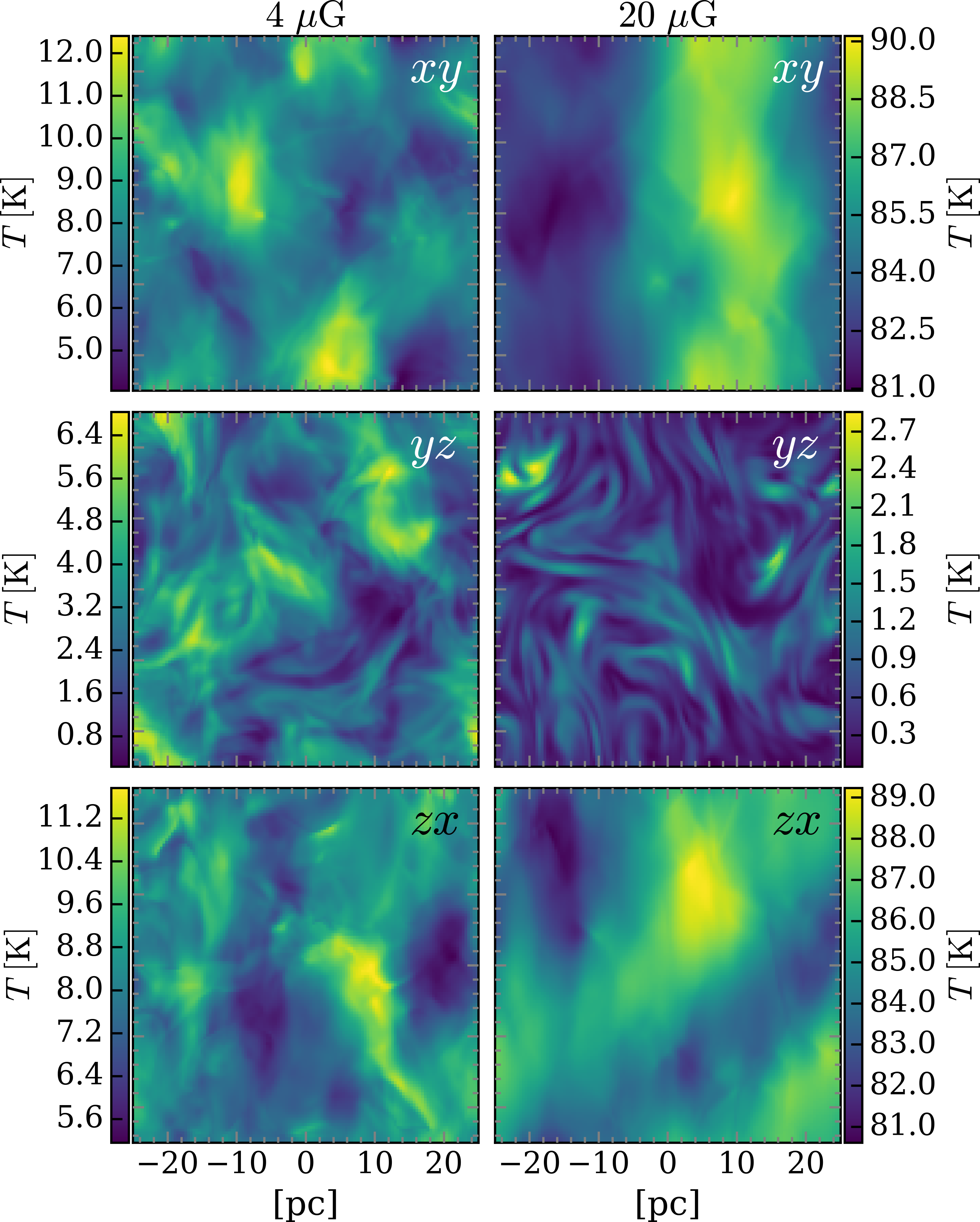
Figure 5: Brightness temperature maps (colour scale) computed with the Orlando (2018) spectrum, at $\nu=130$ MHz and with resolution $6.7^{\prime}$ for the three POS (three rows, labelled $xy$, $yz$, and $zx$) of the weak and strong field case (left and right column, respectively).

4.2 Brightness temperature spectral index

We compute the brightness temperature spectral index, $\beta$, for each LOS, by a linear fit of $\log T_{\nu}$ versus $\log\nu$ for the three POS of the two snapshots, in the frequency range 115–189 MHz with a frequency resolution of 183 kHz as in the LOFAR dataset by Jelić et al. (2015). In Fig. 6, we show the results in the form of bivariate and marginal distributions (see also Appendix B for the maps of $\beta$). From the inspection of Fig. 6, it is evident that in no case, at low frequencies, is $\beta$ equal to $-2.5$, as would follow from the assumption of constant $s=-2$. As shown in Sect. 2.2, the same consideration holds in the high frequency regime ($\nu\gtrsim 400$ MHz), where the assumption of constant $s=-3$, and hence $\beta=-3$, turns out to be incorrect. Figure 6 also shows that $\tilde{\beta}$ is less negative in the POS $xy$ and $zx$, where $\tilde{B}_{\perp}$ is larger (see also Tables 2 and 3). This is a consequence of what is shown in Fig. 3: for a given frequency, the larger the value of $B_{\perp}$ at a given position along the LOS, the smaller the median value of the energy range determining its synchrotron emissivity. Therefore, the corresponding values of $s$, and hence of $\beta$, increase. Finally, an important aspect to note is that the dispersion of $\beta$ values around its median depends weakly on $\mu$. Indeed, in both $yz$ POS, where $\mu$ reaches the largest values, the interquartile range (i.e. the difference between the third and the first quartile) is only 0.04 and 0.06 for the weak and the strong case, respectively. For the sake of completeness, in Appendix A we show the bivariate distributions of $\mu$ and $\beta$ for higher frequency ranges (467$-$672 MHz and 833$-$1200 MHz), which will be used later in Sect. 5.2. The conclusions are the same as for the 115$-$189 MHz range.

Table 3: Medians of the ratio between the standard deviation of $B_{\perp}$ and its median value, $\mu=\sigma_{B_{\perp}}/\tilde{B}_{\perp}$, of the brightness temperature spectral index, and of the polarisation fraction at a resolution of $6.7^{\prime}$ for the three POS and the two cases of weak and strong field^a.

	POS	$\tilde{\mu}$	$\tilde{\beta}$	$\tilde{p}$
weak field ($B_{0}=4\leavevmode\nobreak\ \mu$G)	$xy$	$0.23^{+0.06}_{-0.05}$	$-2.66\pm 0.01$	$0.57^{+0.05}_{-0.06}$
	$yz$	$0.51^{+0.14}_{-0.10}$	$-2.72\pm 0.02$	$0.34\pm 0.10$
	$zx$	$0.24^{+0.05}_{-0.05}$	$-2.66\pm 0.01$	$0.55\pm 0.06$
strong field ($B_{0}=20\leavevmode\nobreak\ \mu$G)	$xy$	$0.02\pm 0.01$	$-2.54$	$0.70$
	$yz$	$0.47^{+0.12}_{-0.09}$	$-2.84\pm 0.03$	$0.51^{+0.09}_{-0.13}$
	$zx$	$0.02\pm 0.01$	$-2.54$	$0.70$

^a  Errors have been estimated using the first and third quartiles. Errors smaller than 0.01 are not shown.

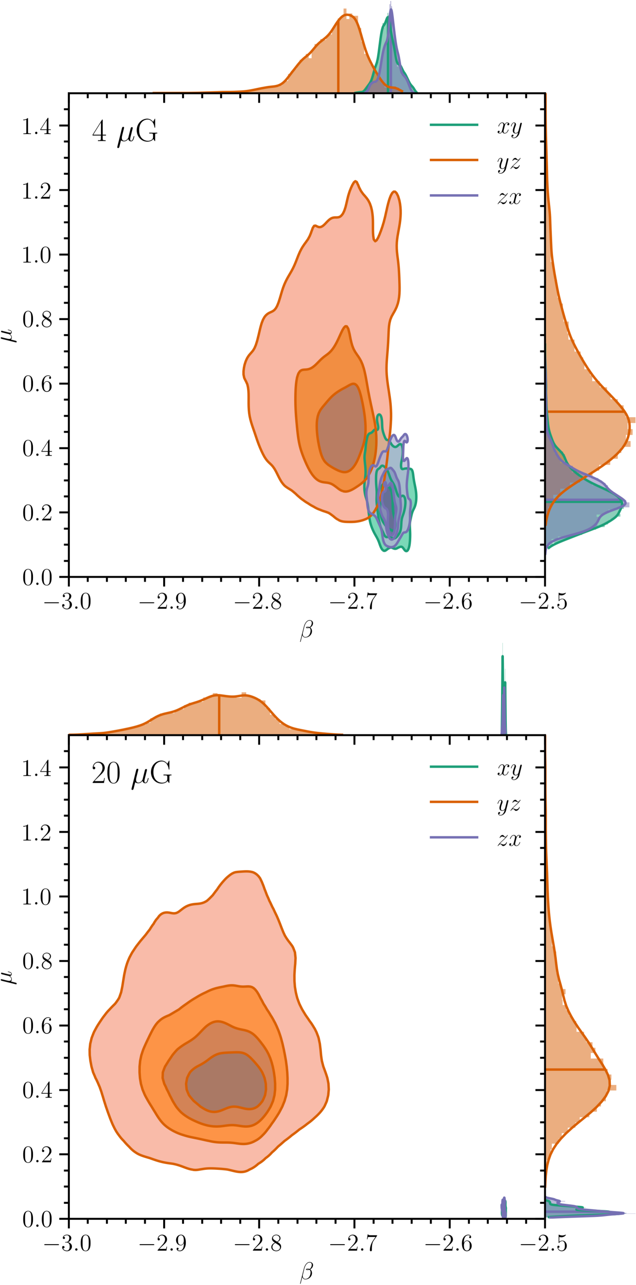
Figure 6: Bivariate distribution of the ratio between the standard deviation of $B_{\perp}$ and its median value, $\mu$, and the brightness temperature spectral index, $\beta$, computed in the frequency range 115$-$189 MHz for each LOS for the weak and strong field case (upper and lower panel, respectively), at a resolution of $6.7^{\prime}$. The POS are identified by the three different colours displayed in the legend. Isodensity contours are plotted at 5%, 30%, 50%, and 75% levels. The histograms above and to the right of the main plots show the marginal distribution of the two quantities. The median values are marked by horizontal and vertical lines and listed in Table 3.

4.3 Polarisation fraction

The local polarisation fraction, i.e., the polarisation fraction based on the local emissivities for an energy-independent value of $s$ is

$$p=\frac{3-3s}{7-3s}=\frac{3+3\beta}{1+3\beta}\,,$$ (10)

(see, e.g. Rybicki & Lightman, 1986), which, for $s=-2$ and $-3$, gives $p=69\%$ and 75%, respectively. If the orientation and the strength of ${\bf B}_{\perp}$ do not vary along the LOS, Eq. (10) would also give the polarisation fraction in the POS. To quantify the limitations of the above assumption, we calculate the expected polarisation fraction (Eq. (8)) at the reference frequency $\nu=130$ MHz for the two simulations and at the resolution of $6.7^{\prime}$ in the three POS. Similarly to Fig. 6, in Fig. 7 we show the results in the form of bivariate and marginal distributions, and we find a similar correlation of $\mu$ with $p$ as we found with $\beta$: as $\mu$ increases, the spread of values of $p$ around its median value is even larger than that of $\beta$ (see Table 3).

Furthermore, except for the POS $xy$ and $zx$ in the strong field case, the median value is much lower than the theoretical value of $\simeq 70\%$ of the local polarisation fraction, which is the maximum value of the observed polarisation fraction. Such depolarisation effect in our study is mainly caused by the tangling of the turbulent component of the magnetic field along the LOS. This effect has been extensively reported in the literature both in the radio (e.g., Gaensler et al., 2011) and in the sub-millimetre domain (e.g., Planck Collaboration Int. XX, 2015). Moreover, radio synchrotron polarisation can be severely affected by other mechanisms that drastically reduce the amount of detectable polarised emission, such as Faraday rotation and beam depolarisation (see, e.g., Sokoloff et al., 1998; Haverkorn et al., 2004). We note that Faraday rotation at a few hundred MHz cannot be neglected from an observational point of view. However, in this study we choose not to detail this process and to only focus on the emission mechanism of synchrotron radiation with an energy-dependent spectral slope. Faraday rotation will be the core of a follow-up paper that will dig into the complexity of the ionisation degree of the multiphase diffuse ISM, a key ingredient to correctly model the effect of Faraday rotation.

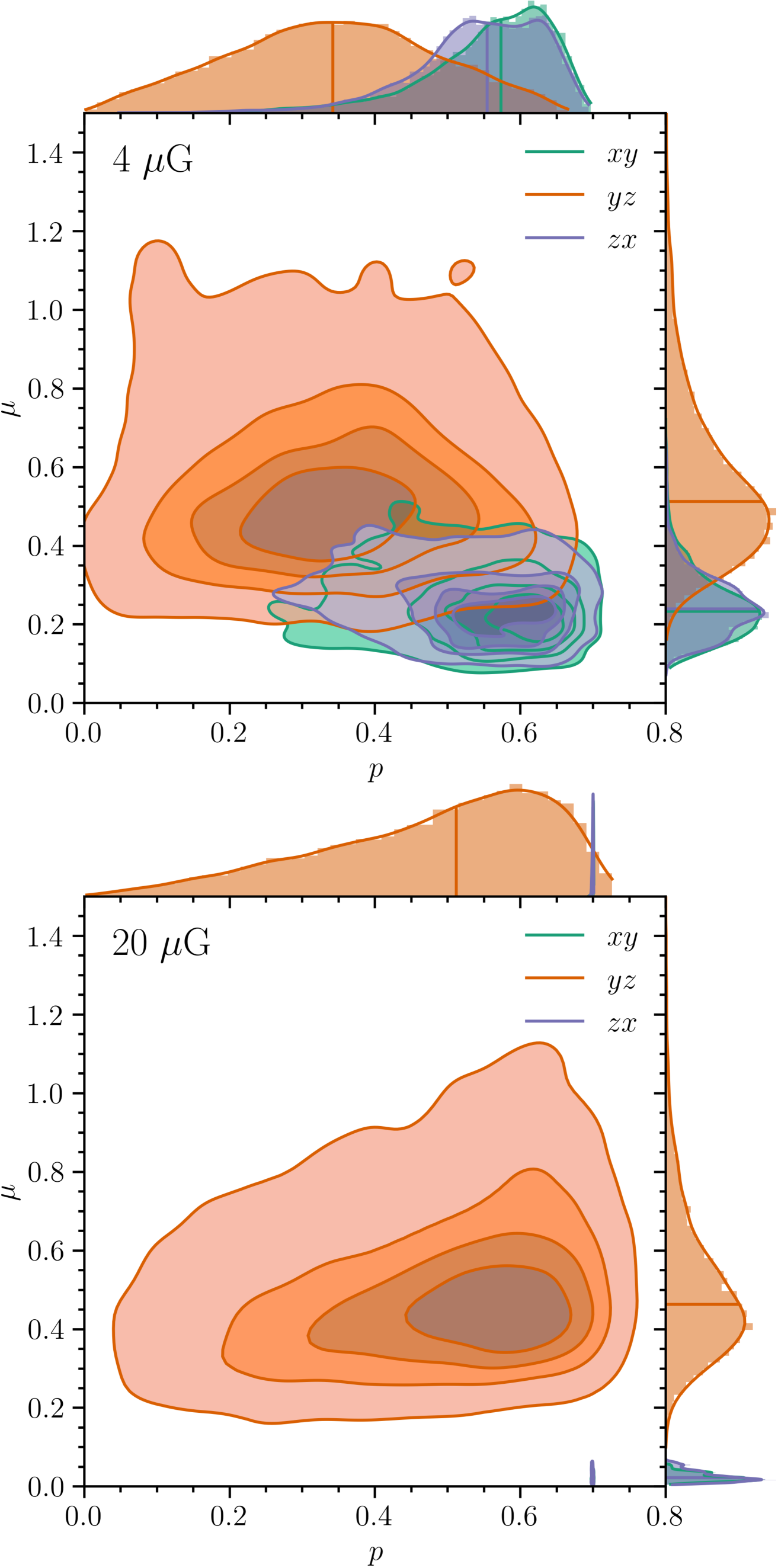
Figure 7: Bivariate distribution of the ratio between the standard deviation of $B_{\perp}$ and its median value, $\mu$, and the polarisation fraction, $p$, computed at 130 MHz for each LOS for the weak and strong field case (upper and lower panel, respectively), at a resolution of $6.7^{\prime}$. The POS are identified by the three different colours displayed in the legend. Isodensity contours are plotted at 5%, 30%, 50%, and 75% levels. The histograms above and to the right of the main plots show the marginal distribution of the two quantities. The median values are marked by horizontal and vertical lines and listed in Table 3.

5 Discussion

5.1 Effect of angular resolution on $\beta$ and $p$

In this study we have assumed the typical angular resolution of observations carried out with the most recent facilities, such as LOFAR. Here we show the distributions of the spectral index and the polarisation fraction obtained from lower resolution observations such as those shown in Guzmán et al. (2011). The latter paper presented an all-sky Galactic radio emission map, convolved to a common $5^{\circ}$ resolution, combining observations obtained with different telescopes such as the Parkes 64m, the Jodrell Bank MkI and MkIA, and the Effelsberg 100m (Haslam et al., 1981, 1982), the Maipú Radio Astronomy Observatory 45-MHz array (Alvarez et al., 1997), and the Japanese Middle and Upper atmosphere radar array (MU radar; Maeda et al., 1999). Figure 8 shows the comparison of the distributions of $\beta$ and $p$ (upper and lower panels, respectively) at the resolutions of $6.7^{\prime}$ and $5^{\circ}$ (filled and empty histograms, respectively). Despite the increase in resolution of LOFAR, the median value of $\beta$ does not change appreciably (see upper panels). However, what does change is the spread of the distribution, since at a lower resolution it is not possible to pick up the finer variations of the spectral index. More interesting is how the polarisation fraction distributions differ in the two cases. The lower panels show the beam depolarisation effect mentioned in Sect. 4.3: where $\mu$ is larger, a lower resolution clearly results in a lower $p$.

Figure 8: Histograms of the spectral index $\beta$ (upper panels) and polarisation fraction $p$ (lower panels) for the weak and strong field case (left and right column, respectively). Solid (empty) histograms refer to a resolution of $6.7^{\prime}$ ($5^{\circ}$). The POS are identified by the three different colours displayed in the legend.

5.2 A look-up plot for $B_{\perp}$

At any given position along a LOS, the synchrotron emission is jointly determined by the local CRe spectrum and the local value of $B_{\perp}$. As we showed in Sect. 3.1, thanks to the range of $\beta$ obtained from observations, it is possible to constrain the CRe spectrum at $\sim$GeV energies (see also Fig. 3). This makes it possible to reduce the uncertainly on the spectral shape, an appreciable improvement over the assumption of an energy-independent $s$. One should also consider that the latest generation of telescopes, such as LOFAR and in the near future SKA, reach resolutions up to at least three orders of magnitude higher than previous instruments. This means that the uncertainties on the values of $\beta$ derived from observations will be reduced and it will be possible to obtain $\beta$ variations over smaller fields of view. Finally, in Sect. 4.2 we showed that variations of $B_{\perp}$ along the LOS do not affect the estimates of $\beta$. This feature is particularly relevant for reducing the uncertainty in the estimation of the average value of $B_{\perp}$ along a LOS. Given these premises, we suggest a method for estimating $\langle B_{\perp}\rangle$, the average value of $B_{\perp}$, along a given LOS.

We adopt the Orlando (2018) CRe spectrum and assume $\nu$ in the range 10 MHz$-$20 GHz and $\langle B_{\perp}\rangle$ in the range 0.5$-$30 $\mu$G. We compute the corresponding emissivities (see Eqs. (1)), integrated along the LOS for 1 pc, and compute $\beta(\nu,\langle B_{\perp}\rangle)=d\log T_{\nu}(\langle B_{\perp}\rangle)/d\log\nu$. By inverting the relation for $\beta$, in Fig. 9 we show the values of $\langle B_{\perp}\rangle$ expected for each couple $(\nu,\beta)$.

We then consider three different ranges of frequencies: 115$-$189 MHz with a resolution of 183 kHz, 467$-$672 MHz with a resolution of 507 kHz, and 833$-$1200 MHz with a resolution of 908 kHz, labelled in Fig. 9 as low ($\mathcal{L}$), mid ($\mathcal{M}$), and high ($\mathcal{H}$) frequency range, respectively. Following the procedure described in Sect. 4.2, for each POS of the two snapshots, we calculate the temperature maps as a function of frequency at a resolution of $6.7^{\prime}$ and we extract the $\beta$ value for each LOS and for each of the three frequency intervals, $\mathcal{L}$, $\mathcal{M}$, and $\mathcal{H}$, by a linear fit of $\log T_{\nu}$ versus $\log\nu$. We show in Fig. 9 the $\tilde{\beta}$ values for each POS by estimating the errors using the first and third quartiles for each frequency interval. We note that, since the POS $xy$ and $zx$ for both snapshots have the same $\tilde{\beta}$, in the figure we show four values instead of six. The values of $\tilde{\beta}$ for the $\mathcal{L}$ frequency range are listed in Table 3, while those for the $\mathcal{M}$ and $\mathcal{H}$ ranges are reported in Table 4.

Figure 9: A look-up plot to estimate the average value of $B_{\perp}$ along a LOS, $\langle B_{\perp}\rangle$, for a given frequency $\nu$ and brightness temperature spectral index $\beta$ assuming the CRe spectrum by Orlando (2018). Black and white isocontours show specific values of $\langle B_{\perp}\rangle$ with labels in $\mu$G. Yellow symbols indicate estimates of $\langle B_{\perp}\rangle$ obtained from the values of $\tilde{\beta}$ in the frequency ranges 115$-$189 MHz, 467$-$672 MHz, and 833$-$1200 MHz (labelled as $\mathcal{L}$, $\mathcal{M}$, and $\mathcal{H}$, respectively), at a common resolution of $6.7^{\prime}$, for the different POS of the two simulation snapshots (circles: POS $yz$ in the strong field case; squares: POS $yz$ in the weak field case; diamonds: POS $xy$ and $zx$ in the weak field case; triangles: POS $xy$ and $zx$ in the strong field case). Rectangles at the bottom of the plot show the frequency ranges of the low and high band antenna of LOFAR (LBA and HBA, respectively), the low and mid frequency bands of SKA (SKA1-Low and SKA1-Mid, respectively), and SKA pathfinders and precursors: the Hydrogen Epoch or Reionisation (HERA); the Murchison Widefield Array (MWA); the Karoo Array Telescope (MeerKAT); the Australian SKA Pathfinder (ASKAP).

Figure 9 shows that, for each POS, the estimates of $\tilde{\beta}$ in the three frequency intervals correspond to the same $\langle B_{\perp}\rangle$, which also agree with the respective value of $\tilde{B}_{jk}$ listed in Table 1. This confirms the consistency of our procedure.

This plot shows that there is a preferred range of frequencies that can be conveniently used to estimate $\langle B_{\perp}\rangle$ along a LOS. This range corresponds approximately to 100 MHz$-$5 GHz, the frequency interval where $s$, and hence $\beta$, varies the most and where the isocontours of $\langle B_{\perp}\rangle$ are more separated. Conversely, at frequencies that are too low (high), the CRe spectrum flattens out if $\langle B_{\perp}\rangle$ is too high (low), and the estimate of $\langle B_{\perp}\rangle$ becomes more uncertain. From this figure it can be concluded that, in order to have a more precise estimate of $\langle B_{\perp}\rangle$, it is advisable to simultaneously observe in narrow frequency ranges with high spectral resolution (as our $\mathcal{L}$, $\mathcal{M}$, and $\mathcal{H}$ intervals) in order to have independent $\beta$ estimates that should follow a specific isocontour of $B_{\perp}$.

6 Summary

We carried out a quantitative study to understand the consequences of an energy-dependent CRe spectral slope in the interpretation of observations of synchrotron emission in the diffuse and magnetised ISM. We focused in particular on metre wavelengths that can currently be observed with state-of-the-art facilities such as LOFAR and in the near future with SKA. At frequencies lower (higher) than $\simeq 400$ MHz a constant spectral slope $s=-2$ ($s=-3$) is often assumed, mainly to avoid time-consuming calculations in analytical models and numerical simulations. As a consequence, one should also expect a constant value for the brightness temperature spectral index, $\beta$, related to $s$ by $\beta=(s-3)/2$ (Rybicki & Lightman, 1986). However, metre wavelength observations show that $\beta$ is not constant across the Galaxy, taking on values quite different from $-2.5$ (corresponding to $s=-2$), varying between about $-2.7$ and $-2.1$ (Guzmán et al., 2011).

For typical magnetic field strengths expected in the diffuse ISM ($\simeq 2-20\leavevmode\nobreak\ \mu$G), the electrons that mostly determine the synchrotron emission at frequencies between about 100 MHz and 10 GHz have energies in the range $\simeq$100 MeV$-$50 GeV. It is precisely at these energies that the spectral slope shows the largest variations. For example, for the CRe spectrum described in Orlando (2018), representative of intermediate Galactic latitudes including most of the local emission within about 1 kpc around the Sun, in this energy range $s$ varies between about $-3.2$ and $-1.8$.

In order to understand the effect of an energy-dependent spectral slope at a quantitative level, we first considered a slab with a fixed, spatially uniform $B_{\perp}$ exposed to a flux of CRe and we showed that, thanks to high-precision observational estimates of $\beta$ at low frequencies (Mozdzen et al., 2017), it is possible to discard some realisations of the CRe spectrum that would imply unrealistically high values of $B_{\perp}$. Then, we used two snapshots of 3D MHD simulations (Bellomi et al., 2020) with different median magnetic field strength, and studied the synchrotron emission according to the CRe spectrum by Orlando (2018). We computed the distribution of $\beta$ for three frequency ranges, at low, mid, and high frequencies (115$-$189 MHz, 467$-$672 MHz, and 833$-$1200 MHz, respectively). We showed that the assumption of an energy-independent $s$ is not justified and leads to non-negligible biases in the interpretation of the observed spectral index distributions. In particular, we found that $\beta$ becomes less negative as $B_{\perp}$ increases and that the dispersion of the distribution of spectral index values around its median weakly depends on how much $B_{\perp}$ varies along the LOS. This property is of special relevance since, once a CRe spectrum is assumed, the uncertainty about the expected average value of $B_{\perp}$for a given LOS, $\langle B_{\perp}\rangle$, is reduced. We then presented a look-up plot that makes it possible to estimate $\langle B_{\perp}\rangle$ given $\beta$ values obtained from observations in one or more frequency intervals. More precisely, we suggest repeating observations in narrow frequency intervals with high spectral resolution in order to have independent estimates of $\beta$ that should lie on the same $\langle B_{\perp}\rangle$ isocontour in the look-up plot.

Finally, we computed the expected polarisation fraction, $p$, finding that it is expected to be smaller the more turbulent the magnetic field along the LOS is, deviating noticeably from the maximum value of $\simeq 70\%$. The dispersion of $p$ around its median value is larger than that of $\beta$ as a consequence of the turbulent tangling of the magnetic field lines along the LOS. The analysis of this depolarisation effect and the consequences of Faraday rotation are deferred to a subsequent paper.

Appendix A Bivariate distributions of $\mu$ and $\beta$ at high frequencies

Following the procedure outlined in Sect. 4.2, we consider two higher frequency ranges, 467$-$672 MHz and 833$-$1200 MHz (labelled $\mathcal{M}$ and $\mathcal{H}$, respectively), for the calculation of $\beta$ in the three POS of the two simulation snapshots. Figure 10 shows the bivariate distribution of $\mu$ and $\beta$ for these two frequency ranges, comparing them with the distribution for the range 115$-$189 MHz (labelled $\mathcal{L}$) described in Sect. 4.2. In order to increase clarity and to avoid overlapping distributions, we only show density isodensity contours plotted at 50% and 80%. As the frequency range increases, the $\beta$ distributions shift towards more negative values. This can be explained by looking at Fig. 3 where we see that as the frequency increases, the energies determining the synchrotron emissivity are higher and higher. Higher energies correspond to more negative values of $s$, and therefore of $\beta$. For completeness, Table 4 shows the values of $\tilde{\beta}$ for the three POS of the two snapshots considered in the frequency intervals $\mathcal{M}$ and $\mathcal{H}$.

Figure 10: Bivariate distribution of the ratio between the standard deviation of $B_{\perp}$ and its median value, $\mu$, and the brightness temperature spectral index, $\beta$, computed in the frequency ranges 115$-$189 MHz, 467$-$672 MHz, and 833$-$1200 MHz (labelled $\mathcal{L}$, $\mathcal{M}$, and $\mathcal{H}$, respectively) for each LOS for the weak and strong field case (left and right panel, respectively), at a resolution of $6.7^{\prime}$. The POS are identified by the three different colours displayed in the legend. Isodensity contours are plotted at 50% and 80%.

Table 4: Medians of the brightness temperature spectral index for the three POS and the two cases of weak and strong field at a resolution of $6.7^{\prime}$. Labels $\mathcal{M}$ and $\mathcal{H}$ identify the frequency intervals 467$-$672 MHz and 833$-$1200 MHz, respectively^a.

	POS	$\tilde{\beta}$
		$\mathcal{M}$	$\mathcal{H}$
weak field ($B_{0}=4\leavevmode\nobreak\ \mu$G)	$xy$	$-2.83\pm 0.01$	$-2.92\pm 0.01$
	$yz$	$-2.89\pm 0.02$	$-2.98\pm 0.02$
	$zx$	$-2.83\pm 0.01$	$-2.92\pm 0.01$
strong field ($B_{0}=20\leavevmode\nobreak\ \mu$G)	$xy$	$-2.65$	$-2.72$
	$yz$	$-3.02\pm 0.03$	$-3.08\pm 0.02$
	$zx$	$-2.65$	$-2.72$

^a  Errors have been estimated using the first and third quartiles. Errors smaller than 0.01 are not shown.

Appendix B Brightness temperature spectral index maps

Here we show the spectral index maps obtained for the two simulations described in Sect. 3.2. These maps have been derived considering the same frequency range and frequency resolution of LOFAR observations by Jelić et al. (2015), namely $\nu=115-189$ MHz and $\Delta\nu=183$ kHz, respectively. In the POS where $\mu\ll 1$, namely the $xy$ and $zx$ POS of the strong field case, $\beta$ shows a constant value. Then, the greater the turbulent component of the field, the greater the variations that $\beta$ exhibits on small scales. The latter can in principle be resolved by observations with LOFAR. From these maps, the histograms displayed in Fig. 6 were produced.

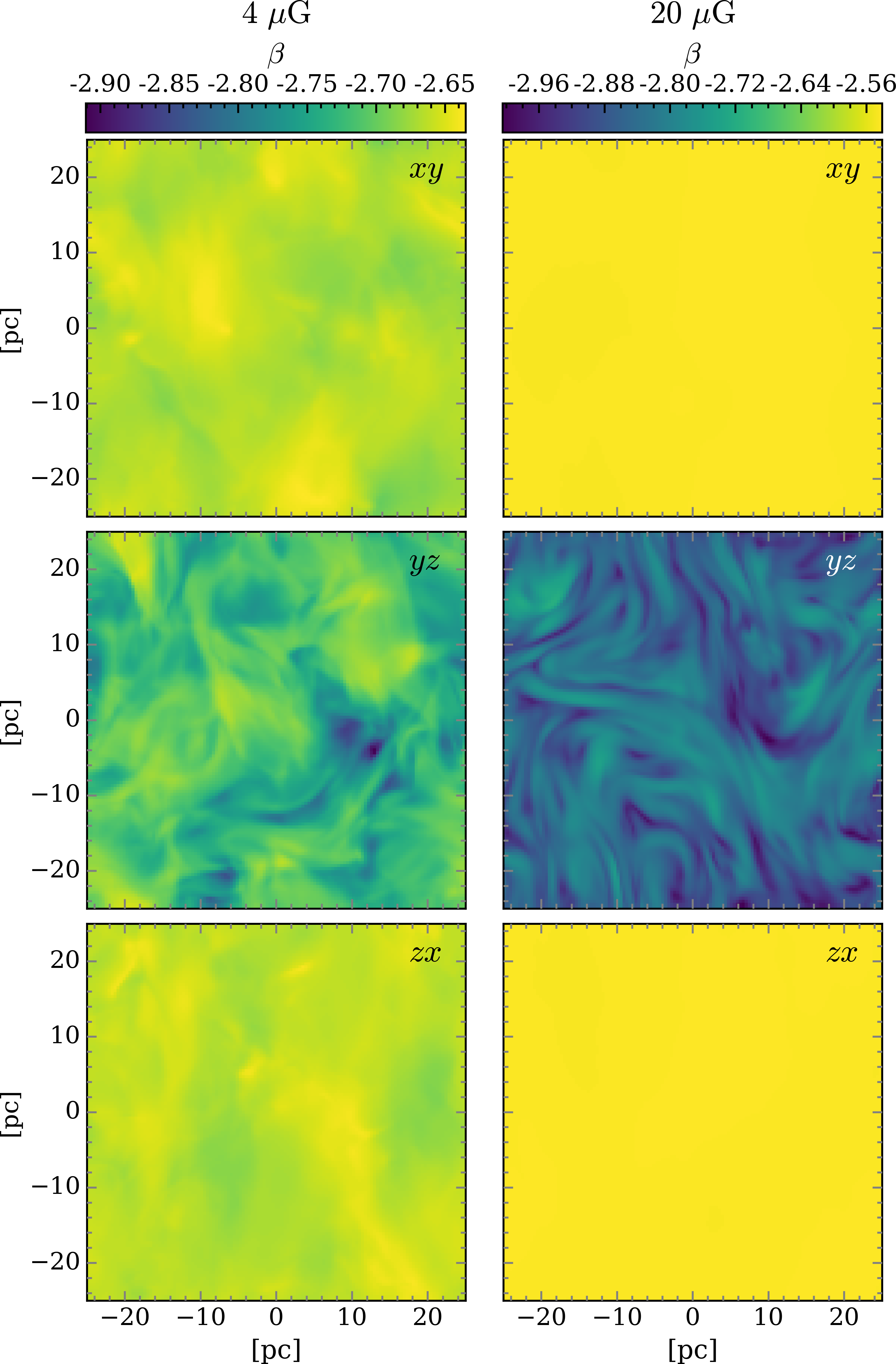
Figure 11: Brightness temperature spectral index maps for the three POS (three rows) of the weak and strong field case (left and right column, respectively) for a resolution of $6.7^{\prime}$. The three panels of each column share the same colourbar on the top.