The weak convergence order of two Euler-type discretization schemes for the log-Heston model

Annalena Mickel 111Mathematical Institute and DFG Research Training Group 1953, University of Mannheim, B6, 26, D-68131 Mannheim, Germany, amickel@mail.uni-mannheim.de โ€ƒโ€ƒ Andreas Neuenkirch 222Mathematical Institute, University of Mannheim, B6, 26, D-68131 Mannheim, Germany, aneuenki@mail.uni-mannheim.de
Abstract

We study the weak convergence order of two Euler-type discretizations of the log-Heston Model where we use symmetrization and absorption, respectively, to prevent the discretization of the underlying CIR process from becoming negative. If the Feller index $\nu$ of the CIR process satisfies $\nu>1$, we establish weak convergence order one, while for $\nu\leq 1$, we obtain weak convergence order $\nu-\epsilon$ for $\epsilon>0$ arbitrarily small. We illustrate our theoretical findings by several numerical examples.

Key words: Heston model, CIR process, discretization schemes for SDEs, Kolmogorov PDE, Euler scheme, non-standard assumptions
2010 Mathematics Subject Classification: 60H35; 65C05; 65C30; 91G60

1 Introduction and Main Result

The Heston model [24] is given by the stochastic differential equation (SDE)

$\displaystyle\begin{split}dS_{t}&=\mu S_{t}dt+\sqrt{V_{t}}S_{t}\Big{(}\rho dW_{t}+\sqrt{1-\rho^{2}}dB_{t}\Big{)},\qquad&S_{0}=s_{0},\\ dV_{t}&=\kappa(\theta-V_{t})dt+\sigma\sqrt{V_{t}}dW_{t},\qquad\qquad\qquad\qquad\,\,&V_{0}=v_{0},\end{split}$ (1)

with s0,v0,ฮบ,ฮธ,ฯƒ>0subscript๐‘ 0subscript๐‘ฃ0๐œ…๐œƒ๐œŽ0s_{0},v_{0},\kappa,\theta,\sigma>0, $\mu\in\mathbb{R}$, $\rho\in[-1,1]$, $T>0$ and independent Brownian motions $W=(W_{t})_{t\in[0,T]}$, $B=(B_{t})_{t\in[0,T]}$ which are defined on a filtered probability space $(\Omega,\mathcal{F},(\mathcal{F}_{t})_{t\in[0,T]},\mathbb{P})$ where the filtration satisfies the usual conditions. Throughout this article the initial values s0subscript๐‘ 0s_{0}, $v_{0}$ are assumed to be deterministic. Here, $S$ models the price of an asset and $V$ its volatility which is given by the so called Coxโ€“Ingersollโ€“Ross process (CIR).

The Heston model extends the celebrated Black-Scholes model by using a stochastic volatility instead of a constant one. Its numerical analysis is not only of theoretical relevance. With the recent rise of volatility trading in financial markets, stochastic volatility models as the Heston model are becoming more and more important and numerical calculations are essential for the practical use of these models.

To price options with maturity at time $T$ and discounted payoff function $g:[0,\infty)\rightarrow\mathbb{R}$, one is interested in the value of

$\displaystyle\mathbb{E}\left[g(S_{T})\right],$

which can be approximated through a (multi-level) Monte Carlo simulation. Usually, the log-Heston model instead of the Heston model is considered in numerical practice. With $X_{t}=\log(S_{t})$ this yields the SDE

$\displaystyle\begin{split}dX_{t}&=\Big{(}\mu-\frac{1}{2}V_{t}\Big{)}dt+\sqrt{V_{t}}\Big{(}\rho dW_{t}+\sqrt{1-\rho^{2}}dB_{t}\Big{)},\\ dV_{t}&=\kappa(\theta-V_{t})dt+\sigma\sqrt{V_{t}}dW_{t},\end{split}$ (2)

and the exponential is then incorporated in the payoff, i.e.ย g๐‘”g is replaced by $h:\mathbb{R}\rightarrow\mathbb{R}$ with $h(x)=g(\exp(x))$.

Note that the state space of the log-Heston SDE (2) is $\mathbb{R}\times[0,\infty)$ and the square-root coefficients are not globally Lipschitz continuous. Additionally, even if $g$ satisfies a linear growth condition, $g(S_{T})$ might not belong to $L^{p}$ if $p>1$. See e.g. [7] for this so-called moment explosion. Thus, the (log-)Heston SDE does not satisfy the standard assumptions for the numerical analysis of SDEs.

Due to its popularity and its difficulty various methods for the simulation of the (log-)Heston model have been proposed and studied:

  • (i)

    exact simulations schemes which are based on the transition density of the CIR process and the characteristic function of the log-asset price process, see e.g. [14, 37, 20, 31, 21, 30],

  • (ii)

    semi-exact discretization schemes which simulate the CIR process exactly, but discretize the log-asset price, see e.g. [6, 39, 32],

  • (iii)

    full discretization schemes which discretize both components of the SDE, see e.g. [25, 26, 6, 35, 34, 36, 5],

  • (iv)

    and miscellaneous methods as e.g. tree methods in [1, 16] or the moment matching methods in [6].

Euler-type discretization schemes are frequently used for the log-Heston model and seem to be efficient in many cases, but a weak error analysis, i.e. an analysis of the bias of these discretization schemes, is not available yet. Since the discretization of the CIR process might become negative, these schemes require fixes as absorption and symmetrization or a modification of the square-root coefficient for negative values which make these schemes applicable but their analysis even more challenging. For a survey of such fixes and modifications see e.g. [36]. Moreover, for the importance of the weak error in (multi-level) Monte Carlo simulations see [17] and [19].

Here, we will use two of these schemes for the discretization of the CIR component. The Symmetrized Euler (SE) scheme given by

vk+1sโ€‹yโ€‹msubscriptsuperscript๐‘ฃ๐‘ ๐‘ฆ๐‘š๐‘˜1\displaystyle v^{sym}_{k+1} =|vksโ€‹yโ€‹m+ฮบโ€‹(ฮธโˆ’vksโ€‹yโ€‹m)โ€‹(tk+1โˆ’tk)+ฯƒโ€‹vksโ€‹yโ€‹mโ€‹(Wtk+1โˆ’Wtk)|,absentsubscriptsuperscript๐‘ฃ๐‘ ๐‘ฆ๐‘š๐‘˜๐œ…๐œƒsubscriptsuperscript๐‘ฃ๐‘ ๐‘ฆ๐‘š๐‘˜subscript๐‘ก๐‘˜1subscript๐‘ก๐‘˜๐œŽsubscriptsuperscript๐‘ฃ๐‘ ๐‘ฆ๐‘š๐‘˜subscript๐‘Šsubscript๐‘ก๐‘˜1subscript๐‘Šsubscript๐‘ก๐‘˜\displaystyle=\biggl{|}v^{sym}_{k}+\kappa\left(\theta-v^{sym}_{k}\right)(t_{k+1}-t_{k})+\sigma\sqrt{v^{sym}_{k}}\left(W_{t_{k+1}}-W_{t_{k}}\right)\biggr{|}, (3)

where $0=t_{0}<t_{1}<...<t_{k}<...<t_{N}=T$ and v0sโ€‹yโ€‹m=v0subscriptsuperscript๐‘ฃ๐‘ ๐‘ฆ๐‘š0subscript๐‘ฃ0v^{sym}_{0}=v_{0}, has been proposed and studied by Bossy and Diop in [12]. They state the weak convergence order one (for sufficiently regular test functions) under the assumption $\frac{\kappa\theta}{\sigma^{2}}>1$ for this scheme. Instead of reflecting negative values, the Euler scheme with absorption or Absorbed Euler (AE) scheme sets all occurring negative values of the CIR discretization to zero, i.e.

vk+1aโ€‹bโ€‹s=(vkaโ€‹bโ€‹s+ฮบโ€‹(ฮธโˆ’vkaโ€‹bโ€‹s)โ€‹(tk+1โˆ’tk)+ฯƒโ€‹vkaโ€‹bโ€‹sโ€‹(Wtk+1โˆ’Wtk))+subscriptsuperscript๐‘ฃ๐‘Ž๐‘๐‘ ๐‘˜1superscriptsubscriptsuperscript๐‘ฃ๐‘Ž๐‘๐‘ ๐‘˜๐œ…๐œƒsubscriptsuperscript๐‘ฃ๐‘Ž๐‘๐‘ ๐‘˜subscript๐‘ก๐‘˜1subscript๐‘ก๐‘˜๐œŽsubscriptsuperscript๐‘ฃ๐‘Ž๐‘๐‘ ๐‘˜subscript๐‘Šsubscript๐‘ก๐‘˜1subscript๐‘Šsubscript๐‘ก๐‘˜v^{abs}_{k+1}=\left(v^{abs}_{k}+\kappa\left(\theta-v^{abs}_{k}\right)(t_{k+1}-t_{k})+\sigma\sqrt{v^{abs}_{k}}\left(W_{t_{k+1}}-W_{t_{k}}\right)\right)^{+} (4)

and v0aโ€‹bโ€‹s=v0subscriptsuperscript๐‘ฃ๐‘Ž๐‘๐‘ 0subscript๐‘ฃ0v^{abs}_{0}=v_{0}. Its exact origin is unknown and also no weak convergence rates are known for it. Using SE or AE, we then discretize the log-price process with the standard Euler method:

$$x_{k+1}=x_{k}+\Big{(}\mu-\frac{1}{2}v_{k}\Big{)}(t_{k+1}-t_{k})+\sqrt{v_{k}}\Big{(}\rho\left(W_{t_{k+1}}-W_{t_{k}}\right)+\sqrt{1-\rho^{2}}\left(B_{t_{k+1}}-B_{t_{k}}\right)\Big{)}.$$ (5)

We will work with an equidistant discretization

$$t_{k}=k\Delta t,\quad k=0,\ldots,N,$$

with $\Delta t=T/N$ and $N\in\mathbb{N}$. Moreover, we will use the standard notations for the spaces of differentiable functions. In particular, the subscript $pol$ denotes polynomial growth. See also Subsection 3.1. Finally, we set

$$\nu=\frac{2\kappa\theta}{\sigma^{2}},$$

i.e. $\nu$ is the Feller index of the CIR process $V=(V_{t})_{t\in[0,T]}$.

Our analysis leads us to the following theorem:

Theorem 1.1.

(i) Let $f\in C^{6}_{pol}(\mathbb{R}\times[0,\infty))$ and $\nu>1$. Then both schemes satisfy

$\displaystyle\limsup\limits_{N\rightarrow\infty}\,\frac{\left|\mathbb{E}\left[f(x_{N},v_{N})\right]-\mathbb{E}\left[f(X_{T},V_{T})\right]\right|}{\left|T/N\right|}<\infty.$

(ii) Let $f\in C^{6}_{pol}(\mathbb{R}\times[0,\infty))$ and $\nu\leq 1$. Then both schemes satisfy

$\displaystyle\limsup\limits_{N\rightarrow\infty}\,\frac{\left|\mathbb{E}\left[f(x_{N},v_{N})\right]-\mathbb{E}\left[f(X_{T},V_{T})\right]\right|}{\left|T/N\right|^{\alpha}}=0$

for all $\alpha\in(0,\nu)$.

Thus, for $\nu>1$ we have weak convergence order one and for $\nu\leq 1$ we have weak convergence order $\nu-\epsilon$ for arbitrarily small $\epsilon>0$. In view of these convergence rates, exact and semi-exact simulation schemes are relevant alternatives for small Feller indices $\nu$.

Remark 1.2.

Our analysis builds on the regularity of the Heston PDE established in [13]. Moreover, we use the local time-approach for the analysis of the discretization of the CIR process from [12] and we modify and improve the analysis of the probability that the discretization of the CIR process becomes negative from [12, 15]. In particular, we are able to remove the restriction $\nu>2$ for the Feller index in comparison to [12, 15].

As already mentioned, [12] studies the weak error of the symmetrized Euler scheme for the CIR process. In [15] the strong error of a fully truncated Euler scheme for the CIR process is analyzed, while [13] studies a hybrid-tree scheme for option pricing in stochastic volatility models with jumps.

Remark 1.3.

The (positivity preserving) weak approximation of the CIR process has been also studied by Alfonsi in [2, 3]. In particular, weak first and second order schemes have been derived in these references. The weak approximation of the log-Heston model by a combined Euler scheme for $X_{t}$ and a drift implicit Milstein scheme for $V_{t}$ has been studied in [4, 5]. In these works weak convergence order one is obtained for smooth test functions $f$ if $\nu>2$ and for bounded and measurable test functions $f$ if $\nu>\frac{9}{2}$, respectively.

Another approach for the weak approximation of the CIR process and the Heston model, which combines the cubature on Wiener space approach and the classical Runge-Kutta method for ordinary differential equations, has been introduced in [34]; see also the related work [35] and Remark 2.2.

Remark 1.4.

A decay of the weak convergence rate for $\nu<1$ has also been numerically observed in [14] for an Euler scheme for the Heston Model and for some of the schemes in [2] for the CIR process. Interestingly, the convergence order $\nu$ also appears for the CIR process in a different context, namely for the $L^{1}$-approximation at the terminal time point. If $\nu<1$, then $\nu$ is the best possible convergence order that arbitrary approximations based on an equidistant discretization of the driving Brownian motion can achieve, see [23]. Together with [22] and [33] the latter reference also provides a comprehensive survey on the strong approximation of the CIR process.

Remark 1.5.

The Heston model was introduced in the 1990s and is now a classical stochastic volatility model; our analysis addresses a problem that has been open for a long time. Meanwhile, the Heston model has been extended in several ways, e.g., by adding jumps [9, 13] or by considering rough volatility processes instead of the CIR process, which leads to the rough Bergomi model [10] or the rough Heston model [18].


2 Numerical results

In this section, we will test numerically whether the weak convergence rates of Theorem 1.1 are attained even under milder assumptions on the test function $f$. We will consider a call, a put and a digital option. These payoffs are at most Lipschitz continuous which is typical in financial applications. This lack of smoothness is in contrast to the usual assumptions on $f$ for a weak error analysis. See also Remark 2.2.

We use the following model parameters.

  1. Model 1:

    $S_{0}=100,V_{0}=0.04,K=100,\kappa=5,\theta=0.04,\sigma=0.61,\rho=-0.7,T=1,r=0.0319$

  2. Model 2:

    $S_{0}=100,V_{0}=0.0457,K=100,\kappa=5.07,\theta=0.0457,\sigma=0.48,\rho=-0.767,T=2,r=0.0$

  3. Model 3:

    $S_{0}=100,V_{0}=0.010201,K=100,\kappa=6.21,\theta=0.019,\sigma=0.61,\rho=-0.7,T=1,r=0.0319$

  4. Model 4:

    $S_{0}=100,V_{0}=0.09,K=100,\kappa=2,\theta=0.09,\sigma=1,\rho=-0.3,T=5,r=0.05$

With these examples, we try to cover a wide range of Feller indices. We have $\nu\approx 1.075$ in Model 1, $\nu\approx 2.01$ in Model 2, $\nu\approx 0.63$ in Model 3 and $\nu\approx 0.36$ in Model 4. For each model, we use the following discounted payoff functions:

  1. 1.

    European call: $g_{1}(S_{T})=e^{-rT}\max\{S_{T}-K,0\}$

  2. 2.

    European put: $g_{2}(S_{T})=e^{-rT}\max\{K-S_{T},0\}$

  3. 3.

    Digital option: $g_{3}(S_{T})=e^{-rT}\mathbbm{1}_{[0,K]}(S_{T})$

Note that none of these payoffs satisfies the assumption of our Theorem. Thus, numerical convergence rates which coincide with the rates of our Theorem indicate that the latter might be valid under milder assumptions.

In order to measure the weak error rate, we simulated $M=2\cdot 10^{7}$ independent copies giโ€‹(sN(j))subscript๐‘”๐‘–superscriptsubscript๐‘ ๐‘๐‘—g_{i}(s_{N}^{(j)}), $j=1,\ldots,M$, of giโ€‹(sN)subscript๐‘”๐‘–subscript๐‘ ๐‘g_{i}\left(s_{N}\right) with sN=expโก(xN)subscript๐‘ ๐‘subscript๐‘ฅ๐‘s_{N}=\exp(x_{N}) to estimate

๐”ผโ€‹(giโ€‹(sN))๐”ผsubscript๐‘”๐‘–subscript๐‘ ๐‘\mathbb{E}(g_{i}(s_{N}))

by

pM,N=1Mโ€‹โˆ‘j=1Mgiโ€‹(sN(j))subscript๐‘๐‘€๐‘1๐‘€superscriptsubscript๐‘—1๐‘€subscript๐‘”๐‘–superscriptsubscript๐‘ ๐‘๐‘—p_{M,N}=\frac{1}{M}\sum_{j=1}^{M}g_{i}(s_{N}^{(j)})

for each combination of model parameters, payoff and number of steps $N\in\{2^{3},...,2^{7}\}$ or $N\in\{2^{3},...,2^{8}\}$ where $\Delta t=\frac{T}{N}$. To obtain a stable estimate of the convergence rates, we started with a $\Delta t$ which is roughly around $\frac{1}{\kappa}$ (which is required also for some auxiliary results of the proof of our main result). The Monte Carlo mean of these samples is then compared to a reference solution $p_{\sf ref}$, i.e.,

$$e(N)=|p_{\sf ref}-p_{M,N}|,$$

and we measure the weak error order by the slope of a least-squares fit of the data $(N,\log_{2}(e(N))$. The reference solutions can be computed with sufficiently high accuracy from semi-explicit formulae via Fourier methods. In particular, the put price can be calculated from the call pricing formula given in [24] via the put-call-parity. The price of the digital option can be computed from the probability $P_{2}$ given in [24]; it equals $e^{-rT}\left(1-P_{2}\right)$.

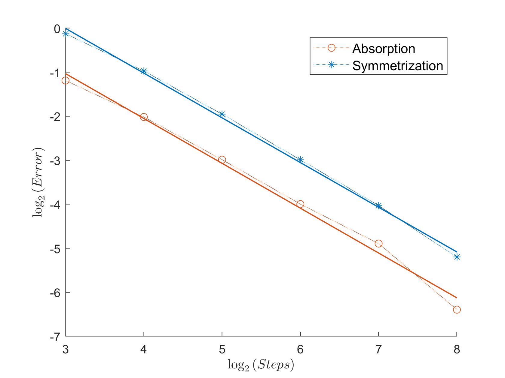
In Table 1 we can see the measured convergence rates for Model 1. In Figure 1, the error plot for the call option is displayed333The plots for the different options behave similarly, i.e. regularly and in accordance with Theorem 1.1, so we show only one plot for each option..

Method Call Put Digital
SE 1.02 1.00 0.94
AE 1.02 0.94 0.91
Table 1: Measured convergence rates Model 1

Because of our results in Theorem 1.1, we would expect SE and AE to have a weak convergence rate of $1$ and this is indeed the case in this example.

Refer to caption
Figure 1: Call Model 1

Looking at the plot, we can see that the convergence behavior is very regular.

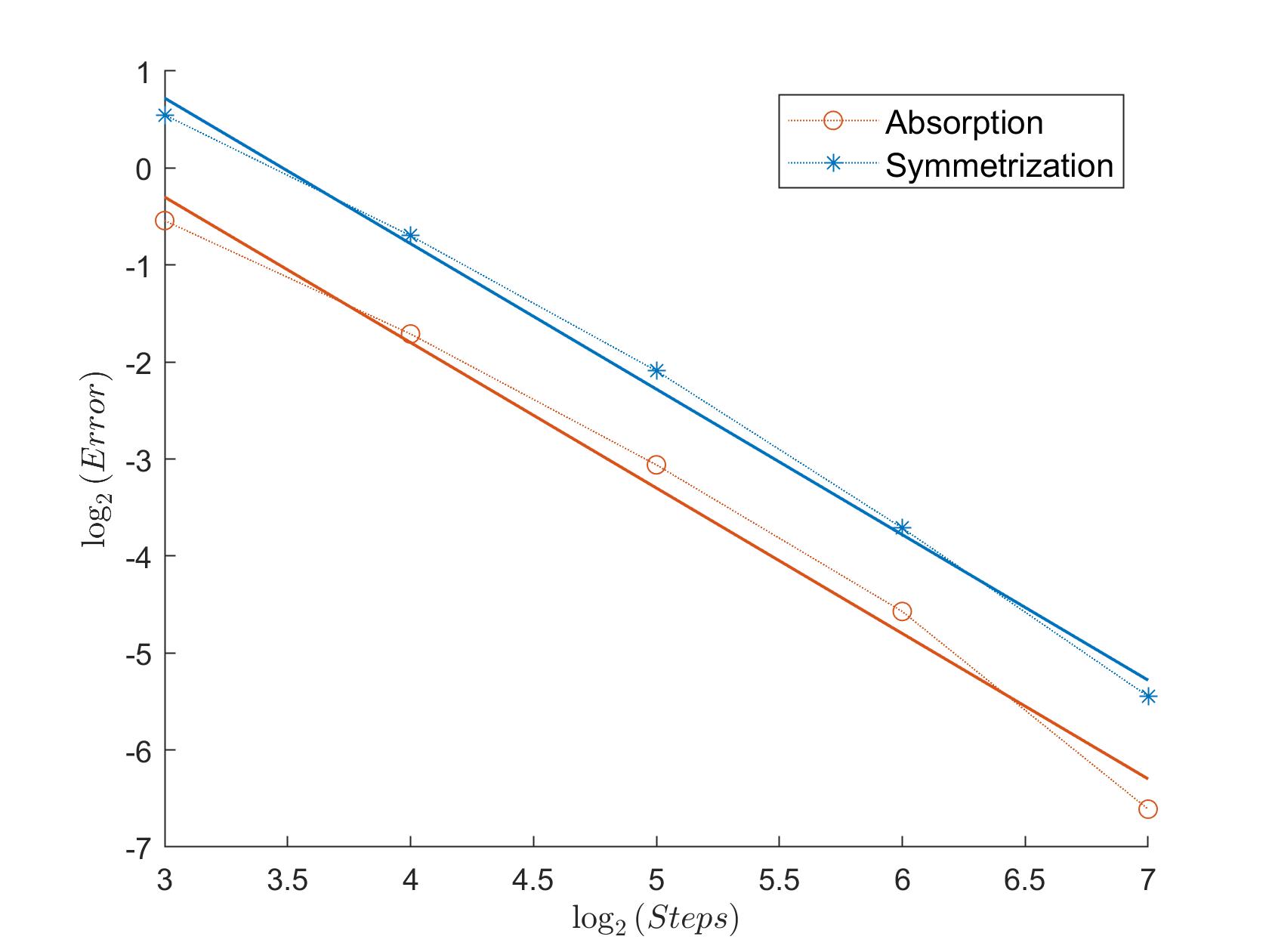
For the next model, we would again expect a convergence rate around $1$. The results from Table 2 indicate that for particular payoffs even a higher numerical rate is obtained if the Feller index is larger than $1$. The rates of SE and AE are around $1.5$. The error plot of the put option in Figure 2 shows again a regular convergence behavior.

Method Call Put Digital
SE 1.51 1.50 1.34
AE 1.37 1.50 1.42
Table 2: Measured convergence rates Model 2
Refer to caption
Figure 2: Put Model 2

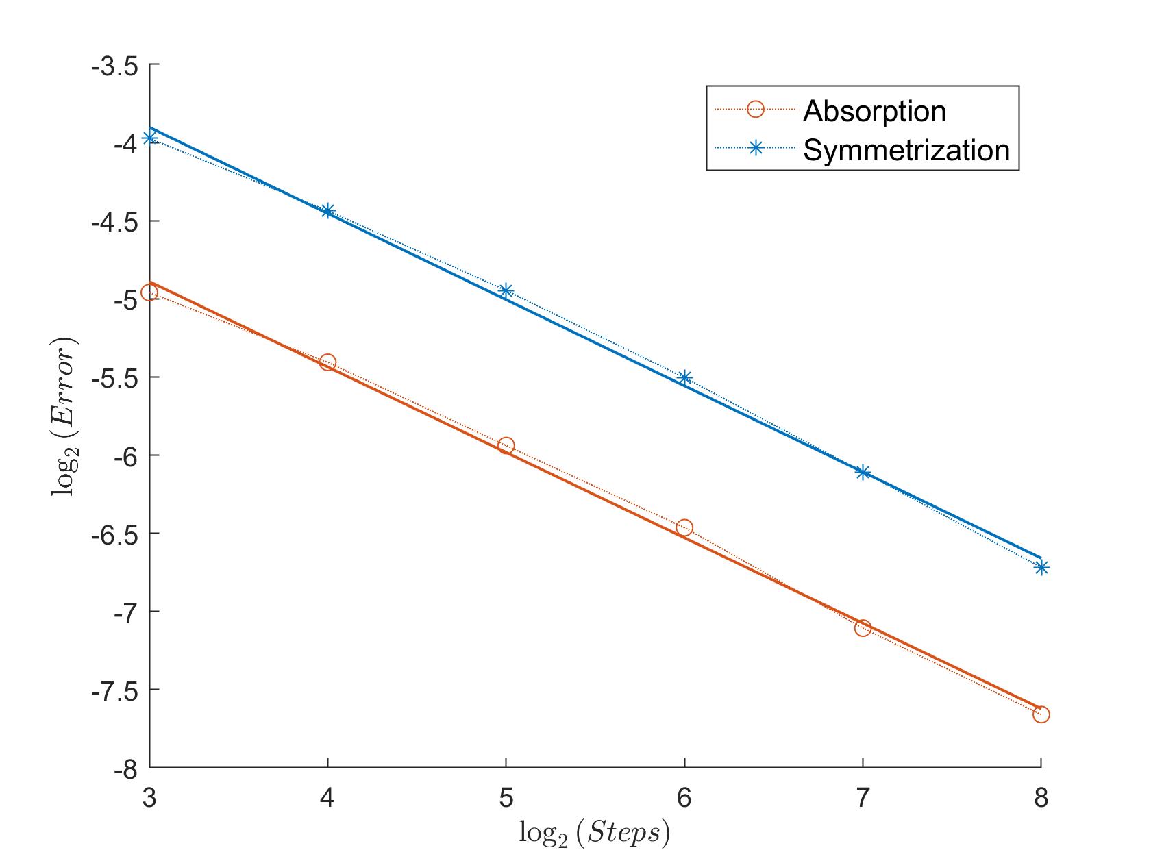
Table 3 shows the estimated convergence rates for Model 3. This model has a Feller index around $0.63$. The simulation results indicate that this is also the convergence rate for SE and AE.

Method Call Put Digital
SE 0.60 0.60 0.55
AE 0.57 0.57 0.55
Table 3: Measured convergence rates Model 3

The error plot of the digital option in Figure 3 again shows no irregularities.

Refer to caption
Figure 3: Digital Model 3

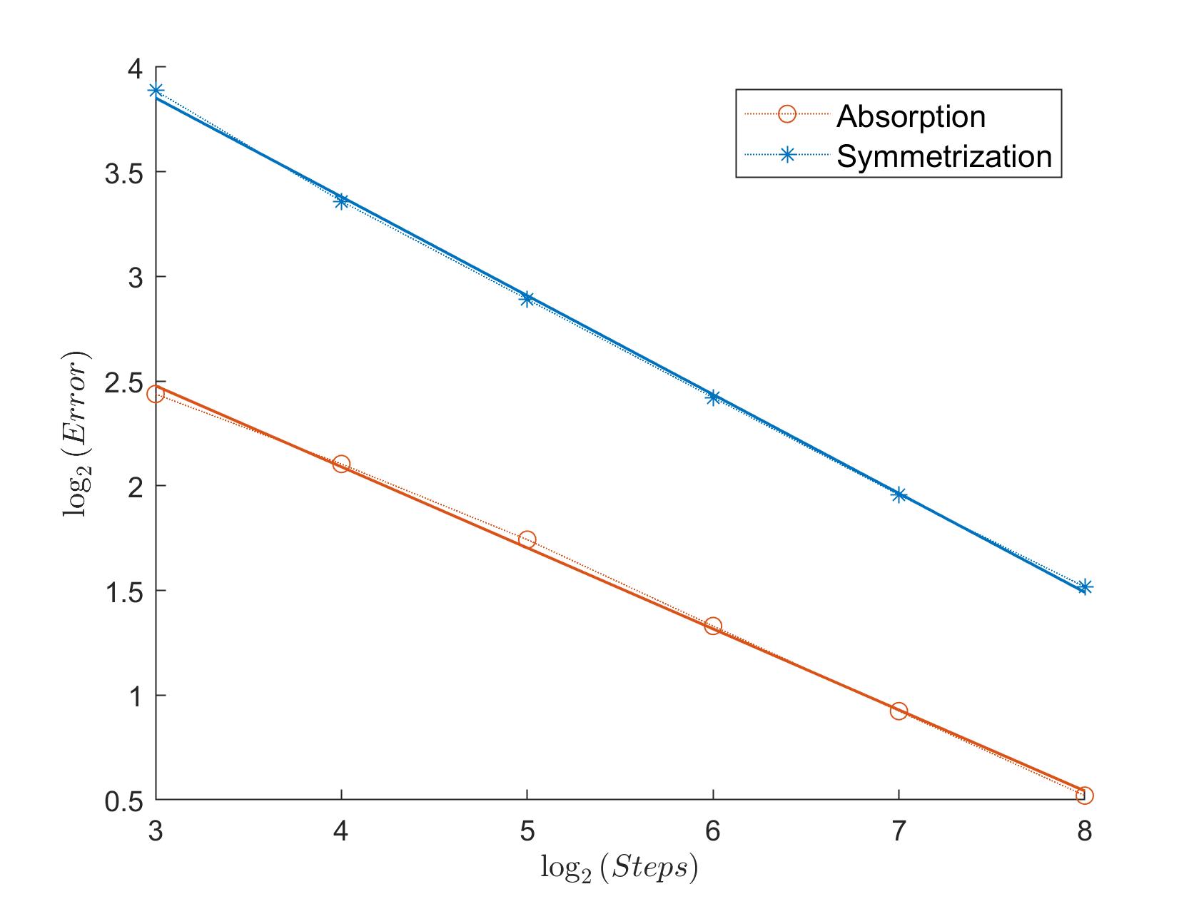
Model 4 has the lowest Feller index which is around $0.36$. Again, Table 4 confirms this number as the numerical convergence rate for SE and AE and the plot in Figure 4 shows a regular behavior.

Method Call Put Digital
SE 0.47 0.47 0.40
AE 0.39 0.39 0.35
Table 4: Measured convergence rates Model 4
Refer to caption
Figure 4: Call Model 4

Summarizing, we can confirm a (minimum) numerical convergence rate of $min\{\nu,1\}$ for the Symmetrized and Absorbed Euler under even milder assumptions on the regularity of the payoff function. We saw even better numerical convergence results for a high Feller index.

Remark 2.1.

Our analysis does not carry over to modified Euler schemes for the CIR process that take negative values, as e.g. the full-truncation Euler [15]. In these schemes the approximation of the CIR component is not bounded from below which prohibits our application of the Kolmogorov PDE and Itลโ€™s lemma. See [36] for a survey on modified Euler schemes.

Remark 2.2.

Bally and Talay analyze in [8] the weak error of the Euler scheme for SDEs with $C_{b}^{\infty}$-coefficients, i.e. coefficients which are infinitely differentiable and whose derivatives of any order are bounded, that satisfy an additional non-degeneracy condition of Hรถrmander type (UH). They establish weak order one for the Euler scheme for test functions $f$ that are only measurable and bounded. However, the log-Heston model does not satisfy the above assumptions and an adaptation of the approach of [8] to the log-Heston model leads to the restrictive assumption $\nu>\frac{9}{2}$ in [4].

The cubature on Wiener space methodology, see [29], is another approach to deal with test functions $f$ of low smoothness. This approach transfers the quadrature of the SDE into the quadrature of a related collection of ordinary differential equations. It allows to handle Lipschitz continuous test functions for SDEs with $C_{b}^{\infty}$-coefficients, which satisfy the (UHG) condition, see [28]. The latter is a relaxation of the (UH) condition.

3 Auxiliary Results

In this section, we will collect and establish several auxiliary results for the weak error analysis.

3.1 Kolmogorov PDE

To obtain the Kolmogorov backward PDE for the Heston Model, we look at the following integral equations:

Vts,vsubscriptsuperscript๐‘‰๐‘ ๐‘ฃ๐‘ก\displaystyle V^{s,v}_{t} =v+โˆซstฮบโ€‹(ฮธโˆ’Vrs,v)โ€‹๐‘‘r+ฯƒโ€‹โˆซstVrs,vโ€‹๐‘‘Wr,absent๐‘ฃsuperscriptsubscript๐‘ ๐‘ก๐œ…๐œƒsubscriptsuperscript๐‘‰๐‘ ๐‘ฃ๐‘Ÿdifferential-d๐‘Ÿ๐œŽsuperscriptsubscript๐‘ ๐‘กsubscriptsuperscript๐‘‰๐‘ ๐‘ฃ๐‘Ÿdifferential-dsubscript๐‘Š๐‘Ÿ\displaystyle=v+\int_{s}^{t}\kappa(\theta-V^{s,v}_{r})dr+\sigma\int_{s}^{t}\sqrt{V^{s,v}_{r}}dW_{r},
Xts,x,vsubscriptsuperscript๐‘‹๐‘ ๐‘ฅ๐‘ฃ๐‘ก\displaystyle{X}^{s,x,v}_{t} =x+ฮผโ€‹(tโˆ’s)โˆ’12โ€‹โˆซstVrs,vโ€‹๐‘‘r+ฯโ€‹โˆซstVrs,vโ€‹๐‘‘Wr+1โˆ’ฯ2โ€‹โˆซstVrs,vโ€‹๐‘‘Br.absent๐‘ฅ๐œ‡๐‘ก๐‘ 12superscriptsubscript๐‘ ๐‘กsubscriptsuperscript๐‘‰๐‘ ๐‘ฃ๐‘Ÿdifferential-d๐‘Ÿ๐œŒsuperscriptsubscript๐‘ ๐‘กsubscriptsuperscript๐‘‰๐‘ ๐‘ฃ๐‘Ÿdifferential-dsubscript๐‘Š๐‘Ÿ1superscript๐œŒ2superscriptsubscript๐‘ ๐‘กsubscriptsuperscript๐‘‰๐‘ ๐‘ฃ๐‘Ÿdifferential-dsubscript๐ต๐‘Ÿ\displaystyle=x+\mu(t-s)-\frac{1}{2}\int_{s}^{t}V^{s,v}_{r}dr+\rho\int_{s}^{t}\sqrt{V^{s,v}_{r}}dW_{r}+\sqrt{1-\rho^{2}}\int_{s}^{t}\sqrt{V^{s,v}_{r}}dB_{r}.

Without loss of generality, we will set $\mu=0$ throughout the remainder of this manuscript. We now define

$\displaystyle u(t,x,v)$ $\displaystyle=\mathbb{E}\left[f\left({X}^{t,x,v}_{T},V^{t,v}_{T}\right)\right],\,t\in[0,T],\,x\in\mathbb{R},\,v\geq 0,$

and let $f\colon\mathbb{R}\times[0,\infty)\rightarrow\mathbb{R}$. The corresponding Kolmogorov backward PDE is then given by

$\displaystyle u_{t}(t,x,v)=$ $\displaystyle\text{ }\frac{v}{2}u_{x}(t,x,v)-\kappa(\theta-v)u_{v}(t,x,v)$ (6)
โˆ’v2โ€‹(uxโ€‹xโ€‹(t,x,v)+2โ€‹ฯโ€‹ฯƒโ€‹uxโ€‹vโ€‹(t,x,v)+ฯƒ2โ€‹uvโ€‹vโ€‹(t,x,v))โ€‹,ย tโˆˆ(0,T),xโˆˆโ„,v>0,formulae-sequence๐‘ฃ2subscript๐‘ข๐‘ฅ๐‘ฅ๐‘ก๐‘ฅ๐‘ฃ2๐œŒ๐œŽsubscript๐‘ข๐‘ฅ๐‘ฃ๐‘ก๐‘ฅ๐‘ฃsuperscript๐œŽ2subscript๐‘ข๐‘ฃ๐‘ฃ๐‘ก๐‘ฅ๐‘ฃ,ย ๐‘ก0๐‘‡formulae-sequence๐‘ฅโ„๐‘ฃ0\displaystyle-\frac{v}{2}\left(u_{xx}(t,x,v)+2\rho\sigma u_{xv}(t,x,v)+\sigma^{2}u_{vv}(t,x,v)\right)\text{, }\quad t\in(0,T),x\in\mathbb{R},v>0,
uโ€‹(T,x,v)=๐‘ข๐‘‡๐‘ฅ๐‘ฃabsent\displaystyle u(T,x,v)= โ€‹fโ€‹(x,v)โ€‹,ย xโˆˆโ„,vโ‰ฅ0.formulae-sequence๐‘“๐‘ฅ๐‘ฃ,ย ๐‘ฅโ„๐‘ฃ0\displaystyle\text{ }f(x,v)\text{, }\quad x\in\mathbb{R},v\geq 0.

In our error analysis we will follow the now classical approach of [38] which exploits the regularity of (6). For the latter we will rely on the recent work of Briani et al. [13]. To state their regularity results, we will need the following notation:


For a multi-index $l=(l_{1},...,l_{d})\in\mathbb{N}^{d}$, we define sโ€‹(l)=โˆ‘j=1dlj๐‘ ๐‘™superscriptsubscript๐‘—1๐‘‘subscript๐‘™๐‘—s(l)=\sum_{j=1}^{d}l_{j} and for $y\in\mathbb{R}^{d}$, we define $\partial^{l}_{y}=\partial^{l_{1}}_{y_{1}}\cdot\cdot\cdot\partial^{l_{d}}_{y_{d}}$. Moreover, we denote by $|y|$ the standard Euclidean norm in $\mathbb{R}^{d}$. Let $\mathcal{D}\subset\mathbb{R}^{d}$ be a domain or a closure of a domain and $q\in\mathbb{N}$. $C^{q}\left(\mathcal{D}\right)$ is the set of all real-valued functions on $\mathcal{D}$ which are $q$-times continuously differentiable. $C^{q}_{pol}\left(\mathcal{D}\right)$ is the set of functions $g\in C^{q}\left(\mathcal{D}\right)$ such that there exist $c,a>0$ for which

|โˆ‚ylgโ€‹(y)|โ‰คcโ€‹(1+|y|a),yโˆˆ๐’Ÿ,sโ€‹(l)โ‰คq.formulae-sequencesubscriptsuperscript๐‘™๐‘ฆ๐‘”๐‘ฆ๐‘1superscript๐‘ฆ๐‘Žformulae-sequence๐‘ฆ๐’Ÿ๐‘ ๐‘™๐‘ž\displaystyle|\partial^{l}_{y}g(y)|\leq c(1+|y|^{a}),\qquad y\in\mathcal{D},\,s(l)\leq q.

We define $C^{q}_{pol,T}\left(\mathcal{D}\right)$ as the set of functions $v\in C^{\lfloor q/2\rfloor,q}_{pol}\left([0,T)\times\mathcal{D}\right)$ such that there exist $c,a>0$ for which

$\displaystyle\sup\limits_{t<T}|\partial^{k}_{t}\partial^{l}_{y}v(t,y)|\leq c(1+|y|^{a}),\qquad y\in\mathcal{D},\,2k+s(l)\leq q.$
Proposition 3.1 (Briani, Caramellino, Terenzi; Proposition 5.3 and Remark 5.4).

Let $q\in\mathbb{N}$ and suppose that $f\in C^{2q}_{pol}(\mathbb{R}\times[0,\infty))$. Then, the solution $u$ of PDE (6) satisfies $u\in C^{q}_{pol,T}(\mathbb{R}\times[0,\infty))$.

Constants whose values depend only on $T$, $x_{0}$, $v_{0}$, $\kappa$, $\theta$, $\sigma$ and $\rho$ will be denoted in the following by $C$, regardless of their value. Other dependencies will be denoted by subscripts, i.e. $C_{f,\beta}$ means that this constant depends additionally on the function $f$ and the parameter $\beta$. Moreover, the value of all these constants can change from line to line.

3.2 Properties of the discretization schemes

We write both volatility schemes as Itล processes for $t\in[t_{k},t_{k+1}]$:

v^tsโ€‹yโ€‹msubscriptsuperscript^๐‘ฃ๐‘ ๐‘ฆ๐‘š๐‘ก\displaystyle\hat{v}^{sym}_{t} =|vnโ€‹(t)sโ€‹yโ€‹m+โˆซฮทโ€‹(t)tฮบโ€‹(ฮธโˆ’vnโ€‹(t)sโ€‹yโ€‹m)โ€‹๐‘‘s+ฯƒโ€‹โˆซฮทโ€‹(t)tvnโ€‹(t)sโ€‹yโ€‹mโ€‹๐‘‘Ws|,absentsuperscriptsubscript๐‘ฃ๐‘›๐‘ก๐‘ ๐‘ฆ๐‘šsuperscriptsubscript๐œ‚๐‘ก๐‘ก๐œ…๐œƒsuperscriptsubscript๐‘ฃ๐‘›๐‘ก๐‘ ๐‘ฆ๐‘šdifferential-d๐‘ ๐œŽsuperscriptsubscript๐œ‚๐‘ก๐‘กsuperscriptsubscript๐‘ฃ๐‘›๐‘ก๐‘ ๐‘ฆ๐‘šdifferential-dsubscript๐‘Š๐‘ \displaystyle=\biggl{|}v_{n(t)}^{sym}+\int_{\eta(t)}^{t}\kappa\left(\theta-v_{n(t)}^{sym}\right)ds+\sigma\int_{\eta(t)}^{t}\sqrt{v_{n(t)}^{sym}}dW_{s}\biggr{|},
v^taโ€‹bโ€‹ssubscriptsuperscript^๐‘ฃ๐‘Ž๐‘๐‘ ๐‘ก\displaystyle\hat{v}^{abs}_{t} =(vnโ€‹(t)aโ€‹bโ€‹s+โˆซฮทโ€‹(t)tฮบโ€‹(ฮธโˆ’vnโ€‹(t)aโ€‹bโ€‹s)โ€‹๐‘‘s+ฯƒโ€‹โˆซฮทโ€‹(t)tvnโ€‹(t)aโ€‹bโ€‹sโ€‹๐‘‘Ws)+.absentsuperscriptsuperscriptsubscript๐‘ฃ๐‘›๐‘ก๐‘Ž๐‘๐‘ superscriptsubscript๐œ‚๐‘ก๐‘ก๐œ…๐œƒsuperscriptsubscript๐‘ฃ๐‘›๐‘ก๐‘Ž๐‘๐‘ differential-d๐‘ ๐œŽsuperscriptsubscript๐œ‚๐‘ก๐‘กsuperscriptsubscript๐‘ฃ๐‘›๐‘ก๐‘Ž๐‘๐‘ differential-dsubscript๐‘Š๐‘ \displaystyle=\left(v_{n(t)}^{abs}+\int_{\eta(t)}^{t}\kappa\left(\theta-v_{n(t)}^{abs}\right)ds+\sigma\int_{\eta(t)}^{t}\sqrt{v_{n(t)}^{abs}}dW_{s}\right)^{+}.

Here we have set $n(t):=\max\{k\in\{0,...,N\}:t_{k}\leq t\}$ and $\eta(t):=t_{n(t)}$. The log-price discretization is the same for both schemes:

$\displaystyle\hat{x}_{t}^{\star}$ =xnโ€‹(t)โ‹†โˆ’12โ€‹โˆซฮทโ€‹(t)tvnโ€‹(t)โ‹†โ€‹๐‘‘s+ฯโ€‹โˆซฮทโ€‹(t)tvnโ€‹(t)โ‹†โ€‹๐‘‘Ws+1โˆ’ฯ2โ€‹โˆซฮทโ€‹(t)tvnโ€‹(t)โ‹†โ€‹๐‘‘Bs,absentsuperscriptsubscript๐‘ฅ๐‘›๐‘กโ‹†12superscriptsubscript๐œ‚๐‘ก๐‘กsuperscriptsubscript๐‘ฃ๐‘›๐‘กโ‹†differential-d๐‘ ๐œŒsuperscriptsubscript๐œ‚๐‘ก๐‘กsuperscriptsubscript๐‘ฃ๐‘›๐‘กโ‹†differential-dsubscript๐‘Š๐‘ 1superscript๐œŒ2superscriptsubscript๐œ‚๐‘ก๐‘กsuperscriptsubscript๐‘ฃ๐‘›๐‘กโ‹†differential-dsubscript๐ต๐‘ \displaystyle=x_{n(t)}^{\star}-\frac{1}{2}\int_{\eta(t)}^{t}v_{n(t)}^{\star}ds+\rho\int_{\eta(t)}^{t}\sqrt{v_{n(t)}^{\star}}dW_{s}+\sqrt{1-\rho^{2}}\int_{\eta(t)}^{t}\sqrt{v_{n(t)}^{\star}}dB_{s},

where $\star\in\{sym,abs\}$. We define

$\displaystyle Z_{t}^{\star}:=v_{n(t)}^{\star}+\kappa\big{(}\theta-v_{n(t)}^{\star}\big{)}(t-\eta(t))+\sigma\sqrt{v_{n(t)}^{\star}}\left(W_{t}-W_{\eta(t)}\right)$ (7)

and use the Tanaka-Meyer formulae for v^tsโ€‹yโ€‹m=|Ztsโ€‹yโ€‹m|subscriptsuperscript^๐‘ฃ๐‘ ๐‘ฆ๐‘š๐‘กsuperscriptsubscript๐‘๐‘ก๐‘ ๐‘ฆ๐‘š\hat{v}^{sym}_{t}=\bigl{|}Z_{t}^{sym}\bigr{|} and for v^taโ€‹bโ€‹s=(Ztaโ€‹bโ€‹s)+subscriptsuperscript^๐‘ฃ๐‘Ž๐‘๐‘ ๐‘กsuperscriptsuperscriptsubscript๐‘๐‘ก๐‘Ž๐‘๐‘ \hat{v}^{abs}_{t}=\left(Z_{t}^{abs}\right)^{+} to obtain

v^tsโ€‹yโ€‹m=vnโ€‹(t)sโ€‹yโ€‹msubscriptsuperscript^๐‘ฃ๐‘ ๐‘ฆ๐‘š๐‘กsuperscriptsubscript๐‘ฃ๐‘›๐‘ก๐‘ ๐‘ฆ๐‘š\displaystyle\hat{v}^{sym}_{t}=v_{n(t)}^{sym} +โˆซฮทโ€‹(t)tsignโก(Zssโ€‹yโ€‹m)โ€‹ฮบโ€‹(ฮธโˆ’vnโ€‹(s)sโ€‹yโ€‹m)โ€‹๐‘‘s+ฯƒโ€‹โˆซฮทโ€‹(t)tsignโก(Zssโ€‹yโ€‹m)โ€‹vnโ€‹(s)sโ€‹yโ€‹mโ€‹๐‘‘Wssuperscriptsubscript๐œ‚๐‘ก๐‘กsignsuperscriptsubscript๐‘๐‘ ๐‘ ๐‘ฆ๐‘š๐œ…๐œƒsuperscriptsubscript๐‘ฃ๐‘›๐‘ ๐‘ ๐‘ฆ๐‘šdifferential-d๐‘ ๐œŽsuperscriptsubscript๐œ‚๐‘ก๐‘กsignsuperscriptsubscript๐‘๐‘ ๐‘ ๐‘ฆ๐‘šsuperscriptsubscript๐‘ฃ๐‘›๐‘ ๐‘ ๐‘ฆ๐‘šdifferential-dsubscript๐‘Š๐‘ \displaystyle+\int_{\eta(t)}^{t}\operatorname{sign}\left(Z_{s}^{sym}\right)\kappa\left(\theta-v_{n(s)}^{sym}\right)ds+\sigma\int_{\eta(t)}^{t}\operatorname{sign}\left(Z_{s}^{sym}\right)\sqrt{v_{n(s)}^{sym}}dW_{s} (8)
+(Lt0โ€‹(Zsโ€‹yโ€‹m)โˆ’Lฮทโ€‹(t)0โ€‹(Zsโ€‹yโ€‹m))superscriptsubscript๐ฟ๐‘ก0superscript๐‘๐‘ ๐‘ฆ๐‘šsuperscriptsubscript๐ฟ๐œ‚๐‘ก0superscript๐‘๐‘ ๐‘ฆ๐‘š\displaystyle+\left(L_{t}^{0}(Z^{sym})-L_{\eta(t)}^{0}(Z^{sym})\right)

and

v^taโ€‹bโ€‹s=ย โ€‹vnโ€‹(t)aโ€‹bโ€‹ssubscriptsuperscript^๐‘ฃ๐‘Ž๐‘๐‘ ๐‘กย superscriptsubscript๐‘ฃ๐‘›๐‘ก๐‘Ž๐‘๐‘ \displaystyle\hat{v}^{abs}_{t}=\text{ }v_{n(t)}^{abs} +โˆซฮทโ€‹(t)t๐Ÿ™{Zsaโ€‹bโ€‹s>0}โ€‹ฮบโ€‹(ฮธโˆ’vnโ€‹(s)aโ€‹bโ€‹s)โ€‹๐‘‘s+ฯƒโ€‹โˆซฮทโ€‹(t)t๐Ÿ™{Zsaโ€‹bโ€‹s>0}โ€‹vnโ€‹(s)aโ€‹bโ€‹sโ€‹๐‘‘Wssuperscriptsubscript๐œ‚๐‘ก๐‘กsubscript1superscriptsubscript๐‘๐‘ ๐‘Ž๐‘๐‘ 0๐œ…๐œƒsuperscriptsubscript๐‘ฃ๐‘›๐‘ ๐‘Ž๐‘๐‘ differential-d๐‘ ๐œŽsuperscriptsubscript๐œ‚๐‘ก๐‘กsubscript1superscriptsubscript๐‘๐‘ ๐‘Ž๐‘๐‘ 0superscriptsubscript๐‘ฃ๐‘›๐‘ ๐‘Ž๐‘๐‘ differential-dsubscript๐‘Š๐‘ \displaystyle+\int_{\eta(t)}^{t}\mathbbm{1}_{\{Z_{s}^{abs}>0\}}\kappa\left(\theta-v_{n(s)}^{abs}\right)ds+\sigma\int_{\eta(t)}^{t}\mathbbm{1}_{\{Z_{s}^{abs}>0\}}\sqrt{v_{n(s)}^{abs}}dW_{s} (9)
+12โ€‹(Lt0โ€‹(Zaโ€‹bโ€‹s)โˆ’Lฮทโ€‹(t)0โ€‹(Zaโ€‹bโ€‹s)).12superscriptsubscript๐ฟ๐‘ก0superscript๐‘๐‘Ž๐‘๐‘ superscriptsubscript๐ฟ๐œ‚๐‘ก0superscript๐‘๐‘Ž๐‘๐‘ \displaystyle+\frac{1}{2}\left(L_{t}^{0}(Z^{abs})-L_{\eta(t)}^{0}(Z^{abs})\right).

Here $L^{0}(Z^{\star})=(L_{t}^{0}(Z^{\star}))_{t\in[0,T]}$ is the local time of $Z^{\star}$ in zero. For almost all $\omega\in\Omega$ the map $[0,T]\ni t\mapsto[L_{t}^{0}(Z^{\star})](\omega)\in\mathbb{R}$ is continuous and non-decreasing with $L_{0}^{0}(Z^{\star})=0$. See e.g.ย Theorem 7.1 in Chapter III of [27].

Moreover, note that

Pโ€‹(Ztsโ€‹yโ€‹m=0|vnโ€‹(t)sโ€‹yโ€‹m=v)=Pโ€‹(Ztaโ€‹bโ€‹s=0|vnโ€‹(t)aโ€‹bโ€‹s=v)=0,vโ‰ฅ0,tโˆˆ[0,T]โˆ–{t0,t1,โ€ฆ,tN},formulae-sequence๐‘ƒsuperscriptsubscript๐‘๐‘ก๐‘ ๐‘ฆ๐‘šconditional0superscriptsubscript๐‘ฃ๐‘›๐‘ก๐‘ ๐‘ฆ๐‘š๐‘ฃ๐‘ƒsuperscriptsubscript๐‘๐‘ก๐‘Ž๐‘๐‘ conditional0superscriptsubscript๐‘ฃ๐‘›๐‘ก๐‘Ž๐‘๐‘ ๐‘ฃ0formulae-sequence๐‘ฃ0๐‘ก0๐‘‡subscript๐‘ก0subscript๐‘ก1โ€ฆsubscript๐‘ก๐‘{P}(Z_{t}^{sym}=0|v_{n(t)}^{sym}=v)={P}(Z_{t}^{abs}=0|v_{n(t)}^{abs}=v)=0,\,\,\qquad v\geq 0,\,t\in[0,T]\setminus\{t_{0},t_{1},\ldots,t_{N}\},

and so $P(Z_{t}^{\star}=0)=0$ for all $t\in[0,T]\setminus\{t_{0},t_{1},\ldots,t_{N}\}$ and $\star\in\{sym,abs\}$.

From [12] we know that the moments of the symmetrized Euler scheme are bounded. This also holds for the Euler scheme with absorption.

Lemma 3.2.

For any $p\geq 1$ we have that

$\displaystyle\mathbb{E}\left[\sup\limits_{t\in[0,T]}\big{|}\hat{v}^{\star}_{t}\big{|}^{p}\right]<\infty$

for $\star\in\{sym,abs\}$.

Proof.

The proof for the symmetrized Euler scheme can be found in [12], the proof for the absorbed Euler scheme can be done analogously. โˆŽ

Furthermore, the discretization of the log-price process also has bounded moments.

Lemma 3.3.

For any $p\geq 1$ we have that

$\displaystyle\mathbb{E}\left[\sup\limits_{t\in[0,T]}\big{|}\hat{x}_{t}^{\star}\big{|}^{p}\right]<\infty$

for $\star\in\{sym,abs\}$.

Proof.

This follows directly from Lemma 3.2 using the Hรถlder and the Burkholder-Davis-Gundy inequalities. โˆŽ

We are now interested in the probability of $Z^{\star}$ becoming less or equal to 00. The next lemma is similar to Lemma 3.7 in [12], and we include its proof for completeness.

Lemma 3.4.

Let $\Delta t<\frac{1}{\kappa}$. We have

$\displaystyle P(Z_{t}^{\star}\leq 0)\leq\mathbb{E}\left[\exp\left(-\frac{{v}_{n(t)}^{\star}(1-\kappa\Delta t)^{2}}{2\sigma^{2}\Delta t}\right)\right],\qquad t\in[0,T]\setminus\{t_{0},t_{1},\ldots,t_{N}\},$

for $\star\in\{sym,abs\}$.

Proof.

Let $t\in[0,T]\setminus\{t_{0},t_{1},\ldots,t_{N}\}$. Since $P(Z_{t}^{\star}=0)=0$ we need to consider only $P(Z_{t}^{\star}<0)$. Throughout this proof, we will drop the $\star$-label to simplify the notation. By the definition of $Z$ in (7), we have

$\displaystyle P(Z_{t}<0|{v}_{n(t)}=v)\leq P\left(W_{t}-W_{\eta(t)}<\frac{-v(1-\kappa(t-\eta(t)))-\kappa\theta(t-\eta(t))}{\sigma\sqrt{v}}\right)$

for $v>0$ and

$\displaystyle P(Z_{t}<0|{v}_{n(t)}=0)=0.$

For a centered Gaussian random variable $G$ with variance $\nu^{2}>0$, it holds that

$\displaystyle P\left(G<\beta\right)\leq\exp\left(-\frac{\beta^{2}}{2\nu^{2}}\right)$

for $\beta<0$. Therefore, we have

$\displaystyle P(Z_{t}\leq 0)$ $\displaystyle\leq\mathbb{E}\left[\exp\left(-\frac{\left({v}_{n(t)}(1-\kappa(t-\eta(t)))+\kappa\theta(t-\eta(t))\right)^{2}}{2\sigma^{2}{v}_{n(t)}(t-\eta(t))}\right)\mathbbm{1}_{\{{v}_{n(t)}>0\}}\right]$
$\displaystyle\leq\mathbb{E}\left[\exp\left(-\frac{\left({v}_{n(t)}(1-\kappa(t-\eta(t)))\right)^{2}}{2\sigma^{2}{v}_{n(t)}(t-\eta(t))}\right)\right]$
$\displaystyle=\mathbb{E}\left[\exp\left(-\frac{{v}_{n(t)}(1-\kappa(t-\eta(t)))^{2}}{2\sigma^{2}(t-\eta(t))}\right)\right].$

Since

$$\frac{(1-\kappa(t-\eta(t)))^{2}}{t-\eta(t)}\geq\frac{(1-\kappa\Delta t)^{2}}{\Delta t},\qquad t\in[0,T]\setminus\{t_{0},t_{1},\ldots,t_{N}\},$$

the assertion follows.

โˆŽ

For the further control of $P(Z_{t}^{\star}\leq 0)$ we will need the following technical result on a sequence that was analyzed by Cozma and Reisinger in [15]. We are now giving a different and simplified bound which is crucial for our error analysis.

Lemma 3.5.

Suppose that $\Delta t<\frac{1}{\kappa}$ and set

$\displaystyle\alpha_{N}=\frac{1-\kappa\Delta t}{2}.$

(i) Consider the sequence $(c_{j})_{0\leq j\leq N}$ with

$\displaystyle c_{0}=\alpha_{N},\qquad c_{1}=\alpha_{N}-\alpha^{2}_{N},\qquad c_{j+1}=c^{2}_{j}+\alpha_{N}-\alpha^{2}_{N},\quad j=1,\ldots,N-1.$

Then, we have

$\displaystyle c_{j}\leq 1-\alpha_{N}-\frac{\varepsilon(1-\varepsilon)}{1+\varepsilon(j-1)},\qquad j=1,\ldots,N,$

for all $\varepsilon\in(0,1/2]$.
(ii) Define the sequence $(a_{j})_{0\leq j\leq N}$ by

$\displaystyle a_{j}=\frac{2(\alpha_{N}-c_{j})}{\sigma^{2}\Delta t},\qquad j=0,\ldots,N.$

Then, we have $a_{j}\geq 0$ for $j=0,\ldots,N$. Moreover, let $\varepsilon\in(0,1/2]$ and

$\displaystyle c=\exp\left(\kappa\left(\nu T+\frac{2v_{0}}{\sigma^{2}}\right)\right)\left(\max\left\{1,\frac{\sigma^{2}\nu}{v_{0}e}\right\}\right)^{\nu}.$ (10)

Then, we have

$\displaystyle\exp\left(-\kappa\theta\sum_{j=0}^{k-1}a_{j+1}\Delta t\right){\exp\left(-v_{0}a_{k+1}\right)}\leq c\left(\frac{\Delta t}{\varepsilon}\right)^{\nu(1-\varepsilon)}$

for all $k=1,\ldots,N$.

Proof.

(i) Since $\Delta t\in(0,\frac{1}{\kappa})$, we know that

$\displaystyle\alpha_{N}=\frac{1-\kappa\Delta t}{2}<\frac{1}{2},\qquad\alpha_{N}>\frac{1-\kappa\frac{1}{\kappa}}{2}=0$

and therefore $\alpha_{N}\in(0,1/2)$. By construction, we then have $c_{j}\geq 0$, $j=0,\ldots,N$. Now let $\varepsilon\in(0,1/2]$. We show that

$\displaystyle c_{j}\leq 1-\alpha_{N}-\frac{1-\varepsilon}{j-1+\varepsilon^{-1}},\qquad j=1,\ldots,N,$

by induction. For $j=1$, we have

$\displaystyle c_{1}=\alpha_{N}-\alpha^{2}_{N}=1-\alpha_{N}-\left(1-\alpha_{N}\right)^{2}\leq 1-\alpha_{N}-\frac{1}{4}\leq 1-\alpha_{N}-\frac{1-\varepsilon}{\varepsilon^{-1}},$

since $1/4\geq(1-\varepsilon)\varepsilon$.

Suppose that the statement holds for a fixed $j\in\{1,...,N\}$. Then, we have

$\displaystyle c_{j+1}=\alpha_{N}-\alpha^{2}_{N}+c^{2}_{j}\leq$ $\displaystyle\,\alpha_{N}-\alpha^{2}_{N}+\left(1-\alpha_{N}-\frac{1-\varepsilon}{j-1+\varepsilon^{-1}}\right)^{2}$
$\displaystyle=$ $\displaystyle\,\alpha_{N}-\alpha^{2}_{N}+1-2\alpha_{N}+\alpha_{N}^{2}-2(1-\alpha_{N})\frac{1-\varepsilon}{j-1+\varepsilon^{-1}}$
$\displaystyle\quad\,\,\,+\frac{(1-\varepsilon)^{2}}{(j-1+\varepsilon^{-1})^{2}}$
$\displaystyle=$ $\displaystyle\,1-\alpha_{N}-2(1-\alpha_{N})\frac{1-\varepsilon}{j-1+\varepsilon^{-1}}+\frac{(1-\varepsilon)^{2}}{(j-1+\varepsilon^{-1})^{2}}.$

Now for

$$c_{j+1}\leq 1-\alpha_{N}-\frac{1-\varepsilon}{j+\varepsilon^{-1}}$$

to be true, it is sufficient that

$\displaystyle\frac{1-\varepsilon}{j-1+\varepsilon^{-1}}-\frac{(1-\varepsilon)^{2}}{(j-1+\varepsilon^{-1})^{2}}\geq\frac{1-\varepsilon}{j+\varepsilon^{-1}}$ (11)

since $2(1-\alpha_{N})\in(1,2)$. Equation (11) can be verified by a simple computation.

(ii) Since $c_{j+1}=c^{2}_{j}+\alpha_{N}-\alpha^{2}_{N}$ and $c_{0}=\alpha_{N}$, $c_{1}=\alpha_{N}-\alpha_{N}^{2}\leq\alpha_{N}$, we can establish by induction that $c_{j}\leq\alpha_{N}$. Since

$$a_{j}=\frac{2(\alpha_{N}-c_{j})}{\sigma^{2}\Delta t}$$

we therefore have $a_{j}\geq 0$ for $j=0,\ldots,N$. It follows that

$\displaystyle-\kappa\theta\sum_{j=0}^{k-1}a_{j+1}\Delta t=\frac{2\kappa\theta}{\sigma^{2}}\sum_{j=0}^{k-1}\left(c_{j+1}-\alpha_{N}\right)$ $\displaystyle\leq\frac{2\kappa\theta}{\sigma^{2}}\sum_{j=0}^{k-1}\left(1-2\alpha_{N}-\frac{1-\varepsilon}{j+\varepsilon^{-1}}\right)$
$\displaystyle\leq\frac{2\kappa\theta}{\sigma^{2}}\int_{0}^{k}\left(1-2\alpha_{N}-\frac{1-\varepsilon}{j+\varepsilon^{-1}}\right)dj$
$\displaystyle=\frac{2\kappa\theta(1-\varepsilon)}{\sigma^{2}}\left(\ln(\varepsilon^{-1})-\ln(k+\varepsilon^{-1})\right)+\frac{2\kappa\theta}{\sigma^{2}}\kappa\Delta tk$
$\displaystyle\leq\nu(1-\varepsilon)\ln\left(\frac{1}{1+\varepsilon k}\right)+\kappa\nu T.$

Using the definition of $a_{k+1}$ and $\alpha_{N}$, as well as the estimate for $c_{k+1}$ from (i) we obtain

$\displaystyle\exp\left(-v_{0}a_{k+1}\right)$ $\displaystyle=\exp\left(\frac{2v_{0}}{\sigma^{2}\Delta t}\left(c_{k+1}-\alpha_{N}\right)\right)$
$\displaystyle\leq\exp\left(\frac{2v_{0}}{\sigma^{2}\Delta t}\left(1-2\alpha_{N}-\frac{\varepsilon(1-\varepsilon)}{1+\varepsilon k}\right)\right)$
$\displaystyle\leq\exp\left(\frac{2v_{0}\kappa}{\sigma^{2}}\right)\exp\left(-\frac{2v_{0}\varepsilon(1-\varepsilon)}{\sigma^{2}}\frac{1}{\Delta t}\frac{1}{1+\varepsilon k}\right)$
$\displaystyle\leq\exp\left(\frac{2v_{0}\kappa}{\sigma^{2}}\right)\exp\left(-\frac{v_{0}\varepsilon}{\sigma^{2}}\frac{1}{\Delta t}\frac{1}{1+\varepsilon k}\right),$

since we have $\varepsilon\in(0,1/2]$. Thus, we obtain

$\displaystyle\exp\left(-\kappa\theta\sum_{j=0}^{k-1}a_{j+1}\Delta t\right)\exp\left(-v_{0}a_{k+1}\right)$
$\displaystyle\qquad\leq\exp\left(\kappa\left(\nu T+\frac{2v_{0}}{\sigma^{2}}\right)\right)\exp\left(-\frac{v_{0}\varepsilon}{\sigma^{2}}\frac{1}{\Delta t}\frac{1}{1+\varepsilon k}\right)\left(\frac{1}{1+\varepsilon k}\right)^{\nu(1-\varepsilon)}$
$\displaystyle\qquad=\exp\left(\kappa\left(\nu T+\frac{2v_{0}}{\sigma^{2}}\right)\right)\exp\left(-\frac{v_{0}\varepsilon}{\sigma^{2}}\frac{1}{\Delta t}\frac{1}{1+\varepsilon k}\right)\left(\frac{v_{0}\varepsilon}{\sigma^{2}}\frac{1}{\Delta t}\frac{1}{1+\varepsilon k}\right)^{\nu(1-\varepsilon)}\left(\frac{\sigma^{2}\Delta t}{v_{0}\varepsilon}\right)^{\nu(1-\varepsilon)}.$

The inequality

$$x^{\alpha}\exp(-x)\leq\alpha^{\alpha}\exp(-\alpha),\qquad\alpha>0,\,x>0,$$

and using again that $\varepsilon\in(0,1/2]$ now yield

$\displaystyle\exp\left(-\kappa\theta\sum_{j=0}^{k-1}a_{j+1}\Delta t\right)\exp\left(-v_{0}a_{k+1}\right)$ $\displaystyle\leq\exp\left(\kappa\left(\nu T+\frac{2v_{0}}{\sigma^{2}}\right)\right)\left(\frac{\nu(1-\varepsilon)}{e}\right)^{\nu(1-\varepsilon)}\left(\frac{\sigma^{2}\Delta t}{v_{0}\varepsilon}\right)^{\nu(1-\varepsilon)}$
$\displaystyle\leq\exp\left(\kappa\left(\nu T+\frac{2v_{0}}{\sigma^{2}}\right)\right)\left(\frac{\sigma^{2}\nu}{v_{0}e}\right)^{\nu(1-\varepsilon)}\left(\frac{\Delta t}{\varepsilon}\right)^{\nu(1-\varepsilon)}$
$\displaystyle\leq\exp\left(\kappa\left(\nu T+\frac{2v_{0}}{\sigma^{2}}\right)\right)\left(\max\left\{1,\frac{\sigma^{2}\nu}{v_{0}e}\right\}\right)^{\nu}\left(\frac{\Delta t}{\varepsilon}\right)^{\nu(1-\varepsilon)},$

which finishes the proof. โˆŽ

The next Lemma gives an upper bound for the expression from Lemma 3.4. It plays the same role as Lemma 3.6 in [12] and in comparison to this Lemma it removes the restriction on $\nu$ and also obtains a better estimate in terms of $\nu$ for $P(Z_{t}^{\star}\leq 0)$.

Proposition 3.6.

For $\Delta t<\frac{1}{\kappa}$ and $\varepsilon\in(0,1/2]$ we have that

$\displaystyle\mathbb{E}\left[\exp\left(-\frac{{v}_{k}^{\star}(1-\kappa\Delta t)^{2}}{2\sigma^{2}\Delta t}\right)\right]\leq c\left(\frac{\Delta t}{\varepsilon}\right)^{\nu(1-\varepsilon)},\qquad k=0,\ldots,N,$ (12)

and

$\displaystyle P(Z_{t}^{\star}\leq 0)\leq c\left(\frac{\Delta t}{\varepsilon}\right)^{\nu(1-\varepsilon)},\qquad t\in[0,T]\setminus\{t_{0},t_{1},\ldots,t_{N}\},$ (13)

for $\star\in\{sym,abs\}$, where $c$ is given by (10).

Proof.

Lemma 3.4 and (12) directly give (13). So it remains to show (12).

The first step of this proof is to describe a sequence $(a_{j})_{0\leq j\leq N}$ whose first element is equal to $\frac{(1-\kappa\Delta t)^{2}}{2\sigma^{2}\Delta t}$ and which has some suitable properties to bound the term on the left side of (12). Suppose that $\Delta t<\frac{1}{\kappa}$. Define the sequence $(a_{j})_{0\leq j\leq N}$ as in the previous Lemma, i.e.

$\displaystyle a_{j}=\frac{2(\alpha_{N}-c_{j})}{\sigma^{2}\Delta t}$

with

$\displaystyle c_{0}=\alpha_{N},\qquad c_{1}=\alpha_{N}-\alpha^{2}_{N},\qquad c_{j+1}=c^{2}_{j}+\alpha_{N}-\alpha^{2}_{N},\quad j=1,\ldots,N-1,$

and $\alpha_{N}=\frac{1-\kappa\Delta t}{2}$. In particular, we have $a_{0}=0,$

$$a_{1}=\frac{2\alpha^{2}_{N}}{\sigma^{2}\Delta t}=\frac{(1-\kappa\Delta t)^{2}}{2\sigma^{2}\Delta t}$$

and

$\displaystyle a_{j+1}=\frac{2(\alpha_{N}-c_{j+1})}{\sigma^{2}\Delta t}=\frac{2(\alpha^{2}_{N}-c^{2}_{j})}{\sigma^{2}\Delta t}=\frac{4\alpha_{N}(\alpha_{N}-c_{j})-2(\alpha_{N}-c_{j})^{2}}{\sigma^{2}\Delta t}=2\alpha_{N}a_{j}-\frac{1}{2}a^{2}_{j}\sigma^{2}\Delta t.$

Next, we take a look at

$\displaystyle\mathbb{E}\left[\exp\left(-{v}_{k}^{\star}a_{i}\right)\right]=\mathbb{E}\left[\mathbb{E}\left[\exp\left(-{v}_{k}^{\star}a_{i}\right)\big{|}\mathcal{F}_{t_{k-1}}\right]\right]$

and bound the conditional expectation using that $a_{i}\geq 0$, $|v|\geq v$ and $v^{+}\geq v$, respectively. We have

$\displaystyle\mathbb{E}\left[\exp\left(-{v}_{k}^{\star}a_{i}\right)\big{|}\mathcal{F}_{t_{k-1}}\right]$
$\displaystyle\quad\leq\mathbb{E}\left[\exp\left(-a_{i}\left(\kappa\theta\Delta t+v_{{k-1}}^{\star}(1-\kappa\Delta t)+\sigma\sqrt{{v}_{{k-1}}^{\star}}\left(W_{t_{k}}-W_{t_{k-1}}\right)\right)\right)\big{|}\mathcal{F}_{t_{k-1}}\right]$
$\displaystyle\quad=\exp\left(-a_{i}\left(\kappa\theta\Delta t+{v}_{{k-1}}^{\star}(1-\kappa\Delta t)\right)\right)\mathbb{E}\left[\exp\left(-a_{i}\sigma\sqrt{{v}_{{k-1}}^{\star}}\left(W_{t_{k}}-W_{t_{k-1}}\right)\right)\big{|}\mathcal{F}_{t_{k-1}}\right]$
$\displaystyle\quad=\exp\left(-a_{i}\left(\kappa\theta\Delta t+{v}_{{k-1}}^{\star}(1-\kappa\Delta t)\right)\right)\exp\left(\frac{1}{2}a^{2}_{i}\sigma^{2}{v}_{{k-1}}^{\star}\Delta t\right).$

Since

$\displaystyle a_{i+1}=a_{i}(1-\kappa\Delta t)-\frac{1}{2}a^{2}_{i}\sigma^{2}\Delta t,$

it follows

$\displaystyle\mathbb{E}\left[\exp\left(-{v}_{k}^{\star}a_{i}\right)\right]\leq\exp\left(-a_{i}\kappa\theta\Delta t\right)\mathbb{E}\left[\exp\left(-{v}_{{k-1}}^{\star}a_{i+1}\right)\right].$

Plugging in $a_{1}$ and applying this upper bound $k$ times, we arrive at

$\displaystyle\mathbb{E}\left[\exp\left(-\frac{{v}_{k}^{\star}(1-\kappa\Delta t)^{2}}{2\sigma^{2}\Delta t}\right)\right]=\mathbb{E}\left[\exp\left(-{v}_{k}^{\star}a_{1}\right)\right]\leq\exp\left(-\kappa\theta\sum_{j=1}^{k}a_{j}\Delta t\right)\exp\left(-v_{0}a_{k+1}\right).$

The assertion now follows from the second part of the previous Lemma. โˆŽ

We also need the following two $L^{p}$-results.

Lemma 3.7.

For all $p\geq 1$ there exists a constant $C_{p}>0$ such that

$\displaystyle\sup\limits_{t\in[0,T]}\mathbb{E}\left[\big{|}\hat{v}_{t}^{\star}-\hat{v}_{\eta(t)}^{\star}\big{|}^{p}\right]\leq C_{p}\left(\Delta t\right)^{\frac{p}{2}}$

holds for $\star\in\{sym,abs\}$.

Proof.

The proof for the Symmetrized Euler can be found in [11]. We prove the statement for the Absorbed Euler by a similar approach and drop the aโ€‹bโ€‹s๐‘Ž๐‘๐‘ abs-label to simplify the notation. We have

$\displaystyle\sup\limits_{t\in[0,T]}\mathbb{E}\left[\left|\hat{v}_{t}-\hat{v}_{\eta(t)}\right|^{p}\right]=\sup\limits_{k=0,...,N-1}\sup\limits_{t\in[t_{k},t_{k+1}]}\mathbb{E}\left[\left|\hat{v}_{t}-\hat{v}_{t_{k}}\right|^{p}\right].$

Since

$\displaystyle\left|\left(v+z\right)^{+}-v\right|\leq|z|$

for $v>0$ and $z\in\mathbb{R}$, we have for $t\in[t_{k},t_{k+1}]$ that

$\displaystyle\left|\hat{v}_{t}-\hat{v}_{t_{k}}\right|^{p}$ $\displaystyle=\left|\left(\hat{v}_{t_{k}}+\kappa\left(\theta-\hat{v}_{t_{k}}\right)(t-t_{k})+\sigma\sqrt{\hat{v}_{t_{k}}}\left(W_{t}-W_{t_{k}}\right)\right)^{+}-\hat{v}_{t_{k}}\right|^{p}$
$\displaystyle\leq\left|\kappa\left(\theta-\hat{v}_{t_{k}}\right)(t-t_{k})+\sigma\sqrt{\hat{v}_{t_{k}}}\left(W_{t}-W_{t_{k}}\right)\right|^{p}$
$\displaystyle\leq 2^{p-1}\left(\Delta t\right)^{p}\left|\kappa\left(\theta-\hat{v}_{t_{k}}\right)\right|^{p}+2^{p-1}\sigma^{p}\hat{v}_{t_{k}}^{p/2}\left|W_{t}-W_{t_{k}}\right|^{p}.$

Using Lemma 3.2 we obtain for all $k=0,\ldots,N-1$ that

$\displaystyle\mathbb{E}\left[\left|\kappa\left(\theta-\hat{v}_{t_{k}}\right)\right|^{p}\right]\leq C_{p}$

and

$\displaystyle\mathbb{E}\left[\hat{v}_{t_{k}}^{p/2}\left|W_{t}-W_{t_{k}}\right|^{p}\right]\leq\left(\mathbb{E}\left[\hat{v}_{t_{k}}^{p}\right]\right)^{\frac{1}{2}}\left(\mathbb{E}\left[\left|W_{t}-W_{t_{k}}\right|^{2p}\right]\right)^{\frac{1}{2}}$ $\displaystyle\leq C_{p}\left(\Delta t\right)^{\frac{p}{2}}.$

Therefore we have

$\displaystyle\sup\limits_{k=0,...,N-1}\sup\limits_{t\in[t_{k},t_{k+1}]}\mathbb{E}\left[\left|\hat{v}_{t}-\hat{v}_{t_{k}}\right|^{p}\right]\leq C_{p}\left(\Delta t\right)^{\frac{p}{2}}$

and the statement follows. โˆŽ

By a similar calculation and with Lemma 3.2, we obtain the following lemma for the discretization of the price process.

Lemma 3.8.

For all $p\geq 1$ there exists a constant $C_{p}>0$ such that

$\displaystyle\sup\limits_{t\in[0,T]}\mathbb{E}\left[\big{|}\hat{x}_{t}^{\star}-\hat{x}^{\star}_{\eta(t)}\big{|}^{p}\right]\leq C_{p}\left(\Delta t\right)^{\frac{p}{2}}$

holds for $\star\in\{sym,abs\}$.

3.3 Properties of the local time

We need an upper bound for the expected local time of $Z^{\star}$ in 00. Our proof follows similar ideas as the proof of Proposition 3.5 in [12], but adds the results from Section 3.2.

Proposition 3.9.

Let $\beta>0$, $\delta>0$, $\varepsilon\in(0,1/2]$, $\Delta t\leq\frac{1}{2\kappa}$ and $\star\in\{sym,abs\}$. Then, there exist constants $C_{\delta}>0$ and $C_{\beta,\delta}>0$ such that

$\displaystyle\mathbb{E}\left[L_{t}^{0}\left(Z^{\star}\right)-L_{\eta(t)}^{0}\left(Z^{\star}\right)\right]\leq C_{\delta}\Delta t\left(\frac{\Delta t}{\varepsilon}\right)^{\nu\frac{1-\varepsilon}{1+\delta}},\qquad t\in[0,T],$

and

$\displaystyle\mathbb{E}\left[\left|L_{t}^{0}\left(Z^{\star}\right)-L_{\eta(t)}^{0}\left(Z^{\star}\right)\right|^{1+\beta}\right]^{\frac{1}{1+\beta}}\leq C_{\beta,\delta}\left(\Delta t\right)^{\frac{1}{(1+\beta)^{2}}}\left(\frac{\Delta t}{\varepsilon}\right)^{\nu\frac{1-\varepsilon}{(1+\delta)(1+\beta)^{2}}}\qquad t\in[0,T].$
Proof.

(i) To simplify the notation, we drop the $\star$-label. By the occupation time formula, see e.g.ย Theorem 7.1 in Chapter III of [27], we have for any $t\in[t_{k},t_{k+1}]$ and for any non-negative Borel-measurable function $\phi:\mathbb{R}\rightarrow\mathbb{R}$ that $P$-a.s

$\displaystyle\int_{\mathbb{R}}\phi(z)\left(L_{t}^{z}\left(Z\right)-L^{z}_{t_{k}}\left(Z\right)\right)dz$ =โˆซtktฯ•โ€‹(Zs)โ€‹dโ€‹โŸจZโŸฉs=ฯƒ2โ€‹โˆซtktฯ•โ€‹(Zs)โ€‹v^tkโ€‹๐‘‘s.absentsuperscriptsubscriptsubscript๐‘ก๐‘˜๐‘กitalic-ฯ•subscript๐‘๐‘ ๐‘‘subscriptdelimited-โŸจโŸฉ๐‘๐‘ superscript๐œŽ2superscriptsubscriptsubscript๐‘ก๐‘˜๐‘กitalic-ฯ•subscript๐‘๐‘ subscript^๐‘ฃsubscript๐‘ก๐‘˜differential-d๐‘ \displaystyle=\int_{t_{k}}^{t}\phi(Z_{s})d\langle Z\rangle_{s}=\sigma^{2}\int_{t_{k}}^{t}\phi(Z_{s})\hat{v}_{t_{k}}ds.

Here $L^{z}(Z)$ is the local time of $Z$ in $z\in\mathbb{R}$. Since

PZs|v^ฮทโ€‹(s)=v=๐’ฉโ€‹(v+ฮบโ€‹(ฮธโˆ’v)โ€‹(sโˆ’ฮทโ€‹(s)),ฯƒ2โ€‹vโ€‹(sโˆ’ฮทโ€‹(s)))superscript๐‘ƒconditionalsubscript๐‘๐‘ subscript^๐‘ฃ๐œ‚๐‘ ๐‘ฃ๐’ฉ๐‘ฃ๐œ…๐œƒ๐‘ฃ๐‘ ๐œ‚๐‘ superscript๐œŽ2๐‘ฃ๐‘ ๐œ‚๐‘ P^{Z_{s}|\hat{v}_{\eta(s)}=v}=\mathcal{N}\left(v+\kappa(\theta-v)(s-\eta(s)),\sigma^{2}v(s-\eta(s))\right)

we have for any $v>0$ that

โˆซโ„ฯ•โ€‹(z)โ€‹๐”ผโ€‹[Ltzโ€‹(Z)โˆ’Ltkzโ€‹(Z)|v^tk=v]โ€‹๐‘‘z=ฯƒ2โ€‹โˆซtktvโ€‹๐”ผโ€‹[ฯ•โ€‹(Zs)|v^tk=v]โ€‹๐‘‘ssubscriptโ„italic-ฯ•๐‘ง๐”ผdelimited-[]superscriptsubscript๐ฟ๐‘ก๐‘ง๐‘conditionalsubscriptsuperscript๐ฟ๐‘งsubscript๐‘ก๐‘˜๐‘subscript^๐‘ฃsubscript๐‘ก๐‘˜๐‘ฃdifferential-d๐‘งsuperscript๐œŽ2superscriptsubscriptsubscript๐‘ก๐‘˜๐‘ก๐‘ฃ๐”ผdelimited-[]conditionalitalic-ฯ•subscript๐‘๐‘ subscript^๐‘ฃsubscript๐‘ก๐‘˜๐‘ฃdifferential-d๐‘ \displaystyle\int_{\mathbb{R}}\phi(z)\mathbb{E}\left[L_{t}^{z}\left(Z\right)-L^{z}_{t_{k}}\left(Z\right)|\hat{v}_{t_{k}}=v\right]dz=\sigma^{2}\int_{t_{k}}^{t}v\mathbb{E}\left[\phi(Z_{s})|\hat{v}_{t_{k}}=v\right]ds
=ฯƒโ€‹โˆซโ„ฯ•โ€‹(z)โ€‹โˆซtktv2โ€‹ฯ€โ€‹(sโˆ’tk)โ€‹expโก(โˆ’(zโˆ’vโˆ’ฮบโ€‹(ฮธโˆ’v)โ€‹(sโˆ’tk))22โ€‹ฯƒ2โ€‹vโ€‹(sโˆ’tk))โ€‹๐‘‘sโ€‹๐‘‘z.๐œŽsubscriptโ„italic-ฯ•๐‘งsuperscriptsubscriptsubscript๐‘ก๐‘˜๐‘ก๐‘ฃ2๐œ‹๐‘ subscript๐‘ก๐‘˜superscript๐‘ง๐‘ฃ๐œ…๐œƒ๐‘ฃ๐‘ subscript๐‘ก๐‘˜22superscript๐œŽ2๐‘ฃ๐‘ subscript๐‘ก๐‘˜differential-d๐‘ differential-d๐‘ง\displaystyle\text{ }=\sigma\int_{\mathbb{R}}\phi(z)\int_{t_{k}}^{t}\frac{\sqrt{v}}{\sqrt{2\pi(s-t_{k})}}\exp\left(-\frac{\left(z-v-\kappa(\theta-v)(s-t_{k})\right)^{2}}{2\sigma^{2}v(s-t_{k})}\right)dsdz.

Since the above equation holds for any non-negative Borel-measurable function $\phi$, we must have that

$\displaystyle\mathbb{E}\left[L_{t}^{z}\left(Z\right)-L^{z}_{t_{k}}\left(Z\right)|\hat{v}_{t_{k}}=v\right]$ =ฯƒโ€‹โˆซtktv2โ€‹ฯ€โ€‹(sโˆ’tk)โ€‹expโก(โˆ’(zโˆ’vโˆ’ฮบโ€‹(ฮธโˆ’v)โ€‹(sโˆ’tk))22โ€‹ฯƒ2โ€‹vโ€‹(sโˆ’tk))โ€‹๐‘‘sabsent๐œŽsuperscriptsubscriptsubscript๐‘ก๐‘˜๐‘ก๐‘ฃ2๐œ‹๐‘ subscript๐‘ก๐‘˜superscript๐‘ง๐‘ฃ๐œ…๐œƒ๐‘ฃ๐‘ subscript๐‘ก๐‘˜22superscript๐œŽ2๐‘ฃ๐‘ subscript๐‘ก๐‘˜differential-d๐‘ \displaystyle=\sigma\int_{t_{k}}^{t}\frac{\sqrt{v}}{\sqrt{2\pi(s-t_{k})}}\exp\left(-\frac{\left(z-v-\kappa(\theta-v)(s-t_{k})\right)^{2}}{2\sigma^{2}v(s-t_{k})}\right)ds

for any $z\in\mathbb{R}$. Setting $z=0$ yields

$\displaystyle\mathbb{E}\left[L_{t}^{0}\left(Z\right)-L_{t_{k}}^{0}\left(Z\right)|\hat{v}_{t_{k}}=v\right]$ =ฯƒโ€‹โˆซtktv2โ€‹ฯ€โ€‹(sโˆ’tk)โ€‹expโก(โˆ’(v+ฮบโ€‹(ฮธโˆ’v)โ€‹(sโˆ’tk))22โ€‹ฯƒ2โ€‹vโ€‹(sโˆ’tk))โ€‹๐‘‘sabsent๐œŽsuperscriptsubscriptsubscript๐‘ก๐‘˜๐‘ก๐‘ฃ2๐œ‹๐‘ subscript๐‘ก๐‘˜superscript๐‘ฃ๐œ…๐œƒ๐‘ฃ๐‘ subscript๐‘ก๐‘˜22superscript๐œŽ2๐‘ฃ๐‘ subscript๐‘ก๐‘˜differential-d๐‘ \displaystyle=\sigma\int_{t_{k}}^{t}\frac{\sqrt{v}}{\sqrt{2\pi(s-t_{k})}}\exp\left(-\frac{\left(v+\kappa(\theta-v)\left(s-t_{k}\right)\right)^{2}}{2\sigma^{2}v\left(s-t_{k}\right)}\right)ds
โ‰คฯƒโ€‹โˆซtktv2โ€‹ฯ€โ€‹(sโˆ’tk)โ€‹expโก(โˆ’vโ€‹(1โˆ’ฮบโ€‹(sโˆ’tk))22โ€‹ฯƒ2โ€‹(sโˆ’tk))โ€‹๐‘‘s.absent๐œŽsuperscriptsubscriptsubscript๐‘ก๐‘˜๐‘ก๐‘ฃ2๐œ‹๐‘ subscript๐‘ก๐‘˜๐‘ฃsuperscript1๐œ…๐‘ subscript๐‘ก๐‘˜22superscript๐œŽ2๐‘ subscript๐‘ก๐‘˜differential-d๐‘ \displaystyle\leq\sigma\int_{t_{k}}^{t}\frac{\sqrt{v}}{\sqrt{2\pi\left(s-t_{k}\right)}}\exp\left(-\frac{v\left(1-\kappa\left(s-t_{k}\right)\right)^{2}}{2\sigma^{2}\left(s-t_{k}\right)}\right)ds.

Since for $\delta>0$ there exist a $c_{\delta}>0$ such that $\sqrt{y}\exp(-y)\leq c_{\delta}\exp\left(-\frac{y}{1+\delta}\right)$ for all $y\geq 0$, we have

vโ€‹(1โˆ’ฮบโ€‹(sโˆ’tk))2โ€‹ฯƒ2โ€‹(sโˆ’tk)โ€‹expโก(โˆ’vโ€‹(1โˆ’ฮบโ€‹(sโˆ’tk))22โ€‹ฯƒ2โ€‹(sโˆ’tk))โ‰คcฮดโ€‹expโก(โˆ’vโ€‹(1โˆ’ฮบโ€‹(sโˆ’tk))22โ€‹ฯƒ2โ€‹(sโˆ’tk)โ€‹(1+ฮด)).๐‘ฃ1๐œ…๐‘ subscript๐‘ก๐‘˜2superscript๐œŽ2๐‘ subscript๐‘ก๐‘˜๐‘ฃsuperscript1๐œ…๐‘ subscript๐‘ก๐‘˜22superscript๐œŽ2๐‘ subscript๐‘ก๐‘˜subscript๐‘๐›ฟ๐‘ฃsuperscript1๐œ…๐‘ subscript๐‘ก๐‘˜22superscript๐œŽ2๐‘ subscript๐‘ก๐‘˜1๐›ฟ\frac{\sqrt{v}(1-\kappa\left(s-t_{k}\right))}{\sqrt{2\sigma^{2}\left(s-t_{k}\right)}}\exp\left(-\frac{{v}\left(1-\kappa\left(s-t_{k}\right)\right)^{2}}{2\sigma^{2}\left(s-t_{k}\right)}\right)\leq c_{\delta}\exp\left(-\frac{{v}\left(1-\kappa\left(s-t_{k}\right)\right)^{2}}{2\sigma^{2}\left(s-t_{k}\right)(1+\delta)}\right).

Moreover, since 1โˆ’ฮบโ€‹(sโˆ’tk)โˆˆ[1/2,1]1๐œ…๐‘ subscript๐‘ก๐‘˜1211-\kappa\left(s-t_{k}\right)\in[1/2,1] we obtain

vsโˆ’tkโ€‹expโก(โˆ’vโ€‹(1โˆ’ฮบโ€‹(sโˆ’tk))22โ€‹ฯƒ2โ€‹(sโˆ’tk))โ‰ค8โ€‹ฯƒโ€‹cฮดโ€‹expโก(โˆ’vโ€‹(1โˆ’ฮบโ€‹(sโˆ’tk))22โ€‹ฯƒ2โ€‹(sโˆ’tk)โ€‹(1+ฮด)).๐‘ฃ๐‘ subscript๐‘ก๐‘˜๐‘ฃsuperscript1๐œ…๐‘ subscript๐‘ก๐‘˜22superscript๐œŽ2๐‘ subscript๐‘ก๐‘˜8๐œŽsubscript๐‘๐›ฟ๐‘ฃsuperscript1๐œ…๐‘ subscript๐‘ก๐‘˜22superscript๐œŽ2๐‘ subscript๐‘ก๐‘˜1๐›ฟ\frac{\sqrt{v}}{\sqrt{s-t_{k}}}\exp\left(-\frac{{v}\left(1-\kappa\left(s-t_{k}\right)\right)^{2}}{2\sigma^{2}\left(s-t_{k}\right)}\right)\leq\sqrt{8}\sigma c_{\delta}\exp\left(-\frac{{v}\left(1-\kappa\left(s-t_{k}\right)\right)^{2}}{2\sigma^{2}\left(s-t_{k}\right)(1+\delta)}\right).

It follows

$\displaystyle\mathbb{E}\left[L_{t}^{0}\left(Z\right)-L_{t_{k}}^{0}\left(Z\right)|\mathcal{F}_{t_{k}}\right]$ โ‰คฯƒโ€‹โˆซtktv^tk2โ€‹ฯ€โ€‹(sโˆ’tk)โ€‹expโก(โˆ’v^tkโ€‹(1โˆ’ฮบโ€‹(sโˆ’tk))22โ€‹ฯƒ2โ€‹(sโˆ’tk))โ€‹๐‘‘sabsent๐œŽsuperscriptsubscriptsubscript๐‘ก๐‘˜๐‘กsubscript^๐‘ฃsubscript๐‘ก๐‘˜2๐œ‹๐‘ subscript๐‘ก๐‘˜subscript^๐‘ฃsubscript๐‘ก๐‘˜superscript1๐œ…๐‘ subscript๐‘ก๐‘˜22superscript๐œŽ2๐‘ subscript๐‘ก๐‘˜differential-d๐‘ \displaystyle\leq\sigma\int_{t_{k}}^{t}\frac{\sqrt{\hat{v}_{t_{k}}}}{\sqrt{2\pi\left(s-t_{k}\right)}}\exp\left(-\frac{\hat{v}_{t_{k}}\left(1-\kappa(s-t_{k})\right)^{2}}{2\sigma^{2}\left(s-t_{k}\right)}\right)ds
โ‰คcฮดโ€‹2โ€‹ฯƒ2ฯ€โ€‹โˆซtktexpโก(โˆ’v^tkโ€‹(1โˆ’ฮบโ€‹(sโˆ’tk))22โ€‹ฯƒ2โ€‹(sโˆ’tk)โ€‹(1+ฮด))โ€‹๐‘‘sabsentsubscript๐‘๐›ฟ2superscript๐œŽ2๐œ‹superscriptsubscriptsubscript๐‘ก๐‘˜๐‘กsubscript^๐‘ฃsubscript๐‘ก๐‘˜superscript1๐œ…๐‘ subscript๐‘ก๐‘˜22superscript๐œŽ2๐‘ subscript๐‘ก๐‘˜1๐›ฟdifferential-d๐‘ \displaystyle\leq c_{\delta}\frac{2\sigma^{2}}{\sqrt{\pi}}\int_{t_{k}}^{t}\exp\left(-\frac{\hat{v}_{t_{k}}\left(1-\kappa(s-t_{k})\right)^{2}}{2\sigma^{2}(s-t_{k})(1+\delta)}\right)ds
โ‰คcฮดโ€‹2โ€‹ฯƒ2ฯ€โ€‹โˆซtktexpโก(โˆ’v^tkโ€‹(1โˆ’ฮบโ€‹ฮ”โ€‹t)22โ€‹ฯƒ2โ€‹ฮ”โ€‹tโ€‹(1+ฮด))โ€‹๐‘‘s.absentsubscript๐‘๐›ฟ2superscript๐œŽ2๐œ‹superscriptsubscriptsubscript๐‘ก๐‘˜๐‘กsubscript^๐‘ฃsubscript๐‘ก๐‘˜superscript1๐œ…ฮ”๐‘ก22superscript๐œŽ2ฮ”๐‘ก1๐›ฟdifferential-d๐‘ \displaystyle\leq c_{\delta}\frac{2\sigma^{2}}{\sqrt{\pi}}\int_{t_{k}}^{t}\exp\left(-\frac{\hat{v}_{t_{k}}\left(1-\kappa\Delta t\right)^{2}}{2\sigma^{2}\Delta t(1+\delta)}\right)ds.

Now, the Lyapunov inequality and Proposition 3.6 yield

$\displaystyle\mathbb{E}\left[L_{t}^{0}\left(Z\right)-L_{t_{k}}^{0}\left(Z\right)\right]$ โ‰คCฮดโ€‹โˆซtkt๐”ผโ€‹[expโก(โˆ’v^tkโ€‹(1โˆ’ฮบโ€‹ฮ”โ€‹t)22โ€‹ฯƒ2โ€‹ฮ”โ€‹tโ€‹(1+ฮด))]โ€‹๐‘‘sabsentsubscript๐ถ๐›ฟsuperscriptsubscriptsubscript๐‘ก๐‘˜๐‘ก๐”ผdelimited-[]subscript^๐‘ฃsubscript๐‘ก๐‘˜superscript1๐œ…ฮ”๐‘ก22superscript๐œŽ2ฮ”๐‘ก1๐›ฟdifferential-d๐‘ \displaystyle\leq C_{\delta}\int_{t_{k}}^{t}\mathbb{E}\left[\exp\left(-\frac{\hat{v}_{t_{k}}\left(1-\kappa\Delta t\right)^{2}}{2\sigma^{2}\Delta t(1+\delta)}\right)\right]ds
$\displaystyle=C_{\delta}\int_{t_{k}}^{t}\mathbb{E}\left[\exp\left(-\frac{\hat{v}_{t_{k}}\left(1-\kappa\Delta t\right)^{2}}{2\sigma^{2}\Delta t}\right)^{\frac{1}{1+\delta}}\right]ds$
โ‰คCฮดโ€‹โˆซtkt(๐”ผโ€‹[expโก(โˆ’v^tkโ€‹(1โˆ’ฮบโ€‹ฮ”โ€‹t)22โ€‹ฯƒ2โ€‹ฮ”โ€‹t)])11+ฮดโ€‹๐‘‘sabsentsubscript๐ถ๐›ฟsuperscriptsubscriptsubscript๐‘ก๐‘˜๐‘กsuperscript๐”ผdelimited-[]subscript^๐‘ฃsubscript๐‘ก๐‘˜superscript1๐œ…ฮ”๐‘ก22superscript๐œŽ2ฮ”๐‘ก11๐›ฟdifferential-d๐‘ \displaystyle\leq C_{\delta}\int_{t_{k}}^{t}\left(\mathbb{E}\left[\exp\left(-\frac{\hat{v}_{t_{k}}\left(1-\kappa\Delta t\right)^{2}}{2\sigma^{2}\Delta t}\right)\right]\right)^{\frac{1}{1+\delta}}ds
$\displaystyle\leq C_{\delta}\Delta t\left(\frac{\Delta t}{\varepsilon}\right)^{\nu\frac{1-\varepsilon}{1+\delta}}.$

(ii) For the second statement note first that

$\displaystyle\mathbb{E}\left[\left|L^{0}_{t}(Z)-L^{0}_{\eta(t)}(Z)\right|^{1+\beta}\right]^{\frac{1}{1+\beta}}$
$\displaystyle\qquad\qquad=\mathbb{E}\left[\left(L^{0}_{t}(Z)-L^{0}_{\eta(t)}(Z)\right)^{\frac{1}{1+\beta}}\left(L^{0}_{t}(Z)-L^{0}_{\eta(t)}(Z)\right)^{\beta+1-\frac{1}{1+\beta}}\right]^{\frac{1}{1+\beta}}$
$\displaystyle\qquad\qquad\leq\left(\mathbb{E}\left[L^{0}_{t}(Z)-L^{0}_{\eta(t)}(Z)\right]\right)^{\frac{1}{(1+\beta)^{2}}}\left(\mathbb{E}\left[\left(L^{0}_{t}(Z)-L^{0}_{\eta(t)}(Z)\right)^{\frac{(\beta+1)^{2}-1}{\beta}}\right]\right)^{\frac{\beta}{(1+\beta)^{2}}}$

by Hรถlderโ€™s inequality. Now, consider first Z=Zsโ€‹yโ€‹m๐‘superscript๐‘๐‘ ๐‘ฆ๐‘šZ=Z^{sym} and note that

$\displaystyle\mathbb{E}\left[\left|L_{t}^{0}\left(Z\right)-L_{\eta(t)}^{0}\left(Z\right)\right|^{p}\right]$
=๐”ผโ€‹[|v^tโˆ’v^ฮทโ€‹(t)โˆ’โˆซฮทโ€‹(t)tsignโก(Zs)โ€‹ฮบโ€‹(ฮธโˆ’v^ฮทโ€‹(s))โ€‹๐‘‘sโˆ’ฯƒโ€‹โˆซฮทโ€‹(t)tsignโก(Zs)โ€‹v^ฮทโ€‹(s)โ€‹๐‘‘Ws|p]absent๐”ผdelimited-[]superscriptsubscript^๐‘ฃ๐‘กsubscript^๐‘ฃ๐œ‚๐‘กsuperscriptsubscript๐œ‚๐‘ก๐‘กsignsubscript๐‘๐‘ ๐œ…๐œƒsubscript^๐‘ฃ๐œ‚๐‘ differential-d๐‘ ๐œŽsuperscriptsubscript๐œ‚๐‘ก๐‘กsignsubscript๐‘๐‘ subscript^๐‘ฃ๐œ‚๐‘ differential-dsubscript๐‘Š๐‘ ๐‘\displaystyle\quad=\mathbb{E}\left[\left|\hat{v}_{t}-\hat{v}_{\eta(t)}-\int_{\eta(t)}^{t}\operatorname{sign}\left(Z_{s}\right)\kappa\left(\theta-\hat{v}_{\eta(s)}\right)ds-\sigma\int_{\eta(t)}^{t}\operatorname{sign}\left(Z_{s}\right)\sqrt{\hat{v}_{\eta(s)}}dW_{s}\right|^{p}\right]
$\displaystyle\quad\leq 3^{p-1}\left(\mathbb{E}\left|\hat{v}_{t}-\hat{v}_{\eta(t)}\right|^{p}+\mathbb{E}\left[\left|\int_{\eta(t)}^{t}\operatorname{sign}\left(Z_{s}\right)\kappa\left(\theta-\hat{v}_{\eta(s)}\right)ds\right|^{p}\right]\right.$
$\displaystyle\qquad\qquad\quad\qquad\qquad\qquad\left.\,+\,\mathbb{E}\left[\left|\sigma\int_{\eta(t)}^{t}\operatorname{sign}\left(Z_{s}\right)\sqrt{\hat{v}_{\eta(s)}}dW_{s}\right|^{p}\right]\right)$

since $|x+y+z|^{p}\leq 3^{p-1}(|x|^{p}+|y|^{p}+|z|^{p})$ for $x,y,z\in\mathbb{R}$, $p\geq 1$. We can conclude from Lemma 3.7, the Hรถlder inequality, the Burkholder-Davis-Gundy inequality and Lemma 3.2 that

$$\sup_{t\in[0,T]}\mathbb{E}\left[\left|L_{t}^{0}\left(Z\right)-L_{\eta(t)}^{0}\left(Z\right)\right|^{p}\right]<\infty.$$

The case Z=Zaโ€‹bโ€‹s๐‘superscript๐‘๐‘Ž๐‘๐‘ Z=Z^{abs} can be done analogously. Applying the estimate from the first part, we obtain

$\displaystyle\mathbb{E}\left[\left|L^{0}_{t}(Z)-L^{0}_{\eta(t)}(Z)\right|^{1+\beta}\right]^{\frac{1}{1+\beta}}$ $\displaystyle\leq C_{\beta}\left(\mathbb{E}\left[L^{0}_{t}(Z)-L^{0}_{\eta(t)}(Z)\right]\right)^{\frac{1}{(1+\beta)^{2}}}$
$\displaystyle\leq C_{\beta,\delta}\left(\Delta t\right)^{\frac{1}{(1+\beta)^{2}}}\left(\frac{\Delta t}{\varepsilon}\right)^{\nu\frac{1-\varepsilon}{(1+\delta)(1+\beta)^{2}}}.$

โˆŽ

4 Proof of Theorem 1.1

Now, we have enough tools to prove our main statement. Since $\mathbb{E}\left[u(T,x_{N}^{\star},v_{N}^{\star})\right]=\mathbb{E}\left[f(x_{N}^{\star},v_{N}^{\star})\right]$ and $u(0,x_{0},v_{0})=\mathbb{E}\left[f(X_{T},V_{T})\right]$ the weak error is a telescoping sum of local errors:

$\displaystyle\left|\mathbb{E}\left[f(x_{N}^{\star},v_{N}^{\star})\right]-\mathbb{E}\left[f(X_{T},V_{T})\right]\right|=\left|\sum_{n=1}^{N}\mathbb{E}\left[u(t_{n},x_{n}^{\star},v_{n}^{\star})-u(t_{n-1},x_{n-1}^{\star},v_{n-1}^{\star})\right]\right|.$

Since v^taโ€‹bโ€‹ssuperscriptsubscript^๐‘ฃ๐‘ก๐‘Ž๐‘๐‘ \hat{v}_{t}^{abs} can be zero with positive probability on a non-empty time interval, technical difficulties with a direct application of the Itล-formula to $u$ at $v=0$, i.e. at the boundary of the state space, arise. Therefore, we will analyze first

$$\left|\sum_{n=1}^{N}\mathbb{E}\left[u(t_{n},x_{n}^{\star},v_{n}^{\star}+\gamma)-u(t_{n-1},x_{n-1}^{\star},v_{n-1}^{\star}+\gamma)\right]\right|$$

with $\gamma>0$ and in a second step exploit that

$\displaystyle|\mathbb{E}\left[f(x_{N},v_{N})-f(X_{T},V_{T})\right]|=\lim_{\gamma\searrow 0}\left|\sum_{n=1}^{N}\mathbb{E}\left[u(t_{n},x_{n}^{\star},v_{n}^{\star}+\gamma)-u(t_{n-1},x_{n-1}^{\star},v_{n-1}^{\star}+\gamma)\right]\right|.$ (14)

This regularization is not required for the symmetrized Euler scheme, but to present both proofs in a concise way, we use it for both schemes. Equation (14) follows e.g. from the smoothness of the Kolmogorov PDE, i.e. Proposition 3.1, and the moment bounds for the discretization schemes, i.e. Lemma 3.2 and 3.3.

Recall that the Kolmogorov PDE is given by

utโ€‹(t,x,v)=subscript๐‘ข๐‘ก๐‘ก๐‘ฅ๐‘ฃabsent\displaystyle u_{t}(t,x,v)= โ€‹โ„’โ€‹(u)โ€‹(t,x,v)โ€‹,ย tโˆˆ(0,T),xโˆˆโ„,v>0,formulae-sequenceโ„’๐‘ข๐‘ก๐‘ฅ๐‘ฃ,ย ๐‘ก0๐‘‡formulae-sequence๐‘ฅโ„๐‘ฃ0\displaystyle\text{ }\mathcal{L}(u)(t,x,v)\text{, }\quad t\in(0,T),x\in\mathbb{R},v>0,
uโ€‹(T,x,v)=๐‘ข๐‘‡๐‘ฅ๐‘ฃabsent\displaystyle u(T,x,v)= โ€‹fโ€‹(x,v)โ€‹,ย xโˆˆโ„,vโ‰ฅ0,formulae-sequence๐‘“๐‘ฅ๐‘ฃ,ย ๐‘ฅโ„๐‘ฃ0\displaystyle\text{ }f(x,v)\text{, }\quad\qquad x\in\mathbb{R},v\geq 0,

with

$$\mathcal{L}(u)(t,x,v)=\frac{v}{2}u_{x}(t,x,v)-\kappa(\theta-v)u_{v}(t,x,v)-\frac{v}{2}\left(u_{xx}(t,x,v)+2\rho\sigma u_{xv}(t,x,v)+\sigma^{2}u_{vv}(t,x,v)\right).$$

For $\gamma\geq 0$, define $u^{\gamma}(t,x,v)=u(t,x,v+\gamma)$. A direct application of Proposition 3.1 gives:

Lemma 4.1.

Let $f\in C^{6}_{pol}(\mathbb{R}\times[0,\infty))$. Then, there exist $C_{f}>0$ and $a>0$ such that

supฮณโˆˆ[0,1]suptโˆˆ[0,T)|โˆ‚xlโˆ‚vmuฮณโ€‹(t,x,v)|โ‰คCfโ€‹(1+|x|a+|1+v|a),ย ย โ€‹xโˆˆโ„,v>0,formulae-sequencesubscriptsupremum๐›พ01subscriptsupremum๐‘ก0๐‘‡subscriptsuperscript๐‘™๐‘ฅsubscriptsuperscript๐‘š๐‘ฃsuperscript๐‘ข๐›พ๐‘ก๐‘ฅ๐‘ฃsubscript๐ถ๐‘“1superscript๐‘ฅ๐‘Žsuperscript1๐‘ฃ๐‘Žformulae-sequenceย ย ๐‘ฅโ„๐‘ฃ0\displaystyle\sup_{\gamma\in[0,1]}\sup\limits_{t\in[0,T)}|\partial^{l}_{x}\partial^{m}_{v}u^{\gamma}(t,x,v)|\leq C_{f}(1+|x|^{a}+|1+v|^{a}),\text{ }\text{ }x\in\mathbb{R},v>0,

if $l+m\leq 3$.

Moreover, note that the function $u^{\gamma}$ satisfies by construction the PDE

$\displaystyle u_{t}^{\gamma}(t,x,v)=$ $\displaystyle\text{ }\mathcal{L}(u^{\gamma})(t,x,v)+\frac{\gamma}{2}\mathcal{R}(u^{\gamma})(t,x,v),$
$\displaystyle u^{\gamma}(T,x,v)=$ $\displaystyle\text{ }f(x,v+\gamma),$

where

$\displaystyle\mathcal{R}(u^{\gamma})(t,x,v)=u_{x}^{\gamma}(t,x,v)+2\kappa u_{v}^{\gamma}(t,x,v)-u_{xx}^{\gamma}(t,x,v)-2\rho\sigma u_{xv}^{\gamma}(t,x,v)-\sigma^{2}u_{vv}^{\gamma}(t,x,v).$

Lemma 4.1 yields

supฮณโˆˆ[0,1]suptโˆˆ[0,T)|โ„›โ€‹(uฮณ)โ€‹(t,x,v)|โ‰คCfโ€‹(1+|x|a+|1+v|a),ย ย โ€‹xโˆˆโ„,v>0,formulae-sequencesubscriptsupremum๐›พ01subscriptsupremum๐‘ก0๐‘‡โ„›superscript๐‘ข๐›พ๐‘ก๐‘ฅ๐‘ฃsubscript๐ถ๐‘“1superscript๐‘ฅ๐‘Žsuperscript1๐‘ฃ๐‘Žformulae-sequenceย ย ๐‘ฅโ„๐‘ฃ0\displaystyle\sup_{\gamma\in[0,1]}\sup\limits_{t\in[0,T)}|\mathcal{R}(u^{\gamma})(t,x,v)|\leq C_{f}(1+|x|^{a}+|1+v|^{a}),\text{ }\text{ }x\in\mathbb{R},v>0, (15)
supฮณโˆˆ[0,1]suptโˆˆ[0,T)|โˆ‚โˆ‚xโ€‹โ„›โ€‹(uฮณ)โ€‹(t,x,v)|โ‰คCfโ€‹(1+|x|a+|1+v|a),ย ย โ€‹xโˆˆโ„,v>0,formulae-sequencesubscriptsupremum๐›พ01subscriptsupremum๐‘ก0๐‘‡๐‘ฅโ„›superscript๐‘ข๐›พ๐‘ก๐‘ฅ๐‘ฃsubscript๐ถ๐‘“1superscript๐‘ฅ๐‘Žsuperscript1๐‘ฃ๐‘Žformulae-sequenceย ย ๐‘ฅโ„๐‘ฃ0\displaystyle\sup_{\gamma\in[0,1]}\sup\limits_{t\in[0,T)}\left|\frac{\partial}{\partial x}\mathcal{R}(u^{\gamma})(t,x,v)\right|\leq C_{f}(1+|x|^{a}+|1+v|^{a}),\text{ }\text{ }x\in\mathbb{R},v>0, (16)
supฮณโˆˆ[0,1]suptโˆˆ[0,T)|โˆ‚โˆ‚vโ€‹โ„›โ€‹(uฮณ)โ€‹(t,x,v)|โ‰คCfโ€‹(1+|x|a+|1+v|a),ย ย โ€‹xโˆˆโ„,v>0.formulae-sequencesubscriptsupremum๐›พ01subscriptsupremum๐‘ก0๐‘‡๐‘ฃโ„›superscript๐‘ข๐›พ๐‘ก๐‘ฅ๐‘ฃsubscript๐ถ๐‘“1superscript๐‘ฅ๐‘Žsuperscript1๐‘ฃ๐‘Žformulae-sequenceย ย ๐‘ฅโ„๐‘ฃ0\displaystyle\sup_{\gamma\in[0,1]}\sup\limits_{t\in[0,T)}\left|\frac{\partial}{\partial v}\mathcal{R}(u^{\gamma})(t,x,v)\right|\leq C_{f}(1+|x|^{a}+|1+v|^{a}),\text{ }\text{ }x\in\mathbb{R},v>0. (17)

We will start with the symmetrized Euler scheme and we will see then that the same procedure can be directly applied to the absorbed Euler scheme.

4.1 The symmetrized Euler scheme

We again drop the sโ€‹yโ€‹m๐‘ ๐‘ฆ๐‘šsym-label to simplify the notation. After the previous preparations, we now apply the Itล formula with $\gamma\in(0,1]$ to the summands of the telescoping sum. Using (5) and (8) we have

$\displaystyle e_{n}^{\gamma}:=$ $\displaystyle\text{ }\mathbb{E}\left[u^{\gamma}(t_{n+1},x_{n+1},v_{n+1})-u^{\gamma}(t_{n},x_{n},v_{n})\right]$
$\displaystyle=$ $\displaystyle\int_{t_{n}}^{t_{n+1}}\mathbb{E}\left[u_{t}^{\gamma}(t,\hat{x}_{t},\hat{v}_{t})-\frac{1}{2}\hat{v}_{\eta(t)}u_{x}^{\gamma}(t,\hat{x}_{t},\hat{v}_{t})+\kappa(\theta-\hat{v}_{\eta(t)})\operatorname{sign}\left(Z_{t}\right)u_{v}^{\gamma}(t,\hat{x}_{t},\hat{v}_{t})\right.$
$\displaystyle\left.\qquad\qquad+\frac{1}{2}\hat{v}_{\eta(t)}u_{xx}^{\gamma}(t,\hat{x}_{t},\hat{v}_{t})+\rho\sigma\hat{v}_{\eta(t)}\operatorname{sign}\left(Z_{t}\right)u_{xv}^{\gamma}(t,\hat{x}_{t},\hat{v}_{t})+\frac{1}{2}\sigma^{2}\hat{v}_{\eta(t)}u_{vv}^{\gamma}(t,\hat{x}_{t},\hat{v}_{t})\right]dt$
$\displaystyle\quad+\mathbb{E}\left[\int_{t_{n}}^{t_{n+1}}u_{v}^{\gamma}(t,\hat{x}_{t},\hat{v}_{t})dL_{t}^{0}(Z)\right]$
$\displaystyle=$ $\displaystyle\int_{t_{n}}^{t_{n+1}}\mathbb{E}\left[u_{t}^{\gamma}(t,\hat{x}_{t},\hat{v}_{t})-\frac{1}{2}\hat{v}_{\eta(t)}u_{x}^{\gamma}(t,\hat{x}_{t},\hat{v}_{t})+\kappa(\theta-\hat{v}_{\eta(t)})u_{v}^{\gamma}(t,\hat{x}_{t},\hat{v}_{t})\right.$
$\displaystyle\left.\qquad\qquad+\frac{1}{2}\hat{v}_{\eta(t)}u_{xx}^{\gamma}(t,\hat{x}_{t},\hat{v}_{t})+\rho\sigma\hat{v}_{\eta(t)}u_{xv}^{\gamma}(t,\hat{x}_{t},\hat{v}_{t})+\frac{1}{2}\sigma^{2}\hat{v}_{\eta(t)}u_{vv}^{\gamma}(t,\hat{x}_{t},\hat{v}_{t})\right]dt$
$\displaystyle\quad-2\int_{t_{n}}^{t_{n+1}}\mathbb{E}\left[\mathbbm{1}_{\{Z_{t}\leq 0\}}\left(\kappa(\theta-\hat{v}_{\eta(t)})u_{v}^{\gamma}(t,\hat{x}_{t},\hat{v}_{t})+\rho\sigma\hat{v}_{\eta(t)}u_{xv}^{\gamma}(t,\hat{x}_{t},\hat{v}_{t})\right)\right]dt$
$\displaystyle\quad+\mathbb{E}\left[\int_{t_{n}}^{t_{n+1}}u_{v}^{\gamma}(t,\hat{x}_{t},\hat{v}_{t})dL_{t}^{0}(Z)\right].$

Note that $t\mapsto L_{t}^{0}(Z)$ is pathwise increasing and that $\int_{t_{n}}^{t_{n+1}}u_{v}^{\gamma}(t,\hat{x}_{t},\hat{v}_{t})dL_{t}^{0}(Z)$ is a pathwise Riemann-Stieltjes integral.

Since

$$u_{t}^{\gamma}(t,x,v)=\text{ }\mathcal{L}(u^{\gamma})(t,x,v)+\frac{\gamma}{2}\mathcal{R}(u^{\gamma})(t,x,v)$$

with

$$\mathcal{L}(u^{\gamma})(t,x,v)=\frac{v}{2}u^{\gamma}_{x}(t,x,v)-\kappa(\theta-v)u^{\gamma}_{v}(t,x,v)-\frac{v}{2}\left(u_{xx}^{\gamma}(t,x,v)+2\rho\sigma u_{xv}^{\gamma}(t,x,v)+\sigma^{2}u_{vv}^{\gamma}(t,x,v)\right)$$

and

$\displaystyle\mathcal{R}(u^{\gamma})(t,x,v)=u_{x}^{\gamma}(t,x,v)+2\kappa u_{v}^{\gamma}(t,x,v)-u_{xx}^{\gamma}(t,x,v)-2\rho\sigma u_{xv}^{\gamma}(t,x,v)-\sigma^{2}u_{vv}^{\gamma}(t,x,v)$

we can write

$\displaystyle e_{n}^{\gamma}=$ $\displaystyle\int_{t_{n}}^{t_{n+1}}\mathbb{E}\left[\frac{\hat{v}_{t}-\hat{v}_{\eta(t)}}{2}\left(u^{\gamma}_{x}(t,\hat{x}_{t},\hat{v}_{t})+2\kappa u^{\gamma}_{v}(t,\hat{x}_{t},\hat{v}_{t})-u_{xx}^{\gamma}(t,\hat{x}_{t},\hat{v}_{t})-2\rho\sigma u_{xv}^{\gamma}(t,\hat{x}_{t},\hat{v}_{t})-\sigma^{2}u^{\gamma}_{vv}(t,\hat{x}_{t},\hat{v}_{t})\right)\right]dt$
$\displaystyle+\frac{\gamma}{2}\int_{t_{n}}^{t_{n+1}}\mathbb{E}\left[\mathcal{R}(u^{\gamma})(t,\hat{x}_{t},\hat{v}_{t})\right]dt$
$\displaystyle-2\int_{t_{n}}^{t_{n+1}}\mathbb{E}\left[\mathbbm{1}_{\{Z_{t}\leq 0\}}\left(\kappa(\theta-\hat{v}_{\eta(t)})u_{v}^{\gamma}(t,\hat{x}_{t},\hat{v}_{t})+\rho\sigma\hat{v}_{\eta(t)}u_{xv}^{\gamma}(t,\hat{x}_{t},\hat{v}_{t})\right)\right]dt$
$\displaystyle+\mathbb{E}\left[\int_{t_{n}}^{t_{n+1}}u_{v}^{\gamma}(t,\hat{x}_{t},\hat{v}_{t})dL_{t}^{0}(Z)\right]$
$\displaystyle=$ $\displaystyle\quad e^{(1,\gamma)}_{n}+e^{(2,\gamma)}_{n}+e^{(3,\gamma)}_{n}+e^{(4,\gamma)}_{n}$

with

$\displaystyle e^{(1,\gamma)}_{n}$ $\displaystyle:=\mathbb{E}\left[\int_{t_{n}}^{t_{n+1}}u^{\gamma}_{v}(t,\hat{x}_{t},\hat{v}_{t})dL_{t}^{0}(Z)\right],$
$\displaystyle e^{(2,\gamma)}_{n}$ $\displaystyle:=-2\int_{t_{n}}^{t_{n+1}}\mathbb{E}\left[\mathbbm{1}_{\{Z_{t}\leq 0\}}\left(\kappa(\theta-\hat{v}_{\eta(t)})u^{\gamma}_{v}(t,\hat{x}_{t},\hat{v}_{t})+\rho\sigma\hat{v}_{\eta(t)}u_{xv}^{\gamma}(t,\hat{x}_{t},\hat{v}_{t})\right)\right]dt,$
$\displaystyle e^{(3,\gamma)}_{n}$ $\displaystyle:=\frac{1}{2}\int_{t_{n}}^{t_{n+1}}\mathbb{E}\left[(\hat{v}_{t}-\hat{v}_{\eta(t)})\mathcal{R}(u^{\gamma})(t,\hat{x}_{t},\hat{v}_{t})\right]dt,$
$\displaystyle e^{(4,\gamma)}_{n}$ $\displaystyle:=\frac{\gamma}{2}\int_{t_{n}}^{t_{n+1}}\mathbb{E}\left[\mathcal{R}(u^{\gamma})(t,\hat{x}_{t},\hat{v}_{t})\right]dt.$

4.1.1 The first term

Recall that $\int_{t_{n}}^{t_{n+1}}u_{v}^{\gamma}(t,\hat{x}_{t},\hat{v}_{t})dL_{t}^{0}(Z)$ is a pathwise Riemann-Stieltjes integral and $L^{0}(Z)$ is pathwise increasing. Therefore we have

$$\left|\int_{t_{n}}^{t_{n+1}}u_{v}^{\gamma}(t,\hat{x}_{t},\hat{v}_{t})dL_{t}^{0}(Z)\right|\leq\sup\limits_{t\in[t_{n},t_{n+1}]}|u_{v}^{\gamma}(t,\hat{x}_{t},\hat{v}_{t})|\left(L^{0}_{t_{n+1}}(Z)-L^{0}_{t_{n}}(Z)\right).$$

With Lemma 4.1 it follows

$\displaystyle\left|\int_{t_{n}}^{t_{n+1}}u_{v}^{\gamma}(t,\hat{x}_{t},\hat{v}_{t})dL_{t}^{0}(Z)\right|$ $\displaystyle\leq C_{f}\sup\limits_{t\in[0,T]}\left(1+|\hat{x}_{t}|^{a}+|1+\hat{v}_{t}|^{a}\right)\left(L^{0}_{t_{n+1}}(Z)-L^{0}_{t_{n}}(Z)\right).$

The Lemmata 3.2 and 3.3 yield the existence of a constant $C_{f,p}>0$ such that

$\displaystyle\left(\mathbb{E}\left|\sup\limits_{t\in[0,T]}\left(1+|\hat{x}_{t}|^{a}+|1+\hat{v}_{t}|^{a}\right)\right|^{p}\right)^{1/p}\leq C_{f,p},$

and Hรถlderโ€™s inequality then gives

$$|e^{(1,\gamma)}_{n}|\leq C_{f,\beta}\left(\mathbb{E}\left|L^{0}_{t_{n+1}}(Z)-L^{0}_{t_{n}}(Z)\right|^{1+\beta}\right)^{\frac{1}{1+\beta}}$$

for $\beta>0$. With Proposition 3.9, we can therefore conclude that

$\displaystyle|e_{n}^{(1,\gamma)}|\leq C_{f,\beta,\delta}\left(\Delta t\right)^{\frac{1}{(1+\beta)^{2}}}\left(\frac{\Delta t}{\varepsilon}\right)^{\nu\frac{1-\varepsilon}{(1+\delta)(1+\beta)^{2}}},$ (18)

uniformly in $\gamma\in(0,1]$.

4.1.2 The second term

Recall that

$\displaystyle e^{(2,\gamma)}_{n}$ $\displaystyle=-2\int_{t_{n}}^{t_{n+1}}\mathbb{E}\left[\mathbbm{1}_{\{Z_{t}\leq 0\}}\left(\kappa(\theta-\hat{v}_{\eta(t)})u_{v}^{\gamma}(t,\hat{x}_{t},\hat{v}_{t})+\rho\sigma\hat{v}_{\eta(t)}u_{xv}^{\gamma}(t,\hat{x}_{t},\hat{v}_{t})\right)\right]dt.$

An application of Hรถlderโ€™s inequality yields

$\displaystyle|e^{(2,\gamma)}_{n}|\leq 2\int_{t_{n}}^{t_{n+1}}\left(P(Z_{t}\leq 0)\right)^{\frac{1}{1+\beta}}\left(\mathbb{E}\left[\left|\kappa(\theta-\hat{v}_{\eta(t)})u_{v}^{\gamma}(t,\hat{x}_{t},\hat{v}_{t})+\rho\sigma\hat{v}_{\eta(t)}u_{xv}^{\gamma}(t,\hat{x}_{t},\hat{v}_{t})\right|^{\frac{1+\beta}{\beta}}\right]\right)^{\frac{\beta}{1+\beta}}dt.$

Lemma 4.1 and the Lemmata 3.2 and 3.3 give that

$\displaystyle 2\left(\mathbb{E}\left[\left|\kappa(\theta-\hat{v}_{\eta(t)})u_{v}^{{\gamma}}(t,\hat{x}_{t},\hat{v}_{t})+\rho\sigma\hat{v}_{\eta(t)}u_{xv}^{{\gamma}}(t,\hat{x}_{t},\hat{v}_{t})\right|^{\frac{1+\beta}{\beta}}\right]\right)^{\frac{\beta}{1+\beta}}\leq C_{f,\beta}$

for $\beta>0$. Since

$$P(Z_{t}\leq 0)\leq c\left(\frac{\Delta t}{\varepsilon}\right)^{\nu(1-\varepsilon)},\qquad t\in(t_{n},t_{n+1}),$$

by Proposition 3.6, we end up with

$\displaystyle|e_{n}^{(2,\gamma)}|\leq C_{f,\beta}\Delta t\left(\frac{\Delta t}{\varepsilon}\right)^{\nu\frac{1-\varepsilon}{1+\beta}},$ (19)

uniformly in $\gamma\in(0,1]$.

4.1.3 The third term

Now, we consider

$$e^{(3,\gamma)}_{n}=\frac{1}{2}\int_{t_{n}}^{t_{n+1}}\mathbb{E}\left[(\hat{v}_{t}-\hat{v}_{\eta(t)})\mathcal{R}(u^{\gamma})(t,\hat{x}_{t},\hat{v}_{t})\right]dt.$$

Due to our assumptions the function $k^{\gamma}:=\mathcal{R}(u^{\gamma})$ belongs to $C^{1}_{pol,T}$. Using the expression for $\hat{v}_{t}$ from Equation (8) we have

$\displaystyle\int_{t_{n}}^{t_{n+1}}\mathbb{E}\left[(\hat{v}_{t}-\hat{v}_{\eta(t)})k^{\gamma}(t,\hat{x}_{t},\hat{v}_{t})\right]dt$
=โˆซtntn+1๐”ผโ€‹[(โˆซฮทโ€‹(t)tsignโก(Zs)โ€‹ฮบโ€‹(ฮธโˆ’v^ฮทโ€‹(s))โ€‹๐‘‘s+ฯƒโ€‹โˆซฮทโ€‹(t)tsignโก(Zs)โ€‹v^ฮทโ€‹(s)โ€‹๐‘‘Ws)โ€‹kฮณโ€‹(t,x^t,v^t)]โ€‹๐‘‘tabsentsuperscriptsubscriptsubscript๐‘ก๐‘›subscript๐‘ก๐‘›1๐”ผdelimited-[]superscriptsubscript๐œ‚๐‘ก๐‘กsignsubscript๐‘๐‘ ๐œ…๐œƒsubscript^๐‘ฃ๐œ‚๐‘ differential-d๐‘ ๐œŽsuperscriptsubscript๐œ‚๐‘ก๐‘กsignsubscript๐‘๐‘ subscript^๐‘ฃ๐œ‚๐‘ differential-dsubscript๐‘Š๐‘ superscript๐‘˜๐›พ๐‘กsubscript^๐‘ฅ๐‘กsubscript^๐‘ฃ๐‘กdifferential-d๐‘ก\displaystyle\quad=\int_{t_{n}}^{t_{n+1}}\mathbb{E}\left[\left(\int_{\eta(t)}^{t}\operatorname{sign}\left(Z_{s}\right)\kappa(\theta-\hat{v}_{\eta(s)})ds+\sigma\int_{\eta(t)}^{t}\operatorname{sign}\left(Z_{s}\right)\sqrt{\hat{v}_{\eta(s)}}dW_{s}\right)k^{\gamma}(t,\hat{x}_{t},\hat{v}_{t})\right]dt
$\displaystyle\qquad+\int_{t_{n}}^{t_{n+1}}\mathbb{E}\left[\left(L_{t}^{0}\left(\hat{v}\right)-L_{\eta(t)}^{0}\left(\hat{v}\right)\right)k^{\gamma}(t,\hat{x}_{t},\hat{v}_{t})\right]dt.$

Looking at the first term, we have using Hรถlderโ€™s inequality, Equation (15) and the Lemmata 3.2, 3.3 that

|๐”ผโ€‹[(โˆซฮทโ€‹(t)tsignโก(Zs)โ€‹ฮบโ€‹(ฮธโˆ’v^ฮทโ€‹(s))โ€‹๐‘‘s)โ€‹kฮณโ€‹(t,x^t,v^t)]|๐”ผdelimited-[]superscriptsubscript๐œ‚๐‘ก๐‘กsignsubscript๐‘๐‘ ๐œ…๐œƒsubscript^๐‘ฃ๐œ‚๐‘ differential-d๐‘ superscript๐‘˜๐›พ๐‘กsubscript^๐‘ฅ๐‘กsubscript^๐‘ฃ๐‘ก\displaystyle\left|\mathbb{E}\left[\left(\int_{\eta(t)}^{t}\operatorname{sign}\left(Z_{s}\right)\kappa(\theta-\hat{v}_{\eta(s)})ds\right)k^{\gamma}(t,\hat{x}_{t},\hat{v}_{t})\right]\right| $\displaystyle\leq C_{f}\Delta t.$ (20)

By an application of the law of total expectation, the Hรถlder and the Minkowski inequalities we have

|๐”ผโ€‹[โˆซฮทโ€‹(t)tsignโก(Zs)โ€‹v^ฮทโ€‹(s)โ€‹๐‘‘Wsโ€‹kฮณโ€‹(t,x^t,v^t)]|๐”ผdelimited-[]superscriptsubscript๐œ‚๐‘ก๐‘กsignsubscript๐‘๐‘ subscript^๐‘ฃ๐œ‚๐‘ differential-dsubscript๐‘Š๐‘ superscript๐‘˜๐›พ๐‘กsubscript^๐‘ฅ๐‘กsubscript^๐‘ฃ๐‘ก\displaystyle\left|\mathbb{E}\left[\int_{\eta(t)}^{t}\operatorname{sign}\left(Z_{s}\right)\sqrt{\hat{v}_{\eta(s)}}dW_{s}k^{\gamma}(t,\hat{x}_{t},\hat{v}_{t})\right]\right|
=|๐”ผโ€‹[โˆซฮทโ€‹(t)tsignโก(Zs)โ€‹v^ฮทโ€‹(s)โ€‹๐‘‘Wsโ€‹(kฮณโ€‹(t,x^t,v^t)โˆ’kฮณโ€‹(t,x^ฮทโ€‹(t),v^ฮทโ€‹(t)))]|absent๐”ผdelimited-[]superscriptsubscript๐œ‚๐‘ก๐‘กsignsubscript๐‘๐‘ subscript^๐‘ฃ๐œ‚๐‘ differential-dsubscript๐‘Š๐‘ superscript๐‘˜๐›พ๐‘กsubscript^๐‘ฅ๐‘กsubscript^๐‘ฃ๐‘กsuperscript๐‘˜๐›พ๐‘กsubscript^๐‘ฅ๐œ‚๐‘กsubscript^๐‘ฃ๐œ‚๐‘ก\displaystyle\quad=\left|\mathbb{E}\left[\int_{\eta(t)}^{t}\operatorname{sign}\left(Z_{s}\right)\sqrt{\hat{v}_{\eta(s)}}dW_{s}\left(k^{\gamma}(t,\hat{x}_{t},\hat{v}_{t})-k^{\gamma}(t,\hat{x}_{\eta(t)},\hat{v}_{\eta(t)})\right)\right]\right|
โ‰ค๐”ผโ€‹[|โˆซฮทโ€‹(t)tsignโก(Zs)โ€‹v^ฮทโ€‹(s)โ€‹๐‘‘Ws|2]12absent๐”ผsuperscriptdelimited-[]superscriptsuperscriptsubscript๐œ‚๐‘ก๐‘กsignsubscript๐‘๐‘ subscript^๐‘ฃ๐œ‚๐‘ differential-dsubscript๐‘Š๐‘ 212\displaystyle\quad\leq\mathbb{E}\left[\left|\int_{\eta(t)}^{t}\operatorname{sign}\left(Z_{s}\right)\sqrt{\hat{v}_{\eta(s)}}dW_{s}\right|^{2}\right]^{\frac{1}{2}}
$\displaystyle\qquad\qquad\times\left[\left(\mathbb{E}\left|(k^{\gamma}(t,\hat{x}_{t},\hat{v}_{t})-k^{\gamma}(t,\hat{x}_{\eta(t)},\hat{v}_{t})\right|^{2}\right)^{1/2}+\left(\mathbb{E}\left|(k^{\gamma}(t,\hat{x}_{\eta(t)},\hat{v}_{t})-k^{\gamma}(t,\hat{x}_{\eta(t)},\hat{v}_{\eta(t)}\right|^{2}\right)^{1/2}\right].$

The mean value theorem now gives

$$k^{\gamma}(t,\hat{x}_{t},\hat{v}_{t})-k^{\gamma}(t,\hat{x}_{\eta(t)},\hat{v}_{t})=\left(\int_{0}^{1}k^{\gamma}_{x}(t,\lambda\hat{x}_{t}+(1-\lambda)\hat{x}_{\eta(t)},\hat{v}_{t})d\lambda\right)(\hat{x}_{t}-\hat{x}_{\eta(t)})$$

and so

$\displaystyle\left(\mathbb{E}\left|k^{\gamma}(t,\hat{x}_{t},\hat{v}_{t})-k^{\gamma}(t,\hat{x}_{\eta(t)},\hat{v}_{t})\right|^{2}\right)^{1/2}$
$\displaystyle\qquad\qquad\quad\leq\left(\int_{0}^{1}\left(\mathbb{E}\left|k^{\gamma}_{x}(t,\lambda\hat{x}_{t}+(1-\lambda)\hat{x}_{\eta(t)},\hat{v}_{t})\right|^{4}\right)^{1/4}d\lambda\right)\left(\mathbb{E}\left|\hat{x}_{t}-\hat{x}_{\eta(t)}\right|^{4}\right)^{1/4}.$

Equation (16) and the Lemmata 3.2, 3.3 imply that

$$\sup_{t\in[0,T]}\int_{0}^{1}\left(\mathbb{E}\left|k^{\gamma}_{x}(t,\lambda\hat{x}_{t}+(1-\lambda)\hat{x}_{\eta(t)},\hat{v}_{t})\right|^{4}\right)^{1/4}d\lambda\leq C_{f}.$$

Thus, we have by Lemma 3.8 that

$$\left(\mathbb{E}\left|k^{\gamma}(t,\hat{x}_{t},\hat{v}_{t})-k^{\gamma}(t,\hat{x}_{\eta(t)},\hat{v}_{t})\right|^{2}\right)^{1/2}\leq C_{f}(\Delta t)^{1/2}.$$

Similarly, we obtain

$$\left(\mathbb{E}\left|k^{\gamma}(t,\hat{x}_{\eta(t)},\hat{v}_{t})-k^{\gamma}(t,\hat{x}_{\eta(t)},\hat{v}_{\eta(t)})\right|^{2}\right)^{1/2}\leq C_{f}(\Delta t)^{1/2}.$$

Since

[๐”ผโ€‹|โˆซฮทโ€‹(t)tsignโก(Zs)โ€‹v^ฮทโ€‹(s)โ€‹๐‘‘Ws|2]12โ‰คCโ€‹(ฮ”โ€‹t)1/2superscriptdelimited-[]๐”ผsuperscriptsuperscriptsubscript๐œ‚๐‘ก๐‘กsignsubscript๐‘๐‘ subscript^๐‘ฃ๐œ‚๐‘ differential-dsubscript๐‘Š๐‘ 212๐ถsuperscriptฮ”๐‘ก12\left[\mathbb{E}\left|\int_{\eta(t)}^{t}\operatorname{sign}\left(Z_{s}\right)\sqrt{\hat{v}_{\eta(s)}}dW_{s}\right|^{2}\right]^{\frac{1}{2}}\leq C(\Delta t)^{1/2}

by Lemma 3.2 and the Itล-isometry, we end up with

|๐”ผโ€‹[(ฯƒโ€‹โˆซฮทโ€‹(t)tsignโก(Zs)โ€‹v^ฮทโ€‹(s)โ€‹๐‘‘Ws)โ€‹kฮณโ€‹(t,x^t,v^t)]|โ‰คCfโ€‹ฮ”โ€‹t.๐”ผdelimited-[]๐œŽsuperscriptsubscript๐œ‚๐‘ก๐‘กsignsubscript๐‘๐‘ subscript^๐‘ฃ๐œ‚๐‘ differential-dsubscript๐‘Š๐‘ superscript๐‘˜๐›พ๐‘กsubscript^๐‘ฅ๐‘กsubscript^๐‘ฃ๐‘กsubscript๐ถ๐‘“ฮ”๐‘ก\displaystyle\left|\mathbb{E}\left[\left(\sigma\int_{\eta(t)}^{t}\operatorname{sign}\left(Z_{s}\right)\sqrt{\hat{v}_{\eta(s)}}dW_{s}\right)k^{\gamma}(t,\hat{x}_{t},\hat{v}_{t})\right]\right|\leq C_{f}\Delta t. (21)

With the Hรถlder inequality for some $\beta>0$, we have

$\displaystyle\left|\int_{t_{n}}^{t_{n+1}}\mathbb{E}\left[\left(L_{t}^{0}(Z)-L_{\eta(t)}^{0}(Z)\right)k^{\gamma}(t,\hat{x}_{t},\hat{v}_{t})\right]dt\right|$
$\displaystyle\qquad\leq\int_{t_{n}}^{t_{n+1}}\left(\mathbb{E}\left|L_{t}^{0}(Z)-L_{\eta(t)}^{0}(Z)\right|^{1+\beta}\right)^{\frac{1}{1+\beta}}\left(\mathbb{E}|k^{\gamma}(t,\hat{x}_{t},\hat{v}_{t})|^{\frac{1+\beta}{\beta}}\right)^{\frac{\beta}{1+\beta}}dt.$

As before, we can show that there exists a constant $C_{f,\beta}>0$, such that

$$\sup_{t\in[0,T]}\left(\mathbb{E}|k^{\gamma}(t,\hat{x}_{t},\hat{v}_{t})|^{\frac{1+\beta}{\beta}}\right)^{\frac{\beta}{1+\beta}}\leq C_{f,\beta}.$$

Since

$$\mathbb{E}\left[\left|L_{t}^{0}(Z)-L_{\eta(t)}^{0}(Z)\right|^{1+\beta}\right]^{\frac{1}{1+\beta}}\leq C_{\beta,\delta}\left(\Delta t\right)^{\frac{1}{(1+\beta)^{2}}}\left(\frac{\Delta t}{\varepsilon}\right)^{\nu\frac{1-\varepsilon}{(1+\delta)(1+\beta)^{2}}},$$

again by Proposition 3.9, we obtain that

$\displaystyle\left|\int_{t_{n}}^{t_{n+1}}\mathbb{E}\left[\left(L_{t}^{0}(Z)-L_{\eta(t)}^{0}(Z)\right)k^{\gamma}(t,\hat{x}_{t},\hat{v}_{t})\right]dt\right|$
$\displaystyle\qquad\leq C_{f,\beta,\delta}\Delta t\left(\Delta t\right)^{\frac{1}{(1+\beta)^{2}}}\left(\frac{\Delta t}{\varepsilon}\right)^{\nu\frac{1-\varepsilon}{(1+\delta)(1+\beta)^{2}}}.$ (22)

Summarizing (20), (21) and (4.1.3) we have shown that

$\displaystyle|e_{n}^{(3,\gamma)}|\leq C_{f,\beta,\delta}\Delta t\left(\Delta t+\left(\Delta t\right)^{\frac{1}{(1+\beta)^{2}}}\left(\frac{\Delta t}{\varepsilon}\right)^{\nu\frac{1-\varepsilon}{(1+\delta)(1+\beta)^{2}}}\right),$ (23)

uniformly in $\gamma\in(0,1]$.

4.1.4 The fourth term

Finally, consider

$$e^{(4,\gamma)}_{n}=\frac{\gamma}{2}\int_{t_{n}}^{t_{n+1}}\mathbb{E}\left[\mathcal{R}(u^{\gamma})(t,\hat{x}_{t},\hat{v}_{t})\right]dt.$$

Since

$$\sup_{t\in[0,T]}\mathbb{E}\left[\mathcal{R}(u^{\gamma})(t,\hat{x}_{t},\hat{v}_{t})\right]\leq C_{f}$$

due to Equation (15) and the Lemmata 3.2, 3.3, we have that

$\displaystyle\frac{1}{\gamma}|e^{(4,\gamma)}_{n}|\leq C_{f}\Delta t,$ (24)

uniformly in $\gamma\in(0,1]$.

4.1.5 The conclusion

Recall that $\Delta t=T/N$. Adding the estimates for term one up to term four we have derived that

$\displaystyle|e_{n}^{\gamma}|$ $\displaystyle\leq C_{f,\beta,\delta}\left(\Delta t\right)^{\frac{1}{(1+\beta)^{2}}}\left(\frac{\Delta t}{\varepsilon}\right)^{\nu\frac{1-\varepsilon}{(1+\delta)(1+\beta)^{2}}}$
$\displaystyle\qquad+C_{f,\beta}\Delta t\left(\frac{\Delta t}{\varepsilon}\right)^{\nu\frac{1-\varepsilon}{1+\beta}}$
$\displaystyle\qquad+C_{f,\beta,\delta}\Delta t\left(\Delta t+\left(\Delta t\right)^{\frac{1}{(1+\beta)^{2}}}\left(\frac{\Delta t}{\varepsilon}\right)^{\nu\frac{1-\varepsilon}{(1+\delta)(1+\beta)^{2}}}\right)$
$\displaystyle\qquad+C_{f}\gamma\Delta t.$

For any given $\epsilon\in(0,1/2)$ we now can find $\varepsilon\in(0,1/2]$, $\beta>0$ and $\delta>0$ such that

$$\frac{1}{(1+\beta)^{2}}+\nu\frac{1-\varepsilon}{(1+\delta)(1+\beta)^{2}}\geq 1+\nu(1-\epsilon)$$

and

$$1+\nu\frac{1-\varepsilon}{1+\beta}\geq 1+\nu(1-\epsilon).$$

Consequently, we obtain

$\displaystyle|e_{n}^{\gamma}|$ $\displaystyle\leq C_{f,\epsilon}\Delta t\left(\Delta t+(\Delta t)^{\nu(1-\epsilon)}\right)+C_{f}\gamma\Delta t$

and

$\displaystyle\sum_{n=0}^{N-1}|e_{n}^{\gamma}|\leq C_{f}\gamma+C_{f,\epsilon}\left(\Delta t+(\Delta t)^{\nu(1-\epsilon)}\right).$

Since

$$|\mathbb{E}\left[f(x_{N},v_{N})-f(X_{T},V_{T})\right]|\leq\limsup_{\gamma\searrow 0}\sum_{n=0}^{N-1}|e_{n}^{\gamma}|$$

we have that

$\displaystyle|\mathbb{E}\left[f(x_{N},v_{N})-f(X_{T},V_{T})\right]|\leq C_{f,\epsilon}\left(\Delta t+(\Delta t)^{\nu(1-\epsilon)}\right),$

which concludes the proof.


4.2 The absorbed Euler scheme

All tools and auxiliary results have been derived simultaneously for the symmetrized and the absorbed Euler scheme. The only difference is that we have

v^taโ€‹bโ€‹s=ย โ€‹vnโ€‹(t)aโ€‹bโ€‹ssubscriptsuperscript^๐‘ฃ๐‘Ž๐‘๐‘ ๐‘กย superscriptsubscript๐‘ฃ๐‘›๐‘ก๐‘Ž๐‘๐‘ \displaystyle\hat{v}^{abs}_{t}=\text{ }v_{n(t)}^{abs} +โˆซฮทโ€‹(t)t๐Ÿ™{Zsaโ€‹bโ€‹s>0}โ€‹ฮบโ€‹(ฮธโˆ’vnโ€‹(s)aโ€‹bโ€‹s)โ€‹๐‘‘s+ฯƒโ€‹โˆซฮทโ€‹(t)t๐Ÿ™{Zsaโ€‹bโ€‹s>0}โ€‹vnโ€‹(s)aโ€‹bโ€‹sโ€‹๐‘‘Wssuperscriptsubscript๐œ‚๐‘ก๐‘กsubscript1superscriptsubscript๐‘๐‘ ๐‘Ž๐‘๐‘ 0๐œ…๐œƒsuperscriptsubscript๐‘ฃ๐‘›๐‘ ๐‘Ž๐‘๐‘ differential-d๐‘ ๐œŽsuperscriptsubscript๐œ‚๐‘ก๐‘กsubscript1superscriptsubscript๐‘๐‘ ๐‘Ž๐‘๐‘ 0superscriptsubscript๐‘ฃ๐‘›๐‘ ๐‘Ž๐‘๐‘ differential-dsubscript๐‘Š๐‘ \displaystyle+\int_{\eta(t)}^{t}\mathbbm{1}_{\{Z_{s}^{abs}>0\}}\kappa\left(\theta-v_{n(s)}^{abs}\right)ds+\sigma\int_{\eta(t)}^{t}\mathbbm{1}_{\{Z_{s}^{abs}>0\}}\sqrt{v_{n(s)}^{abs}}dW_{s}
+12โ€‹(Lt0โ€‹(Zaโ€‹bโ€‹s)โˆ’Lฮทโ€‹(t)0โ€‹(Zaโ€‹bโ€‹s))12superscriptsubscript๐ฟ๐‘ก0superscript๐‘๐‘Ž๐‘๐‘ superscriptsubscript๐ฟ๐œ‚๐‘ก0superscript๐‘๐‘Ž๐‘๐‘ \displaystyle+\frac{1}{2}\left(L_{t}^{0}(Z^{abs})-L_{\eta(t)}^{0}(Z^{abs})\right)

instead of

v^tsโ€‹yโ€‹m=vnโ€‹(t)sโ€‹yโ€‹msubscriptsuperscript^๐‘ฃ๐‘ ๐‘ฆ๐‘š๐‘กsuperscriptsubscript๐‘ฃ๐‘›๐‘ก๐‘ ๐‘ฆ๐‘š\displaystyle\hat{v}^{sym}_{t}=v_{n(t)}^{sym} +โˆซฮทโ€‹(t)tsignโก(Zssโ€‹yโ€‹m)โ€‹ฮบโ€‹(ฮธโˆ’vnโ€‹(s)sโ€‹yโ€‹m)โ€‹๐‘‘s+ฯƒโ€‹โˆซฮทโ€‹(t)tsignโก(Zssโ€‹yโ€‹m)โ€‹vnโ€‹(s)sโ€‹yโ€‹mโ€‹๐‘‘Wssuperscriptsubscript๐œ‚๐‘ก๐‘กsignsuperscriptsubscript๐‘๐‘ ๐‘ ๐‘ฆ๐‘š๐œ…๐œƒsuperscriptsubscript๐‘ฃ๐‘›๐‘ ๐‘ ๐‘ฆ๐‘šdifferential-d๐‘ ๐œŽsuperscriptsubscript๐œ‚๐‘ก๐‘กsignsuperscriptsubscript๐‘๐‘ ๐‘ ๐‘ฆ๐‘šsuperscriptsubscript๐‘ฃ๐‘›๐‘ ๐‘ ๐‘ฆ๐‘šdifferential-dsubscript๐‘Š๐‘ \displaystyle+\int_{\eta(t)}^{t}\operatorname{sign}\left(Z_{s}^{sym}\right)\kappa\left(\theta-v_{n(s)}^{sym}\right)ds+\sigma\int_{\eta(t)}^{t}\operatorname{sign}\left(Z_{s}^{sym}\right)\sqrt{v_{n(s)}^{sym}}dW_{s}
+(Lt0โ€‹(Zsโ€‹yโ€‹m)โˆ’Lฮทโ€‹(t)0โ€‹(Zsโ€‹yโ€‹m)).superscriptsubscript๐ฟ๐‘ก0superscript๐‘๐‘ ๐‘ฆ๐‘šsuperscriptsubscript๐ฟ๐œ‚๐‘ก0superscript๐‘๐‘ ๐‘ฆ๐‘š\displaystyle+\left(L_{t}^{0}(Z^{sym})-L_{\eta(t)}^{0}(Z^{sym})\right).

Besides this difference, we can carry out the proof completely analogous.


Acknowledgments. โ€‰โ€‰ The authors are very thankful to the referees for their insightful comments and remarks, which greatly helped to improve this manuscript. Annalena Mickel has been supported by the DFG Research Training Group 1953 โ€Statistical Modeling of Complex Systemsโ€.

References

  • [1] E.ย Akyildirim, Y.ย Dolinsky, and H.M. Soner. Approximating stochastic volatility by recombinant trees. Ann. Appl. Probab., 24(5):2176 โ€“ 2205, 2014.
  • [2] A.ย Alfonsi. On the discretization schemes for the CIR (and Bessel squared) processes. Monte Carlo Methods Appl., 11(4):355โ€“384, 2005.
  • [3] A.ย Alfonsi. High order discretization schemes for the CIR process: application to affine term structure and Heston models. Math. Comput., 79(269):209โ€“237, 2010.
  • [4] M.ย Altmayer. Quadrature of discontinuous SDE functionals using Malliavin integration by parts. PhD thesis, Mannheim, 2015.
  • [5] M.ย Altmayer and A.ย Neuenkirch. Discretising the Heston model: an analysis of the weak convergence rate. IMA J. Numer. Anal., 37(4):1930โ€“1960, 2017.
  • [6] L.B.G. Andersen. Simple and efficient simulation of the Heston stochastic volatility model. J. Comput. Finance, 11(3):29โ€“50, 2008.
  • [7] L.B.G. Andersen and V.V. Piterbarg. Moment explosions in stochastic volatility models. Finance Stoch., 11(1):29โ€“50, 2007.
  • [8] V.ย Bally and D.ย Talay. The law of the Euler scheme for stochastic differential equations. I: Convergence rate of the distribution function. Probab. Theory Relat. Fields, 104(1):43โ€“60, 1996.
  • [9] Bates, D. Jumps and stochastic volatility: exchange rate processes implicit in Deutsche Mark options. Rev. Financ. Stud.. 9, 69-107 (2015,6)
  • [10] Bayer, C., P. Friz & Gatheral, J. Pricing under rough volatility. Quant. Finance. 16, 887-904 (2016)
  • [11] A.ย Berkaoui, M. Bossy, and A. Diop. Euler scheme for SDEs with non-Lipschitz diffusion coefficient: strong convergence. ESAIM: PS, 12:1โ€“11, 2008.
  • [12] M.ย Bossy and A.ย Diop. An efficient discretisation scheme for one dimensional SDEs with a diffusion coefficient function of the form $|x|^{a}$, $a\in[1/2,1)$. Research Report RR-5396, INRIA, 2007. Version 2.
  • [13] M.ย Briani, L.ย Caramellino, and G.ย Terenzi. Convergence rate of Markov chains and hybrid numerical schemes to jump-diffusions with application to the Bates model. SIAM J. Numer. Anal., 59(1):477โ€“502, 2021.
  • [14] M.ย Broadie and ร–. Kaya. Exact simulation of stochastic volatility and other affine jump diffusion processes. Oper. Res., 54(2):217โ€“231, 2006.
  • [15] A.ย Cozma and C.ย Reisinger. Strong order 1/2 convergence of full truncation Euler approximations to the Cox-Ingersoll-Ross process. IMA J. Numer. Anal., 40(1):1โ€“19, 2018.
  • [16] Z.ย Cui, J.L. Kirkby, and D.ย Nguyen. Efficient simulation of generalized SABR and stochastic local volatility models based on markov chain approximations. European Journal of Operational Research, (to appear), 2020.
  • [17] D.ย Duffie and P.ย Glynn. Efficient Monte Carlo Simulation of Security Prices. Ann. Appl. Probab., 5(4):897 โ€“ 905, 1995.
  • [18] Euch, O. & Rosenbaum, M. The characteristic function of rough Heston models. Math. Financ.. 29, 3-38 (2019)
  • [19] M.B. Giles. Multilevel Monte Carlo path simulation. Oper. Res., 56(3):607โ€“617, 2008.
  • [20] P.ย Glasserman and K.-K. Kim. Gamma expansion of the Heston stochastic volatility model. Finance Stoch., 15(2):267โ€“296, 2011.
  • [21] Grzelak, L., Witteveen, J., Suรกrez-Taboada, M. & Oosterlee, C. The stochastic collocation Monte Carlo sampler: highly efficient sampling from โ€˜expensiveโ€™ distributions. Quant. Finance. 19, 339-356 (2019)
  • [22] M.ย Hefter and A.ย Herzwurm. Strong convergence rates for Cox-Ingersoll-Ross processes โ€“ full parameter range. J. Math. Anal. Appl., 459(2):1079โ€“1101, 2018.
  • [23] M.ย Hefter and A.ย Jentzen. On arbitrarily slow convergence rates for strong numerical approximations of Cox-Ingersoll-Ross processes and squared Bessel processes. Finance Stoch., 23(1):139โ€“172, 2019.
  • [24] S.L. Heston. A closed-form solution for options with stochastic volatility with applications to bond and currency options. Rev. Financial Studies, 6(2):327โ€“343, 1993.
  • [25] D.J. Higham and X.ย Mao. Convergence of Monte Carlo simulations involving the mean-reverting square root process. J. Comp. Fin., 8:35โ€“61, 2005.
  • [26] C.ย Kahl and P.ย Jรคckel. Fast strong approximation Monte-Carlo schemes for stochastic volatility models. Quant. Finance, 6(6):513โ€“536, 2006.
  • [27] I.ย Karatzas and S.E. Shreve. Brownian motion and stochastic calculus. New York, Springer-Verlag, 2nd edition, 1991.
  • [28] Kusuoka, S. Approximation of expectation of diffusion process and mathematical finance. Taniguchi Conference On Mathematics Nara โ€™98. Papers From The Conference, Nara, Japan, December 15โ€“20, 1998. pp. 147-165 (2001)
  • [29] Lyons, T. & Victoir, N. Cubature on Wiener space. Proc. R. Soc. Lond., Ser. A, Math. Phys. Eng. Sci.. 460, 169-198 (2004)
  • [30] Malham, S., Shen, J. & Wiese, A. Series Expansions and Direct Inversion for the Heston Model. SIAM J. Financial Math.. 12, 487-549 (2021)
  • [31] S.J. Malham and A.ย Wiese. Chi-square simulation of the CIR process and the Heston model. Int. J. Theor. Appl. Finance, 16(3), 2013.
  • [32] A.ย Mickel and A.ย Neuenkirch. The weak convergence rate of two semi-exact discretization schemes for the Heston model. Risks, 9(1), 2021.
  • [33] Mickel, A. & Neuenkirch, A. Sharp $L^{1}$-Approximation of the log-Heston SDE by Euler-type methods. ArXiv:2206.03229. (2022)
  • [34] Ninomiya, M. & Ninomiya, S. A new higher-order weak approximation scheme for stochastic differential equations and the Runge-Kutta method. Finance Stoch.. 13, 415-443 (2009)
  • [35] S.ย Ninomiya and N.ย Victoir. Weak approximation of stochastic differential equations and application to derivative pricing. Appl. Math. Finance, 15(2):107โ€“121, 2008.
  • [36] R. Lord, R. Koekkoek, and D.J.C. van Dijk. A comparison of biased simulation schemes for stochastic volatility models. Quant. Finance, 10(2):177โ€“194, 2009.
  • [37] R.D. Smith. An almost exact simulation method for the Heston model. J. Comput. Finance, 11(1):115โ€“125, 2007.
  • [38] D.ย Talay and L.ย Tubaro. Expansion of the global error for numerical schemes solving stochastic differential equations. Stochastic Anal. Appl., 8(4):483โ€“509, 1990.
  • [39] C.ย Zheng. Weak Convergence Rate of a Time-Discrete Scheme for the Heston Stochastic Volatility. SIAM J. Numer. Anal., 55(3):1243โ€“1263, 2017.