HUPD-2104 Electron EDM arising from modulus $\tau$
in the supersymmetric modular invariant flavor models

1 Introduction

The non-Abelian discrete groups have been discussed to challenge the flavor problem of quarks and leptons in the standard model (SM) [1, 2, 3, 4, 5, 6, 7, 8, 9, 10]. Indeed, supersymmetric (SUSY) modular invariant theories give us an attractive framework to address the flavor symmetry of quarks and leptons with non-Abelian discrete groups [11]. In this approach, the quark and lepton mass matrices are written in terms of modular forms which are holomorphic functions of the modulus $\tau$. The arbitrary symmetry breaking sector of the conventional models based on flavor symmetries is replaced by the moduli space, and then Yukawa couplings are given by modular forms.

The well-known finite groups $\rm S_{3}$, $\rm A_{4}$, $\rm S_{4}$, and $\rm A_{5}$ are isomorphic to the finite modular groups $\Gamma_{N}$ for $N=2,3,4,5$, respectively[12]. The lepton mass matrices have been given successfully in terms of $\rm A_{4}$ modular forms [11]. Modular invariant flavor models have been also proposed on the $\Gamma_{2}\simeq\rm S_{3}$ [13], $\Gamma_{4}\simeq\rm S_{4}$ [14] and $\Gamma_{5}\simeq\rm A_{5}$ [15]. Based on these modular forms, flavor mixing of quarks and leptons have been discussed intensively in these years. Phenomenological studies of the lepton flavors have been done based on $\rm A_{4}$ [16, 17, 18], $\rm S_{4}$ [19, 20, 21] and $\rm A_{5}$ [22]. A clear prediction of the neutrino mixing angles and the Dirac CP phase was given in the simple lepton mass matrices with the $\rm A_{4}$ modular symmetry [17]. The Double Covering groups $\rm T^{\prime}$ [23, 24] and $\rm S_{4}^{\prime}$ [25, 26] were also realized in the modular symmetry. Furthermore, phenomenological studies have been developed in many works [27, 29, 28, 30, 31, 32, 33, 34, 35, 36, 37, 38, 39, 40, 41, 42, 43, 44, 45, 46, 47, 48, 49, 50, 51, 52, 53, 54, 55, 56, 57, 58, 59, 60, 61, 62, 63, 64, 65, 66, 67, 68, 69, 70, 71, 72, 75, 73, 74, 76, 77] while theoretical investigations have been also proceeded [78, 79, 80, 82, 81, 85, 86, 84, 83, 87, 88, 89, 90, 91, 92, 93, 94, 95, 96, 97].

The supersymmetric modular invariant theory of flavors addresses not only the flavor structure of quarks and leptons, but also the flavor structure of their superpartners and leads to specific patterns in soft SUSY breaking terms [73, 74]. Soft SUSY breaking terms were studied in several models with non-Abelian flavor symmetries [98, 99, 100, 101, 102]. Such physics can be observed indirectly in the low energy experiments like lepton flavor violating (LFV) processes [74].

The vacuum expectation value (VEV) of the modulus $\tau$ plays an important role in modular flavor symmetry, in particular realization of quark and lepton masses and their mixing angles. The modulus VEV is fixed as the potential minimum of the modulus potential, so called the modulus stabilization in modular flavor models [80, 89, 88, 86]. At such a minimum, the F-term of the modulus $F^{\tau}$ may be non-vanishing, and leads to SUSY breaking, that is the moduli-mediated SUSY breaking [103, 104, 105, 106]. This specific pattern of soft SUSY breaking terms has been discussed in the LFV [74].

On the other hand, the modular invariance has been also studied in the framework of the generalized CP symmetry [107], which is the non-trivial CP transformation in the non-Abelian discrete flavor symmetry [108, 109, 110, 111, 112, 113]. A viable CP invariant lepton model was proposed in the modular $\rm A_{4}$ symmetry [68], in which the CP symmetry is broken by fixing $\tau$, that is, the breaking of the modular symmetry (see also [69]). The phenomenological implication of those models were studied by focusing the Pontecorvo-Maki-Nakagawa-Sakata (PMNS) mixing angles [114, 115] and the CP violating Dirac phase of leptons. In this framework, a fixed $\tau$ also causes the CP violation in the soft SUSY breaking terms. The electric dipole moments (EDMs) of charged leptons arise from the CP non-conserved soft SUSY breaking terms. The current experimental upper bound of the electron EDM, $|d_{e}/e|\leq 1.1\times 10^{-29}$ cm at 90% confidence level has been reported by the ACME Collaboration [116], and the future sensitivity is expected to reach up to $|d_{e}/e|\simeq 10^{-30}$ cm [117, 118]. This future sensitivity put forward the theoretical studies of some models [119, 120].

In our work, we discuss the electron EDM in the framework of the supersymmetric modular invariant theory of flavors. We take the level 3 finite modular groups, $\Gamma_{3}$ for the flavor symmetry since the property of $\rm A_{4}$ flavor symmetry has been well known [121, 122, 123, 124, 125, 126, 127]. Indeed, viable CP invariant lepton models have been investigated linking to the leptogenesis recently [128]. In this flavor symmetry, we study the electron EDM by fixing $\tau$ in the soft SUSY breaking term while the observed lepton masses and PMNS mixing angles are completely reproduced. The SUSY mass scale is also significantly constrained [74] by inputting the observed upper bound of LFV, that is the $\mu\rightarrow e\gamma$ decay [129]. In order to see the effect of CP phase in the modulus $\tau$, we examine the correlation between the electron EDM and the decay rate of the $\mu\rightarrow e\gamma$ decay. The correlation is clearly seen by putting the SUSY mass parameters. That is contrast to the case of the conventional non-abelian discrete flavor symmetric model [130, 131, 102]. Indeed, our mass insertion parameters are obtained without uncertainty once the lepton mass matrices and the SUSY mass scale are fixed.

The paper is organized as follows. In section 2, we give a brief review on the CP transformation in the modular symmetry. In section 3, we present the soft SUSY breaking terms in the modular flavor models. In section 4, we present the CP invariant lepton mass matrix in the $\rm A_{4}$ modular symmetry. In section 5, we present formulae for the electron EDM and the branching ratio of the $\mu\rightarrow e\gamma$ decay in terms of the soft SUSY breaking masses. In section 6, we present the numerical result of the electron EDM as well as the branching ratio of the $\mu\rightarrow e\gamma$ decay. Section 7 is devoted to the summary. In Appendices A and B, we give the tensor product of the $\rm A_{4}$ group and the modular forms, respectively. In Appendices C and D, we present the relevant renormalization group equations (RGEs) and loop functions, respectively. In Appendix E, we show the charged lepton mass matrix with only weight 2 modular forms and corresponding slepton mass matrix.

2 CP transformation in modular symmetry

2.1 Generalized CP symmetry

The CP transformation is non-trivial if the non-Abelian discrete flavor symmetry $G$ is set in the Yukawa sector of a Lagrangian [113, 132]. Let us consider the chiral superfields. The CP is a discrete symmetry which involves both Hermitian conjugation of a chiral superfield $\psi(x)$ and inversion of spatial coordinates,

$$\psi(x)\rightarrow{\bf X}_{\bf r}\overline{\psi}(x_{P})\ ,$$ (1)

where $x_{P}=(t,-{\bf x})$ and ${\bf X_{r}}$ is a unitary transformation of $\psi(x)$ in the irreducible representation $\bf r$ of the discrete flavor symmetry $G$. This transformation is called a generalized CP transformation. If ${\bf X_{r}}$ is the unit matrix, the CP transformation is the trivial one. This is the case for the continuous flavor symmetry [132]. However, in the framework of the non-Abelian discrete family symmetry, non-trivial choices of ${\bf X_{r}}$ are possible. The unbroken CP transformations of ${\bf X_{r}}$ form the group $H_{CP}$. Then, ${\bf X_{r}}$ must be consistent with the flavor symmetry transformation,

$$\psi(x)\rightarrow{\rho}_{\bf r}(g)\psi(x)\ ,\quad g\in G\ ,$$ (2)

where ${\rho}_{\bf{r}}(g)$ is the representation matrix for $g$ in the irreducible representation $\bf{r}$.

The condition, which has to be respected for consistent implementation of a generalized CP symmetry along with a flavor symmetry, is given as follows [133, 135, 134]:

$${\bf X}_{\bf r}\rho_{\bf r}^{*}(g){\bf X}^{-1}_{\bf r}={\rho}_{\bf r}(g^{\prime})\ ,\qquad g,\,g^{\prime}\in G\ .$$ (3)

This is called the consistency condition for ${\bf X}_{\bf r}$.

2.2 Modular symmetry

The modular group $\bar{\Gamma}$ is the group of linear fractional transformations $\gamma$ acting on the modulus $\tau$, belonging to the upper-half complex plane as:

$$\tau\longrightarrow\gamma\tau=\frac{a\tau+b}{c\tau+d}\ ,~{}~{}{\rm where}~{}~{}a,b,c,d\in\mathbb{Z}~{}~{}{\rm and}~{}~{}ad-bc=1,~{}~{}{\rm Im}[\tau]>0~{},$$ (4)

which is isomorphic to $PSL(2,\mathbb{Z})=SL(2,\mathbb{Z})/\{\rm I,-I\}$ transformation. This modular transformation is generated by $S$ and $T$,

$$S:\tau\longrightarrow-\frac{1}{\tau}\ ,\qquad\qquad T:\tau\longrightarrow\tau+1\ ,$$ (5)

which satisfy the following algebraic relations,

$$S^{2}=\mathbb{1}\ ,\qquad(ST)^{3}=\mathbb{1}\ .$$ (6)

We introduce the series of groups $\Gamma(N)$, called principal congruence subgroups, where $N$ is the level $1,2,3,\dots$. These groups are defined by

$$\begin{aligned} \Gamma(N)=\left\{\begin{pmatrix}a&b\\ c&d\end{pmatrix}\in SL(2,\mathbb{Z})~{},~{}~{}\begin{pmatrix}a&b\\ c&d\end{pmatrix}=\begin{pmatrix}1&0\\ 0&1\end{pmatrix}~{}~{}({\rm mod}N)\right\}\end{aligned}.$$ (7)

For $N=2$, we define $\bar{\Gamma}(2)\equiv\Gamma(2)/\{\rm I,-I\}$. Since the element $\rm-I$ does not belong to $\Gamma(N)$ for $N>2$, we have $\bar{\Gamma}(N)=\Gamma(N)$. The quotient groups defined as $\Gamma_{N}\equiv\bar{\Gamma}/\bar{\Gamma}(N)$ are finite modular groups. In these finite groups $\Gamma_{N}$, $T^{N}=\mathbb{1}$ is imposed. The groups $\Gamma_{N}$ with $N=2,3,4,5$ are isomorphic to $\rm S_{3}$, $\rm A_{4}$, $\rm S_{4}$ and $\rm A_{5}$, respectively [12].

Modular forms $f_{i}(\tau)$ of weight $k$ are the holomorphic functions of $\tau$ and transform as

$$f_{i}(\tau)\longrightarrow(c\tau+d)^{k}\rho(\gamma)_{ij}f_{j}(\tau)\,,\quad\gamma\in\bar{\Gamma}\,,$$ (8)

under the modular symmetry, where $\rho(\gamma)_{ij}$ is a unitary matrix under $\Gamma_{N}$.

Under the modular transformation of Eq. (4), chiral superfields $\psi_{i}$ ($i$ denotes flavors) with weight $-k$ transform as [136],

$$\psi_{i}\longrightarrow(c\tau+d)^{-k}\rho(\gamma)_{ij}\psi_{j}\,.$$ (9)

We study global SUSY models. The superpotential which is built from matter fields and modular forms is assumed to be modular invariant, i.e., to have a vanishing modular weight. For given modular forms this can be achieved by assigning appropriate weights to the matter superfields.

The kinetic terms are derived from a Kähler potential. The Kähler potential of chiral matter fields $\psi_{i}$ with the modular weight $-k$ is given simply by

$$\frac{1}{[i(\bar{\tau}-\tau)]^{k}}\sum_{i}|\psi_{i}|^{2},$$ (10)

where the superfield and its scalar component are denoted by the same letter, and $\bar{\tau}=\tau^{*}$ after taking VEV of $\tau$. The canonical form of the kinetic terms is obtained by changing the normalization of parameters [17]. The general Kähler potential consistent with the modular symmetry possibly contains additional terms [137]. However, we consider only the simplest form of the Kähler potential.

For $\Gamma_{3}\simeq\rm A_{4}$, the dimension of the linear space ${\cal M}_{k}(\Gamma{(3)})$ of modular forms of weight $k$ is $k+1$ [138, 139, 140], i.e., there are three linearly independent modular forms of the lowest non-trivial weight $2$, which form a triplet of the $\rm A_{4}$ group, ${Y^{(\rm 2)}_{\bf 3}}(\tau)=(Y_{1}(\tau),\,Y_{2}(\tau),\,Y_{3}(\tau))^{T}$. These modular forms have been explicitly given [11] in the symmetric base of the $\rm A_{4}$ generators $S$ and $T$ for the triplet representation (see Appendix A) in Appendix B.

2.3 CP transformation of the modulus $\tau$ and modular multiplets

The CP transformation in the modular symmetry was discussed by using the generalized CP symmetry in Ref. [107]. The CP transformation of the modulus $\tau$ is well defined as:

$$\tau\xrightarrow{\,CP\,}-\tau^{*}\,.$$ (11)

The CP transformation of modular forms were given in Ref.[107] as follows. Define a modular multiplet of the irreducible representation $\bf r$ of $\Gamma_{N}$ with weight $k$ as $\bf Y^{\rm(k)}_{\bf r}(\tau)$, which is transformed as:

$$\bf Y^{\rm(k)}_{\bf r}(\tau)\xrightarrow{\,{\rm CP}\,}Y^{\rm(k)}_{\bf r}(-\tau^{*})\,,$$ (12)

under the CP transformation. The complex conjugated CP transformed modular forms $\bf Y^{\rm(k)*}_{\bf r}(-\tau^{*})$ transform almost like the original multiplets $\bf Y^{\rm(k)}_{\bf r}(\tau)$ under a modular transformation, namely:

$$\bf Y^{\rm(k)*}_{\bf r}(-\tau^{*})\xrightarrow{\ \gamma\ }Y^{\rm(k)*}_{\bf r}(-(\gamma\tau)^{*})={\rm(c\tau+d)^{k}}\rho_{\bf{r}}^{*}({\rm u}(\gamma))Y^{\rm(k)*}_{\bf r}(-\tau^{*})\,,$$ (13)

where $u(\gamma)\equiv CP\gamma CP^{-1}$ . Using the consistency condition of Eq. (3), which gives ${\bf X_{r}^{T}}\rho_{\bf{r}}^{*}({\rm u}(\gamma))=\rho_{\bf{r}}(\gamma){\bf X_{r}^{T}}$, we obtain

$$\bf X_{r}^{T}Y^{\rm(k)*}_{\bf r}(-\tau^{*})\xrightarrow{\ \gamma\ }{\rm(c\tau+d)^{k}}\rho_{\bf{r}}(\gamma)X_{r}^{T}Y^{\rm(k)*}_{\bf r}(-\tau^{*})\,.$$ (14)

Therefore, if there exists a unique modular multiplet at a level $N$, weight $k$ and representation $\bf r$, which is satisfied for $N=2$–$5$ with weight $2$, we can express the modular form $\bf Y^{\rm(k)}_{\bf r}(\tau)$ as:

$$\bf Y^{\rm(k)}_{\bf r}(\tau)={\rm\kappa}X_{r}^{T}Y^{\rm(k)*}_{\bf r}(-\tau^{*})\,,$$ (15)

where $\kappa$ is a proportional coefficient. Make $\bf Y^{\rm(k)*}_{\bf r}(-\tau^{*})$ by using Eq. (15) and substitute it for $\bf Y^{\rm(k)*}_{\bf r}(-\tau^{*})$ in the right hand side of Eq. (15). Then, one obtains $\bf X_{r}^{*}X_{r}={\rm|\kappa|^{2}}\mathbb{1}_{r}$ since $\bf Y^{\rm(k)}_{\bf r}(-(-\tau^{*})^{*})=\bf Y^{\rm(k)}_{\bf r}(\tau)$. Therefore, the unitary matrix $\bf X_{r}$ is symmetric one, and $\kappa=e^{i\phi}$ is a phase, which can be absorbed in the normalization of modular forms. Thus, the modular symmetry restricts $\bf X_{r}$ being symmetric. In conclusion, the CP transformation of modular forms is given as:

$$\bf Y^{\rm(k)}_{\bf r}(\tau)\xrightarrow{\,{\rm CP}\,}Y^{\rm(k)}_{\bf r}(-\tau^{*})=X_{r}Y^{\rm(k)*}_{\bf r}(\tau)\,.$$ (16)

It is also emphasized that $\bf X_{r}=\mathbb{1}_{r}$ satisfies the consistency condition Eq. (3) in a basis that generators of $S$ and $T$ of $\Gamma_{N}$ are represented by symmetric matrices because of $\rho^{*}_{\bf{r}}(S)=\rho^{\dagger}_{\bf{r}}(S)=\rho_{\bf{r}}(S^{-1})=\rho_{\bf{r}}(S)$ and $\rho^{*}_{\bf{r}}(T)=\rho^{\dagger}_{\bf{r}}(T)=\rho_{\bf{r}}(T^{-1})$. Our basis of $A_{4}$ generators of Eq. (66) is symmetric one in Appendix A.

The CP transformations of chiral superfields and modular multiplets are summarized as follows:

$$\tau\xrightarrow{\,{\rm CP}\,}-\tau^{*}\,,\qquad\psi(x)\xrightarrow{\,{\rm CP}\,}{\bf X_{r}}\overline{\psi}(x_{P})\,,\qquad\bf Y^{\rm(k)}_{\bf r}(\tau)\xrightarrow{\,{\rm CP}\,}Y^{\rm(k)}_{\bf r}(-\tau^{*})=X_{r}Y^{\rm(k)*}_{\bf r}(\tau)\,,$$ (17)

where $\bf X_{r}=\mathbb{1}_{r}$ can be taken in the basis of symmetric generators of $S$ and $T$. We use this CP transformation of modular forms with $\bf X_{r}=\mathbb{1}_{r}$ to construct the CP invariant lepton mass matrices in section 4.

3 Soft SUSY breaking terms

Let us consider the moduli-mediated SUSY breaking [103, 104, 105, 106]. We present the soft SUSY breaking terms due to the modulus F-term, using the unit $M_{P}=1$, where $M_{P}$ denotes the reduced Planck scale. In supergravity theory, the action is given by the Kähler potential $K$, the superpotential $W$ and the gauge kinetic function $f$. The kinetic terms are derived from a Kähler potential.

The Kähler potential of chiral matter fields $\psi_{i}$ with the modular weight $-k_{i}$ is given simply by

$$K^{\rm matter}=K_{i\bar{i}}|\psi_{i}|^{2}\,,\quad\qquad K_{i\bar{i}}=\frac{1}{[i(\bar{\tau}-\tau)]^{k_{i}}}\,.$$ (18)

Then, the full Kähler potential is given as:

$$K = K_{0}(\tau,M)+K^{\rm matter}\,,$$

$$K_{0}(\tau,M) = -\ln\,(i(\bar{\tau}-\tau))+K(M,\bar{M})\,,$$ (19)

where $M$ denotes moduli other than $\tau$.

The superpotential $W$ is given as:

$$W=Y_{ijk}(\tau)\,\Phi_{i}\Phi_{j}\Phi_{k}+M_{ij}(\tau)\,\Phi_{i}\Phi_{j}\cdots\,.$$ (20)

We suppose that the gauge kinetic function is independent of the modulus $\tau$, i.e. $f(M)$ since the modulus $\tau$ does not appear in the gauge kinetic function at tree level.

Let us consider the case that the SUSY breaking occurs by some F-terms of moduli $X$, $F^{X}$ $(F^{X}\not=0)$. The canonical form of the kinetic terms is obtained by changing the normalization of parameters. In the canonical normalization, the soft masses $\tilde{m}_{i}$ and the A-term are given as [103]:

$$\tilde{m}_{i}^{2}=m_{3/2}^{2}-\sum_{X}|F^{X}|^{2}\partial_{X}\partial_{\bar{X}}\ln K_{i\bar{i}}\,,$$ (21)

and

$$A_{ijk}=A_{i}+A_{j}+A_{k}-\sum_{X}\frac{F^{X}}{Y_{ijk}}\partial_{X}Y_{ijk}\,,$$

$$A_{i}=\sum_{X}F^{X}\partial_{X}\ln e^{-K_{0}/3}K_{i\bar{i}}\,,$$ (22)

where $i,\,j$ and $k$ denote flavors. Here, Yukawa couplings $\tilde{Y}_{ijk}$ in global SUSY superpotential are related with Yukawa couplings $Y_{ijk}$ in the supergravity superpotential as follows:

$$|\tilde{Y}_{ijk}|^{2}=e^{K_{0}}|Y_{ijk}|^{2}\,.$$ (23)

That is, the global SUSY superpotential has vanishing modular weight while the supergravity superpotential has the modular weight $-1$. Our modular flavor model is studied in global SUSY basis.

Suppose the case of $X=\tau$. The Kähler potential $K$ in Eq. (19) leads to the soft mass

$$\tilde{m}_{i}^{2}=m_{3/2}^{2}-k_{i}\frac{|F^{\tau}|^{2}}{(2\,{\rm Im}\,\tau)^{2}}\,,$$ (24)

where $m_{3/2}$ is the gravitino mass. It is remarked that $\tilde{m}_{i}^{2}$ becomes tachyonic if $k_{i}|F^{\tau}|^{2}/(2{\rm Im}\tau)^{2}$ is larger than $m_{3/2}^{2}$. Since $\tilde{m}_{i}$ should be at least larger than ${\cal O}(1)$ TeV, Eq. (24) provides a significant constraint with our phenomenological discussion.

On the other hand, the A-term is written by

$$A_{ijk} = A_{ijk}^{0}+A^{\prime}_{ijk},$$

$$A_{ijk}^{0} = (1-k_{i}-k_{j}-k_{k})\frac{F^{\tau}}{2\,{\rm Im}\,\tau},\qquad\qquad A^{\prime}_{ijk}=\frac{F^{\tau}}{Y_{ijk}}\frac{dY_{ijk}(\tau)}{d\tau}\,.$$ (25)

Then, we have the soft mass term $h_{ijk}=Y_{ijk}A_{ijk}$. Note that in our convention $\tau$ is dimensionless, and $F^{\tau}$ has dimension one. Gaugino masses can be generated by F-terms of other moduli, $F^{M}$, while $F^{\tau}$ has universal contributions on soft masses and A-terms.

If we have common weights for three generations in the modular flavor model, the soft mass $\tilde{m}_{i}$ is flavor blind. Then, the left-handed and right-handed slepton mass matrices $\tilde{m}_{eLi}$ and $\tilde{m}_{eRi}$ are universal as:

$$\tilde{m}_{eLi}^{2}=\tilde{m}^{2}_{eL0},\qquad\qquad\tilde{m}^{2}_{eRi}=\tilde{m}_{eR0}^{2}\,,$$ (26)

that is, they are proportional to the unit matrix, which does not contribute the LFV. This is the case in the previous study of Ref.[74]. However, the condition of the universal slepton masses is relaxed in our phenomenological discussion by the assignment of different weights for the three right-handed charged leptons. Non-universal slepton mass matrices contribute to the LFV.

The first term of $A_{ijk}$ term of Eq. (25) $A^{0}_{ijk}$ also contributes to the LFV in addition to the second term $A^{\prime}_{ijk}$ in the case of different weights for the three right-handed charged leptons.

4 CP invariant lepton model in $\rm A_{4}$ modular symmetry

4.1 Lepton mass matrices

The CP invariant lepton mass matrices have been proposed in the $\rm A_{4}$ modular symmetry [68, 128]. We adopt those ones in order to discuss the soft SUSY breaking terms. The three generations of the left-handed lepton doublets are assigned to be an $\rm A_{4}$ triplet $L$, and the right-handed charged leptons $e^{c}$, $\mu^{c}$, and $\tau^{c}$ are $\rm A_{4}$ singlets $\bf 1$, $\bf 1^{\prime\prime}$ and $\bf 1^{\prime}$, respectively. The three generations of the right-handed Majorana neutrinos are also assigned to be an $\rm A_{4}$ triplet $N^{c}$ [128]. The weight of the superfields of left-handed leptons is fixed to be $1$ as a reference value. The weight of right-handed neutrinos is also taken to be $1$ in order to give a Dirac neutrino mass matrix in terms of modular forms of weight $2$. On the other hand, weights of the right-handed charged leptons $e^{c}$, $\mu^{c}$ and $\tau^{c}$ are put $(k_{e},\,k_{\mu},\,k_{\tau})$. Weights of Higgs fields $H_{u}$, $H_{d}$ are fixed to be $0$. The representations and weights for MSSM fields and modular forms of weight $k$ are summarized in Table 1.

	$L$	$(e^{c},\mu^{c},\tau^{c})$	$N^{c}$	$H_{u}$	$H_{d}$	$Y_{\bf 3}^{(k)}$
$SU(2)$	$\bf 2$	$\bf 1$	$\bf 1$	$\bf 2$	$\bf 2$	$\bf 1$
$\rm A_{4}$	$\bf 3$	(1, 1′′, 1′)	$\bf 3$	$\bf 1$	$\bf 1$	$\bf 3$
weight	$1$	$(k_{e},\ k_{\mu},\ k_{\tau})$	$1$	$0$	$0$	$k$

Table 1: Representations and weights for superfields and relevant modular forms of weight $k$.

At first, we present the neutrino mass matrices. In Table 1, the $\rm A_{4}$ invariant superpotential for the neutrino sector, $w_{\nu}$, is given as:

$$w_{\nu} =w_{D}+w_{N},$$

$$w_{D} =\gamma_{\nu}N^{c}H_{u}Y^{(2)}_{\bf 3}L+\gamma_{\nu}^{\prime}N^{c}H_{u}Y^{(2)}_{\bf 3}L\,,$$

$$w_{N} =\Lambda N^{c}N^{c}Y^{(2)}_{\bf 3}\,,$$ (27)

where $\gamma_{\nu}$ and $\gamma_{\nu}^{\prime}$ are Yukawa couplings, and $\Lambda$ denotes a right-handed Majorana neutrino mass scale. By putting $v_{u}$ for VEV of the neutral component of $H_{u}$ and taking a triplet $(\nu_{e},\,\nu_{\mu},\,\nu_{\tau})$ for neutrinos, the Dirac neutrino mass matrix, $M_{D}$, is obtained as

$$M_{D}=\gamma_{\nu}v_{u}\begin{pmatrix}2Y_{1}&(-1+g_{D})Y_{3}&(-1-g_{D})Y_{2}\\ (-1-g_{D})Y_{3}&2Y_{2}&(-1+g_{D})Y_{1}\\ (-1+g_{D})Y_{2}&(-1-g_{D})Y_{1}&2Y_{3}\end{pmatrix}_{RL}\,,$$ (28)

where $g_{D}=\gamma_{\nu}^{\prime}/\gamma_{\nu}$. On the other hand the right-handed Majorana neutrino mass matrix, $M_{N}$ is written as follows:

$$M_{N}=\Lambda\begin{pmatrix}2Y_{1}&-Y_{3}&-Y_{2}\\ -Y_{3}&2Y_{2}&-Y_{1}\\ -Y_{2}&-Y_{1}&2Y_{3}\end{pmatrix}_{RR}\,.$$ (29)

By using the type-I seesaw mechanism, the effective neutrino mass matrix, $M_{\nu}$ is obtained as

$$M_{\nu}=M_{D}^{\rm T}M_{N}^{-1}M_{D}~{}.$$ (30)

We propose the charged lepton mass matrices with minimum number of parameters to reproduce the observed lepton masses and PMNS mixing angles. Indeed, there are four choices of weights right-handed charged leptons, those are ($k_{e}=1,\,k_{\mu}=1,\,k_{\tau}=5$), ($k_{e}=1,\,k_{\mu}=3,\,k_{\tau}=5$), ($k_{e}=1,\,k_{\mu}=1,\,k_{\tau}=7$) and ($k_{e}=1,\,k_{\mu}=3,\,k_{\tau}=7$) labeled as cases A, B, C and D, respectively in our numerical study, as will be discussed later. Then, we need modular forms of weight $2$, $4$, $6$ and $8$, which are presented in Appendix B.

Then, the $\rm A_{4}$ invariant superpotential of the charged leptons, $w_{e}$, by taking into account the modular weights is obtained as

$$w_{e} =\alpha_{e}e^{c}H_{d}Y^{(2)}_{\bf 3}L+\beta_{e}\mu^{c}H_{d}Y^{(k_{\mu}+1)}_{\bf 3}L+\gamma_{e}\tau^{c}H_{d}Y^{(k_{\tau}+1)}_{\bf 3}L+\gamma_{e}^{\prime}\tau^{c}H_{d}Y^{(k_{\tau}+1)}_{\bf 3^{\prime}}L~{},$$ (31)

where $\alpha_{e}$, $\beta_{e}$, $\gamma_{e}$, and $\gamma_{e}^{\prime}$ are constant parameters. Under CP, the superfields transform as:

$$e^{c}\xrightarrow{\,CP\,}\,X_{\bf 1}^{*}\,\overline{e}^{c}\,,\quad\mu^{c}\xrightarrow{\,CP\,}X_{\bf 1^{\prime\prime}}^{*}\,\overline{\mu}^{c}\,,\quad\tau^{c}\xrightarrow{\,CP\,}\,X_{\bf 1^{\prime}}^{*}\,\overline{\tau}^{c}\,,\quad L\xrightarrow{\,CP\,}\,X_{\bf 3}\overline{L}\,,\quad H_{d}\xrightarrow{\,CP\,}\,\eta_{d}\,\overline{H}_{d}\,,$$ (32)

and we can take $\eta_{d}=1$ without loss of generality. Since the representations of $S$ and $T$ are symmetric (see Appendix A), we can choose $X_{\bf 3}=\mathbb{1}_{\bf 3}$ and $X_{\bf 1}=X_{\bf 1^{\prime}}=X_{\bf 1^{\prime\prime}}=\mathbb{1}$ as discussed in Eq. (17).

Taking a triplet $(e_{L},\,\mu_{L},\,\tau_{L})$ in the flavor base, the charged lepton mass matrix $M_{E}$ is simply written as:

$$\begin{aligned} M_{e}(\tau)=v_{d}\begin{pmatrix}\alpha_{e}&0&0\\ 0&\beta_{e}&0\\ 0&0&\gamma_{e}\end{pmatrix}\begin{pmatrix}Y_{1}^{(2)}(\tau)&Y_{3}^{(2)}(\tau)&Y_{2}^{(2)}(\tau)\\ Y_{2}^{(m)}(\tau)&Y_{1}^{(m)}(\tau)&Y_{3}^{(m)}(\tau)\\ Y_{3}^{(n)}(\tau)+g_{e}Y_{3}^{\prime(n)}(\tau)&Y_{2}^{(n)}(\tau)+g_{e}Y_{2}^{\prime(n)}(\tau)&Y_{1}^{(n)}(\tau)+g_{e}Y_{1}^{\prime(n)}(\tau)\end{pmatrix},\end{aligned}$$ (33)

where $m=k_{\mu}+1$ and $n=k_{\tau}+1$ for weights of modular forms in our case. The new parameter $g_{e}$ is defined as $g_{e}=\gamma_{e}^{\prime}/\gamma_{e}$ and $v_{d}$ is VEV of the neutral component of $H_{d}$. The coefficients $\alpha_{e}$, $\beta_{e}$ and $\gamma_{e}$ are taken to be real without loss of generality. Under CP transformation, the mass matrix $M_{E}$ is transformed following from Eq. (33) as:

$$\begin{aligned} &M_{e}(\tau)\xrightarrow{\,CP\,}M_{e}(-\tau^{*})=M_{e}^{*}(\tau)=\\ &v_{d}\begin{pmatrix}\alpha_{e}&0&0\\ 0&\beta_{e}&0\\ 0&0&\gamma_{e}\end{pmatrix}\begin{pmatrix}Y_{1}^{(2)}(\tau)^{*}&Y_{3}^{(2)}(\tau)^{*}&Y_{2}^{(2)}(\tau)^{*}\\ Y_{2}^{(m)}(\tau)^{*}&Y_{1}^{(m)}(\tau)^{*}&Y_{3}^{(m)}(\tau)^{*}\\ Y_{3}^{(n)}(\tau)^{*}+g_{e}^{*}Y_{3}^{\prime(n)}(\tau)^{*}&Y_{2}^{(n)}(\tau)^{*}+g_{e}^{*}Y_{2}^{\prime(n)}(\tau)^{*}&Y_{1}^{(n)}(\tau)^{*}+g_{e}^{*}Y_{1}^{\prime(n)}(\tau)^{*}\end{pmatrix}.\end{aligned}$$ (34)

In a CP conserving modular invariant theory, both CP and modular symmetries are broken spontaneously by VEV of the modulus $\tau$. However, there exists certain values of $\tau$ which conserve CP while breaking the modular symmetry. Obviously, this is the case if $\tau$ is left invariant by CP, i.e.

$$\tau\xrightarrow{\,CP\,}-\tau^{*}=\tau\,\,,$$ (35)

which indicates $\tau$ lies on the imaginary axis, ${\rm Re}[\tau]=0$. In addition to ${\rm Re}[\tau]=0$, CP is conserved at the boundary of the fundamental domain.

Due to Eq. (17), one then has

$$M_{\nu}(\tau)=M_{\nu}^{*}(\tau)\,,\qquad\qquad M_{e}(\tau)=M_{e}^{*}(\tau)\,,$$ (36)

if $g_{e}$ and $g_{D}$ are taken to be real. Therefore, the source of the CP violation is only non-trivial ${\rm Re}[\tau]$ after breaking the modular symmetry. Numerical results of the CP violation have been obtained by fixing the modulus $\tau$ with real $g_{e}$ and $g_{D}$.

4.2 Soft masses of sleptons

As presented in section 3, the SUSY breaking due to the modulus F term gives the soft mass terms of sleptons, $\tilde{m}^{2}_{L}$, $\tilde{m}^{2}_{R}$ and $\tilde{m}^{2}_{RL}$ as:

$$(\tilde{m}^{2}_{eR})_{ii}=m_{3/2}^{2}-k_{i}\frac{|F^{\tau}|^{2}}{(2\,{\rm Im}\,\tau)^{2}}\,,\qquad\qquad(\tilde{m}^{2}_{eL})_{jj}=m_{3/2}^{2}-k_{j}\frac{|F^{\tau}|^{2}}{(2\,{\rm Im}\,\tau)^{2}}\,,$$

$$(\tilde{m}^{2}_{eRL})_{ij}\equiv v_{d}h_{ijk}=v_{d}(1-k_{i}-k_{j})\frac{F^{\tau}}{2\,{\rm Im}\,\tau}Y_{ij}+v_{d}{F^{\tau}}\frac{dY_{ij}(\tau)}{d\tau}\,,$$ (37)

where $i,\,j$ denote the right-handed and left-handed flavors and the subscript index $k$ is omitted in $h_{ijk}$, and the weight of Higgs fields $k_{k}$ in Eq. (25) is set to be $zero$ without loss of generality. The subscript indices $L$ and $R$ refer to the chirality of the corresponding SM leptons. The Yukawa matrix $Y_{ij}$ is given by the charged lepton mass matrix in Eq.(33) of subsection 4.1 as $M_{E}/v_{d}$. Slepton mass matrices $\tilde{m}^{2}_{eL}$ and $\tilde{m}^{2}_{eR}$ are diagonal matrices, on the other hand, $\tilde{m}^{2}_{eRL}$ has off-diagonal entries in the present flavor basis . It is noted that the mass term $\tilde{m}^{2}_{eLR}$ is given by ${\tilde{m}_{eRL}^{2\ \dagger}}$.

Let take the models in subsection 4.1, where weights of three right-handed charged leptons are $k_{e}$, $k_{\mu}$ and $k_{\tau}$, respectively. On the other hand, $k_{j}$ of weights for left-handed leptons are universal as $1$, because left-handed leptons are constituents of a $\rm A_{4}$ triplet.

The soft masses of $L$ and $R$ are given:

$$\begin{aligned} \tilde{m}^{2}_{eL}=\begin{pmatrix}m_{3/2}^{2}-|m_{F}|^{2}&0&0\\ 0&m_{3/2}^{2}-|m_{F}|^{2}&0\\ 0&0&m_{3/2}^{2}-|m_{F}|^{2}\\ \end{pmatrix}\end{aligned}\,,$$ (38)

$$\begin{aligned} \tilde{m}^{2}_{eR}=\begin{pmatrix}m_{3/2}^{2}-k_{e}|m_{F}|^{2}&0&0\\ 0&m_{3/2}^{2}-k_{\mu}|m_{F}|^{2}&0\\ 0&0&m_{3/2}^{2}-k_{\tau}|m_{F}|^{2}\\ \end{pmatrix}\end{aligned}\,,$$ (39)

where

$$m_{F}=\frac{F^{\tau}}{2\,{\rm Im}\,\tau}\,.$$ (41)

Thus, $\tilde{m}^{2}_{eL}$ matrix is universal for flavors (proportional to unit matrix), but $\tilde{m}^{2}_{eR}$ one is not universal in our models. Therefore, after moving to the super-PMNS base (diagonal base of the neutrino and charged leptons), the off-diagonal entries of $\tilde{m}^{2}_{eR}$ appear, but the off-diagonal entries of $\tilde{m}^{2}_{eL}$ are not induced .

As discussed in Eq. (24), the slepton masses become tachyonic if $k_{i}|F^{\tau}|^{2}/(2{\rm Im}\tau)^{2}$ is larger than $m_{3/2}^{2}$. Therefore, the magnitude of $F^{\tau}$ is significantly constrained for the larger weight $k_{i}$ in our phenomenological discussion.

The $\tilde{m}^{2}_{eRL}$ matrix has a different flavor structure, which is shown as:

$$\tilde{m}^{2}_{eRL}\simeq v_{d}\ \times$$

$$\begin{aligned} \left[m_{F}\begin{pmatrix}-k_{e}\alpha_{e}&0&0\\ 0&-k_{\mu}\beta_{e}&0\\ 0&0&-k_{\tau}\gamma_{e}\end{pmatrix}\begin{pmatrix}Y_{1}^{(2)}&Y_{3}^{(2)}&Y_{2}^{(2)}\\ Y_{2}^{(m)}&Y_{1}^{(m)}&Y_{3}^{(m)}\\ Y_{3}^{(n)}+g_{e}Y_{3}^{{}^{\prime}(n)}&Y_{2}^{(n)}+g_{e}Y_{2}^{{}^{\prime}(n)}&Y_{1}^{(n)}+g_{e}Y_{1}^{{}^{\prime}(n)}\\ \end{pmatrix}\right.\end{aligned}$$

$$\begin{aligned} +\ F^{\tau}\left.\begin{pmatrix}\alpha_{e}&0&0\\ 0&\beta_{e}&0\\ 0&0&\gamma_{e}\end{pmatrix}\frac{d}{d\tau}\begin{pmatrix}Y_{1}^{(2)}&Y_{3}^{(2)}&Y_{2}^{(2)}\\ Y_{2}^{(m)}&Y_{1}^{(m)}&Y_{3}^{(m)}\\ Y_{3}^{(n)}+g_{e}Y_{3}^{{}^{\prime}(n)}&Y_{2}^{(n)}+g_{e}Y_{2}^{{}^{\prime}(n)}&Y_{1}^{(n)}+g_{e}Y_{1}^{{}^{\prime}(n)}\\ \end{pmatrix}\right]\end{aligned}\,,$$ (42)

where $m=2$ or $4$, and $n=6$ or $8$ for weights of modular forms in our models. The second term of right-hand side in Eq. (42) is the derivative of the modular forms with respect to the modulus $\tau$.

The parameters in these slepton mass matrices, $m_{3/2}$ and $F^{\tau}$ are taken to be real to give the CP conserving modular invariant model. The CP violation is caused by fixing $\tau$ in the soft mass terms as well as in the lepton mass matrices. We also suppose real gaugino masses.

In order to study the phenomenological implications of the soft SUSY breaking sector, we rotate these slepton mass matrices into the physical basis where the Yukawa matrices are real diagonal and positive, i.e. the super-PMNS basis. Any misalignment between the lepton and slepton flavor matrices gives a source of CP violation and LFV in the low-energy phenomena.

With these soft masses, the amount of flavor violation can be addressed in terms of the dimensionless mass insertion parameters. We adopt the definition in Ref.[102] for mass insertion parameters because slepton masses are not universal for flavors. The $(i,j)$ elements of mass insertion parameters are given as:

$$(\delta_{eLL})_{ij}=\frac{(\tilde{m}^{2}_{eL})_{ij}}{\langle\tilde{m}_{e}\rangle_{LL}^{2}}\,,\quad(\delta_{eRR})_{ij}=\frac{(\tilde{m}^{2}_{eR})_{ij}}{\langle\tilde{m}_{e}\rangle_{RR}^{2}}\,,\quad(\delta_{eLR})_{ij}=\frac{(\tilde{m}^{2}_{eLR})_{ij}}{\langle\tilde{m}_{e}\rangle_{LR}^{2}}\,,\quad(\delta_{eRL})_{ij}=\frac{(\tilde{m}^{2}_{eRL})_{ij}}{\langle\tilde{m}_{e}\rangle_{RL}^{2}}\,,$$ (43)

where the averaged masses in the denominators are defined by

$$\langle\tilde{m}_{e}\rangle_{AB}^{2}=\sqrt{(\tilde{m}^{2}_{eA})_{ii}\,(\tilde{m}^{2}_{eB})_{jj}}\,.$$ (44)

By using these parameters, we discuss the phenomenological implication of our modular invariant models.

4.3 RGEs effect of sleptons

Our model of leptons are set at the high energy $Q_{0}$. Therefore, we take into account the running effects of slepton mass matrices at the low energy scale $Q$. The renormalization group equations (RGEs) are shown in Appendix C. Since Yukawa couplings of charged leptons are small, the evolutions of off-diagonal elements are dominated by the gauge couplings. Thus, the largest contributions of the RGEs evolution for off-diagonal elements of A-term is flavor independent. Then, we can estimate the running effects by [141, 142, 101]

$${A}_{e_{ij}}(Q)\simeq\exp\left[\frac{-1}{16\pi^{2}}\int_{Q_{0}}^{Q}dt~{}\left(\frac{9}{5}g_{1}^{2}+3g_{2}^{2}\right)\right]{A}_{e_{ij}}(m_{\text{GUT}})\approx 1.4\times{A}_{e_{ij}}(Q_{0}),$$ (45)

where $g_{1,2}$ are the gauge couplings of SU(2)${}_{L}\times U(1)_{Y}$ and $t=\ln Q/Q_{0}$. Numerical coefficient $1.4$ is obtained by taking $Q_{0}=10^{16}$ GeV and $Q=1$ TeV for a reference.

Therefore, the mass term $\tilde{m}^{2}_{eRL}$ is given as

$$\tilde{m}^{2}_{eRL}\simeq 1.4\,v_{d}\ \times$$

$$\begin{aligned} \left[m_{F}\begin{pmatrix}-k_{e}\alpha_{e}&0&0\\ 0&-k_{\mu}\beta_{e}&0\\ 0&0&-k_{\tau}\gamma_{e}\end{pmatrix}\begin{pmatrix}Y_{1}^{(2)}&Y_{3}^{(2)}&Y_{2}^{(2)}\\ Y_{2}^{(m)}&Y_{1}^{(m)}&Y_{3}^{(m)}\\ Y_{3}^{(n)}+g_{e}Y_{3}^{{}^{\prime}(n)}&Y_{2}^{(n)}+g_{e}Y_{2}^{{}^{\prime}(n)}&Y_{1}^{(n)}+g_{e}Y_{1}^{{}^{\prime}(n)}\\ \end{pmatrix}\right.\end{aligned}$$

$$\begin{aligned} +\ F^{\tau}\left.\begin{pmatrix}\alpha_{e}&0&0\\ 0&\beta_{e}&0\\ 0&0&\gamma_{e}\end{pmatrix}\frac{d}{d\tau}\begin{pmatrix}Y_{1}^{(2)}&Y_{3}^{(2)}&Y_{2}^{(2)}\\ Y_{2}^{(m)}&Y_{1}^{(m)}&Y_{3}^{(m)}\\ Y_{3}^{(n)}+g_{e}Y_{3}^{{}^{\prime}(n)}&Y_{2}^{(n)}+g_{e}Y_{2}^{{}^{\prime}(n)}&Y_{1}^{(n)}+g_{e}Y_{1}^{{}^{\prime}(n)}\\ \end{pmatrix}\right]\end{aligned}\,,$$ (46)

where $m=2$ or $4$, and $n=6$ or $8$ for weights of modular forms.

In the supergravity framework, soft masses for all scalar particles have the common scale denoted by $m_{0}$, and gauginos also have the common scale $M_{1/2}$. Therefore, at $Q_{0}$, we take real masses as:

$$M_{1}(Q_{0})=M_{2}(Q_{0})=M_{1/2}\;,$$ (47)

where $M_{1}$ and $M_{2}$ are the bino and wino masses, respectively. The effects of RGEs lead at the low energy scale $Q$ to following masses for gauginos [141, 142]

$$M_{1}(Q)\simeq\dfrac{\alpha_{1}(Q)}{\alpha_{1}(Q_{0})}M_{1}(Q_{0}),\qquad\qquad M_{2}(Q)\simeq\dfrac{\alpha_{2}(Q)}{\alpha_{2}(Q_{0})}M_{2}(Q_{0}),$$ (48)

where $\alpha_{i}=g_{i}^{2}/4\pi$ ($i=1,2$) and according to the gauge coupling unification at $Q_{0}$, $\alpha_{1}(Q_{0})=\alpha_{2}(Q_{0})\simeq 1/25$. Then, the low energy gaugino masses 

$$M_{1}\approx 0.49\,M_{1/2}\,,\qquad~{}~{}M_{2}\approx 0.86\,M_{1/2}\,,$$ (49)

by taking $Q_{0}=10^{16}$ GeV and $Q=1$ TeV.

On the other hand, taking into account the RGEs effect on the average mass scale in $\tilde{m}_{eL}^{2}$ and $\tilde{m}_{eR}^{2}$, we have [141, 142]

$$\begin{array}[]{rcl}\tilde{m}_{eL}^{2}(Q)&\simeq&\tilde{m}_{eL}^{2}(Q_{0})+K_{2}(Q)+\frac{1}{4}K_{1}(Q)\;,\\[8.53581pt] \tilde{m}_{eR}^{2}(Q)&\simeq&\tilde{m}_{eR}^{2}(Q_{0})+K_{1}(Q)\;,\end{array}$$ (52)

where

$$K_{1}(Q)=\frac{3}{5}\,\frac{1}{2\pi^{2}}\int_{\ln Q}^{\ln Q_{0}}dt\,g_{1}^{2}(t)M_{1}(t)^{2}\,,\qquad K_{2}(Q)=\frac{3}{4}\,\frac{1}{2\pi^{2}}\int_{\ln Q}^{\ln Q_{0}}dt\,g_{2}^{2}(t)M_{2}(t)^{2}\,.$$ (53)

We neglect the hyperfine splitting ${\cal O}(M_{Z}^{2})$ in the slepton mass spectrum produced by electroweak symmetry breaking because of $M_{1/2}\gg M_{Z}$. We obtain numerically

$$\begin{array}[]{rcl}(K_{1},\,K_{2})\simeq(0.14M^{2}_{1/2}\,,\ 0.40M^{2}_{1/2})\,,\end{array}$$ (55)

which are flavor independent. The soft masses of $L$ and $R$ are given as:

$$\begin{aligned} \tilde{m}^{2}_{eL}\simeq\begin{pmatrix}m_{0}^{2}-m_{F}^{2}&0&0\\ 0&m_{0}^{2}-m_{F}^{2}&0\\ 0&0&m_{0}^{2}-m_{F}^{2}\\ \end{pmatrix}+(0.40+\frac{0.14}{4})\,M_{1/2}^{2}\begin{pmatrix}1&0&0\\ 0&1&0\\ 0&0&1\\ \end{pmatrix}\end{aligned}\,,$$

$$\begin{aligned} \tilde{m}^{2}_{eR}\simeq\begin{pmatrix}m_{0}^{2}-k_{e}m_{F}^{2}&0&0\\ 0&m_{0}^{2}-k_{\mu}m_{F}^{2}&0\\ 0&0&m_{0}^{2}-k_{\tau}m_{F}^{2}\\ \end{pmatrix}+0.14\,M_{1/2}^{2}\begin{pmatrix}1&0&0\\ 0&1&0\\ 0&0&1\\ \end{pmatrix}\end{aligned}\,,$$ (56)

where $m_{3/2}=m_{0}$ is put.

The parameter $\mu$ is given through the requirement of the correct electroweak symmetry breaking [141, 142, 130, 102] :

$$|\mu|^{2}=\dfrac{\tilde{m}_{H_{d}}^{2}-\tilde{m}_{H_{u}}^{2}\tan^{2}\beta}{\tan^{2}\beta-1}-\dfrac{1}{2}m_{Z}^{2}\;.$$ (57)

At the low energy, $|\mu|^{2}$ turns to [130]

$$|\mu|^{2}\simeq-\dfrac{m_{Z}^{2}}{2}+m_{0}^{2}\dfrac{1+0.5\tan^{2}\beta}{\tan^{2}\beta-1}+M_{1/2}^{2}\dfrac{0.5+3.5\tan^{2}\beta}{\tan^{2}\beta-1}\;,$$ (58)

which is determined by fixing $m_{0}$, $M_{1/2}$ and $\tan\beta$. We also take $\mu$ to be real positive.

Our predictions of the electron EDM and the branching ratio of $\mu\to e\gamma$ are given at the $1$ TeV mass scale. The RGE effects of them below $1$ TeV are induced by the Yukawa couplings of charged leptons and gauge couplings $g_{1}$ and $g_{2}$. We can neglect these RGE effects since the Yukawa couplings of charged leptons are small in our model and there is no QCD couplings in the one-loop level. The gauge coupling contributions below $1$ TeV are ${\cal O}(1)$%. This contribution does not affect our numerical results.

5 Electron EDM and $\mu\to e\gamma$ decay

5.1 Electron EDM

The current experimental limit for the electric dipole moment of the electron is given by ACME collaboration [116]:

$$|d_{e}|~{}\lesssim~{}1.1\times 10^{-29}\,e\,\text{cm}\,,$$ (59)

at 90% confidence level. Precise measurements of the electron EDM are rapidly being updated. The future sensitivity is expected to reach up to $|d_{e}/e|\simeq 10^{-30}$ cm [117, 118]. This bound and future sensitivity can test the framework of the supersymmetric modular invariant theory of flavors. The corresponding EDM formula of leptons is given as [102]:

$$\frac{d_{e}}{e} = \frac{\alpha_{1}}{8\pi}\frac{M_{1}}{~{}~{}\tilde{m}_{e}^{4}}\,\tilde{m}_{eL}\,\mathrm{Im}\Big{[}-(\delta_{eLR})_{11}C_{B}(\bar{x})\,\tilde{m}_{eR}$$

$$+ \Big{\{}(\delta_{eLL})_{1i}(\delta_{eLR})_{i1}C^{\prime}_{B,L}(\bar{x})+(\delta_{eLR})_{1i}(\delta_{eRR})_{i1}C^{\prime}_{B,R}(\bar{x})\Big{\}}\,\tilde{m}_{eR_{ii}}$$

$$- \Big{\{}(\delta_{eLL})_{1i}(\delta_{eLR})_{ij}(\delta_{eRR})_{j1}+(\delta_{eLR})_{1j}(\delta_{eRL})_{ji}(\delta_{eLR})_{i1}\Big{\}}C^{\prime\prime}_{B}(\bar{x})\,\tilde{m}_{eR_{jj}}\Big{]},$$

where $\tilde{m}_{eL}$ and $\tilde{m}_{eR}$ are first mass eigenvalues of $\tilde{m}^{2}_{eL}$ and $\tilde{m}^{2}_{eR}$, respectively, and $\tilde{m}_{e}$ is the averaged mass of $L$ and $R$ as $\tilde{m}_{e}=\sqrt{\tilde{m}_{eL}\tilde{m}_{eR}}$. Moreover $\tilde{m}_{eR_{ii}}$ denotes the i-th mass eigenvalue of $\tilde{m}^{2}_{eR}$. The expression of Eq. (5.1) is proportional to the bino mass $M_{1}$. The dimensionless loop functions $C_{B}(\bar{x})$ etc. are presented in Appendix D. Since our slepton masses of $L$ and $R$ are not so different each other, we adopt the approximate formulae for $C_{B}(\bar{x})$, $C^{{}^{\prime\prime}}_{B}(\bar{x})$ and $C^{\prime}_{B,L}(\bar{x})$ [102] by using $\bar{x}=(M_{1}/\tilde{m}_{e})^{2}$.

The dominant contribution to the electron EDM comes from the first term of the right-hand side, which is the single chirality flipping diagonal mass insertion $(\delta_{eLR})_{11}$, so called flavor-conserving EDM. Its imaginary part is non-zero due to the VEV of the modulus $\tau$, which allows a non-trivial CP phase in $\tilde{m}^{2}_{eRL}$ to be different from the phases of the charged lepton mass matrix. The next-to-leading order term is so called flavored EDM [143], which is related with the FCNC of leptons. We will examine both contribution to the electron EDM.

5.2 Branching ratio of $\mu\to e\gamma$

Once non-vanishing off-diagonal elements in the slepton mass matrices are generated, LFV rare decays like $\mu\to e\gamma$ are naturally induced by the one-loop diagrams with the exchange of gauginos and sleptons [145, 144, 146]. The branching ratio of $\mu\to e\gamma$ is given as [102]:

$${\rm BR}(\mu\to e\gamma)~{}=\alpha_{\rm em}\,\frac{3}{2\pi}\tan^{4}\theta_{W}\,M_{W}^{4}\,\bar{x}\,\frac{\mu^{2}\,\tan^{2}\beta}{\tilde{m}_{e}^{6}}\times$$ (61)

$$\times \Bigg{(}\left|(\delta_{eLL})_{12}\left(-(\delta_{eLR})_{22}\frac{\tilde{m}_{eL}\tilde{m}_{eR}}{\mu\,\tan\beta\,m_{\mu}}C^{\prime}_{B,L}+\frac{1}{2}C^{\prime}_{L}+C^{\prime}_{2}\right)+(\delta_{eLR})_{12}\frac{\tilde{m}_{eL}\tilde{m}_{eR}}{\mu\,\tan\beta\,m_{\mu}}C_{B}\right|^{2}$$

$$+ \left|(\delta_{eRR})_{12}\left(-(\delta_{eLR})^{*}_{22}\frac{m_{eL}m_{eR}}{\mu\,\tan\beta\,m_{\mu}}C^{\prime}_{B,R}-C^{\prime}_{R}\right)+(\delta_{eLR})^{*}_{21}\frac{\tilde{m}_{eL}m_{eR}}{\mu\,\tan\beta\,m_{\mu}}C_{B}\right|^{2}\Bigg{)}\,,$$

where we put $\sin^{2}\theta_{W}=0.231$. The dimensionless loop functions are presented in Appendix D. In our model, the leading terms come from $(\delta_{eLR})_{12}$ and $(\delta_{eLR})_{21}^{*}$ due to the chiral enhancement. The next-to-leading ones arise from $(\delta_{eRR})_{{12}}$. The off-diagonal component $(\delta_{eLL})_{{12}}$ does not come out in our model.

In SUSY models, the branching ratio of $\ell_{i}\rightarrow\ell_{j}\ell_{k}\bar{\ell}_{k}$ and the conversion rate of $\mu N\to eN$ are related simply as [146]:

$$\frac{{\rm BR}(\ell_{i}\rightarrow\ell_{j}\ell_{k}\bar{\ell}_{k})}{{\rm BR}(\ell_{i}\rightarrow\ell_{j}\gamma)} =\frac{\alpha_{\rm em}}{3\pi}\left(2\log\frac{m_{\ell_{i}}}{m_{\ell_{k}}}-3\right)\,,\qquad\qquad\frac{{\rm CR}(\mu N\to eN)}{{\rm BR}(\ell_{i}\rightarrow\ell_{j}\gamma)}=\alpha_{\rm em}\,,$$ (62)

where $\alpha_{\rm em}$ is the electromagnetic fine-structure constant.

Current experimental bounds and future prospects of EDM, $\mu\to e\gamma$ and relevant processes are summarized in Table 2.

	Current bounds	Future prospects
$|d_{e}/e|$ cm	$1.1\times 10^{-29}$ [116]	$\sim 10^{-30}$ [117, 118]
${\rm BR}(\mu\to e\gamma)$	$4.2\times 10^{-13}$ [129, 157]	$6\times 10^{-14}$ [152]
${\rm BR}(\mu\rightarrow ee\bar{e})$	$1.0\times 10^{-12}$ [157]	$\sim 10^{-16}$ [153, 154, 155]
${\rm CR}(\mu N\to eN)$	$7.0\times 10^{-13}$ [157]	$\sim 10^{-16}$ [153, 154, 155]

Table 2: Current experimental bounds and future prospects of relevant processes.

6 Numerical results

As discussed in subsection 4.1, the CP invariant lepton mass matrices have been given in the $\rm A_{4}$ modular symmetry [128]. The tiny neutrino masses are obtained by type-I seesaw. The CP symmetry is broken spontaneously by the VEV of the modulus $\tau$. Thus, the fixed value of $\tau$ breaks the CP symmetry as well as the modular invariance. The source of the CP phase is the real part of $\tau$. Lepton mass matrices of four cases of weights ($k_{e},\,k_{\mu},\,k_{\tau}$) are completely consistent with observed lepton masses and PMNS mixing angles. Then, the CP violating Dirac phase is predicted clearly at the fixed value of $\tau$ [128]. The predicted CP phases of five cases are different as seen in Table 3.

By using those successful charged lepton mass matrices, we calculate the electron EDM and the branching ratio of $\mu\to e\gamma$. In our numerical analyses, we take four cases A, B, C and D with weights of right-handed charged leptons $(k_{e},\,k_{\mu},\,k_{\tau})$:

$$(k_{e},\,k_{\mu},\,k_{\tau})\,:\ A\,(1,\,1,\,5)\,,\quad B\,(1,\,3,\,5)\,,\quad C\,(1,\,1,\,7)\,,\quad D\,(1,\,3,\,7)\,.$$

We also discuss the alternative case E, where the charged lepton mass matrix is written with only weight 2 modular forms, $(k_{e},\,k_{\mu},\,k_{\tau})=(1,\,1,\,1)$ (see Appendix E), in which the branching ratio of $\mu\to e\gamma$ was studied in Ref. [74]. In the case of E, the neutrino mass matrix is given by the dimension-five Weinberg operator instead of type-I seesaw .

($k_{e},\,k_{\mu},\,k_{\tau}$)	A ($1,\,1,\,5$)	B ($1,\,3,\,5$)	C ($1,\,1,\,7$)	D ($1,\,3,\,7$)
$\tau$	$-0.1912+1.1194\,i$	$0.1931+1.1240\,i$	$0.0901+1.0047\,i$	-0.1027 + 1.0050  i
$g_{D}$	$-0.800$	$-0.800$	$-0.660$	$0.685$
$g_{e}$	$-0.905$	$-0.900$	$-0.530$	$-0.573$
$\beta_{e}/\alpha_{e}$	$3.70\times 10^{-3}$	$4.73\times 10^{-3}$	$5.94\times 10^{-3}$	$6.30\times 10^{-3}$
$\gamma_{e}/\alpha_{e}$	$9.71$	$10.1$	$17.6$	$16.0$
$\sin^{2}\theta_{12}$	$0.305$	$0.309$	$0.324$	$0.326$
$\sin^{2}\theta_{23}$	$0.569$	$0.574$	$0.441$	$0.479$
$\sin^{2}\theta_{13}$	$0.0222$	$0.0225$	$0.0222$	$0.0223$
$\delta_{CP}^{\ell}$	$172^{\circ}$	$187^{\circ}$	$183^{\circ}$	$176^{\circ}$
$\sum m_{i}$	$62.5$ meV	$62.8$ meV	$60.5$ meV	$60.7$ meV
$\sqrt{\chi^{2}}$	$1.08$	$1.43$	$2.16$	$2.38$

Table 3: Numerical values of parameters $\tau$, $g_{D}$, $g_{e}$, $\beta_{e}/\alpha_{e}$, $\gamma_{e}/\alpha_{e}$ and output of best fitting three mixing angles. The CP violating Dirac phase $\delta_{CP}^{\ell}$ and the sum of three neutrino masses $\sum m_{i}$ are predicted. The square root of the sum of $\chi^{2}$ are also shown.

In Table 3, we show five parameters of models, out put of three mixing angles and predicted the CP violating Dirac phase and the sum of neutrino masses at the best-fit values for cases A, B, C and D in the normal hierarchy of neutrino masses (NH) , where neutrino data of NuFit 5.0 are put [149]. The charged lepton masses are fitted at the high energy scale $2\times 10^{16}$ GeV with $\tan\beta\equiv v_{u}/v_{d}=5$ [150, 151]. The parameter $g_{D}$ appears in the neutrino Dirac mass matrix in Eq.(̇28) and is real as seen in Eq. (36). Since we discuss sleptons, which are the superpartner of the charged lepton sector, $g_{D}$ does not affect our numerical results of the electron EDM and the LFV. On the other hand, real parameters $g_{e}$, $\beta_{e}/\alpha_{e}$, $\gamma_{e}/\alpha_{e}$ in addition to complex value of $\tau$ determine the charged lepton mass matrix. By using those four real parameters $g_{D}$, $g_{e}$, $\beta_{e}/\alpha_{e}$, $\gamma_{e}/\alpha_{e}$ and one complex parameters (${\rm Re}\,[\tau]$ and ${\rm Im}\,[\tau]$), we performed $\chi^{2}$-fit, where we adopted the sum of one-dimensional $\chi^{2}$ function for four accurately known dimensionless observables, the ratio of two neutrino mass squared differences $\Delta m_{\rm atm}^{2}/\Delta m_{\rm sol}^{2}$, $\sin^{2}\theta_{12}$, $\sin^{2}\theta_{23}$ and $\sin^{2}\theta_{13}$ in NuFit 5.0 [149]. In addition, we employed Gaussian approximations for fitting the charged lepton mass ratios, $m_{e}/m_{\tau}$ and $m_{\mu}/m_{\tau}$. Since free six parameters fit six observables, we can predict the CP violating Dirac phase $\delta_{CP}^{\ell}$ and the sum of neutrino masses $\sum m_{i}$.

Parameters of the case E are shown in Appendix E.

We fix the charged lepton mass matrices by using $\beta_{e}/\alpha_{e}$, $\gamma_{e}/\alpha_{e}$ and $g_{e}$ in addition to the modulus $\tau$ in Table 3 apart from the normalization of the mass matrix. Then, the mass insertion parameters are determined including CP phases if the SUSY parameters $m_{3/2}=m_{0}$, $M_{1/2}$ and $F^{\tau}$ are put. In order to calculate the electron EDM and the branching ratio of $\mu\to e\gamma$, the slepton mass matrices of Eqs. (46) and (56) are rotated into the physical basis where the charged lepton mass matrix is real diagonal and positive.

As discussed in Eqs. (24) and (41), the magnitude of $F^{\tau}$ should be significantly constrained for the larger weight $k_{i}$ to prevent the tachyonic slepton. Since the largest weight is $k_{\tau}=7$, we take $|F^{\tau}|=m_{0}/2$ in the following numerical analyses. We will discuss later if $|F^{\tau}|$ is set to be larger than $=m_{0}/2$ with keeping the slepton mass of ${\cal O}(1)$ TeV.

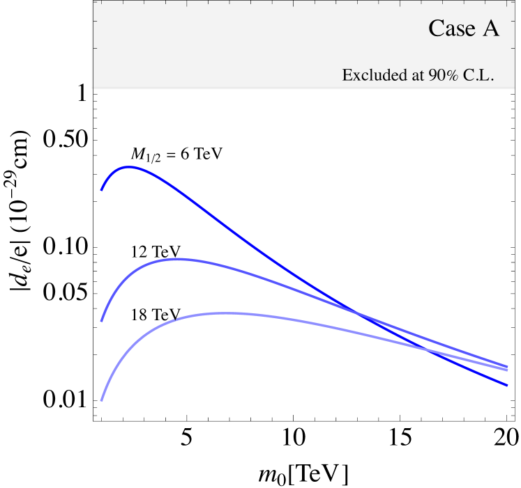
Figure 1: The predicted $|d_{e}/e|$ versus $m_{0}$ with putting $F^{\tau}=m_{0}/2$ in case A. The grey region is excluded by the experimental upper bound.

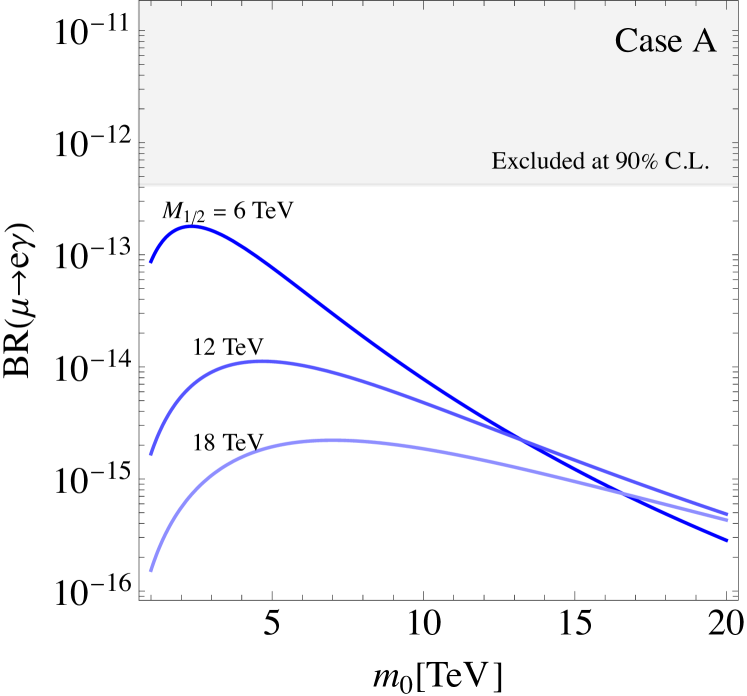
Figure 2: The predicted ${\rm BR}(\mu\to e\gamma)$ versus $m_{0}$ with putting $F^{\tau}=m_{0}/2$ in case A. The grey region is excluded by the experimental upper bound.

At first, we present our numerical results of the electron EDM, $|d_{e}/e|$ for case A. The SUSY mass parameters are variable in $M_{1/2}=6$–$18$ TeV and $m_{0}=1$–$20$ TeV, which are allowed in the slepton, bino and wino searches of the LHC experiments [147, 148]. We plot $|d_{e}/e|$ versus $m_{0}$ in Fig. 2, where $F^{\tau}=m_{0}/2$ is put. Three curved lines correspond to $M_{1/2}=6,\,12,\,18$  TeV, respectively. As seen in Fig. 2, the predicted electron EDM is lower than the experimental upper bound as far as the SUSY mass scale is larger than a few TeV for $F^{\tau}=m_{0}/2$. Indeed, the predicted value is consistent with the experimental upper bound if the gaugino mass scale $M_{1/2}$ is larger than $4$ TeV.

It would be helpful to comment on the behavior of the predicted curves. The maximum values are apparently found at the low $m_{0}$ region. The predicted values increase at $m_{0}$ close to $1$ TeV. This behavior is due to taking $F^{\tau}=m_{0}/2$ in order to reduce the number of free parameters, although $\tilde{m}_{eRL}^{2}$ ($A$-term) is proportional to $F^{\tau}$ and independent $m_{0}$ as seen in Eq. (46). If $F^{\tau}$ is fixed to, for example, $1$ TeV, the prediction becomes a monotonically decreasing function against $m_{0}$.

The SUSY mass scale is also significantly constrained by the experimental upper bound of the branching ratio for the $\mu\rightarrow e\gamma$ decay [74] . We plot ${\rm BR}(\mu\to e\gamma)$ versus $m_{0}$ in Fig. 2, where we put $F^{\tau}=m_{0}/2$ again. It is found that the predicted ${\rm BR}(\mu\to e\gamma)$ is lower than the experimental upper bound as far as the gaugino mass scale $M_{1/2}$ is larger than $6$ TeV. Thus, the $\mu\to e\gamma$ process constrains more severely the SUSY mass scale compared with the electron EDM for case A.

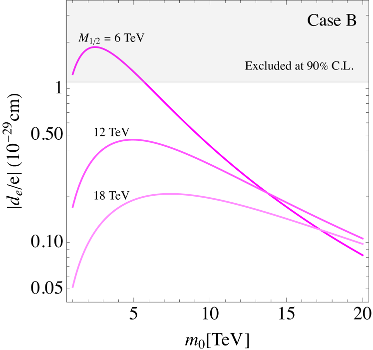
Figure 3: The predicted $|d_{e}/e|$ versus $m_{0}$ with putting $F^{\tau}=m_{0}/2$ in case B. The grey region is excluded by the experimental upper bound.

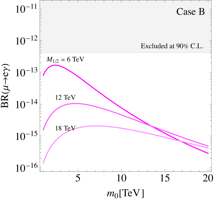
Figure 4: The predicted ${\rm BR}(\mu\to e\gamma)$ versus $m_{0}$ with putting $F^{\tau}=m_{0}/2$ in case B. The grey region is excluded by the experimental upper bound.

In contrast to case A, the electron EDM constrains tightly the SUSY mass scale in case B. We present our numerical results of the electron EDM, $|d_{e}/e|$ and ${\rm BR}(\mu\to e\gamma)$ for case B. We plot $|d_{e}/e|$ versus $m_{0}$ in Fig. 4, where $F^{\tau}=m_{0}/2$ is put. It is found that the predicted electron EDM exceeds the experimental upper bound at $m_{0}\leq 5$ TeV if the gaugino mass scale $M_{1/2}$ is $6$ TeV.

We show ${\rm BR}(\mu\to e\gamma)$ versus $m_{0}$ with putting $F^{\tau}=m_{0}/2$ in Fig. 4. The predicted ${\rm BR}(\mu\to e\gamma)$ is almost same as the one in case A of Fig. 2.

Thus, the constraints of the SUSY mass scale from the upper bounds $|d_{e}/e|$ and ${\rm BR}(\mu\to e\gamma)$ depend on the model of the charged leptons.

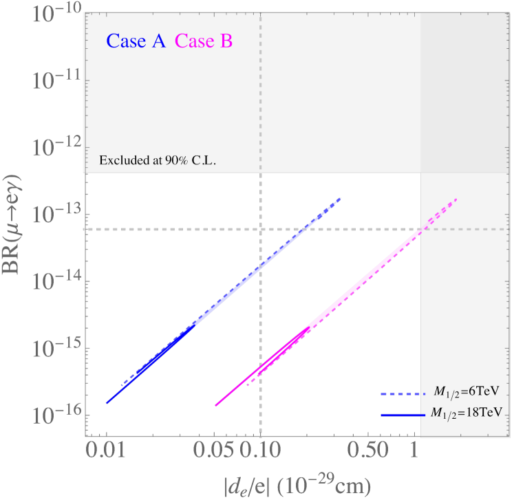
Figure 5: Plot of $|d_{e}/e|$ and ${\rm BR}(\mu\to e\gamma)$ for cases A and B with $F^{\tau}=m_{0}/2$, where $m_{0}=1$–$20$ TeV for fixed $M_{1/2}=6$ and $18$ TeV. The blue curves denotes the predictions at fixed gaugino mass $M_{1/2}$ for case A, and the pink one for case B. The grey regions are excluded by the experimental upper bounds, and the vertical and horizontal dashed grey lines indicate the future sensitivity.

Figure 6: Plot of $|d_{e}/e|$ and ${\rm BR}(\mu\to e\gamma)$ for cases A and B with $F^{\tau}=m_{0}/2$, where $M_{1/2}=6$–$18$ TeV for fixed $m_{0}=1\,,10$ and $20$ TeV. The blue curves denotes the predictions at fixed $m_{0}$ for case A, and the pink one for case B. The grey regions are excluded by the experimental upper bounds, and the vertical and horizontal dashed grey lines indicate the future sensitivity.

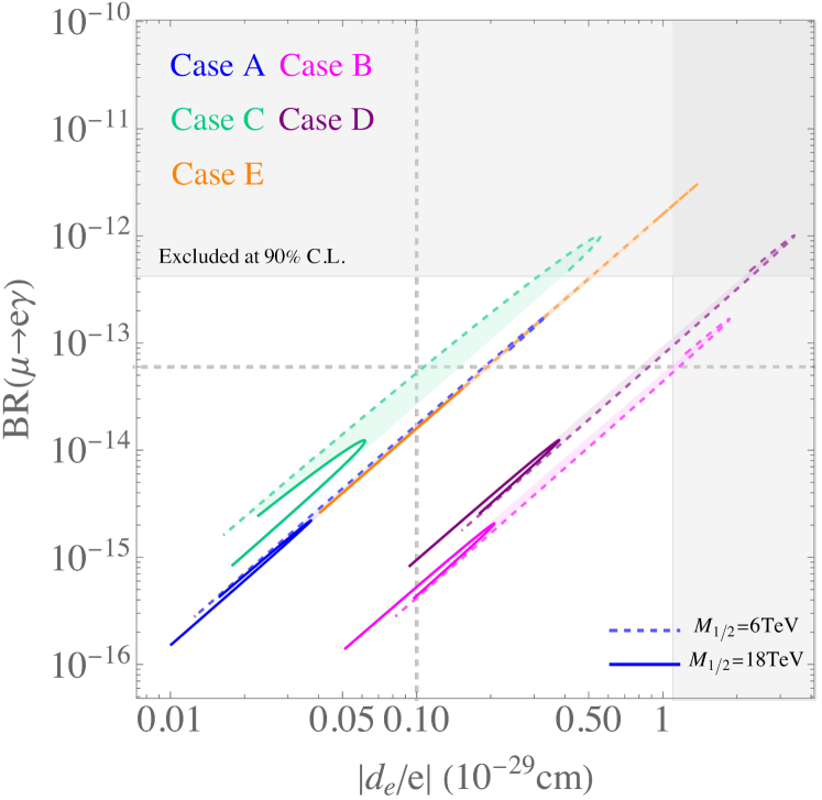
Figure 7: Plot of $|d_{e}/e|$ and ${\rm BR}(\mu\to e\gamma)$ for all cases with $F^{\tau}=m_{0}/2$, where $m_{0}=1$–$20$ TeV for fixed $M_{1/2}=6$ and $18$ TeV. The blue curves denotes the predictions at fixed gaugino mass $M_{1/2}$ for case A, and the same for other cases. The grey regions are excluded by the experimental upper bounds, and the vertical and horizontal dashed grey lines indicate the future sensitivity.

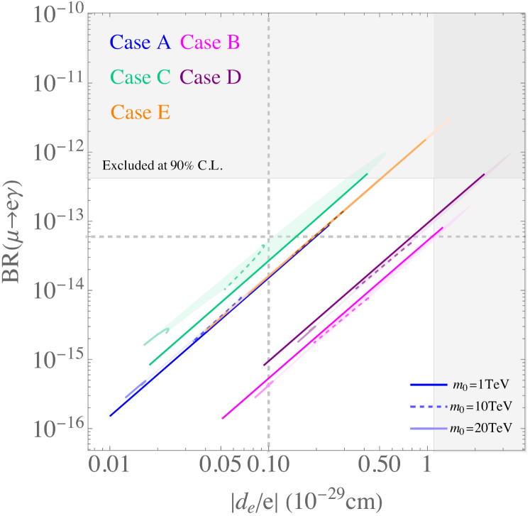
Figure 8: Plot of $|d_{e}/e|$ and ${\rm BR}(\mu\to e\gamma)$ for all cases with $F^{\tau}=m_{0}/2$, where $M_{1/2}=6$–$18$ TeV for fixed $m_{0}=1\,,10$ and $20$ TeV. The blue curves denotes the predictions at fixed $m_{0}$ for case A, and the same for other cases. The grey regions are excluded by the experimental upper bounds, and the vertical and horizontal dashed grey lines indicate the future sensitivity.

In order to see the importance of CP phases via the modulus $\tau$, we examine the correlation between the electron EDM and the decay rate of the $\mu\rightarrow e\gamma$ decay for both cases A and B. The correlation is clearly seen in Figs. 6 and 6. We plot them in the range of $m_{0}=1$–$20$ TeV with fixing $M_{1/2}=6$ and $18$ TeV in Fig. 6, on the other hand, in the range of $M_{1/2}=6$–$18$ TeV with fixing $m_{0}=1$, $10$ and $20$ TeV in Fig. 6.

We find the linear correspondence between ${\rm BR}(\mu\to e\gamma)$ and $|d_{e}/e|$ in the logarithmic coordinates for both cases A and B. The branching ratio is approximately proportional to the square of $|d_{e}/e|$. The slope of the line is independent of the value of $F^{\tau}$, although $F^{\tau}=m_{0}/2$ is taken in these figures. Similar correlations are also found in other cases B–E. This provides a crucial test for our predictions in future. It is also seen that the predicted decay rate of $\mu\rightarrow e\gamma$ is almost same for both cases A and B while the predicted $|d_{e}/e|$ of case B is larger than the one of case A in factor $5$. Thus, the magnitude of the predicted electron EDM depends on the charged lepton mass matrix considerably.

Although the bound of the electron EDM is $|d_{e}/e|\leq 1.1\times 10^{-29}$ cm [116], the future sensitivity is expected to reach up to $|d_{e}/e|\simeq 10^{-30}$ cm [117, 118], which is denoted by the vertical dashed grey line. For case A, their sensitive mass scale is much below $10$ TeV for $m_{0}$ and $M_{1/2}$ as seen in Figs. 6 and 6. On the other hand, for case B, the electron EDM can probe the mass scale $m_{0}$ of $10$–$20$ TeV as seen in Figs. 6 and 6. The future sensitivity of the branching ratio ${\rm BR}(\mu\to e\gamma)$ is $6\times 10^{-14}$ [152], which is shown by the horizontal dashed grey line, excludes only the SUSY mass region much below $10$ TeV.

Let us discuss the model dependence among A–E. We show the correlations between $|d_{e}/e|$ and ${\rm BR}(\mu\to e\gamma)$ for all cases A–E in Figs. 8 and 8. We plot them in the range of $m_{0}=1$–$20$ TeV with fixing $M_{1/2}=6$ and $18$ TeV in Fig. 8, on the other hand, in the range of $M_{1/2}=6$–$18$ TeV with fixing $m_{0}=1$, $10$ and $20$ TeV in Fig. 8. The predicted $|d_{e}/e|$ and ${\rm BR}(\mu\to e\gamma)$ of case A and case C are similar each other, and those of case B and case D are also similar each other as seen in Figs. 8 and 8. The prediction of case E overlaps somewhat with the one of case A, but its region of case E extends upward considerably. The $\mu\to e\gamma$ process of case E constrains most severely the SUSY mass scale among A–E. On the other hand, the electron EDM of case D constrains most severely the SUSY mass scale.

The future sensitivity of the electron EDM, $|d_{e}/e|\simeq 10^{-30}$ cm [117, 118] will probe the SUSY mass scale of $10$–$20$ TeV for B, D and E. On the other hand, the future sensitivity of the branching ratio ${\rm BR}(\mu\to e\gamma)$, $6\times 10^{-14}$ [152] can probe the SUSY mass scale close to $10$ TeV only for case E. For cases A–D, their sensitive mass scale is much below $10$ TeV.

It is noted that the branching ratio of $\mu\to 3e$ and the conversion rate of $\mu N\to eN$ will be sensitive for proving the SUSY mass scale of higher than $10$ TeV although the predicted branching ratio and conversion rate are significantly below the current experimental upper bounds as discussed later [153, 154, 155].

Cases	A	B	C	D	E
$(\delta_{eLR})_{11}\times 10^{8}$	$0.46-0.56\,i$	$1.8+3.0\,i$	$-12-1.0\,i$	$-28-5.6\,i$	$-56-2.2\,i$
$(\delta_{eLR})_{22}\times 10^{5}$	$-1.74+0.42\,i$	$1.0+0.42\,i$	$-1.3-0.39\,i$	$0.62-0.37\,i$	$-0.15-0.95\,i$
$(\delta_{eLR})_{12}\times 10^{6}$	$0.91-4.42\,i$	$-0.83-4.2\,i$	$11-0.60\,i$	$-11-1.0\,i$	$7.4+18\,i$
$(\delta_{eLR})_{13}\times 10^{4}$	$0.46+0.54\,i$	$-0.45+0.55\,i$	$1.5+4.3\,i$	$1.4-3.8\,i$	$0.15-1.9\,i$
$(\delta_{eLR})_{21}\times 10^{7}$	$-0.21+0.04\,i$	$-1.7-0.12\,i$	$0.70-0.13\,i$	$1.0+0.2\,i$	$0.28-0.87\,i$
$(\delta_{eLR})_{23}\times 10^{5}$	$0.65-18\,i$	$-0.53-17\,i$	$-12-30\,i$	$-11+27\,i$	$34.3+2.4\,i$
$(\delta_{eLR})_{31}\times 10^{7}$	$-0.22+0.14\,i$	$-0.10+0.49\,i$	$0.62-0.97\,i$	$-0.10+1.8\,i$	$0.087+0.54\,i$
$(\delta_{eRR})_{21}\times 10^{5}$	$-0.04-0.23\,i$	$-48+21\,i$	$0.19-0.009\,i$	$26+1.4\,i$	$0$
$(\delta_{eRR})_{31}\times 10^{5}$	$-2.99+2.41\,i$	$-0.82+9.2\,i$	$2.2-9.2\,i$	$4.5+14\,i$	$0$
$(\delta_{eRR})_{32}\times 10^{2}$	$0.72+1.3\,i$	$0.7-1.2\,i$	$-0.38+1.2\,i$	$0.39+1.3\,i$	$0$
flavor-conserving $d_{e}/e$ cm	$7.2\times 10^{-31}$	$-3.7\times 10^{-30}$	$1.3\times 10^{-30}$	$7.6\times 10^{-30}$	$2.9\times 10^{-30}$
flavored $d_{e}/e$ cm	$-5.1\times 10^{-32}$	$-2.4\times 10^{-31}$	$-3.9\times 10^{-31}$	$2.5\times 10^{-31}$	$-1.9\times 10^{-37}$
$|\sum d_{e}/e|$ cm	$6.7\times 10^{-31}$	$3.9\times 10^{-30}$	$9.1\times 10^{-31}$	$7.9\times 10^{-30}$	$2.9\times 10^{-30}$
${\rm BR}(\mu\to e\gamma)$	$7.8\times 10^{-15}$	$6.6\times 10^{-15}$	$4.5\times 10^{-14}$	$4.8\times 10^{-14}$	$1.4\times 10^{-13}$
${\rm BR}(\mu\rightarrow ee\bar{e})$	$4.6\times 10^{-17}$	$3.9\times 10^{-17}$	$2.7\times 10^{-16}$	$2.8\times 10^{-16}$	$8.3\times 10^{-16}$
${\rm CR}(\mu N\to eN)$	$5.7\times 10^{-17}$	$4.8\times 10^{-17}$	$3.3\times 10^{-16}$	$3.5\times 10^{-16}$	$1.0\times 10^{-15}$

Table 4: Mass insertion parameters and predicted $d_{e}/e$ (flavor-conserving EDM, flavored one and those sum), ${\rm BR}(\mu\to e\gamma)$, ${\rm BR}(\mu\rightarrow ee\bar{e})$ and ${\rm CR}(\mu N\to eN)$ at $M_{1/2}=6$ TeV, $m_{0}=10$ TeV and $F^{\tau}=5$ TeV.

We have listed predicted mass insertion parameters and $d_{e}/e$, ${\rm BR}(\mu\to e\gamma)$, ${\rm BR}(\mu\rightarrow ee\bar{e})$ and ${\rm CR}(\mu N\to eN)$ at $M_{1/2}=6$ TeV, $m_{0}=10$ TeV and $F^{\tau}=5$ TeV in Table 4. In this setup, the gaugino masses are given as $M_{1}=2.9$ TeV and $M_{2}=5.2$ TeV at $Q=1$ TeV, respectively.

The dominant contribution to the electron EDM comes from the imaginary part of the single chirality flipping diagonal mass insertion $(\delta_{eLR})_{11}$ (flavor-conserving EDM) as seen in Eq. (5.1). Therefore, the flavor-conserving EDM is almost proportional to ${\rm Im}(\delta_{eLR})_{11}$ up to its sign. The small differences of $\tilde{m}_{eR}$ among five cases cause the slight dispersion of the proportionality. The largest flavor-conserving EDM is obtained in case D. The next-to-leading term is the flavored EDM, which arises mainly from the non-vanishing $(\delta_{eRR})_{ij}$. Therefore, it is considerably suppressed in case E since $(\delta_{eRR})_{ij}$ vanish. The largest magnitude of the flavored EDM is obtained in case C. The sum of flavor-conserving EDM and flavored one is in the range of $(0.62$–$7.2)\times 10^{-30}$ cm for all cases. The future experiment can reach up to this range.

We can also calculate the leading contribution of the muon EDM by using $(\delta_{eLR})_{22}$ of Table. 4. It is predicted as:

$$|d_{\mu}/e|\simeq 5\times 10^{-27}\,{\rm cm}\,,$$ (63)

for case A. This predicted value is significantly below its observed upper bound, $2\times 10^{-19}$ at BNL-E821 [118]. The improvement up to $2\times 10^{-21}$ is expected at FNAL [118].

The leading terms of the branching ratio ${\rm BR}(\mu\to e\gamma)$ are given in terms of $(\delta_{eLR})_{12}$ and $(\delta_{eLR})_{12}^{*}$ as seen in Eq. (61) due to the chiral enhancement. The next-to-leading ones arise from $(\delta_{eRR})_{ij}$. However, the contribution of the next-to-leading terms are suppressed enough compared with the leading ones in all cases. The branching ratio is predicted in rather broad range $6.6\times 10^{-15}$–$9.4\times 10^{-14}$ for all cases. Case E will be tested since the future sensitivity is expected to be $6\times 10^{-14}$ [152].

In SUSY models, the branching ratio of $\mu\to 3e$ and the conversion rate of $\mu N\to eN$ are simply related to ${\rm BR}(\mu\to e\gamma)$ as seen in Eq. (62). The five branching ratio and conversion rate are enough below the current experimental upper bounds $1.0\times 10^{-12}$ and $7.0\times 10^{-13}$ [157], respectively, as seen in Table 4. Since future experiments will explore these predictions at the level of $10^{-16}$ for $\mu\to 3e$ and $\mu N\to eN$ [153, 154, 155], it will probe the SUSY mass scale of $m_{0}\simeq 10$ TeV.

We can also calculate the branching ratios of tauon decays, $\tau\rightarrow e\gamma$ and $\tau\rightarrow\mu\gamma$. Both branching ratios are at most ${\cal O}(10^{-13})$, which are much below the current experimental upper bounds $3.3\times 10^{-8}$ and $4.4\times 10^{-8}$, respectively [157].

As well known, large flavor-violating trilinear coupling may generate instabilities of the electroweak vacuum, which constrains the magnitudes of mass insertion parameters $\delta_{eLR}$ [156]. It is noted that our predicted ones do not spoil the vacuum stability.

We also comment on the effect of neutrino Yukawa matrix in the type-I seesaw to the $\mu\to e\gamma$ decay. If there are right-handed neutrinos which couple to the left-handed neutrinos via Yukawa couplings, the RGEs effects, which is the running from the high scale $Q_{0}$ to the right-handed Majorana mass scale $M_{R}$, can also induce off-diagonal elements in the slepton mass matrix as follows [158, 159]:

$$(\delta_{eLL})_{12}\simeq-\frac{6m_{0}^{2}}{16\pi^{2}m_{\rm slepton}^{2}}(Y_{D}^{\dagger}Y_{D})_{12}\ln\frac{Q_{0}}{M_{R}}\,,$$ (64)

where $Y_{D}$ is Dirac neutrino Yukawa matrix in the diagonal base of the charged lepton. One should check its effect to the $\mu\to e\gamma$ decay since our models use type-I seesaw. In conclusion, the effect of neutrino Yukawa couplings is still at the next-to-leading order of our prediction as far as we take $M_{R}\leq 10^{13}$ GeV. For example, in case A, we have

$$(\delta_{eLL})_{12}\simeq 4.9\times 10^{-3}\ (\,6.6\times 10^{-4}\,)\,,\qquad{\rm BR}(\mu\to e\gamma)\simeq 4.8\times 10^{-16}\ (\,8.5\times 10^{-18}\,)\,,$$ (65)

for $M_{R}=10^{13}\,(10^{12})$ GeV, where we take $M_{1}=2.9$ TeV, $M_{2}=5.2$ TeV and $m_{\rm slepton}=m_{0}=10$ TeV, and the branching ratio includes only the contribution of neutrino Yukawa couplings.

In our numerical results, we take $F^{\tau}=m_{0}/2$ to prevent the tachyonic slepton since the largest weight is $k_{\tau}=7$ in our lepton mass matrix. Our predicted electron EDM is almost proportional to the magnitude of $F^{\tau}$, and the branching ratio of $\mu\to e\gamma$ is roughly proportional to $|F^{\tau}|^{2}$ in the following numerical analyses. We have checked the numerical results in the case of $F^{\tau}=m_{0}$ for case E, where tachyonic sleptons are prevented due to small weight $1$. Indeed, the calculated $|d_{e}/e|$ is approximately two times lager than the one for $F^{\tau}=m_{0}/2$, while ${\rm BR}(\mu\to e\gamma)$ is four times lager. Thus, we can estimate roughly $|F^{\tau}|$ dependence of our numerical results.

7 Summary

We have studied the electron EDM in the supersymmetric $\rm A_{4}$ modular invariant theory of flavors with CP invariance. The CP symmetry of the lepton sector is broken by fixing modulus $\tau$. In this framework, a fixed $\tau$ also causes the CP violation in the soft SUSY breaking terms. The electron EDM arises from this CP non-conserved soft SUSY breaking terms. We have examined the electron EDM in the five cases A–E of charged lepton mass matrices, which are completely consistent with observed lepton masses and PMNS mixing angles. It is found that the present upper bound of $|d_{e}/e|\leq 1.1\times 10^{-29}$ excludes the SUSY mass scale, $m_{0}$ and $M_{1/2}$ below $4$–$6$ TeV depending on cases A–E.

The SUSY mass scale is also significantly constrained by considering the experimental upper bound of the branching ratio of the $\mu\to e\gamma$ decay.

In order to see the effect of CP phase in the modulus $\tau$, we examine the correlation between the electron EDM and the decay rate of the $\mu\rightarrow e\gamma$ decay. The correlations are clearly seen in contrast to models of the conventional flavor symmetry. We have found the linear correspondence ${\rm BR}(\mu\to e\gamma)$ between $|d_{e}/e|$ in the logarithmic coordinates for cases A–E. The branching ratio is approximately proportional to the square of $|d_{e}/e|$. The slope of the line is independent of the value of $F^{\tau}$ although $F^{\tau}=m_{0}/2$ is taken in our calculations.

The predicted $d_{e}/e$ and ${\rm BR}(\mu\to e\gamma)$ of case A and case C are similar each other, and those of case B and case D are also similar each other. The $\mu\to e\gamma$ decay constrains most severely the SUSY mass scale in case E compared with other cases. On the other hand, the electron EDM constrains most severely the SUSY mass scale in case D among five cases.

Although the current experimental upper bound of the electron EDM is $|d_{e}/e|\leq 1.1\times 10^{-29}$ cm, the future sensitivity of the electron EDM is expected to reach up to $|d_{e}/e|\simeq 10^{-30}$ cm. Then, the SUSY mass scale will be significantly constrained by $|d_{e}/e|$. Indeed, it will probe the SUSY mass scale of $10$–$20$ TeV.

On the other hand, the future sensitivity of the branching ratio ${\rm BR}(\mu\to e\gamma)$, $6\times 10^{-14}$ probes at most the SUSY mass scale of $10$ TeV. It is also remarked that the branching ratio of $\mu\to 3e$ and the conversion rate of $\mu N\to eN$ will be sensitive for probing the SUSY mass scale of higher than $10$ TeV.

Thus, the electron EDM provides a severe test of the CP violation via the modulus $\tau$ in the supersymmetric modular invariant theory of flavors.

Acknowledgments

We thank Tatsuo Kobayashi for useful discussions. The work of K.Y. was supported by the JSPS KAKENHI 21K13923.

Appendix

Appendix A Tensor product of $\rm A_{4}$ group

We take the generators of $\rm A_{4}$ group for the triplet as follows:

$$\begin{aligned} S=\frac{1}{3}\begin{pmatrix}-1&2&2\\ 2&-1&2\\ 2&2&-1\end{pmatrix},\end{aligned}\qquad\begin{aligned} T=\begin{pmatrix}1&0&0\\ 0&\omega&0\\ 0&0&\omega^{2}\end{pmatrix},\end{aligned}$$ (66)

where $\omega=e^{i\frac{2}{3}\pi}$ for a triplet. In this base, the multiplication rule is

$$\begin{pmatrix}a_{1}\\ a_{2}\\ a_{3}\end{pmatrix}_{\bf 3}\otimes\begin{pmatrix}b_{1}\\ b_{2}\\ b_{3}\end{pmatrix}_{\bf 3} =\left(a_{1}b_{1}+a_{2}b_{3}+a_{3}b_{2}\right)_{\bf 1}\oplus\left(a_{3}b_{3}+a_{1}b_{2}+a_{2}b_{1}\right)_{{\bf 1}^{\prime}}$$

$$\oplus\left(a_{2}b_{2}+a_{1}b_{3}+a_{3}b_{1}\right)_{{\bf 1}^{\prime\prime}}$$

$$\oplus\frac{1}{3}\begin{pmatrix}2a_{1}b_{1}-a_{2}b_{3}-a_{3}b_{2}\\ 2a_{3}b_{3}-a_{1}b_{2}-a_{2}b_{1}\\ 2a_{2}b_{2}-a_{1}b_{3}-a_{3}b_{1}\end{pmatrix}_{{\bf 3}}\oplus\frac{1}{2}\begin{pmatrix}a_{2}b_{3}-a_{3}b_{2}\\ a_{1}b_{2}-a_{2}b_{1}\\ a_{3}b_{1}-a_{1}b_{3}\end{pmatrix}_{{\bf 3}\ }\ ,$$

$${\bf 1}\otimes{\bf 1}={\bf 1}\ ,\qquad {\bf 1^{\prime}}\otimes{\bf 1^{\prime}}={\bf 1^{\prime\prime}}\ ,\qquad{\bf 1^{\prime\prime}}\otimes{\bf 1^{\prime\prime}}={\bf 1^{\prime}}\ ,\qquad{\bf 1^{\prime}}\otimes{\bf 1^{\prime\prime}}={\bf 1}\ ,$$ (67)

where

$$T({\bf 1^{\prime})}=\omega\,,\qquad T({\bf 1^{\prime\prime}})=\omega^{2}.$$ (68)

More details are shown in the review [2, 3].

Appendix B Modular forms with weight 2,  4,  6,  8 in $\Gamma_{3}$ group

We present modular forms with weight 2,  4,  6,  8 in $\rm A_{4}$ modular group. The triplet modular forms can be written in terms of $\eta(\tau)$ and its derivative [11]:

$$Y_{1} = \frac{i}{2\pi}\left(\frac{\eta^{\prime}(\tau/3)}{\eta(\tau/3)}+\frac{\eta^{\prime}((\tau+1)/3)}{\eta((\tau+1)/3)}+\frac{\eta^{\prime}((\tau+2)/3)}{\eta((\tau+2)/3)}-\frac{27\eta^{\prime}(3\tau)}{\eta(3\tau)}\right),$$

$$Y_{2} = \frac{-i}{\pi}\left(\frac{\eta^{\prime}(\tau/3)}{\eta(\tau/3)}+\omega^{2}\frac{\eta^{\prime}((\tau+1)/3)}{\eta((\tau+1)/3)}+\omega\frac{\eta^{\prime}((\tau+2)/3)}{\eta((\tau+2)/3)}\right),$$ (69)

$$Y_{3} = \frac{-i}{\pi}\left(\frac{\eta^{\prime}(\tau/3)}{\eta(\tau/3)}+\omega\frac{\eta^{\prime}((\tau+1)/3)}{\eta((\tau+1)/3)}+\omega^{2}\frac{\eta^{\prime}((\tau+2)/3)}{\eta((\tau+2)/3)}\right)\,.$$

They are also expressed in the $q$ expansions, where $q=e^{i2\pi\tau}$, as follows:

$${\bf Y^{\rm(2)}_{3}}(\tau)=\begin{pmatrix}Y_{1}\\ Y_{2}\\ Y_{3}\end{pmatrix}=\begin{pmatrix}1+12q+36q^{2}+12q^{3}+\dots\\ -6q^{1/3}(1+7q+8q^{2}+\dots)\\ -18q^{2/3}(1+2q+5q^{2}+\dots)\end{pmatrix}.$$ (70)

For weight 4, there are five modular forms by the tensor product of $\bf 3\otimes 3$ as:

For $k=6$, there are seven modular forms by the tensor products of $\rm A_{4}$ as:

For $k=8$, there are 9 modular forms by the tensor products of $\rm A_{4}$ as:

Appendix C RGEs of leptons and slepton

The relevant RGEs are given by [141, 142];

$$\begin{split}16\pi^{2}\frac{d}{dt}\left({\tilde{m}}^{2}_{eL}\right)_{ij}=&-\left(\frac{6}{5}g_{1}^{2}\left|M_{1}\right|^{2}+6g_{2}^{2}\left|M_{2}\right|^{2}\right)\delta_{ij}-\frac{3}{5}g_{1}^{2}~{}S~{}\delta_{ij}\\ &+\left(({\tilde{m}}^{2}_{eL}){Y}_{e}^{\dagger}{Y}_{e}+{Y}_{e}^{\dagger}{Y}_{e}({\tilde{m}}^{2}_{eL})_{K}\right)_{ij}\\ &+2\left({Y}_{e}^{\dagger}({\tilde{m}}^{2}_{eR})_{K}{Y}_{e}+{\tilde{m}}^{2}_{H_{d}}{Y}_{e}^{\dagger}{Y}_{e}+{A}_{e}^{\dagger}{A}_{e}\right)_{ij}\ ,\\ 16\pi^{2}\frac{d}{dt}\left({\tilde{m}}^{2}_{eR}\right)_{ij}=&-\frac{24}{5}g_{1}^{2}\left|M_{1}\right|^{2}\delta_{ij}+\frac{6}{5}g_{1}^{2}~{}S~{}\delta_{ij}\\ &+2\left(({\tilde{m}}^{2}_{eR})_{K}{Y}_{e}{Y}_{e}^{\dagger}+{Y}_{e}{Y}_{e}^{\dagger}({\tilde{m}}^{2}_{eR})_{K}\right)_{ij}\\ &+4\left({Y}_{e}({\tilde{m}}^{2}_{eL})_{K}{Y}_{e}^{\dagger}+{m}^{2}_{H_{d}}{Y}_{e}{Y}_{e}^{\dagger}+{A}_{e}{A}_{e}^{\dagger}\right)_{ij}~{},\\ 16\pi^{2}\frac{d}{dt}\left({A}_{e}\right)_{ij}=&\left(-\frac{9}{5}g_{1}^{2}-3g_{2}^{2}+3{\rm Tr}({Y}_{d}^{\dagger}{Y}_{d})+{\rm Tr}({Y}_{e}^{\dagger}{Y}_{e})\right)\left({A}_{e}\right)_{ij}\\ &+2\left(\frac{9}{5}g_{1}^{2}M_{1}+3g_{2}^{2}M_{2}+3{\rm Tr}({Y}_{d}^{\dagger}{A}_{d})+{\rm Tr}({Y}_{e}^{\dagger}{A}_{e})\right){Y}_{e_{ij}}\\ &+4\left({Y}_{e}{Y}_{e}^{\dagger}{A}_{e}\right)_{ij}+5\left({A}_{e}{Y}_{e}^{\dagger}{Y}_{e}\right)_{ij}~{},\\ 16\pi^{2}\frac{d}{dt}{Y}_{e_{ij}}=&\left(-\frac{9}{5}g_{1}^{2}-3g_{2}^{2}+3\,{\rm Tr}({Y}_{d}{Y}_{d}^{\dagger})+{\rm Tr}({Y}_{e}{Y}_{e}^{\dagger})\right){Y}_{e_{ij}}+3\,\left({Y}_{e}{Y}_{e}^{\dagger}{Y}_{e}\right)_{ij}\ .\end{split}$$ (71)

In these expressions, $g_{1,2}$ are the gauge couplings of SU(2)${}_{L}\times U(1)_{Y}$, $M_{1,2}$ are the corresponding gaugino mass terms, ${Y}_{e,d}$ are the Yukawa couplings for charged leptons and down quarks, ${A}_{e}=({\tilde{m}}^{2}_{eLR})/v_{d}$, and

$$S={\rm Tr}({\tilde{m}}^{2}_{qL}+{\tilde{m}}^{2}_{dR}-2{\tilde{m}}^{2}_{uR}-{\tilde{m}}^{2}_{eL}+{\tilde{m}}^{2}_{eR})-{\tilde{m}}^{2}_{H_{d}}+{\tilde{m}}^{2}_{H_{u}},$$

where ${\tilde{m}}^{2}_{qL}$, ${\tilde{m}}^{2}_{dL}$, ${\tilde{m}}^{2}_{uR}$ are mass matrices of squarks and $\tilde{m}_{H_{u}}$ and $\tilde{m}_{H_{d}}$ are the Higgs masses. The parameter $t$ is $t=\ln Q/Q_{0}$, where $Q$ is the renormalization scale and $Q_{0}$ is a reference scale.

Appendix D Loop functions

The dimensionless functions $C_{B}$, $C^{\prime}_{B,R}$, $C^{\prime}_{B,L}$ and $C^{\prime\prime}_{B}$ are given approximately as [102]:

$$C_{B} \simeq h_{1}(\bar{x})\,,$$ (72)

$$C^{\prime}_{B,R} \simeq C^{\prime}_{B,L}\simeq\frac{1}{2}\,[h_{1}(\bar{x})+k_{1}(\bar{x})]\,,$$ (73)

$$C^{\prime\prime}_{B} \simeq \frac{1}{3}\,[h_{1}(\bar{x})+2\,k_{1}(\bar{x})]\,,$$ (74)

where we take $\tilde{m}_{e}=\sqrt{\tilde{m}_{eL}\tilde{m}_{eR}}$ as the average slepton mass and put $\bar{x}=(M_{1}/\tilde{m}_{e})^{2}$.

On the other hand, functions $C^{\prime}_{L}$, $C^{\prime}_{R}$ and $C^{\prime}_{2}$ are exactly given as:

$$C^{\prime}_{L} = C_{0}\frac{1}{m_{eL}^{2}}\frac{y_{L}}{y_{L}-x_{L}}\left[\,h_{1}\left(x_{L}\right)-\,h_{1}\left(y_{L}\right)\right],$$ (76)

$$C^{\prime}_{R} = C_{0}\frac{1}{m_{eR}^{2}}\frac{y_{R}}{y_{R}-x_{R}}\left[\,h_{1}\left(x_{R}\right)-\,h_{1}\left(y_{R}\right)\right],$$ (77)

$$C^{\prime}_{2} = C_{0}\frac{M_{2}\cot^{2}\theta_{W}}{M_{1}m_{eL}^{2}}\frac{y_{L}}{y_{L}-x^{\prime}_{L}}\left[\,h_{2}\left(x^{\prime}_{L}\right)-\,h_{2}\left(y_{L}\right)\right],$$ (78)

with

$$x_{L}=\frac{M_{1}^{2}}{m_{eL}^{2}}\,,~{}~{}\quad x_{R}=\frac{M_{1}^{2}}{m_{eR}^{2}}\,,~{}~{}\quad x^{\prime}_{L}=\frac{M_{2}^{2}}{m_{eL}^{2}}\,,~{}~{}\quad y_{L}=\frac{\mu^{2}}{m_{eL}^{2}}\,,~{}~{}\quad y_{R}=\frac{\mu^{2}}{m_{eR}^{2}}\,,$$ (80)

where $C_{0}=m_{0}^{4}/\mu^{2}$. Functions $h_{1}(x)$, $h_{2}(x)$ and $k_{1}(x)$ are defined as:

$$h_{1}(x) = \frac{1+4x-5x^{2}+(2x^{2}+4x)\ln x}{(1-x)^{4}}\,,$$ (81)

$$h_{2}(x) = \frac{7x^{2}+4x-11-2(x^{2}+6x+2)\ln x}{2(x-1)^{4}}\,,$$ (82)

$$k_{1}(x) = \frac{d}{dx}[x\,h_{1}(x)]\,.$$ (83)

Note that $M_{i}$ and $\mu^{2}$ are real positive values.

Appendix E Mass matrix $M_{e}$ with only weight 2 modular forms

We present the charged lepton mass matrix in terms of only weight 2 modular forms, in which ${\rm BR}(\mu\to e\gamma)$ was discussed in Ref. [74]. The mass matrix is given as:

$$\begin{aligned} M_{e}=v_{d}\begin{pmatrix}\alpha_{e}&0&0\\ 0&\beta_{e}&0\\ 0&0&\gamma_{e}\end{pmatrix}\begin{pmatrix}Y_{1}&Y_{3}&Y_{2}\\ Y_{2}&Y_{1}&Y_{3}\\ Y_{3}&Y_{2}&Y_{1}\end{pmatrix}\,,\end{aligned}$$ (84)

where $Y_{i}$’s are given in Eq. (B). The neutrino mass matrix is given by the dimension five Weinberg operator. We present the best fit parameter set for the observed lepton masses and flavor mixing angles [68] as follows:

$$E\,:\ \ \tau=-0.0796+1.0065\,i\,,\qquad\alpha_{e}/\gamma_{e}=6.82\times 10^{-2}\,,\qquad\beta_{e}/\gamma_{e}=1.02\times 10^{-3}\,,$$ (85)

which is referred as the case E in the text.

The slepton mass matrix $\tilde{m}^{2}_{eRL}$ including RGE effect is written as:

$$\tilde{m}^{2}_{eRL}\simeq 1.4\,v_{d}\left[-m_{F}\begin{pmatrix}\alpha_{e}&0&0\\ 0&\beta_{e}&0\\ 0&0&\gamma_{e}\end{pmatrix}\begin{pmatrix}Y_{1}&Y_{3}&Y_{2}\\ Y_{2}&Y_{1}&Y_{3}\\ Y_{3}&Y_{2}&Y_{1}\\ \end{pmatrix}+F^{\tau}\begin{pmatrix}\alpha_{e}&0&0\\ 0&\beta_{e}&0\\ 0&0&\gamma_{e}\end{pmatrix}\frac{d}{d\tau}\begin{pmatrix}Y_{1}&Y_{3}&Y_{2}\\ Y_{2}&Y_{1}&Y_{3}\\ Y_{3}&Y_{2}&Y_{1}\\ \end{pmatrix}\right]\,.$$ (86)

Since the first term of the right-hand side is proportional to $M_{e}$, it does not contributes to $|d_{e}/e|$ and ${\rm BR}(\mu\to e\gamma)$. On the other hand, $\tilde{m}^{2}_{eLL}$ and $\tilde{m}^{2}_{eRR}$ are proportional to the unit matrix. Then, these mass terms do not contribute to $|d_{e}/e|$ and ${\rm BR}(\mu\to e\gamma)$.

References

• [1] G. Altarelli and F. Feruglio, Rev. Mod. Phys.  82 (2010) 2701 [arXiv:1002.0211 [hep-ph]].
• [2] H. Ishimori, T. Kobayashi, H. Ohki, Y. Shimizu, H. Okada and M. Tanimoto, Prog. Theor. Phys. Suppl.  183 (2010) 1 [arXiv:1003.3552 [hep-th]].
• [3] H. Ishimori, T. Kobayashi, H. Ohki, H. Okada, Y. Shimizu and M. Tanimoto, Lect. Notes Phys.  858 (2012) 1, Springer.
• [4] D. Hernandez and A. Y. Smirnov, Phys. Rev. D 86 (2012) 053014 [arXiv:1204.0445 [hep-ph]].
• [5] S. F. King and C. Luhn, Rept. Prog. Phys.  76 (2013) 056201 [arXiv:1301.1340 [hep-ph]].
• [6] S. F. King, A. Merle, S. Morisi, Y. Shimizu and M. Tanimoto, New J. Phys.  16, 045018 (2014) [arXiv:1402.4271 [hep-ph]].
• [7] M. Tanimoto, AIP Conf. Proc.  1666 (2015) 120002.
• [8] S. F. King, Prog. Part. Nucl. Phys.  94 (2017) 217 [arXiv:1701.04413 [hep-ph]].
• [9] S. T. Petcov, Eur. Phys. J. C 78 (2018) no.9, 709 [arXiv:1711.10806 [hep-ph]].
• [10] F. Feruglio and A. Romanino, arXiv:1912.06028 [hep-ph].
• [11] F. Feruglio, in From My Vast Repertoire …: Guido Altarelli’s Legacy, A. Levy, S. Forte, Stefano, and G. Ridolfi, eds., pp.227–266, 2019, arXiv:1706.08749 [hep-ph].
• [12] R. de Adelhart Toorop, F. Feruglio and C. Hagedorn, Nucl. Phys. B 858, 437 (2012) [arXiv:1112.1340 [hep-ph]].
• [13] T. Kobayashi, K. Tanaka and T. H. Tatsuishi, Phys. Rev. D 98 (2018) no.1, 016004 [arXiv:1803.10391 [hep-ph]].
• [14] J. T. Penedo and S. T. Petcov, Nucl. Phys. B 939 (2019) 292 [arXiv:1806.11040 [hep-ph]].
• [15] P. P. Novichkov, J. T. Penedo, S. T. Petcov and A. V. Titov, JHEP 1904 (2019) 174 [arXiv:1812.02158 [hep-ph]].
• [16] J. C. Criado and F. Feruglio, SciPost Phys.  5 (2018) no.5, 042 [arXiv:1807.01125 [hep-ph]].
• [17] T. Kobayashi, N. Omoto, Y. Shimizu, K. Takagi, M. Tanimoto and T. H. Tatsuishi, JHEP 1811 (2018) 196 [arXiv:1808.03012 [hep-ph]].
• [18] G. J. Ding, S. F. King and X. G. Liu, JHEP 1909 (2019) 074 [arXiv:1907.11714 [hep-ph]].
• [19] P. P. Novichkov, J. T. Penedo, S. T. Petcov and A. V. Titov, JHEP 1904 (2019) 005 [arXiv:1811.04933 [hep-ph]].
• [20] T. Kobayashi, Y. Shimizu, K. Takagi, M. Tanimoto and T. H. Tatsuishi, JHEP 02 (2020), 097 [arXiv:1907.09141 [hep-ph]].
• [21] X. Wang and S. Zhou, JHEP 05 (2020), 017 [arXiv:1910.09473 [hep-ph]].
• [22] G. J. Ding, S. F. King and X. G. Liu, Phys. Rev. D 100 (2019) no.11, 115005 [arXiv:1903.12588 [hep-ph]].
• [23] X. G. Liu and G. J. Ding, JHEP 1908 (2019) 134 [arXiv:1907.01488 [hep-ph]].
• [24] P. Chen, G. J. Ding, J. N. Lu and J. W. F. Valle, Phys. Rev. D 102 (2020) no.9, 095014 [arXiv:2003.02734 [hep-ph]].
• [25] P. P. Novichkov, J. T. Penedo and S. T. Petcov, Nucl. Phys. B 963 (2021), 115301 [arXiv:2006.03058 [hep-ph]].
• [26] X. G. Liu, C. Y. Yao and G. J. Ding, Phys. Rev. D 103 (2021) no.5, 056013 [arXiv:2006.10722 [hep-ph]].
• [27] I. de Medeiros Varzielas, S. F. King and Y. L. Zhou, Phys. Rev. D 101 (2020) no.5, 055033 [arXiv:1906.02208 [hep-ph]].
• [28] G. J. Ding, S. F. King, C. C. Li and Y. L. Zhou, JHEP 08 (2020), 164 [arXiv:2004.12662 [hep-ph]].
• [29] T. Asaka, Y. Heo, T. H. Tatsuishi and T. Yoshida, JHEP 2001 (2020) 144 [arXiv:1909.06520 [hep-ph]].
• [30] T. Asaka, Y. Heo and T. Yoshida, Phys. Lett. B 811 (2020), 135956 [arXiv:2009.12120 [hep-ph]].
• [31] M. K. Behera, S. Mishra, S. Singirala and R. Mohanta, [arXiv:2007.00545 [hep-ph]].
• [32] S. Mishra, [arXiv:2008.02095 [hep-ph]].
• [33] F. J. de Anda, S. F. King and E. Perdomo, Phys. Rev. D 101 (2020) no.1, 015028 [arXiv:1812.05620 [hep-ph]].
• [34] T. Kobayashi, Y. Shimizu, K. Takagi, M. Tanimoto and T. H. Tatsuishi, arXiv:1906.10341 [hep-ph].
• [35] P. P. Novichkov, S. T. Petcov and M. Tanimoto, Phys. Lett. B 793 (2019) 247 [arXiv:1812.11289 [hep-ph]].
• [36] T. Kobayashi, Y. Shimizu, K. Takagi, M. Tanimoto, T. H. Tatsuishi and H. Uchida, Phys. Lett. B 794 (2019) 114 [arXiv:1812.11072 [hep-ph]].
• [37] H. Okada and M. Tanimoto, Phys. Lett. B 791 (2019) 54 [arXiv:1812.09677 [hep-ph]].
• [38] H. Okada and M. Tanimoto, Eur. Phys. J. C 81 (2021) no.1, 52 [arXiv:1905.13421 [hep-ph]].
• [39] T. Nomura and H. Okada, Phys. Lett. B 797 (2019) 134799 [arXiv:1904.03937 [hep-ph]].
• [40] H. Okada and Y. Orikasa, Phys. Rev. D 100 (2019) no.11, 115037 [arXiv:1907.04716 [hep-ph]].
• [41] Y. Kariyazono, T. Kobayashi, S. Takada, S. Tamba and H. Uchida, Phys. Rev. D 100 (2019) no.4, 045014 [arXiv:1904.07546 [hep-th]].
• [42] T. Nomura and H. Okada, Nucl. Phys. B 966 (2021), 115372 [arXiv:1906.03927 [hep-ph]].
• [43] H. Okada and Y. Orikasa, arXiv:1908.08409 [hep-ph].
• [44] T. Nomura, H. Okada and O. Popov, Phys. Lett. B 803 (2020) 135294 [arXiv:1908.07457 [hep-ph]].
• [45] J. C. Criado, F. Feruglio and S. J. D. King, JHEP 2002 (2020) 001 [arXiv:1908.11867 [hep-ph]].
• [46] S. F. King and Y. L. Zhou, Phys. Rev. D 101 (2020) no.1, 015001 [arXiv:1908.02770 [hep-ph]].
• [47] G. J. Ding, S. F. King, X. G. Liu and J. N. Lu, JHEP 1912 (2019) 030 [arXiv:1910.03460 [hep-ph]].
• [48] I. de Medeiros Varzielas, M. Levy and Y. L. Zhou, JHEP 11 (2020), 085 [arXiv:2008.05329 [hep-ph]].
• [49] D. Zhang, Nucl. Phys. B 952 (2020) 114935 [arXiv:1910.07869 [hep-ph]].
• [50] T. Nomura, H. Okada and S. Patra, Nucl. Phys. B 967 (2021), 115395 [arXiv:1912.00379 [hep-ph]].
• [51] T. Kobayashi, T. Nomura and T. Shimomura, Phys. Rev. D 102 (2020) no.3, 035019 [arXiv:1912.00637 [hep-ph]].
• [52] J. N. Lu, X. G. Liu and G. J. Ding, Phys. Rev. D 101 (2020) no.11, 115020 [arXiv:1912.07573 [hep-ph]].
• [53] X. Wang, Nucl. Phys. B 957 (2020), 115105 [arXiv:1912.13284 [hep-ph]].
• [54] S. J. D. King and S. F. King, JHEP 09 (2020), 043 [arXiv:2002.00969 [hep-ph]].
• [55] M. Abbas, Phys. Rev. D 103 (2021) no.5, 056016 [arXiv:2002.01929 [hep-ph]].
• [56] H. Okada and Y. Shoji, Phys. Dark Univ. 31 (2021), 100742 [arXiv:2003.11396 [hep-ph]].
• [57] H. Okada and Y. Shoji, Nucl. Phys. B 961 (2020), 115216 [arXiv:2003.13219 [hep-ph]].
• [58] G. J. Ding and F. Feruglio, JHEP 06 (2020), 134 [arXiv:2003.13448 [hep-ph]].
• [59] T. Nomura and H. Okada, [arXiv:2007.04801 [hep-ph]].
• [60] T. Nomura and H. Okada, arXiv:2007.15459 [hep-ph].
• [61] H. Okada and M. Tanimoto, [arXiv:2005.00775 [hep-ph]].
• [62] H. Okada and M. Tanimoto, Phys. Rev. D 103 (2021) no.1, 015005 [arXiv:2009.14242 [hep-ph]].
• [63] K. I. Nagao and H. Okada, JCAP 05 (2021), 063 [arXiv:2008.13686 [hep-ph]].
• [64] K. I. Nagao and H. Okada, [arXiv:2010.03348 [hep-ph]].
• [65] C. Y. Yao, X. G. Liu and G. J. Ding, Phys. Rev. D 103, no.9, 095013 (2021) [arXiv:2011.03501 [hep-ph]].
• [66] X. Wang, B. Yu and S. Zhou, Phys. Rev. D 103 (2021) no.7, 076005 [arXiv:2010.10159 [hep-ph]].
• [67] M. Abbas, Phys. Atom. Nucl. 83 (2020) no.5, 764-769.
• [68] H. Okada and M. Tanimoto, JHEP 03 (2021), 010 [arXiv:2012.01688 [hep-ph]].
• [69] C. Y. Yao, J. N. Lu and G. J. Ding, [arXiv:2012.13390 [hep-ph]].
• [70] F. Feruglio, V. Gherardi, A. Romanino and A. Titov, JHEP 05, 242 (2021) [arXiv:2101.08718 [hep-ph]].
• [71] S. F. King and Y. L. Zhou, JHEP 04 (2021), 291 [arXiv:2103.02633 [hep-ph]].
• [72] P. Chen, G. J. Ding and S. F. King, JHEP 04 (2021), 239 [arXiv:2101.12724 [hep-ph]].
• [73] X. Du and F. Wang, [arXiv:2012.01397 [hep-ph]].
• [74] T. Kobayashi, T. Shimomura and M. Tanimoto, [arXiv:2102.10425 [hep-ph]].
• [75] P. P. Novichkov, J. T. Penedo and S. T. Petcov, JHEP 04, 206 (2021) [arXiv:2102.07488 [hep-ph]].
• [76] G. J. Ding, S. F. King and C. Y. Yao, [arXiv:2103.16311 [hep-ph]].
• [77] H. Kuranaga, H. Ohki and S. Uemura, [arXiv:2105.06237 [hep-ph]].
• [78] T. Kobayashi and S. Tamba, Phys. Rev. D 99 (2019) no.4, 046001 [arXiv:1811.11384 [hep-th]].
• [79] A. Baur, H. P. Nilles, A. Trautner and P. K. S. Vaudrevange, Phys. Lett. B 795 (2019) 7 [arXiv:1901.03251 [hep-th]].
• [80] T. Kobayashi, Y. Shimizu, K. Takagi, M. Tanimoto and T. H. Tatsuishi, Phys. Rev. D 100 (2019) no.11, 115045, Erratum: [Phys. Rev. D 101 (2020) no.3, 039904] [arXiv:1909.05139 [hep-ph]].
• [81] H. P. Nilles, S. Ramos-Śanchez and P. K. S. Vaudrevange, JHEP 02 (2020), 045 [arXiv:2001.01736 [hep-ph]].
• [82] H. P. Nilles, S. Ramos-Sánchez and P. K. S. Vaudrevange, Nucl. Phys. B 957 (2020), 115098 [arXiv:2004.05200 [hep-ph]].
• [83] K. Ishiguro, T. Kobayashi and H. Otsuka, [arXiv:2010.10782 [hep-th]].
• [84] S. Kikuchi, T. Kobayashi, S. Takada, T. H. Tatsuishi and H. Uchida, Phys. Rev. D 102 (2020) no.10, 105010 [arXiv:2005.12642 [hep-th]].
• [85] S. Kikuchi, T. Kobayashi, H. Otsuka, S. Takada and H. Uchida, JHEP 11 (2020), 101 [arXiv:2007.06188 [hep-th]].
• [86] T. Kobayashi and H. Otsuka, Phys. Rev. D 102 (2020) no.2, 026004 [arXiv:2004.04518 [hep-th]].
• [87] G. J. Ding, F. Feruglio and X. G. Liu, JHEP 01 (2021), 037 [arXiv:2010.07952 [hep-th]].
• [88] K. Ishiguro, T. Kobayashi and H. Otsuka, JHEP 03 (2021), 161 [arXiv:2011.09154 [hep-ph]].
• [89] T. Kobayashi, Y. Shimizu, K. Takagi, M. Tanimoto, T. H. Tatsuishi and H. Uchida, Phys. Rev. D 101 (2020) no.5, 055046 [arXiv:1910.11553 [hep-ph]].
• [90] K. Hoshiya, S. Kikuchi, T. Kobayashi, Y. Ogawa and H. Uchida, PTEP 2021 (2021) no.3, 033B05 [arXiv:2012.00751 [hep-th]].
• [91] S. Kikuchi, T. Kobayashi and H. Uchida, [arXiv:2101.00826 [hep-th]].
• [92] G. J. Ding, F. Feruglio and X. G. Liu, SciPost Phys. 10 (2021), 133 [arXiv:2102.06716 [hep-ph]].
• [93] H. P. Nilles, S. Ramos–Sánchez and P. K. S. Vaudrevange, Phys. Lett. B 808 (2020), 135615 [arXiv:2006.03059 [hep-th]].
• [94] A. Baur, M. Kade, H. P. Nilles, S. Ramos-Sanchez and P. K. S. Vaudrevange, JHEP 02 (2021), 018 [arXiv:2008.07534 [hep-th]].
• [95] H. P. Nilles, S. Ramos–Sánchez and P. K. S. Vaudrevange, Nucl. Phys. B 966 (2021), 115367 [arXiv:2010.13798 [hep-th]].
• [96] A. Baur, M. Kade, H. P. Nilles, S. Ramos-Sanchez and P. K. S. Vaudrevange, Phys. Lett. B 816 (2021), 136176 [arXiv:2012.09586 [hep-th]].
• [97] A. Baur, M. Kade, H. P. Nilles, S. Ramos-Sánchez and P. K. S. Vaudrevange, [arXiv:2104.03981 [hep-th]].
• [98] P. Ko, T. Kobayashi, J. h. Park and S. Raby, Phys. Rev. D 76, 035005 (2007) [erratum: Phys. Rev. D 76, 059901 (2007)] [arXiv:0704.2807 [hep-ph]].
• [99] H. Ishimori, T. Kobayashi, H. Ohki, Y. Omura, R. Takahashi and M. Tanimoto, Phys. Rev. D 77, 115005 (2008) [arXiv:0803.0796 [hep-ph]].
• [100] H. Ishimori, T. Kobayashi, Y. Omura and M. Tanimoto, JHEP 12, 082 (2008) [arXiv:0807.4625 [hep-ph]].
• [101] H. Ishimori, T. Kobayashi, H. Okada, Y. Shimizu and M. Tanimoto, JHEP 12, 054 (2009) [arXiv:0907.2006 [hep-ph]].
• [102] M. Dimou, S. F. King and C. Luhn, Phys. Rev. D 93, no.7, 075026 (2016) doi:10.1103/PhysRevD.93.075026 [arXiv:1512.09063 [hep-ph]].
• [103] V. S. Kaplunovsky and J. Louis, Phys. Lett. B 306, 269-275 (1993) [arXiv:hep-th/9303040 [hep-th]].
• [104] A. Brignole, L. E. Ibanez and C. Munoz, Nucl. Phys. B 422, 125-171 (1994) [erratum: Nucl. Phys. B 436, 747-748 (1995)] [arXiv:hep-ph/9308271 [hep-ph]].
• [105] T. Kobayashi, D. Suematsu, K. Yamada and Y. Yamagishi, Phys. Lett. B 348, 402-410 (1995) [arXiv:hep-ph/9408322 [hep-ph]].
• [106] L. E. Ibanez, C. Munoz and S. Rigolin, Nucl. Phys. B 553, 43-80 (1999) [arXiv:hep-ph/9812397 [hep-ph]].
• [107] P. P. Novichkov, J. T. Penedo, S. T. Petcov and A. V. Titov, JHEP 1907 (2019) 165 [arXiv:1905.11970 [hep-ph]].
• [108] G. Ecker, W. Grimus and W. Konetschny, Nucl. Phys. B 191 (1981), 465-492.
• [109] G. Ecker, W. Grimus and H. Neufeld, Nucl. Phys. B 247 (1984), 70-82.
• [110] G. Ecker, W. Grimus and H. Neufeld, J. Phys. A 20 (1987), L807.
• [111] H. Neufeld, W. Grimus and G. Ecker, Int. J. Mod. Phys. A 3 (1988), 603-616.
• [112] W. Grimus and M. N. Rebelo, Phys. Rept. 281 (1997), 239-308 [arXiv:hep-ph/9506272 [hep-ph]].
• [113] W. Grimus and L. Lavoura, Phys. Lett. B 579 (2004) 113. [hep-ph/0305309].
• [114] Z. Maki, M. Nakagawa and S. Sakata, Prog. Theor. Phys.  28 (1962) 870.
• [115] B. Pontecorvo, Sov. Phys. JETP 26 (1968) 984 [Zh. Eksp. Teor. Fiz.  53 (1967) 1717].
• [116] V. Andreev et al. [ACME], Nature 562 (2018) no.7727, 355-360.
• [117] D. M. Kara, I. J. Smallman, J. J. Hudson, B. E. Sauer, M. R. Tarbutt and E. A. Hinds, New J. Phys. 14 (2012), 103051 [arXiv:1208.4507 [physics.atom-ph]].
• [118] W. C. Griffith, Plenary talk at ”Interplay between Particle & Astroparticle physics 2014”, https://indico.ph.qmul.ac.uk/indico/conferenceDisplay.py?confId=1.
• [119] M. Fujiwara, J. Hisano, C. Kanai and T. Toma, JHEP 04 (2021), 114 [arXiv:2012.14585 [hep-ph]].
• [120] M. Fujiwara, J. Hisano and T. Toma, [arXiv:2106.03384 [hep-ph]].
• [121] E. Ma and G. Rajasekaran, Phys. Rev.  D 64, 113012 (2001) [arXiv:hep-ph/0106291].
• [122] K. S. Babu, E. Ma and J. W. F. Valle, Phys. Lett.  B 552, 207 (2003) [arXiv:hep-ph/0206292].
• [123] G. Altarelli and F. Feruglio, Nucl. Phys. B 720 (2005) 64 [hep-ph/0504165].
• [124] G. Altarelli and F. Feruglio, Nucl. Phys. B 741 (2006) 215 [hep-ph/0512103].
• [125] Y. Shimizu, M. Tanimoto and A. Watanabe, Prog. Theor. Phys.  126 (2011) 81 [arXiv:1105.2929 [hep-ph]].
• [126] S. T. Petcov and A. V. Titov, Phys. Rev. D 97 (2018) no.11, 115045 [arXiv:1804.00182 [hep-ph]].
• [127] S. K. Kang, Y. Shimizu, K. Takagi, S. Takahashi and M. Tanimoto, PTEP 2018, no. 8, 083B01 (2018) [arXiv:1804.10468 [hep-ph]].
• [128] H. Okada, Y. Shimizu, M. Tanimoto and T. Yoshida, [arXiv:2105.14292 [hep-ph]].
• [129] A. M. Baldini et al. [MEG], Eur. Phys. J. C 76 (2016) no.8, 434 doi:10.1140/epjc/s10052-016-4271-x [arXiv:1605.05081 [hep-ex]].
• [130] F. Feruglio, C. Hagedorn, Y. Lin and L. Merlo, Nucl. Phys. B 832, 251-288 (2010) [arXiv:0911.3874 [hep-ph]].
• [131] H. Ishimori and M. Tanimoto, Prog. Theor. Phys. 125 (2011), 653-675 [arXiv:1012.2232 [hep-ph]].
• [132] G. C. Branco, R. G. Felipe and F. R. Joaquim, Rev. Mod. Phys.  84 (2012) 515 [arXiv:1111.5332 [hep-ph]].
• [133] M. Holthausen, M. Lindner and M. A. Schmidt, JHEP 1304 (2013) 122 [arXiv:1211.6953 [hep-ph]].
• [134] M. C. Chen, M. Fallbacher, K. T. Mahanthappa, M. Ratz and A. Trautner, Nucl. Phys. B 883 (2014) 267 [arXiv:1402.0507 [hep-ph]].
• [135] F. Feruglio, C. Hagedorn and R. Ziegler, JHEP 07 (2013), 027 [arXiv:1211.5560 [hep-ph]].
• [136] S. Ferrara, D. Lust, A. D. Shapere and S. Theisen, Phys. Lett. B 225, 363 (1989).
• [137] M. Chen, S. Ramos-Sánchez and M. Ratz, Phys. Lett. B 801 (2020), 135153 [arXiv:1909.06910 [hep-ph]].
• [138] R. C. Gunning, Lectures on Modular Forms (Princeton University Press, Princeton, NJ, 1962).
• [139] B. Schoeneberg, Elliptic Modular Functions (Springer-Verlag, 1974).
• [140] N. Koblitz, Introduction to Elliptic Curves and Modular Forms (Springer-Verlag, 1984).
• [141] S. P. Martin and M. T. Vaughn, Phys. Rev.  D 50, 2282 (1994) [Erratum-ibid.  D 78, 039903 (2008)] [arXiv:hep-ph/9311340].
• [142] S. P. Martin, Adv. Ser. Direct. High Energy Phys. 18 (1998), 1-98 [arXiv:hep-ph/9709356 [hep-ph]].
• [143] J. Hisano, M. Nagai and P. Paradisi, Phys. Rev.  D 78, 075019 (2008) [arXiv:0712.1285 [hep-ph]].
• [144] F. Borzumati and A. Masiero, Phys. Rev. Lett.  57, 961 (1986).
• [145] F. Gabbiani, E. Gabrielli, A. Masiero and L. Silvestrini, Nucl. Phys.  B 477, 321 (1996) [arXiv:hep-ph/9604387].
• [146] W. Altmannshofer, A. J. Buras, S. Gori, P. Paradisi and D. M. Straub, Nucl. Phys. B 830 (2010), 17-94 [arXiv:0909.1333 [hep-ph]].
• [147] U. Sarkar [CMS], [arXiv:2105.01629 [hep-ex]].
• [148] A. Kalogeropoulos [ATLAS and CMS], PoS LHCP2020 (2021), 166.
• [149] I. Esteban, M. C. Gonzalez-Garcia, M. Maltoni, T. Schwetz and A. Zhou, JHEP 09 (2020), 178 [arXiv:2007.14792 [hep-ph]].
• [150] S. Antusch and V. Maurer, JHEP 1311 (2013) 115 [arXiv:1306.6879 [hep-ph]].
• [151] F. Björkeroth, F. J. de Anda, I. de Medeiros Varzielas and S. F. King, JHEP 1506 (2015) 141 [arXiv:1503.03306 [hep-ph]].
• [152] A. M. Baldini et al. [MEG II], Eur. Phys. J. C 78 (2018) no.5, 380 [arXiv:1801.04688 [physics.ins-det]].
• [153] A. Blondel, A. Bravar, M. Pohl, S. Bachmann, N. Berger, M. Kiehn, A. Schoning, D. Wiedner, B. Windelband and P. Eckert, et al. [arXiv:1301.6113 [physics.ins-det]].
• [154] R. J. Abrams et al. [Mu2e], [arXiv:1211.7019 [physics.ins-det]].
• [155] R. Abramishvili et al. [COMET], PTEP 2020 (2020) no.3, 033C01 [arXiv:1812.09018 [physics.ins-det]].
• [156] J. h. Park, Phys. Rev. D 83 (2011), 055015 doi:10.1103/PhysRevD.83.055015 [arXiv:1011.4939 [hep-ph]].
• [157] P. A. Zyla et al. [Particle Data Group], PTEP 2020 (2020) no.8, 083C01.
• [158] J. Hisano, T. Moroi, K. Tobe, M. Yamaguchi and T. Yanagida, Phys. Lett.  B 357, 579 (1995) [arXiv:hep-ph/9501407].
• [159] J. Hisano, T. Moroi, K. Tobe and M. Yamaguchi, Phys. Rev.  D 53, 2442 (1996) [arXiv:hep-ph/9510309].