Approximation capabilities of measure-preserving neural networks

Abstract

Measure-preserving neural networks are well-developed invertible models, however, their approximation capabilities remain unexplored. This paper rigorously analyses the approximation capabilities of existing measure-preserving neural networks including NICE and RevNets. It is shown that for compact $U\subset\mathbb{R}^{D}$ with $D\geq 2$, the measure-preserving neural networks are able to approximate arbitrary measure-preserving map $\psi:U\to\mathbb{R}^{D}$ which is bounded and injective in the $L^{p}$-norm. In particular, any continuously differentiable injective map with $\pm 1$ determinant of Jacobian are measure-preserving, thus can be approximated.

1 Introduction

Deep neural networks have become an increasingly successful tool in modern machine learning applications and yielded transformative advances across diverse scientific disciplines (Krizhevsky et al., 2017; LeCun et al., 2015; Lu et al., 2021b; Schmidhuber, 2015). It is well known that fully connected neural networks can approximate continuous mappings (Cybenko, 1989; Hornik et al., 1990). Nevertheless, more sophisticated structures are preferred in practice, and often yield surprisingly good performance (Behrmann et al., 2019; Chen et al., 2018; Dinh et al., 2015; Fiori, 2011a, b; Gomez et al., 2017; Jin et al., 2020b, c), such as convolutional neural networks (CNNs) for image classification (Krizhevsky et al., 2012), recurrent neural networks (RNNs) for natural language processing (Maas et al., 2013), as well as residual neural networks (ResNets) (He et al., 2016), which allow information to be passed directly through for making less exploding or vanishing.

Recently, invertible models have attached increasing attention. As the abilities of tracking of changes in probability density, they have been applied in many tasks, including generative models and variational inference (Behrmann et al., 2019; Chen et al., 2018, 2019; Dinh et al., 2017; Rezende and Mohamed, 2015; Kingma and Dhariwal, 2018). The learning model for the above use cases need to be invertible and expressive, as well as efficient for computation of Jacobian determinants. Additionally, more invertible structures are proposed for specific tasks. For example, Gomez et al. (2017) propose reversible residual networks (RevNets) to avoid storing intermediate activations during backpropagation relied on the invertible architecture, Jin et al. (2020c) develop symplectic-preserving networks for indentifying Hamiltonian systems.

To maintain the invertibility, most aforementioned architectures have other intrinsic regularizations or constraints, such as orientation-preserving (Behrmann et al., 2019; Chen et al., 2018), symplectic-preserving (Jin et al., 2020c), as well as measure-preserving (Dinh et al., 2015; Gomez et al., 2017). Encoding such structured information makes the classical universal approximation theorem no longer applicable. Recently, there have been many research works focusing on representations of such structured neural networks and developing fruitful results. Jin et al. (2020c) prove that SympNets can approximate arbitrary symplectic maps based on appropriate activation functions. Zhang et al. (2020) analyze the approximation capabilities of Neural ODEs (Chen et al., 2018) and invertible residual networks (Behrmann et al., 2019), and give negative results (also given in (Dupont et al., 2019)). Kong and Chaudhuri (2020) explore the representation of a class of normalizing flow and show the universal approximation properties of plane flows (Rezende and Mohamed, 2015) when dimension $d=1$.

Measure-preserving (also known as volume-preserving, area-preserving) neural networks are well-developed invertible models. Their inverse and Jacobian determinants can be computed efficiently, thus they have practical applications (Dinh et al., 2015; Gomez et al., 2017; Jin et al., 2020b; Zhang et al., 2021). Due to measure-preserving constraints, there have been many works dedicated to enhance performance via improving expressivity (Dinh et al., 2017; Chen et al., 2018, 2019; Huang et al., 2018; Kingma and Dhariwal, 2018). However, to the best of our knowledge, the approximation capability of measure-preserving neural networks, i.e., whether they can approximate any invertible measure-preserving map, remains unexplored mathematically.

This paper provides a rigorous mathematical theory to answer the above question. The architecture we investigated is the composition of the following modules,

$$\hat{x}[\ :s]=x[\ :s]+f_{net_{1}}(x[s:\ ]),$$ (1)

$$\hat{x}[s:\ ]=x[s:\ ],$$

and

$$\hat{x}[\ :s]=x[\ :s],$$ (2)

$$\hat{x}[s:\ ]=x[s:\ ]+f_{net_{2}}(x[\ :s]),$$

which are the basic modules of NICE (Dinh et al., 2015) and RevNets (Gomez et al., 2017). The main contribution of this work is to prove the approximation capabilities of above modules. It is shown that for compact $U\subset\mathbb{R}^{D}$ with $D\geq 2$, the measure-preserving neural networks are able to approximate arbitrary measure-preserving map $\psi:U\to\mathbb{R}^{D}$ which is bounded and injective in the $L^{p}$-norm. Note that measure-preserving neural networks are also bounded and injective on compact set. Specifically, the approximation theory holds for continuously differentiable injective maps with $\pm 1$ determinants of Jacobians.

The rest of this paper is organized as follows. Some preliminaries, including notations, definitions and existing network architectures are detailed in Section 2. In Section 3, we present the approximation results. In Section 4, we perform numerical experiments to demonstrate the validity of learning measure-preserving map and discuss the application scopes of our theory. In Section 5, we present detailed proofs. Finally, we conclude this paper in Section 6.

2 Preliminaries

2.1 Notations and definitions

For convenience we collect together some of the notations introduced throughout the paper.

• Range indexing notations, the same kind for Pytorch tensors, are employed throughout this paper. Details are presented in Table 1.

• For differentiable $F=(F_{1},\cdots,F_{D})^{\top}:\mathbb{R}^{D}\rightarrow\mathbb{R}^{D}$, we denote by $J_{F}$ the Jacobian of $F$, i.e.,

  $$J_{F}\in\mathbb{R}^{D\times D}\ \text{and}\ J_{F}[i][j]=\frac{\partial F_{i}}{\partial x_{j}}.$$

• For $1\leq p<\infty$, $U\subset\mathbb{R}^{D}$, $L^{p}(U)$ denotes the space of $p$-integrable measureable functions $F=(F_{1},\cdots,F_{D})^{\top}:U\rightarrow\mathbb{R}^{D}$ for which the norm

  $$\left\lVert F\right\rVert_{L^{p}(U)}=\sum_{d=1}^{D}(\int_{U}\lvert F_{d}(x)\rvert^{p}dx)^{\frac{1}{p}}$$

  is finite; $C(U)$ consists of all continuous functions $F=(F_{1},\cdots,F_{D})^{\top}:U\rightarrow\mathbb{R}^{D}$ with norm

  $$\left\lVert F\right\rVert_{U}=\max_{1\leq d\leq D}\sup_{x\in U}\lvert F_{d}(x)\rvert$$

  on compact $U$.

• We denote by $\overline{\Omega}_{L^{p}(U)}$ the closure of $\Omega$ in $L^{p}(U)$ if $\Omega\subset L^{p}(U)$, meanwhile, denote by $\overline{\Omega}_{U}$ the closure of $\Omega$ in $C(U)$ if $\Omega\subset C(U)$.

• A function $f$ on $U$ is called Lipschitz if $\left\lVert f(x)-f(x^{\prime})\right\rVert\leq L\left\lVert x-x^{\prime}\right\rVert$ holds for all $x,x^{\prime}\in U$.

• $\mathcal{NN}^{d}$ consists of some neural networks $f_{net}:\mathbb{R}^{d}\to\mathbb{R}^{D-d}$, we call it control family.

Definition 1.

Let $U\subset\mathbb{R}^{D}$ be a Borel set. The Borel map $\psi:U\rightarrow\mathbb{R}^{D}$ is (Lebesgue) measure-preserving if $\psi(U)$ is a Borel set and $\mathcal{H}[\psi^{-1}(B)]=\mathcal{H}[B]$ for all Borel sets $B\subset\psi(U)$, where $\mathcal{H}$ is Lebesgue measure.

By the transformation formula for integrals, $\psi$ is measure-preserving if $\psi$ is injective, continuously differentiable and $\det(J_{\psi})=1$. The Jacobians of both (1) and (2) obey determinant identity and the composition of measure-preserving maps is again measure-preserving; a continuous $f_{net}$ can be approximated by smooth functions, thus the measure is also preserved by (1) and (2) with nondifferentiable control family due to the dominated convergence theorem. Therefore the aforementioned architectures are measure-preserving and we call such learning models as measure-preserving neural networks.

$x[i]$	The $i$-th component (row) of vector (matrix) $x$.
$x[:][j]$	The $j$-th column of matrix $x$.
$x[i_{1}:i_{2}]$	$(x[i_{1}],\cdots,x[i_{2}-1])^{\top}$ if $x$ is a column vector or $(x[i_{1}],\cdots,x[i_{2}-1])$ if $x$ is a row vector, i.e., components from $i_{1}$ inclusive to $i_{2}$ exclusive.
$x[\ :i]$ and $x[i:\ ]$	$x[1:i]$ and $x[i:D+1]$ for $x\in\mathbb{R}^{D}$, respectively.
$\overline{x[i_{1}:i_{2}]}$	$(x[\ :i_{1}]^{\top},x[i_{2}:\ ]^{\top})^{\top}$ if $x$ is a column vector or $(x[\ :i_{1}],x[i_{2}:\ ])$ if $x$ is a row vector, i.e., components in the vector $x$ excluding $x[i_{1}:i_{2}]$.

Table 1: Range indexing notations in this paper.

2.2 Measure-preserving neural networks

We first briefly present existing measure-preserving neural networks as follows, including NICE (Dinh et al., 2015) and RevNet (Gomez et al., 2017).

NICE is an architecture to unsupervised generative modeling via learning a nonlinear bijective transformation between the data space and a latent space. The architecture is composed of a series of modules which take inputs $(x_{1},x_{2})$ and produce outputs $(\hat{x}_{1},\hat{x}_{2})$ according to the following additive coupling rules,

$$\hat{x}_{1}=x_{1}+f_{net}(x_{2}),$$ (3)

$$\hat{x}_{2}=x_{2}.$$

Here, $f_{net}$ is typically a neural network, $x_{1}$ and $x_{2}$ form a partition of the vector in each layer. Since the model is invertible and its Jacobian has unit determinant, the log-likelihood and its gradient can be tractably computed. As an alternative, the components of inputs can be reshuffled before separating them. Clearly, this architecture is imposed measure-preserving constraints.

A similar architecture is used in the reversible residual network (RevNet) (Gomez et al., 2017) which is a variant of ResNets (He et al., 2016) to avoid storing intermediate activation during backpropagation relied on the invertible architecture. In each module, the inputs are decoupled into $(x_{1},x_{2})$ and the outputs $(\hat{x}_{1},\hat{x}_{2})$ are produced by

$$\hat{x}_{1}=x_{1}+f_{net_{1}}(x_{2}),$$ (4)

$$\hat{x}_{2}=x_{2}+f_{net_{2}}(\hat{x}_{1}).$$

Here, $f_{net_{1}},f_{net_{2}}$ are trainable neural networks. It is observed that (4) is composed of two modules defined in (3) with the given reshuffling operation before the second module and also measure-preserving.

The architecture we investigate is analogous to RevNet but without reshuffling operations and using fixed dimension-splitting mechanisms in each layer. Let us begin by introducing the modules sets. Given integers $D\geq s\geq 2$ and control families $\mathcal{NN}^{D-s+1},\mathcal{NN}^{s-1}$, denote

$$\mathcal{M}_{up}=\left\{m:x\mapsto\hat{x}\ \left|\begin{aligned} \ &\hat{x}[\ :s]=x[\ :s]+f_{net}(x[s:\ ]),\\ &\hat{x}[s:\ ]=x[s:\ ],\\ &f_{net}\in\mathcal{NN}^{D-s+1}.\end{aligned}\right.\right\},$$

$$\mathcal{M}_{low}=\left\{m:x\mapsto\hat{x}\ \left|\begin{aligned} \ &\hat{x}[\ :s]=x[\ :s],\\ &\hat{x}[s:\ ]=x[s:\ ]+f_{net}(\hat{x}[\ :s]),\\ &f_{net}\in\mathcal{NN}^{s-1}\end{aligned}\right.\right\}.$$

Subsequently, we define the collection of measure-preserving neural networks generated by $\mathcal{M}_{up}$ and $\mathcal{M}_{low}$ as

$$\Psi=\bigcup_{N\geq 1}\{m_{N}\circ\cdots\circ m_{1}\ \big{|}\ m_{i}\in\mathcal{M}_{up}\cup\mathcal{M}_{low},1\leq i\leq N\}.$$ (5)

We are in fact aiming to show the approximation property of $\Psi$.

3 Main results

Now the main theorem is given as follows, with several conditions required for control families.

Assumption 1.

Assume that the control family $\mathcal{NN}^{d}$ satisfies

1. For any $f_{net}\in\mathcal{NN}^{d}$, $f_{net}$ is Lipschitz on any compact set in $\mathbb{R}^{d}$.

2. For any compact $V\in\mathbb{R}^{d}$, smooth function $f$ on $V$, and $\varepsilon>0$, there exists $f_{net}\in\mathcal{NN}^{d}$ such that $\left\lVert f_{net}-f\right\rVert_{V}\leq\varepsilon$.

Theorem 1.

Suppose that $D\geq s\geq 2$, $p\in[1,\infty)$, $U\subset\mathbb{R}^{D}$ is compact, the control families $\mathcal{NN}^{d}$ ($d=D-s+1,s-1$) satisfy Assumption 1, and $\Psi$ is defined as in (5). If $\psi:U\rightarrow\mathbb{R}^{D}$ is measure-preserving, bounded and injective, then

$$\psi\in\overline{\Psi}_{L^{p}(U)}.$$

Viz., for any $\varepsilon>0$, there exists a measure-preserving neural network $\psi_{net}\in\Psi$ such that

$$\left\lVert\psi-\psi_{net}\right\rVert_{L^{p}(U)}\leq\varepsilon.$$

Clearly, there is only identity map in $\Psi$ when dimension $D=1$, thus this conclusion is not true for $D=1$ due to the counterexample $\psi(x)=-x$.

Here, the requirements of map $\psi$, i.e., injection and boundness, are in some sense necessary since the measure-preserving networks are invertible and bounded on compact set. We remark that Theorem 1 also holds if these requirements are not satisfied at countable points due to the $L^{p}$-norm. In addition, the assumptions for the control family are also necessary for the presented proofs. Fortunately, such conditions are very easy to achieve. Popular activation functions, such as rectified linear unit (ReLU) $ReLU(z)=\max(0,z)$, sigmoid $Sig(z)=1/(1+e^{-z})$ and $tanh(z)$, could satisfy the Lipschitz condition; and the well-known universal approximation theorem states that feed-forward networks can approximate essentially any function if their sizes are sufficiently large (Cybenko, 1989; Hornik et al., 1990; Shen et al., 2021). The last assumption is also required in the approximation analysis for other structured networks, such as Jin et al. (2020c) for SympNets, Zhang et al. (2020) for Neural ODEs (Chen et al., 2018) and invertible residual networks (Behrmann et al., 2019).

The assumption that $\psi$ is injective, continuously differentiable and $|\det{(J_{\psi})}|=1$ implies that $\psi$ is bounded and measure-preserving due to the transformation formula for integrals. This fact yields the following corollary immediately.

Corollary 1.

Suppose that $D\geq s\geq 2$, $p\in[1,\infty)$, $U\subset\mathbb{R}^{D}$ is compact, the control families $\mathcal{NN}^{d}$ ($d=D-s+1,s-1$) satisfy Assumption 1, and $\Psi$ is defined as in (5). If $\psi:U\rightarrow\mathbb{R}^{D}$ is injective, continuously differentiable and $|\det{(J_{\psi})}|=1$, then

$$\psi\in\overline{\Psi}_{L^{p}(U)}.$$

Finally, we would like to point out that different choices of $s$ in control family lead to same approximation results, thus we use symbols $\Psi$ without emphasizing $s$ (see Sec 5.1 for detailed proof). As aforementioned, practical applications including NICE and RevNets could have reshuffling operations and different dimension-splitting mechanisms for each layer. If the used hypothesis space contains $\mathcal{M}_{up}$ and $\mathcal{M}_{low}$ for an integer $s$, then it inherits the approximation capabilities.

4 Discussions

In this section, we will further investigate measure-preserving networks numerically and discuss the potential applications of our results.

4.1 Learning measure-preserving flow map

Measure-preserving of divergence-free dynamical systems is a classical case of geometric structure and is more general than the symplecticity-preserving of Hamiltonian systems. Motivated by the satisfactory works on learning Hamiltonian systems (Chen and Tao, 2021; Greydanus et al., 2019; Jin et al., 2020c), it is also interesting to learn divergence-free dynamics via measure-preserving models. As a by-product, we obtain Lemma 6 that measure-preserving neural networks are able to approximate arbitrary divergence-free dynamical system. (see Sec 5.2).

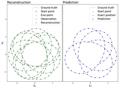
Figure 1: Learning measure-preserving flow map using measure-preserving neural networks.

Figure 1 demonstrates the ability of measure-preserving networks to fit and extrapolate measure-preserving map numerically. Here, the training data $\{(x_{n},x_{n+1})\}_{n=0}^{199}$ is obtained by sampling states on a single trajectory of a 4-dimensional divergence-free dynamical system. And we aim to approximate the flow map $\psi$ that maps $x_{n}$ to $x_{n+1}$ using measure-preserving network $\psi_{net}$. After training, we reconstruct the trajectory and perform predictions for $100$ steps starting at $x_{200}$. All trajectories are projected onto the first two dimensions. More experimental details are shown in A. It is observed that the measure-preserving model successfully reconstructs and predicts the evolution of the measure-preserving flow.

4.2 Application scopes of the approximation theory

The expected error of neural networks can be divided into three main types: approximation, optimization, and generalization (Bottou and Bousquet, 2007; Bottou, 2010; Jin et al., 2020a). See Figure 2 for the illustration.

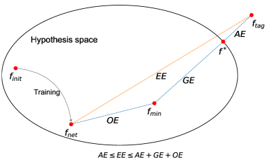
Figure 2: Illustration of optimization error (OE), generalization error (GE), approximation error (AE) and total expected error (EE). Here, $f_{net}$ is the network returned by the training algorithm starting at initial $f_{init}$. $f_{min}$ is the neural network which minimize empirical loss. $f_{tag}$ is the target ground-truth function, and $f^{*}$ is the network closest to $f_{tag}$ in the hypothesis space.

One of the key target in deep learning is to develop algorithms to increase accuracy, while the premise of this purpose is a good upper bound of approximation error. In addition, the approximation error is a crucial part of expected error. For structured deep neural networks, however, the approximation is different from the well-known universal approximation theory (Cybenko, 1989; Hornik et al., 1990) for fully connected networks obtained about 30 years ago and thus is attaching increasing attention (see Sec.1 3rd paragraph). Here, two application scenarios are important to discuss.

The first is that the target function is speculated to have a specific structure (e.g., CNN for image processing (Krizhevsky et al., 2012), measure-preserving modules in Poisson networks (Jin et al., 2020b)), or there exists prior knowledge exactly (e.g., HNN for discovery Hamiltonian systems (Greydanus et al., 2019), DeepONet for learning nonlinear operators (Lu et al., 2021a), measure-preserving networks for identifying divergence-free dynamics). The approximation theory in this paper indicates the approximation error can be made sufficiently small, which theoretically guarantees the feasibility of measure-preserving network modeling measure-preserving map and provides a key ingredient to the error analysis of learning algorithms using measure-preserving models.

The second is that the target function does not involve structures, but the employed network is designed for certain objectives, such as RevNets for avoiding storing intermediate activation (Gomez et al., 2017), generating models including NICE (Dinh et al., 2015) for computing inverse and Jacobian determinants efficiently, and measure-preserving networks for obtaining exact bijection of lossless compression (Zhang et al., 2021). This compromise of expressivity has a significant impact on performance (Dinh et al., 2017; Chen et al., 2018, 2019; Huang et al., 2018; Kingma and Dhariwal, 2018). And the approximation results mathematically characterize the limitation of the measure-preserving networks studied in this paper. In addition, our theory indicates that the approximation error mainly depends on the distance between the target function and measure-preserving function space. It would be an interesting future work to quantify this distance although it is not related to neural network theory. One possible approach is polar factorization (Brenier, 1991).

5 Proofs

Throughout this section we assume that $\Psi$ is defined as in (5) with control families $\mathcal{NN}^{d}$ ($d=D-s+1,s-1$) satisfied Assumption 1.

5.1 Properties of measure-preserving neural networks

Consider the following auxiliary measure-preserving modules of the form

$$R^{i}_{K,a,b}(x)=\begin{pmatrix}x[\ :i]\\ x[i]+\hat{\sigma}_{K,a,b}(\overline{x[i]})\\ x[i+1:\ ]\end{pmatrix}$$

with $1\leq i\leq D$. Here, $\hat{\sigma}_{K,a,b}$ specifies a fully connected neural network with one hidden layer, i.e.,

$$\hat{\sigma}_{K,a,b}(\overline{x[i]})=a\sigma(K\overline{x[i]}+b),\ K\in\mathbb{R}^{W\times(D-1)},b\in\mathbb{R}^{W\times 1},a\in\mathbb{R}^{1\times W},$$

where $\sigma:\mathbb{R}\rightarrow\mathbb{R}$ is the smooth activation function sigmoid $Sig(z)=1/(1+e^{-z})$ with Lipschitz constant $L_{\sigma}$. By the universal approximation theorem, $\hat{\sigma}_{K,a,b}$ can approximate any smooth function.

We denote the collection of $R^{i}_{K,a,b}$ as

$$\mathcal{R}^{i}=\{R^{i}_{K,a,b}|K\in\mathbb{R}^{W\times(D-1)},b\in\mathbb{R}^{W\times 1},a\in\mathbb{R}^{1\times W}\}.$$

Lemma 2 states that the auxiliary measure-preserving modules defined above can be approximated by measure-preserving neural networks. To prove this claim, we start with the following auxiliary lemma.

Lemma 1.

Given a sequence of $\varphi^{1},\cdots,\varphi^{N}$ which map from $\mathbb{R}^{D}$ to $\mathbb{R}^{D}$ and are Lipschitz on any compact set. If $\varphi^{k}\in\overline{\Psi}_{U}$ holds on any compact $U$, $1\leq k\leq N$, then $\varphi^{N}\circ\cdots\circ\varphi^{1}\in\overline{\Psi}_{U}$ holds on any compact $U$.

Proof.

We prove this lemma by induction. To begin with, the case $N=1$ is obvious. Suppose that this lemma holds when $N=n$. For the case $N=n+1$, given compact $U\in\mathbb{R}^{D}$, define

$$V=\bigcup_{k=1}^{n+1}\varphi^{k}\circ\cdots\circ\varphi^{1}(U)\cup U$$

and

$$E(V)=\{x\in\mathbb{R}^{D}\ |\ \exists x^{\prime}\in V\ \text{s.t.}\left\lVert x-x^{\prime}\right\rVert_{\infty}\leq 1\},$$

where $V$ and $E(V)$ are both compact. According to the induction hypothesis, we know that for any $0<\varepsilon<1$ there exists $\phi\in\Psi$ such that

$$\left\lVert\varphi^{n}\circ\cdots\circ\varphi^{1}-\phi\right\rVert_{U}\leq\varepsilon.$$

This inequality together with the condition $\varphi^{n}\circ\cdots\circ\varphi^{1}(U)\subset V$ yields that $\phi(U)\subset E(V)$. Since $\varphi^{n+1}\in\overline{\Psi}_{E(V)}$ we can choose $\phi^{\prime}\in\Psi$ such that

$$\left\lVert\varphi^{n+1}-\phi^{\prime}\right\rVert_{E(V)}\leq\varepsilon.$$

By the triangle inequality we have

$$\left\lVert\varphi^{n+1}\circ\cdots\circ\varphi^{1}-\phi^{\prime}\circ\phi\right\rVert_{U}$$

$$\leq \left\lVert\varphi^{n+1}\circ\cdots\circ\varphi^{1}-\varphi^{n+1}\circ\phi\right\rVert_{U}+\left\lVert\varphi^{n+1}\circ\phi-\phi^{\prime}\circ\phi\right\rVert_{U}$$

$$\leq L\left\lVert\varphi^{n}\circ\cdots\circ\varphi^{1}-\phi\right\rVert_{U}+\left\lVert\varphi^{n+1}-\phi^{\prime}\right\rVert_{E(V)}$$

$$\leq (L+1)\varepsilon,$$

where $L$ is the Lipschitz constant of $\varphi^{n+1}$ on $E(V)$. Note that $\phi^{\prime}\circ\phi\in\Psi$, hence

$$\varphi^{n+1}\circ\cdots\circ\varphi^{1}\in\overline{\Psi}_{U},$$

which completes the induction. ∎

Lemma 2.

$\mathcal{R}^{i}\subset\overline{\Psi}_{U}$ for any compact set $U\subset\mathbb{R}^{D}$, $1\leq i\leq D$.

Proof.

Without loss of generality, we assume $i=1$ and $u=R^{1}_{K,a,b}$. Taking

$$\phi^{w}(x)=\begin{pmatrix}x[1]+a[w]\sigma(K[w]x[2:\ ]+b[w])\\ x[2:\ ]\end{pmatrix}$$

for $w=1,\cdots,W$ yields

$$u=\phi^{W}\circ\cdots\circ\phi^{1}.$$

It is easy to verify that $\phi^{w}$ is Lipschitz on any compact set . In order to apply Lemma 1, it suffices to show $\phi^{w}\in\overline{\Psi}_{V}$ for $w=1,\cdots,W$ and any compact $V$, we will do it by construction.

Given any $\epsilon>0$, for $\delta>0$ satisfying $K[w][s-1]+\delta\neq 0$, define

$$\phi^{w1}(x) =\begin{pmatrix}x[\ :s]\\ x[s]+(K[w][s-1]+\delta)^{-1}K[w][\ :s-1]x[2:s]\\ x[s+1:\ ]\end{pmatrix},$$

$$\phi^{w2}(x) =\begin{pmatrix}\begin{aligned} x[1]+a[w]\sigma\Big{(}&(K[w][s-1]+\delta)x[s]\\ &+K[w][s:\ ]x[s+1:\ ]+b[w]\Big{)}\end{aligned}\\ x[2:\ ]\end{pmatrix},$$

$$\phi^{w3}(x) =\begin{pmatrix}x[\ :s]\\ x[s]-(K[w][s-1]+\delta)^{-1}K[w][\ :s-1]x[2:s]\\ x[s+1:\ ]\end{pmatrix}.$$

We could readily check that

$$\phi^{w3}\circ\phi^{w2}\circ\phi^{w1}=\begin{pmatrix}x[1]+a[w]\sigma(K[w]x[2:\ ]+b[w]+\delta x[s])\\ x[2:\ ]\end{pmatrix}.$$

Since

$$\left\lVert\phi^{w3}\circ\phi^{w2}\circ\phi^{w1}-\phi^{w}\right\rVert_{V}\leq C\delta$$

holds for a constant $C$, we can choose a small $\delta$ such that $C\delta<\frac{1}{2}\epsilon$. Furthermore, we have $\phi^{wi}\in\overline{(\mathcal{M}_{up}\cup\mathcal{M}_{low})}_{U^{\prime}}\subset\overline{\Psi}_{U^{\prime}}$ for any compact $U^{\prime}$ according to the second item of Assumpion 1. Applying Lemma 1 again and we have $\phi^{w3}\circ\phi^{w2}\circ\phi^{w1}\in\overline{\Psi}_{V}$, thus there exists $\psi\in\Psi$ such that

$$\left\lVert\psi-\phi^{w3}\circ\phi^{w2}\circ\phi^{w1}\right\rVert_{V}\leq\frac{1}{2}\epsilon.$$

Therefore

$$\left\lVert\psi-\phi^{w}\right\rVert_{V} \leq\left\lVert\psi-\phi^{w3}\circ\phi^{w2}\circ\phi^{w1}\right\rVert_{V}+\left\lVert\phi^{w3}\circ\phi^{w2}\circ\phi^{w1}-\phi^{w}\right\rVert_{V}$$

$$\leq\frac{1}{2}\epsilon+\frac{1}{2}\epsilon=\epsilon,$$

hence $\phi^{w}\in\overline{\Psi}_{V}$. ∎

The auxiliary modules are also measure-preserving but using special dimension-splitting mechanisms. Clearly, a element in $\mathcal{M}_{up}$ can be written as composition of $s-1$ maps like

$$R^{i}_{f_{net}}(x)=\begin{pmatrix}x[\ :i]\\ x[i]+f_{net}(\overline{x[i]})\\ x[i+1:\ ]\end{pmatrix}.$$

This fact together with Lemma 2 concludes that different choices of $s$ in control family lead to same approximation results theoretically, thus we use symbol $\Psi$ without emphasizing $s$.

In addition, we show that translation invariance of $\Psi$. This property will be used in Subsection 5.3.

Property 1.

Given $a\in\mathbb{R}^{D}$. If $\psi_{net}\in\Psi$, then $\psi_{net}+a\in\overline{\Psi}_{U}$ for any compact $U$.

Proof.

For any compact $U$, let

$$m^{1}: \hat{x}[\ :s]=x[\ :s]+a[\ :s],\ \hat{x}[s:\ ]=x[s:\ ];$$

$$m^{2}: \hat{x}[\ :s]=x[\ :s],\ \hat{x}[s:\ ]=x[s:\ ]+a[s:\ ].$$

We have $m^{i}\in\overline{(\mathcal{M}_{up}\cup\mathcal{M}_{low})}_{U^{\prime}}\subset\overline{\Psi}_{U^{\prime}},i=1,2$ for any compact $U^{\prime}$ according to the second item of Assumpion 1. By Lemma 1 we know

$$m^{2}\circ m^{1}\circ\psi_{net}\in\overline{\Psi}_{U},$$

which concludes the property. ∎

5.2 Approximation results for flow maps

Recently, the dynamical systems approach led to much progress in the theoretical underpinnings of deep learning (E, 2017; E et al., 2019; Li et al., 2017). In particular, Li et al. (2020) build approximation theory for continuous-time deep residual neural networks. These developments inspire us to apply differential equation techniques to complete the proof. The results of this work also serves the effectiveness of the dynamic system approach for understanding deep learning. Consider a differential equation

$$\frac{d}{dt}y(t)=f(t,y(t)),\quad y(\tau)=x,\tau\geq 0,$$ (6)

where $y(t)\in\mathbb{R}^{D}$, $f:[0,+\infty)\times\mathbb{R}^{D}\rightarrow\mathbb{R}^{D}$ is smooth. For a given time step $T\geq 0$, $y(\tau+T)$ could be regarded as a function of its initial condition $x$. We denote $\varphi_{\tau,T,f}(x):=y(\tau+T)$, which is known as the time-$T$ flow map of the dynamical system (6). We also write the collection of such flow maps as

$$\mathcal{F}(U)=\left\{\varphi_{\tau,T,f}:U\rightarrow\mathbb{R}^{D}\ \big{|}\ \tau,T\geq 0,\ f\in C^{\infty}([0,+\infty)\times\mathbb{R}^{D})\right\}.$$

Following (Hairer et al., 1993, 2006), we briefly recall some essential supporting results of numerical integrators here.

Definition 2.

Given system (6), an integrator $\Phi_{\tau,h,f}$ with time step $h$ has order $p$, if for compact $U\subset\mathbb{R}^{D}$, and any $\tau^{\prime}$ in a compact time interval, there exists constant $C$ such that for sufficiently small step $h>0$,

$$\left\lVert\Phi_{\tau^{\prime},h,f}-\varphi_{\tau^{\prime},h,f}\right\rVert_{U}\leq Ch^{p+1}.$$

The order of integrator is usually pointwise defined in the literature. Here $U$ is compact and thus the above definition accords with the literature. The simplest numerical integrator is the explicit Euler method,

$$\Phi_{\tau,h,f}^{e}(x)=x+hf(\tau,x).$$

Another scheme will be used in this paper is a splitting method. For system (6), if $f=\sum_{k=1}^{K}f^{k}$, the formula is given as

$$\Phi_{\tau,h,f}^{s}(x)=\varphi_{\tau,h,f^{K}}\circ\cdots\circ\varphi_{\tau,h,f^{1}}(x).$$

The above numerical integrators are both of order $1$.

Next, we turn to the approximation aspects of measure-preserving flow maps. Measure-preserving is a certain geometric structure of continuous dynamical systems. As demonstrated in (Hairer et al., 2006, Section VI.6), measure is preserved by the flow of differential equations with a divergence-free vector field.

Proposition 1.

The flow map of system (6) is measure-preserving if and only if

$$\operatorname{div}_{y}f=\sum_{d=1}^{D}\frac{\partial f_{d}}{\partial y_{d}}=0,$$

where $f=(f_{1},\cdots,f_{D})^{\top}$, $y=(y_{1},\cdots,y_{D})^{\top}$.

By Proposition 1, we denote the set of measure-preserving flow maps as

$$\mathcal{VF}(U)=\left\{\varphi_{\tau,T,f}\in\mathcal{F}(U)\ \big{|}\ \operatorname{div}_{y}f=0\right\}.$$

Subsequently, we introduce two kinds of vector fields of measure-preserving flow maps.

Definition 3.

For $f:[0,+\infty)\times\mathbb{R}^{D}\rightarrow\mathbb{R}^{D}$ and $1\leq d\leq D-1$, we say $f$ is $2$-Hamiltonian in the $d,d+1$-th variables if there exists a scalar function $H:[0,+\infty)\times\mathbb{R}^{D}\rightarrow\mathbb{R}$ such that

$$f=(\underbrace{0,\cdots,0}_{d-1},-\frac{\partial H}{\partial y_{d+1}},\frac{\partial H}{\partial y_{d}},\underbrace{0,\cdots,0}_{D-d-1})^{\top}.$$

Definition 4.

For $f:[0,+\infty)\times\mathbb{R}^{D}\rightarrow\mathbb{R}^{D}$ and $1\leq d\leq D-1$, we say $f$ is separable $2$-Hamiltonian in the $d,d+1$-th variables if there exist two scalar functions $g_{1},g_{2}:[0,+\infty)\times\mathbb{R}^{D-1}\rightarrow\mathbb{R}$ such that

$$f=(\underbrace{0,\cdots,0}_{d-1},g_{1}(t,\overline{y[d]}),g_{2}(t,\overline{y[d+1]}),\underbrace{0,\cdots,0}_{D-d-1})^{\top}.$$

Clearly, a separable $2$-Hamiltonian $f$ is $2$-Hamiltonian and both are divergence-free. Below we will establish the approximation results for flow maps with separable 2-Hamiltonian vector fields (Lemma 4) and 2-Hamiltonian vector fields (Lemma 5), and finally obtain the approximation theory of measure-preserving flow maps (Lemma 6).

To this end, we present the composition approximation for flow map firstly, which will be used frequently.

Lemma 3.

Given smooth $f:[0,+\infty)\times\mathbb{R}^{D}\rightarrow\mathbb{R}^{D}$ and $\varphi_{\tau,T,f}\in\mathcal{F}(U)$ with compact set $U\subset\mathbb{R}^{D}$. If on any compact $U^{\prime}$, there exists $\phi\in\Psi$ such that

$$\left\lVert\varphi_{\tau^{\prime},h,f}-\phi\right\rVert_{U^{\prime}}\leq Ch^{2}$$

holds for any $\tau^{\prime}\in[\tau,\tau+T]$ and any sufficiently small step $h>0$, then,

$$\varphi_{\tau,T,f}\in\overline{\Psi}_{U}.$$

Proof.

Define

$$V=\{\varphi_{\tau^{\prime},T^{\prime},f}(x)\ |\ x\in U,\ \tau\leq\tau^{\prime}\leq\tau^{\prime}+T^{\prime}\leq\tau+T\},$$

and for $i=1,2$,

$$E^{i}(V)=\{x\in\mathbb{R}^{D}\ |\ \exists x^{\prime}\in V\ \text{s.t.}\left\lVert x-x^{\prime}\right\rVert_{\infty}\leq i\},$$

where $V$ and $E^{i}(V)$ are compact since $f$ is smooth. Let

$$L=1+\sup\limits_{\begin{subarray}{c}\tau\leq\tau^{\prime}\leq\tau^{\prime}+T^{\prime}\leq\tau+T\\ x\in{E^{2}(V)}\end{subarray}}\left\lVert\frac{\partial\varphi_{\tau^{\prime},T^{\prime},f}(x)}{\partial x}\right\rVert_{\infty}.$$

And for any $0<\varepsilon<1$, take

$$N>\frac{1}{\varepsilon}(LCT^{2}+T\left\lVert f\right\rVert_{[\tau,\tau+T]\times E^{2}(V)}),\quad h=\frac{T}{N}.$$

Then there exists a sequence of $\phi_{N-1},\cdots,\phi_{0}\in\Psi$, such that, for $0\leq k\leq N-1$,

$$\left\lVert\varphi_{\tau+kh,h,f}-\phi_{k}\right\rVert_{E^{1}(V)}\leq Ch^{2}.$$

To conclude the lemma, it suffices to show that

$$\left\lVert\varphi_{\tau,nh,f}-\phi_{n-1}\circ\cdots\circ\phi_{0}\right\rVert_{U}\leq n\cdot L\cdot C\cdot\frac{T^{2}}{N^{2}}$$

for any $1\leq n\leq N$. We now prove this statement by induction on $1\leq n\leq N$. First, the case when $n=1$ is obvious. Suppose now

$$\left\lVert\varphi_{\tau,kh,f}-\phi_{k-1}\circ\cdots\circ\phi_{0}\right\rVert_{U}\leq k\cdot L\cdot C\cdot\frac{T^{2}}{N^{2}}$$

for $k\leq n-1$. This inductive hypothesis implies $\phi_{k-1}\circ\cdots\circ\phi_{0}(U)\subset E^{1}(V)$ and thus

$$\phi_{k}\circ\phi_{k-1}\circ\cdots\circ\phi_{0}(U)\subset E^{2}(V),$$

$$\varphi_{\tau+kh,h,f}\circ\phi_{k-1}\circ\cdots\circ\phi_{0}(U)\subset E^{2}(V),$$

where we have used the fact that for any $x\in E^{1}(V)$,

$$\left\lVert\varphi_{\tau+kh,h,f}(x)-x\right\rVert_{\infty} =\left\lVert\int_{\tau+kh}^{\tau+(k+1)h}f(t,x(t))dt\right\rVert_{\infty}$$

$$\leq h\left\lVert f\right\rVert_{[\tau,\tau+T]\times E^{2}(V)}\leq\varepsilon<1,$$

and

$$\left\lVert\phi_{k}(x)-x\right\rVert_{\infty} \leq\left\lVert\varphi_{\tau+kh,h,f}(x)-x\right\rVert_{\infty}+Ch^{2}$$

$$\leq h\left\lVert f\right\rVert_{[\tau,\tau+T]\times E^{2}(V)}+Ch^{2}\leq\varepsilon<1.$$

Subsequently, denote $L_{k}=\sup_{x\in E^{2}(V)}\left\lVert\frac{\partial\varphi_{\tau+(k+1)h,(n-k-1)h,f}(x)}{\partial x}\right\rVert_{\infty}\leq L$, we obtain

$$\left\lVert\varphi_{\tau,nh,f}-\phi_{n-1}\circ\cdots\circ\phi_{0}\right\rVert_{U}$$

$$\leq \Big{(}\sum_{k=1}^{n-1}\|\varphi_{\tau+kh,(n-k)h,f}\circ\phi_{k-1}\circ\cdots\circ\phi_{0}$$

$$\quad-\varphi_{\tau+(k+1)h,(n-k-1)h,f}\circ\phi_{k}\circ\cdots\circ\phi_{0}\|_{U}\Big{)}$$

$$+\left\lVert\varphi_{\tau,nh,f}-\varphi_{\tau+h,(n-1)h,f}\circ\phi_{0}\right\rVert_{U}$$

$$\leq \sum_{k=1}^{n-1}L_{k}\left\lVert\varphi_{\tau+kh,h,f}\circ\phi_{k-1}\circ\cdots\circ\phi_{0}-\phi_{k}\circ\cdots\circ\phi_{0}\right\rVert_{U}$$

$$+L_{0}\left\lVert\varphi_{\tau,h,f}-\phi_{0}\right\rVert_{U}$$

$$\leq \sum_{k=1}^{n-1}L\left\lVert\varphi_{\tau+kh,h,f}-\phi_{k}\right\rVert_{E^{1}(V)}+LC\frac{T^{2}}{N^{2}}$$

$$\leq n\cdot L\cdot C\cdot\frac{T^{2}}{N^{2}}.$$

Hence the induction holds and the proof is completed. ∎

Lemma 4.

Given compact $U\subset\mathbb{R}^{D}$ and $\varphi_{\tau,T,f}\in\mathcal{F}(U)$. If the vector fields $f$ is separable $2$-Hamiltonian in the $d,d+1$-th variables with $1\leq d\leq D-1$, then,

$$\varphi_{\tau,T,f}\in\overline{\Psi}_{U}.$$

Proof.

Without loss of generality, we assume $d=1$. The relation between $x$ and $\varphi_{\tau,T,f}(x)$ is characterized by the following equation,

$$\frac{d}{dt}y(t)=f(t,y(t)),\quad y(\tau)=x,\ y(\tau+T)=\varphi_{\tau,T,f}(x).$$ (7)

For $y=(y_{1},y_{2},y_{3},\cdots,y_{d})$, denote $p=y_{1},q=y_{2},\mu=(y_{3},\cdots,y_{d})^{\top}$. Since $f$ is separable $2$-Hamiltonian in the $1,2$-th variables, there exist two scalar functions $g_{1},g_{2}:[0,+\infty)\times\mathbb{R}^{D-1}\rightarrow\mathbb{R}$ such that equation (7) can be written as

$$\frac{d}{dt}p(t) =g_{1}(t,q,\mu),$$ (8)

$$\frac{d}{dt}q(t) =g_{2}(t,p,\mu),$$

$$\frac{d}{dt}\mu(t) =0.$$

For any $\tau^{\prime}\in[\tau,\tau+T]$ and any sufficiently small step $h>0$, define the following map

$$\phi_{\tau^{\prime},h}^{1}(p,q,\mu) =(p+hg_{1}(\tau^{\prime},q,\mu),q,\mu^{\top})^{\top},$$

$$\phi_{\tau^{\prime},h}^{2}(p,q,\mu) =(p,q+hg_{2}(\tau^{\prime},p,\mu),\mu^{\top})^{\top},$$

$$\phi_{\tau^{\prime},h} =\phi_{\tau^{\prime},h}^{2}\circ\phi_{\tau^{\prime},h}^{1}.$$

Here, $\phi_{\tau^{\prime},h}$ is the splitting integrator applied to system (8), which is an integrator of order one. Therefore, for any compact $U^{\prime}$, there exists constant $C$ such that

$$\left\lVert\varphi_{\tau^{\prime},h,f}-\phi_{\tau^{\prime},h}\right\rVert_{U^{\prime}}\leq Ch^{2}.$$

In addition, for any compact $V$, the universal approximation theorem of neural networks with one hidden layer and sigmoid activation together with Lemma 2 implies

$$\phi_{\tau^{\prime},h}^{1}\in\overline{\mathcal{R}^{1}}_{V}\subset\overline{\Psi}_{V},$$

$$\phi_{\tau^{\prime},h}^{2}\in\overline{\mathcal{R}^{2}}_{V}\subset\overline{\Psi}_{V}.$$

By Lemma 1, we obtain $\phi_{\tau^{\prime},h}\in\overline{\Psi}_{U^{\prime}}$ and thus there exists $v\in\Psi$ such that

$$\left\lVert v-\phi_{\tau^{\prime},h}\right\rVert_{U^{\prime}}\leq h^{2}.$$

Finally, we conclude that

$$\left\lVert\varphi_{\tau^{\prime},h,f}-v\right\rVert_{U^{\prime}}\leq(C+1)h^{2},$$

and the lemma is completed by applying Lemma 3. ∎

Proposition 2.

Given any non-autonomous $H(t,p,q,\mu)$ with bounded parameter $\mu$, polynomial in $p,q\in\mathbb{R}$, and the Hamiltonian system

$$\frac{d}{dt}p(t)=-\frac{\partial H}{\partial q}(t,p,q,\mu),$$

$$\frac{d}{dt}q(t)=\frac{\partial H}{\partial p}(t,p,q,\mu).$$

Denote $f_{1}=(-\frac{\partial H}{\partial q},\frac{\partial H}{\partial p})^{\top}$. Then on any compact domain $U$ in the $(p,q,\mu)$-space and any compact interval of the values of $\tau$, there exists a scalar function $V(t,q,\mu)$ polynomial in $q$, such that, for any sufficiently small step $h>0$, the time-$2\pi$ flow map of the Hamiltonian system

$$\frac{d}{dt}p(t)=-q-h\cdot\frac{\partial V}{\partial q}(t,q,\mu),$$

$$\frac{d}{dt}q(t)=p,$$

denoted as $\varphi_{0,2\pi,f_{2}}$ with $f_{2}=(-q-h\frac{\partial V}{\partial q}(t,q,\mu),p)^{\top}$, satisfies

$$\sup_{(p,q,\mu)\in U}\left\lVert\varphi_{0,2\pi,f_{2}}(p,q)-\varphi_{\tau,h,f_{1}}(p,q)\right\rVert_{\infty}\leq Ch^{2}$$

with constant $C$.

Proof.

The proposition is the 2-dimensional case of (Turaev, 2002, Lemma 1). ∎

With Proposition 2, we can approximate the flow maps with 2-Hamiltonian vector fields, which give rise to the following lemma.

Lemma 5.

Given compact $U\subset\mathbb{R}^{D}$ and $\varphi_{\tau,T,f}\in\mathcal{F}(U)$. If the vector fields $f$ is $2$-Hamiltonian in the $d,d+1$-th variables with $1\leq d\leq D-1$, then,

$$\varphi_{\tau,T,f}\in\overline{\Psi}_{U}.$$

Proof.

Without loss of generality, we assume $d=1$. The relation between $x$ and $\varphi_{\tau,T,f}(x)$ is characterized by the following equation,

$$\frac{d}{dt}y(t)=f(t,y(t)),\quad y(\tau)=x,\ y(\tau+T)=\varphi_{\tau,T,f}(x).$$ (9)

For $y=(y_{1},y_{2},y_{3},\cdots,y_{d})$, denote $p=y_{1},q=y_{2},\mu=(y_{3},\cdots,y_{d})^{\top}$. Since $f$ is $2$-Hamiltonian in the $1,2$-th variables, there exists a scalar function $H:[0,+\infty)\times\mathbb{R}^{D}\rightarrow\mathbb{R}$ such that equation (9) can be written as

$$\frac{d}{dt}p(t) =-\frac{\partial H}{\partial q}(t,p,q,\mu),$$

$$\frac{d}{dt}q(t) =\frac{\partial H}{\partial p}(t,p,q,\mu),$$

$$\frac{d}{dt}\mu(t) =0.$$

On any compact $U^{\prime}$, since polynomials are dense among smooth functions, for any sufficiently small step $h>0$, there exists $H_{poly}$, polynomial in $p,q$, such that

$$\left\lVert\frac{\partial H}{\partial q}-\frac{\partial H_{ploy}}{\partial q}\right\rVert_{[\tau,\tau+T]\times U^{\prime}}+\left\lVert\frac{\partial H}{\partial p}-\frac{\partial H_{ploy}}{\partial p}\right\rVert_{[\tau,\tau+T]\times U^{\prime}}\leq h.$$

Consider the Hamiltonian system with Hamiltonian $H_{ploy}$, i.e.,

$$\frac{d}{dt}p(t) =-\frac{\partial H_{ploy}}{\partial q}(t,p,q,\mu),$$ (10)

$$\frac{d}{dt}q(t) =\frac{\partial H_{ploy}}{\partial p}(t,p,q,\mu),$$

$$\frac{d}{dt}\mu(t) =0.$$

Denote $f_{1}=(-\frac{\partial H_{ploy}}{\partial q},\frac{\partial H_{ploy}}{\partial p},0)^{\top}$, for $\tau^{\prime}\in[\tau,\tau+T]$, the time-$h$ flow map of (10) starting at $\tau^{\prime}$ can be written as $\varphi_{\tau^{\prime},h,f_{1}}$. Due to the difference between $f$ and $f_{1}$, there is a constant $C_{1}$ such that

$$\left\lVert\varphi_{\tau^{\prime},h,f_{1}}-\varphi_{\tau^{\prime},h,f}\right\rVert_{U^{\prime}}$$

$$\leq \left\lVert\varphi_{\tau^{\prime},h,f_{1}}-\Phi_{\tau^{\prime},h,f_{1}}^{e}\right\rVert_{U^{\prime}}+\left\lVert\Phi_{\tau^{\prime},h,f_{1}}^{e}-\Phi_{\tau^{\prime},h,f}^{e}\right\rVert_{U^{\prime}}+\left\lVert\Phi_{\tau^{\prime},h,f}^{e}-\varphi_{\tau^{\prime},h,f}\right\rVert_{U^{\prime}}$$

$$\leq C_{1}h^{2}.$$

According to Proposition 2, there exists a function $V(t,q,\mu)$ polynomial in $q$ and a Hamiltonian system of the form

$$\frac{d}{dt}p(t) =-q-h\cdot\frac{\partial V}{\partial q}(t,q,\mu),$$ (11)

$$\frac{d}{dt}q(t) =p,$$

$$\frac{d}{dt}\mu(t) =0,$$

such that, the time-$2\pi$ map of (11), denoted as $\varphi_{0,2\pi,f_{2}}$ with $f_{2}=(-q-h\frac{\partial V}{\partial q}(t,q,\mu),p,0)^{\top}$, satisfies

$$\left\lVert\varphi_{0,2\pi,f_{2}}-\varphi_{\tau^{\prime},h,f_{1}}\right\rVert_{U^{\prime}}\leq C_{2}h^{2}$$

with constant $C_{2}$. Hence,

$$\left\lVert\varphi_{0,2\pi,f_{2}}-\varphi_{\tau^{\prime},h,f}\right\rVert_{U^{\prime}} \leq\left\lVert\varphi_{0,2\pi,f_{2}}-\varphi_{\tau^{\prime},h,f_{1}}\right\rVert_{U^{\prime}}+\left\lVert\varphi_{\tau^{\prime},h,f_{1}}-\varphi_{\tau^{\prime},h,f}\right\rVert_{U^{\prime}}$$

$$\leq(C_{1}+C_{2})h^{2}.$$

Subsequently, by Lemma 4, there exists $v\in\Psi$ such that

$$\left\lVert v-\varphi_{\tau^{\prime},h,f}\right\rVert_{U^{\prime}} \leq\left\lVert\varphi_{0,2\pi,f_{2}}-v\right\rVert_{U^{\prime}}+\left\lVert\varphi_{\tau^{\prime},h,f_{2}}-\varphi_{\tau^{\prime},h,f}\right\rVert_{U^{\prime}}$$

$$\leq(C_{1}+C_{2}+1)h^{2}.$$

The lemma is completed as a consequence of Lemma 3. ∎

Proposition 3.

If $f:[0,+\infty)\times\mathbb{R}^{D}\rightarrow\mathbb{R}^{D}$ obeys $\operatorname{div}f=0$, then $f$ can be written as the sum of $D-1$ vector fields

$$f=f_{1,2}+f_{2,3}+\cdots+f_{D-1,D},$$

where each $f_{d,d+1}$ is $2$-Hamiltonian in the $d,d+1$-th variables for $1\leq d\leq D-1$. Furthermore, if $f$ is smooth, $f_{d,d+1}$ is smooth.

Proof.

The proof can be found in (Feng and Shang, 1995). ∎

Proposition 3 is founded by Feng and Shang to develop integrator for divergence-free equations. With the decomposition of Proposition 3, the gap between divergence-free and 2-Hamiltonian vector fields is bridged.

Lemma 6.

Given compact $U\subset\mathbb{R}^{D}$ and $\varphi_{\tau,T,f}\in\mathcal{VF}(U)$, then,

$$\varphi_{\tau,T,f}\in\overline{\Psi}_{U}.$$

Viz., $\mathcal{VF}(U)\subset\overline{\Psi}_{U}$.

Proof.

By Proposition 3, $f$ can be written as the sum of $D-1$ vector fields

$$f=f_{1,2}+f_{2,3}+\cdots+f_{D-1,D},$$

where each $f_{d,d+1}$ is $2$-Hamiltonian in the $d,d+1$-th variables. For any compact set $U^{\prime}\subset\mathbb{R}^{D}$, any $\tau^{\prime}\in[\tau,\tau+T]$ and any sufficiently small step $h>0$, taking the splitting integrator

$$\phi_{\tau^{\prime},h}=\varphi_{\tau^{\prime},h,f_{D-1,D}}\circ\cdots\circ\varphi_{\tau^{\prime},h,f_{1,2}}$$

implies

$$\left\lVert\varphi_{\tau^{\prime},h,f}-\phi_{\tau^{\prime},h}\right\rVert_{U^{\prime}}\leq Ch^{2}.$$

In addition, for any compact $V$, due to Lemma 5, we have

$$\varphi_{\tau^{\prime},h,f_{d,d+1}}\in\overline{\Psi}_{V},$$

which implies $\phi_{\tau^{\prime},h}\in\overline{\Psi}_{U^{\prime}}$ according to Lemma 1. Therefore there exists $v\in\Psi$ such that

$$\left\lVert\varphi_{\tau^{\prime},h,f}-v\right\rVert_{U^{\prime}}\leq\left\lVert v-\phi_{\tau^{\prime},h}\right\rVert_{U^{\prime}}+\left\lVert\varphi_{\tau^{\prime},h,f}-\phi_{\tau^{\prime},h}\right\rVert_{U^{\prime}}\leq(C+1)h^{2}.$$

By Lemma 3, we obtain

$$\varphi_{\tau,T,f}\in\overline{\Psi}_{U},$$

which concludes the proof. ∎

5.3 Proof of Theorem 1

Proposition 4.

Suppose that $Q\in\mathbb{R}^{D}$ is an open cube and that $1\leq p<+\infty$. For every measure-preserving map $\psi:\overline{Q}\rightarrow\overline{Q}$ and arbitrary $\varepsilon>0$, there exists a time-$1$ flow map $\varphi_{0,1,f}\in\mathcal{VF}(Q)$ where $f$ is compactly supported in $(0,1)\times Q$ such that

$$\left\lVert\psi-\varphi_{0,1,f}\right\rVert_{L^{p}(Q)}\leq\varepsilon.$$

Proof.

The proof can be found in (Brenier and Gangbo, 2003, Corollary 1.1). ∎

With these results, we are able to provide the proof of the main theorems.

Proof of Theorem 1.

For compact $U\subset\mathbb{R}^{D}$, we can take $a\in\mathbb{R}^{D}$ satisfying $U\cap(\psi(U)+a)=\varnothing$. Let $Q$ be a open cube large enough such that $U,\psi(U)+a\subset Q$, and define $\tilde{\psi}$ on $Q$ by

$$\tilde{\psi}(x)=\left\{\begin{aligned} &\psi(x)+a,\quad&&\text{if }x\in U,\\ &\psi^{-1}(x-a),&&\text{if }x\in\psi(U)+a,\\ &x,\quad&&\text{if }x\in Q\setminus(U\cup(\psi(U)+a)).\end{aligned}\right.$$

Here, $\tilde{\psi}:Q\rightarrow Q$ is measure-preserving. According to Proposition 4 there exists a time-$1$ flow map $\varphi_{0,1,f}\in\mathcal{VF}(Q)$ such that

$$\left\lVert\tilde{\psi}-\varphi_{0,1,f}\right\rVert_{L^{p}(Q)}\leq\varepsilon,$$

and $f$ is compactly supported in $(0,1)\times Q$. Using Lemma 6 we deduce that there exists a measure-preserving neural network $\psi_{net}\in\Psi$ such that

$$\left\lVert\varphi_{0,1,f}-\psi_{net}\right\rVert_{L^{p}(Q)}\leq\varepsilon.$$

By these estimations, we obtain

$$\left\lVert\psi_{net}-\tilde{\psi}\right\rVert_{L^{p}(U)}=\left\lVert\psi_{net}-a-\psi\right\rVert_{L^{p}(U)}\leq 2\varepsilon,$$

and thus $\psi\in\overline{\Psi}_{L^{p}(U)}$ since $\psi_{net}-a\in\overline{\Psi}_{U}$. Hence, the theorem has been completed. ∎

6 Summary

The main contribution of this paper is to prove the approximation capabilities of measure-preserving neural networks. These results serve the mathematical foundations of existing measure-preserving neural networks such as NICE (Dinh et al., 2015) and RevNets (Gomez et al., 2017).

The key idea is introducing flow maps from the perspective of dynamical systems. Via investigation of approximation aspects of two special measure-preserving maps, i.e, flow maps of 2-Hamiltonian and separable 2-Hamiltonian vector fields, we show that every measure-preserving map can be approximated in $C$-norm by measure-preserving neural networks. Finally, by the $L^{p}$-norm approximation proposition which connects measure-preserving flow maps and general measure-preserving maps, we conclude the main theorem.

One open question is the $C$-norm approximation of Corollary 1. This issue is essentially the gap between measure-preserving flow map and general measure-preserving map. We conjecture that Proposition 4 can be further improved to provide $C$-norm approximation under additional assumptions of measure-preserving map. This paper also shows the effectiveness of understanding deep learning via dynamical systems. Exploring approximation aspects of other structured neural networks via flow map might be another interesting direction.

Appendix A Experimental details

We consider a divergence-free dynamical system given as

$$\dot{y}_{1} =y_{3},$$

$$\dot{y}_{2} =y_{4},$$

$$\dot{y}_{3} =\frac{y_{1}}{100(y_{1}^{2}+y_{2}^{2})^{\frac{3}{2}}}+(y_{1}^{2}+y_{2}^{2})^{\frac{1}{2}}y_{4},$$

$$\dot{y}_{4} =\frac{x_{2}}{100(y_{1}^{2}+y_{2}^{2})^{\frac{3}{2}}}-(y_{1}^{2}+y_{2}^{2})^{\frac{1}{2}}y_{3}.$$

This equation describes dynamics of a single charged particle in an electromagnetic field governed by Lorentz force. We can readily check that the governing function is divergence-free and thus its flow map is measure-preserving due to Proposition 1. The architecture used is a stack of 8 coupling layers with partition $s=2$, where single hidden layer neural network with width of $64$ and sigmoid activation is adopted as control families. We optimize the mean-squared-error loss

$$\frac{1}{I}\sum_{n=1}^{N}\|\psi_{net}(x_{n})-x_{n+1}\|^{2}$$

for $8\times 10^{5}$ epochs with Adam optimization and learning rate $0.001$. Here, $\{(x_{n},x_{n+1})\}_{n=0}^{N}$ is the training data with $N=199$ and is sampled on the trajectory starting at $(0.1,1,1.1,0.5)$ from $t=0$ to $t=40$ using equidistant time step size of $0.2$.

References

- Behrmann et al. (2019) Behrmann, J., Grathwohl, W., Chen, R.T.Q., Duvenaud, D., Jacobsen, J.H., 2019. Invertible residual networks, in: Proceedings of the 36th International Conference on Machine Learning, PMLR, Long Beach, California, USA. pp. 573–582.
- Bottou (2010) Bottou, L., 2010. Large-scale machine learning with stochastic gradient descent, in: Proceedings of COMPSTAT’2010, Physica-Verlag HD, Heidelberg. pp. 177–186.
- Bottou and Bousquet (2007) Bottou, L., Bousquet, O., 2007. The tradeoffs of large scale learning, in: Advances in Neural Information Processing Systems 20, Proceedings of the Twenty-First Annual Conference on Neural Information Processing Systems, Vancouver, British Columbia, Canada, December 3-6, 2007, Curran Associates, Inc.. pp. 161–168.
- Brenier (1991) Brenier, Y., 1991. Polar factorization and monotone rearrangement of vector-valued functions. Communications on pure and applied mathematics 44, 375–417.
- Brenier and Gangbo (2003) Brenier, Y., Gangbo, W., 2003. approximation of maps by diffeomorphisms. Calculus of Variations and Partial Differential Equations 16, 147–164.
- Chen and Tao (2021) Chen, R., Tao, M., 2021. Data-driven prediction of general hamiltonian dynamics via learning exactly-symplectic maps, in: Proceedings of the 38th International Conference on Machine Learning, ICML 2021, PMLR. pp. 1717–1727.
- Chen et al. (2019) Chen, T.Q., Behrmann, J., Duvenaud, D., Jacobsen, J., 2019. Residual flows for invertible generative modeling, in: Advances in Neural Information Processing Systems, pp. 9913–9923.
- Chen et al. (2018) Chen, T.Q., Rubanova, Y., Bettencourt, J., Duvenaud, D., 2018. Neural ordinary differential equations, in: Advances in Neural Information Processing Systems 31: Annual Conference on Neural Information Processing Systems 2018, NeurIPS 2018, December 3-8, 2018, Montréal, Canada, pp. 6572–6583.
- Cybenko (1989) Cybenko, G., 1989. Approximation by superpositions of a sigmoidal function. Mathematics of control, signals and systems 2, 303–314.
- Dinh et al. (2015) Dinh, L., Krueger, D., Bengio, Y., 2015. NICE: non-linear independent components estimation, in: 3rd International Conference on Learning Representations, ICLR 2015, San Diego, CA, USA, May 7-9, 2015, Workshop Track Proceedings.
- Dinh et al. (2017) Dinh, L., Sohl-Dickstein, J., Bengio, S., 2017. Density estimation using real NVP, in: 5th International Conference on Learning Representations, ICLR 2017, Toulon, France, April 24-26, 2017, Conference Track Proceedings, OpenReview.net.
- Dupont et al. (2019) Dupont, E., Doucet, A., Teh, Y.W., 2019. Augmented neural odes, in: Advances in Neural Information Processing Systems 32: Annual Conference on Neural Information Processing Systems 2019, NeurIPS 2019, December 8-14, 2019, Vancouver, BC, Canada, pp. 3134–3144.
- E (2017) E, W., 2017. A proposal on machine learning via dynamical systems. Communications in Mathematics and Statistics 5, 1–11.
- E et al. (2019) E, W., Han, J., Li, Q., 2019. A mean-field optimal control formulation of deep learning. Research in the Mathematical Sciences 6, 1–41.
- Feng and Shang (1995) Feng, K., Shang, Z., 1995. Volume-preserving algorithms for source-free dynamical systems. Numerische Mathematik 71, 451–463.
- Fiori (2011a) Fiori, S., 2011a. Extended Hamiltonian learning on Riemannian manifolds: Numerical aspects. IEEE Transactions on Neural Networks and Learning Systems 23, 7–21.
- Fiori (2011b) Fiori, S., 2011b. Extended Hamiltonian learning on Riemannian manifolds: Theoretical aspects. IEEE transactions on neural networks 22, 687–700.
- Gomez et al. (2017) Gomez, A.N., Ren, M., Urtasun, R., Grosse, R.B., 2017. The reversible residual network: Backpropagation without storing activations, in: Advances in Neural Information Processing Systems 30: Annual Conference on Neural Information Processing Systems 2017, 4-9 December 2017, Long Beach, CA, USA, pp. 2214–2224.
- Greydanus et al. (2019) Greydanus, S., Dzamba, M., Yosinski, J., 2019. Hamiltonian neural networks, in: Advances in Neural Information Processing Systems 32: Annual Conference on Neural Information Processing Systems 2019, NeurIPS 2019, December 8-14, 2019, Vancouver, BC, Canada, pp. 15353–15363.
- Hairer et al. (2006) Hairer, E., Lubich, C., Wanner, G., 2006. Geometric numerical integration: structure-preserving algorithms for ordinary differential equations. volume 31. Springer Science & Business Media.
- Hairer et al. (1993) Hairer, E., Norsett, S., Wanner, G., 1993. Solving Ordinary Differential Equations I: Nonstiff Problems. volume 8. Springer-Verlag, Berlin.
- He et al. (2016) He, K., Zhang, X., Ren, S., Sun, J., 2016. Deep residual learning for image recognition, in: 2016 IEEE Conference on Computer Vision and Pattern Recognition, CVPR 2016, Las Vegas, NV, USA, June 27-30, 2016, IEEE Computer Society. pp. 770–778.
- Hornik et al. (1990) Hornik, K., Stinchcombe, M., White, H., 1990. Universal approximation of an unknown mapping and its derivatives using multilayer feedforward networks. Neural Networks 3, 551 – 560.
- Huang et al. (2018) Huang, C., Krueger, D., Lacoste, A., Courville, A.C., 2018. Neural autoregressive flows, in: Proceedings of the 35th International Conference on Machine Learning, ICML 2018, Stockholmsmässan, Stockholm, Sweden, July 10-15, 2018, PMLR. pp. 2083–2092.
- Jin et al. (2020a) Jin, P., Lu, L., Tang, Y., Karniadakis, G.E., 2020a. Quantifying the generalization error in deep learning in terms of data distribution and neural network smoothness. Neural Networks 130, 85–99.
- Jin et al. (2020b) Jin, P., Zhang, Z., Kevrekidis, I.G., Karniadakis, G.E., 2020b. Learning poisson systems and trajectories of autonomous systems via poisson neural networks. arXiv preprint arXiv:2012.03133 .
- Jin et al. (2020c) Jin, P., Zhang, Z., Zhu, A., Tang, Y., Karniadakis, G.E., 2020c. Sympnets: Intrinsic structure-preserving symplectic networks for identifying hamiltonian systems. Neural Networks 132, 166 – 179.
- Kingma and Dhariwal (2018) Kingma, D.P., Dhariwal, P., 2018. Glow: Generative flow with invertible 1x1 convolutions, in: Advances in Neural Information Processing Systems 31: Annual Conference on Neural Information Processing Systems 2018, NeurIPS 2018, December 3-8, 2018, Montréal, Canada, pp. 10236–10245.
- Kong and Chaudhuri (2020) Kong, Z., Chaudhuri, K., 2020. The expressive power of a class of normalizing flow models, in: The 23rd International Conference on Artificial Intelligence and Statistics, AISTATS 2020, 26-28 August 2020, Online [Palermo, Sicily, Italy], PMLR. pp. 3599–3609.
- Krizhevsky et al. (2012) Krizhevsky, A., Sutskever, I., Hinton, G.E., 2012. Imagenet classification with deep convolutional neural networks, in: Advances in Neural Information Processing Systems 25, December 3-6, 2012, Lake Tahoe, Nevada, United States, pp. 1106–1114.
- Krizhevsky et al. (2017) Krizhevsky, A., Sutskever, I., Hinton, G.E., 2017. Imagenet classification with deep convolutional neural networks. Commun. ACM 60, 84–90.
- LeCun et al. (2015) LeCun, Y., Bengio, Y., Hinton, G.E., 2015. Deep learning. Nature 521, 436–444.
- Li et al. (2017) Li, Q., Chen, L., Tai, C., Weinan, E., 2017. Maximum principle based algorithms for deep learning. The Journal of Machine Learning Research 18, 5998–6026.
- Li et al. (2020) Li, Q., Lin, T., Shen, Z., 2020. Deep learning via dynamical systems: An approximation perspective. arXiv preprint arXiv:1912.10382 .
- Lu et al. (2021a) Lu, L., Jin, P., Pang, G., Zhang, Z., Karniadakis, G.E., 2021a. Learning nonlinear operators via deeponet based on the universal approximation theorem of operators. Nature Machine Intelligence 3, 218–229.
- Lu et al. (2021b) Lu, L., Meng, X., Mao, Z., Karniadakis, G.E., 2021b. Deepxde: A deep learning library for solving differential equations. SIAM Review 63, 208–228.
- Maas et al. (2013) Maas, A.L., Hannun, A.Y., Ng, A.Y., 2013. Rectifier nonlinearities improve neural network acoustic models, in: Proc. icml, p. 3.
- Rezende and Mohamed (2015) Rezende, D.J., Mohamed, S., 2015. Variational inference with normalizing flows, in: Proceedings of the 32nd International Conference on Machine Learning, ICML 2015, Lille, France, 6-11 July 2015, JMLR.org. pp. 1530–1538.
- Schmidhuber (2015) Schmidhuber, J., 2015. Deep learning in neural networks: An overview. Neural Networks 61, 85–117.
- Shen et al. (2021) Shen, Z., Yang, H., Zhang, S., 2021. Neural network approximation: Three hidden layers are enough. Neural Networks 141, 160–173.
- Turaev (2002) Turaev, D., 2002. Polynomial approximations of symplectic dynamics and richness of chaos in non-hyperbolic area-preserving maps. Nonlinearity 16, 123.
- Zhang et al. (2020) Zhang, H., Gao, X., Unterman, J., Arodz, T., 2020. Approximation capabilities of neural odes and invertible residual networks, in: Proceedings of the 37th International Conference on Machine Learning, ICML 2020, 13-18 July 2020, Virtual Event, PMLR. pp. 11086–11095.
- Zhang et al. (2021) Zhang, S., Zhang, C., Kang, N., Li, Z., 2021. ivpf: Numerical invertible volume preserving flow for efficient lossless compression, in: IEEE Conference on Computer Vision and Pattern Recognition, CVPR 2021, virtual, June 19-25, 2021, Computer Vision Foundation / IEEE. pp. 620–629.