Electronic transport in two-dimensional strained Dirac materials under multi-step Fermi velocity barrier: transfer matrix method for supersymmetric systems

Abstract

In recent years, graphene and other two-dimensional Dirac materials like silicene, germanene, etc. have been studied from different points of view: from mathematical physics, condensed matter physics to high energy physics. In this study, we utilize both supersymmetric quantum mechanics (SUSY-QM) and transfer matrix method (TTM) to examine electronic transport in two-dimensional Dirac materials under the influences of multi-step deformation as well as multi-step Fermi velocity barrier. The effects of multi-step effective mass and multi-step applied fields are also taken into account in our investigation. Results show the possibility of modulating the Klein tunneling of Dirac electron by using strain or electric field.

1 Introduction

Graphene and its cousins such as silicene, germanene, etc. [1, 2, 3, 4, 5] have taken the lead in investigating the phenomenal analogy between different fields of physics. Amazingly, in these two dimensional ($2D$) Dirac materials, there is the (ultra)relativistic behaviour of the quasi-particles near $K$ or $K^{\prime}$ valleys, i.e their low energy propagation is governed by a Dirac-Weyl equation instead of the usual Schrödinger equation [6, 7, 8, 9, 10, 11]. This unique property of $2D$ Dirac materials links the low energy phenomena in condensed matter physics to the high energy ones in quantum field theory. Especially, the massless quasiparticle of graphene exhibits a remarkable phenomenon, namely the Klein tunnelling or Klein paradox [12] when applying a static electro voltage barrier. This ultrarelativistic quantum phenomenon [13, 14] comes purely from the nature of massless Dirac fermion in graphene and make graphene acts like metal whereas the electric current cannot be turned off easily [7]. Therefore, if one aims to electronic applications based on controlling the electric current, it is natural to think about trapping the Dirac fermion of graphene by using a magnetic field or finding other materials similar to graphene with a small bandgap.

The first approach has been widely examined in Dirac materials using both constant magnetic field [6, 8, 9, 15] and inhomogeneous magnetic fields [16, 17, 18, 19, 20]. In this case, the Dirac electron of graphene and other Dirac materials will be bound in Landau states by a magnetic field and forms the Landau levels which are proportional to $\sqrt{n}$ instead of $n$ like two-dimensional electron gas [21, 6, 16, 17, 18, 8, 9, 15, 19, 20]. This property is a fingerprint for the relativistic behaviour of Dirac electron. Consequently, using (multi) magnetic barrier, we may efficiently control the transport property, i.e the tunnelling of Dirac electron [22, 23]. On the other hand, to open the bandgap for honeycomb lattice monolayer, two carbon atoms in a unit cell can be replaced with two atoms from different elements to break its inverse symmetry, for example, hexagonal boron nitride monolayer [11]. Another way to achieve graphene-like materials with small band gap is using two identical atoms from other elements with stronger spin-orbit coupling such as silic (Si), germanium (Ge) or gray tin ($\alpha$-Sn) [2, 3, 4, 11, 24] to build monolayers of silicene, germanene, and tinene. Besides their small band gaps, these monolayers have a remarkable property that their bandgap can be tuned electronically by applying a voltage on bulk direction [25]. In the effective mass perspective, this means their Dirac fermion has a small tunable mass [10, 8, 9, 20]. The effect of this tunable mass on Landau levels of these Dirac materials has also been examined in several works such as References [20, 26] and references therein.

Apart from these two approaches, nowadays, strain engineering is the most contemporary way to manipulate the electronic property of two-dimensional Dirac materials. This approach is based on two different effects from deforming $2D$ honeycomb lattices known as strain-induced pseudogauge field and modulated Fermi velocity [27, 28, 29, 30, 31, 32, 33, 34, 35, 36, 37, 38, 39, 40, 41, 42]. Notably, unlike the real gauge field of an electromagnetic field, the strain-induced pseudogauge field is valley-dependent. Particularly, the effect of strain-induced pseudomagnetic field in $K^{\prime}$ valley is opposite to the one in $K$ valley. This unique property of strain-induced pseudogauge field provides the possibility of valleytronics. As a result of pseudomagnetic field induced by strain, Dirac electron in graphene is also confined into bound states to form the Landau levels and consequently reveals some quantum phenomena such as quantum Hall effect, de Haas - van Alphen [27, 28, 29, 30, 31, 32, 33, 43, 44] or Landau contraction when applying in-plane electric voltage [45]. Combining strain-induced pseudogauge field and magnetic barrier could provide a good valley filter [46]. Beside pseudogauge field, deforming $2D$ honeycomb lattice can produce the spatially dependent [35, 36, 40, 42] or anisotropic [40, 42, 47] Fermi velocity of the Dirac electron. Anisotropic Fermi velocity of strained graphene breaks the equivalence between the armchair and zigzag directions and thus significantly affects on Dirac electron under the presence of an in-plane electric field. For example, Reference [26] has examined the effect of anisotropic Fermi velocity on the Landau contraction and de Haas - van Alphen oscillation of magnetized graphene sheet under the presence of an electric field. The non-uniform strain which induced spatially dependent Fermi velocity can help us localize the Dirac electron by forming bound states [41, 48, 49, 50]. Similar to the pseudomagnetic field, the position-dependent Fermi velocity also manipulates transport property of Dirac electron in magnetic field [51] or magnetic superlattice [52].

In view of the above observations, we believe it is relevant to observe the influence of multi-barrier Fermi velocity as well as multi-barrier rest energy on the electronic transport property of Dirac electron in several $2D$ Dirac materials. This could give us a chance to manipulate the Klein tunnelling of Dirac electron by using strain or electric field. To do so, we examine the problem of $2D$ Dirac electron with Fermi velocity as well as its rest energy are both multi-step barrier profile under the presence of multi-barrier in-plane electric voltage combined with a multi-barrier magnetic vector field. From the experimental point of view, the considered system can be built by putting a monolayer of $2D$ Dirac material inside an electric cavity as well as setting up a series of in-plane electrodes to provide its Dirac fermion a position-dependent mass and a scalar potential. To manipulate the Fermi velocity of the Dirac fermion, a suitable deformation can be a good choice. Then the system should be placed near superconducting materials to create a position-dependent magnetic field. This setup makes our system look like a lens or a Veselago lens in single-barrier case or a Fabry–-Pérot cavity in a multi-barrier case. The details of our system will be described in the next Section. By considering a suitable ansatz of the applied fields as in Reference [49], we exploit the supersymmetry (SUSY) nature of our system to get the exact expression of wavefunction versus energy for step profiles. Then our results will be generalized into multi-barrier profiles via the transfer matrix method (TTM), see Reference [53] for example. Finally, observing the profile of transmission probability will give us the answer of how multi-barrier Fermi velocity, as well as multi-barrier rest energy, affects Klein tunneling of the Dirac materials.

After this section, our paper is presented as follows. Section 2 introduces our considered system as well as the formalism of supersymmetric quantum mechanics to find out wavefunction versus the energy of Dirac materials. Next, the solution for step profiles is provided in Section 3. A semi-classical interpretation is also given to explain our observations. Then the transfer matrix method in the scheme of supersymmetric quantum mechanics is utilized for multi-step barrier profile of effective mass, scalar, and vector potentials in Section 4. Also, the profile of transmission probability is examined in this section. Section 5 discusses the Klein tunnelling and how multi-barrier Fermi velocity, as well as multi-barrier rest energy, has its impact on Klein tunnelling of the Dirac materials while Section 6 sums up our conclusion.

2 Two-dimensional Dirac materials under barriers of strain, Fermi velocity and gap

We start with a flat sheet of $2D$ Dirac material, in which the Fermi velocity and the band gap are both position-dependent, that is, $v(\vec{r})$ and $\Delta(\vec{r})$. The sheet is exposed into a static electromagnetic field characterized by the vector and scalar potentials $\vec{A}(\vec{r})$ and $\phi(\vec{r})$. Here we are interested in the profiles of Fermi velocity, bandgap, magnetic and electric fields which vary along $x$-axis, i.e. $v(\vec{r})=v(x)$, $\Delta(\vec{r})=\Delta(x)$, $\vec{A}(\vec{r})=(0,A_{y}(x),0)$ (Landau gauge) and $\phi(\vec{r})=\phi(x)$. The proper Dirac Hamiltonian describing such a system is [54, 49, 50]

$$\hat{H}=v(x)\left[\sigma_{x}(-i\partial_{x}+\tilde{A}(x))+\sigma_{y}(-i\partial_{y}+A_{y}(x))\right]+\sigma_{z}\Delta(x)/2+\phi(x),$$ (1)

where $\sigma_{x,y,z}$ are the Pauli matrices, $\vec{\hat{p}}=(\hat{p}_{x},\hat{p}_{y})=(-i\partial_{x},-i\partial_{y})$ and the fictitious vector potential

$$\tilde{A}(x)=-i\dfrac{\partial_{x}v(x)}{2v(x)},$$ (2)

which arises from the position-dependence of the Fermi velocity to retain the Hermiticity of the Hamiltonian. In this work, effective bandgap $\Delta(x)$ is controlled by an perpendicular electric field $\Delta(x)=\Delta_{0}+\kappa\mathcal{E}_{z}$ (see in Reference [20] and reference therein for value of $\kappa$ in different Dirac materials) while the in-plane biaxial deformation

$$u_{x}=\int f(x)dx,\quad u_{y}=f(x)y,\quad u_{z}=0,$$ (3)

whose strain tensor is

$$\epsilon=\left[\begin{matrix}\partial_{x}u_{x}&(\partial_{y}u_{x}+\partial_{x}u_{y})/2\\ (\partial_{y}u_{x}+\partial_{x}u_{y})/2&\partial_{y}u_{y}\end{matrix}\right]=\left[\begin{matrix}f(x)&yf^{\prime}(x)/2\\ yf^{\prime}(x)/2&f(x)\end{matrix}\right],$$ (4)

is used to produce the position-dependent Fermi velocity. Particularly, in this work, we only consider the step profile of $f(x)$, thus $f^{\prime}(x)=0$ i.e $\epsilon=f(x)\mathbf{1}_{2\times 2}$ and then the position-dependent Fermi velocity is simply become [28, 40]:

$$v(x)=v_{F}\left[1+(1-\beta)f(x)\right],$$ (5)

whereas $\beta=2$ to $3$ is Grüneisen parameter and $v_{F}$ is Fermi velocity of pristine graphene monolayer. Noticeably, the position-dependent Fermi velocity always positive $v(x)>0$; thus, the strain profile $f(x)$ must be less than $1/(\beta-1)$. This condition is always satisfied since continuum approximation for Dirac materials is only suitable for low-strength deformation.

We need to solve the following Dirac equation

$$H\Psi(x,y)=\varepsilon\Psi(x,y),$$ (6)

with the Dirac Hamiltonian (1). From the previous results [49], at this point it is straightforward to transform Equation (6) into a $(1+1)$-dimensional Dirac equation for the intermediate pseudo-spinor $K(w)$

$$\left\{\sigma_{x}(-i\partial_{w})+\sigma_{y}v(w)(k+A_{y}(w))+\sigma_{z}\Delta(w)/2+\phi(w)-\varepsilon\right\}K(w)=0$$ (7)

by using suitable transformation and variable-changing

$$\Psi(x,y)=\dfrac{e^{iky}}{\sqrt{v(x)}}K(x),\qquad\qquad x\to w(x)=\int^{x}_{0}\dfrac{du}{v(u)}.$$ (8)

Here the $e^{iky}$ pre-factor represents the translation symmetry along $y$ axis, while the fictitious gauge field $\tilde{A}$ is removed by the factor $v^{-1/2}(x)$.

The present form of Equation (7) makes it difficult for further insights. On the other hand, our emphasis in this work is on using the SUSY formalism to the considered physical problem as well as deducing the essential properties, rather than the specific results themselves. Therefore, we choose to work with the following ansatz:

$$v(w)=q_{v}p(w),\qquad A_{y}(w)=q_{A}/p(w)+A_{0},$$

$$\Delta(w)/2=q_{m}p(w),\qquad\phi(w)=q_{\phi}p(w)+\phi_{0},$$ (9)

where the constants $q$’s represent the strength of the corresponding quantities while the position-dependence of the system is embedded into the function $p(w)$. Besides, the constants

$$A_{0}=-\lim_{x\to-\infty}q_{A}/p(w(x)),\qquad\phi_{0}=-\lim_{x\to-\infty}q_{\phi}p(w(x))$$ (10)

will be deliberately chosen so that the vector and scalar potentials vanish when $x\to-\infty$. Then, Equation (7) becomes

$$\left\{-i\sigma_{x}\partial_{w}+\left[\sigma_{y}(k+A_{0})q_{v}+\sigma_{z}q_{m}+\mathbb{I}q_{\phi}\right]p(w)+\sigma_{y}q_{v}q_{A}+\phi_{0}-\varepsilon\right\}K(w)=0.$$ (11)

As shown in previous works [55, 45, 26, 49], at this stage we may be able to set our consideration under a new frame of reference, in which the effective magnetic field does not vanish (hence the index $B$, or $B$-case)

$$\left[-i\sigma_{x}\partial_{w}+\sigma_{y}\tilde{\mathcal{W}}(w)\right]G_{B}(w) = \tilde{\varepsilon}_{B}G_{B}(w),$$ (12)

by applying a suitable rotation $K(w)=U_{B}G_{B}(w)$. Then, it is straightforward to prove the SUSY nature [56, 57, 58, 59, 49, 60] of Equation (12) with the superpotential and the eigenvalue

$$\tilde{\mathcal{W}}(w) = \sqrt{-Q}~{}p(w)+\dfrac{(k+A_{0})q_{v}^{2}q_{A}+q_{\phi}(\varepsilon-\phi_{0})}{\sqrt{-Q}},$$

$$\tilde{\varepsilon}_{B} = \sqrt{\dfrac{\left[(k+A_{0})q_{v}^{2}q_{A}+q_{\phi}(\varepsilon-\phi_{0})\right]^{2}}{-Q}-(q_{v}q_{A})^{2}+(\varepsilon-\phi_{0})^{2}},$$ (13)

where $Q=q_{\phi}^{2}-q_{m}^{2}-(k+A_{0})^{2}q_{v}^{2}$ is the determinant of $\left[\sigma_{y}(k+A_{0})q_{v}+\sigma_{z}q_{m}+\mathbb{I}q_{\phi}\right]$. Clearly, the above argument is physically reasonable only when $Q<0$ so that $\tilde{\mathcal{W}}(w)$ is real (and therefore bound states may be allowed to exist, as analyzed in [49]). Noticeably when there are no mass as well as position-dependent Fermi velocity i.e $w=x,p(w)=1,q_{v}=1,q_{m}=0$ the rotation matrix $U_{B}$ coincides to the gauge transformation of Lorentz boost in References [55, 45, 26]. Hence, this is suggested that rotating the pseudospinor by matrix $U_{B}$ is a generalization of Lorentz boost.

For $Q>0$, we have an imaginary superpotential, which suggests us to perform a complex Lorentz boost to change the Dirac equation with imaginary magnetic field into one with real electric field [61]. In fact, when $Q>0$ we can use another rotation $K(w)=U_{E}G_{E}(w)$ to transform Equation (11) into a Dirac equation with real electric field (hence the index $E$, or $E$-case)

$$\left[-i\sigma_{x}\partial_{w}+\sigma_{y}\tilde{k}_{E}+\tilde{\phi}(w)\right]G_{E}(w)=\tilde{\varepsilon}_{E}G_{E}(w).$$ (14)

where

$$\tilde{\varepsilon}_{E} = -\dfrac{(k+A_{0})q_{v}^{2}q_{A}+q_{\phi}(\varepsilon-\phi_{0})}{\sqrt{Q}},$$

$$\tilde{k} = i\sqrt{\dfrac{\left[(k+A_{0})q_{v}^{2}q_{A}+q_{\phi}(\varepsilon-\phi_{0})\right]^{2}}{-Q}-(q_{v}q_{A})^{2}+(\varepsilon-\phi_{0})^{2}},$$

$$\tilde{\phi}(w) = -\sqrt{Q}~{}p(w).$$ (15)

Note that, with a given system and a fixed energy $\varepsilon$, whether the quasi-particle behaves as in $B$-case or $E$-case depends on its $y$-momentum $k$. Introducing

$$k_{0,\pm}=\Theta(|q_{\phi}|-|q_{m}|)\left(\pm\sqrt{\dfrac{q_{\phi}^{2}-q_{m}^{2}}{q_{v}^{2}}}-A_{0}\right)$$ (16)

where $\Theta(t)$ is the Heaviside Theta function, we can infer that when $k_{0,-}<k<k_{0,+}$ we will have $E$-case, otherwise $B$-case.

In the next section, we will utilize the above formulation for the problem of step profiles. Besides the wave function, the final aim is to derive the distribution of the transmission probability in terms of the incident angle.

3 Step profiles

First we consider the following profiles

$$v(x)=r_{v}\left[1+h\Theta(x)\right],\quad A_{y}(x)=r_{A}/\left[1+h\Theta(x)\right]-r_{A},$$

$$\Delta(x)/2=r_{m}\left[1+h\Theta(x)\right],\quad\phi(x)=r_{\phi}h\Theta(x),$$ (17)

where $r_{v}>0,~{}r_{m},h\geq 0$ and $\Theta(x)$ is the Heaviside Theta function. This profile corresponds to the step profile of in-plane strain:

$$(u_{x},u_{y})=\left\{\begin{matrix}(0,0)&\text{when }&x<0\\ (x,y)&\text{otherwise}\end{matrix}\right..$$ (18)

Switching to the auxiliary variable

$$w=\int_{0}^{x}\dfrac{\text{d}u}{r_{v}\left[1+h\Theta(u)\right]}=\begin{cases}\dfrac{x}{r_{v}}\text{ if }x<0,\\ \dfrac{x}{r_{v}(1+h)}\text{ if }x>0\end{cases},$$ (19)

we rewrite the above quantities in terms of $w$ to show that the ansatz (2) is satisfied

$$v(w)=q_{v}p(w),\quad A_{y}(w)=q_{A}/p(w)+q_{A},$$

$$\Delta(w)/2=q_{m}p(w),\quad\phi(w)=q_{\phi}p(w)+q_{\phi},$$ (20)

where

$$q_{v}=-r_{v}<0,\quad q_{A}=-r_{A},\quad q_{m}=-r_{m}\leq 0,\quad q_{\phi}=-r_{\phi},\quad p(w)=-\left[1+h\Theta(w)\right]<0.$$ (21)

3.1 $B$-case

The superpotential becomes

$$\tilde{\mathcal{W}}(w)=\begin{cases}-\sqrt{-Q}+\dfrac{-(k-r_{A})r_{v}^{2}r_{A}-r_{\phi}(\varepsilon+r_{\phi})}{\sqrt{-Q}}=\mathcal{W}_{l}\qquad\qquad\text{ if $w<0$},\\ -\sqrt{-Q}(1+h)+\dfrac{-(k-r_{A})r_{v}^{2}r_{A}-r_{\phi}(\varepsilon+r_{\phi})}{\sqrt{-Q}}=\mathcal{W}_{r}\quad\text{ if $w>0$}.\end{cases}$$ (22)

By decoupling the Equation (12) into two coupled second-order differential equations, we can easily write down the scattering intermediate pseudo-spinor for a quasi-particle traveling from the left of the material sheet (i.e. $\tilde{\varepsilon}_{B}^{2}>\mathcal{W}_{g}^{2}$)

$$G_{B}(w)=\begin{cases}\begin{pmatrix}c_{1}e^{iq_{1}w}+d_{1}e^{-iq_{1}w}\\ -ie^{i\theta_{1}^{B}}c_{1}e^{iq_{1}w}+ie^{-i\theta_{1}^{B}}d_{1}e^{-iq_{1}w}\end{pmatrix}\text{ if }w<0,\\ \begin{pmatrix}c_{2}e^{iq_{2}w}\\ -ie^{i\theta_{2}^{B}}c_{2}e^{iq_{2}w}\end{pmatrix}\text{ if }w>0,\end{cases}$$ (23)

where

$$q_{1}=\sqrt{\tilde{\varepsilon}_{B}^{2}-\mathcal{W}_{l}^{2}}>0,~{}~{}q_{2}=\sqrt{\tilde{\varepsilon}_{B}^{2}-\mathcal{W}_{r}^{2}},~{}~{}\tan\theta_{1}^{B}=\mathcal{W}_{l}/q_{1},~{}~{}\tan\theta_{2}^{B}=\mathcal{W}_{r}/q_{2}.$$ (24)

Here the coefficient $c_{1}$ is chosen so that the total incident current density is normalized to unity: $J_{in}=\sqrt{J_{in,x}^{2}+J_{in,y}^{2}}=1$, while the remaining coefficients are determined from the matching condition, being scaled by $c_{1}$ as

$$\dfrac{d_{1}}{c_{1}}=\frac{2q_{1}}{q_{1}+q_{2}-ih\sqrt{Q}}-1,\qquad\dfrac{c_{2}}{c_{1}}=\frac{2q_{1}}{q_{1}+q_{2}-ih\sqrt{Q}}~{}.$$ (25)

The probability density $\rho(x)$ and the current density vector $\vec{J}$ are shown in Figure 1. A notable point is that the original pseudo-spinor $\Psi(x,y)$ does not preserve its continuity at the boundary, which is reflected by the discontinuity of the probability density $\rho(x)$. This discontinuity is due to the abrupt change in profile of the Fermi velocity, as pointed out in [54].

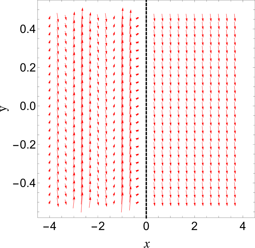
Figure 1: (Color online)The probability density $\rho$ (left) and the vector plot of the corresponding probability current density $\vec{J}$ (right) of the quasi-particle for $B$-case for step profiles. The two zones are distinguished by the vertical dashed line.

3.2 $E$-case

In this case, we also have the effective step scalar potential

$$\tilde{\phi}(w)=\sqrt{Q}\left[1+h\Theta(w)\right].$$ (26)

The scattering solution of Equation (14) is then

$$G_{E}(w)=\begin{cases}\begin{pmatrix}c_{1}e^{iq_{1}w}+d_{1}e^{-iq_{1}w}\\ e^{i\theta_{1}^{E}}c_{1}e^{iq_{1}w}-e^{-i\theta_{1}^{E}}d_{1}e^{-iq_{1}w}\end{pmatrix}\text{ if }w<0,\\ \begin{pmatrix}c_{2}e^{iq_{2}w}\\ e^{i\theta_{2}^{E}}c_{2}e^{iq_{2}w}\end{pmatrix}\text{ if }w>0,\end{cases}$$ (27)

where now $q_{1}$, $q_{2}$, $\theta_{1}$ and $\theta_{2}$ are given by

$$q_{1}=\sqrt{\left(\tilde{\varepsilon}_{E}-\sqrt{Q}\right)^{2}-\tilde{k}^{2}}>0, \tan\theta_{1}^{E}=\tilde{k}/q_{1},$$

$$q_{2}=\sqrt{\left(\tilde{\varepsilon}_{E}-\sqrt{Q}(1+h)\right)^{2}-\tilde{k}^{2}}, \tan\theta_{2}^{E}=\tilde{k}/q_{2}.$$ (28)

We would like to emphasize that the expressions of $q_{1}$ and $q_{2}$ here are the same as those in Equation (24). This fact is not surprising because $q_{1}$ and $q_{2}$ actually relate to the $x$-component of the total momentum of the quasi-particle in each zone. Because the expressions of these total momenta remain unchanged in either cases (as will be shown shortly below), so do $q_{1}$ and $q_{2}$.

This time, the coefficients $d_{1}$ and $c_{2}$ are given by

$$\dfrac{d_{1}}{c_{1}} = \left[\tilde{\mathcal{E}}(q_{1}-q_{2})-\sqrt{|Q|}\left(q_{1}-q_{2}+h(q_{1}+i\tilde{k})\right)\right]/D,$$

$$\dfrac{c_{2}}{c_{1}} = 2q_{1}\left[\tilde{\mathcal{E}}-\sqrt{|Q|}(1+h)\right]/D,$$

$$D = \left[\tilde{\mathcal{E}}(q_{1}+q_{2})-\sqrt{|Q|}\left(q_{1}+q_{2}+h(q_{1}-i\tilde{k})\right)\right].$$ (29)

The probability density $\rho(x)$ and the current density vector $\vec{J}$ are shown in Figure 2.

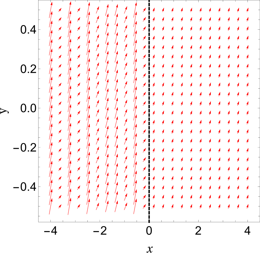
Figure 2: (Color online) The probability density $\rho$ (left) and the vector plot of the corresponding probability current density $\vec{J}$ (right) of the quasi-particle for $E$-case in step profiles. The two zones are distinguished by the vertical dashed line.

3.3 The Snell-like relation

From the above analysis, we can see that $q_{1}/r_{v}$ and $q_{2}/r_{v}(1+h)$ play the roles of $x$-momenta in the left and right zones, respectively. Thus, we deduce the case-independent total momentum in each zone

$$|\vec{P}| = \sqrt{k^{2}+\dfrac{q_{1}^{2}}{r_{v}^{2}}}=\sqrt{\dfrac{\varepsilon^{2}-r_{m}^{2}}{r_{v}^{2}}},$$

$$|\vec{Q}| = \sqrt{\left(k-\dfrac{hr_{A}}{1+h}\right)^{2}+\left(\dfrac{q_{2}}{r_{v}(1+h)}\right)^{2}}=\sqrt{\dfrac{(\varepsilon-hr_{\phi})^{2}}{r_{v}^{2}(1+h)^{2}}-\dfrac{r_{m}^{2}}{r_{v}^{2}}}.$$ (30)

It is now natural to define the incident and refracted angles with respect to the $x$-axis as follows:

$$\sin\alpha=k/|\vec{P}|,\qquad\sin\beta=\left(k-\dfrac{hr_{A}}{1+h}\right)/|\vec{Q}|.$$ (31)

Here we consider only the quasi-particles whose energies satisfy the conditions $|\varepsilon|>r_{m}$ and $|\varepsilon-hr_{\phi}|>r_{m}(1+h)$ so that $|\vec{P}|$ and $|\vec{Q}|$ is definitely real and positive. Keeping in mind that $k$ is a quantum number of the quasi-particle, we can deduce a Snell-like relation

$$|\vec{P}|\sin\alpha=|\vec{Q}|\sin\beta+\dfrac{hr_{A}}{1+h}=k$$

$$\Leftrightarrow \sqrt{\dfrac{\varepsilon^{2}-r_{m}^{2}}{r_{v}^{2}}}\sin\alpha=\sqrt{\dfrac{(\varepsilon-hr_{\phi})^{2}}{r_{v}^{2}(1+h)^{2}}-\dfrac{r_{m}^{2}}{r_{v}^{2}}}\sin\beta+\dfrac{hr_{A}}{1+h}.$$ (32)

In this relation, $|\vec{P}|$ and $|\vec{Q}|$ play the roles of the indices of refraction in two zones. This is a generalized version in the sense that it takes many quantities of the physical system (Fermi velocity, rest mass, scalar, and vector potentials) into account. For comparison, when $r_{m}=r_{\phi}=r_{A}=0$, we regain the version mentioned in Equation (8) of [34] for only velocity barrier; or when $r_{m}=0$, we can deduce the Equation (10) of [62].

We can see that except for the vector potential, the other quantities do not qualitatively change the conventional pattern of the refraction. Indeed, it is the term $n_{A}\equiv hr_{A}/(1+h)$, originating from the vector potential, that gives rise to the asymmetry of the system concerning the incident angle $\alpha$, which in turn leads to some interesting properties. First, the normal incident $\alpha=0$ corresponds $\beta=\arcsin(-n_{A}/|\vec{Q}|)$, which is generally non-zero (ray (1) in Figure 3a). In contrast, for $\alpha=\arcsin(n_{A}/|\vec{P}|)$, we have $\beta=0$ (ray (2) in Figure 3a). Notably, for any ray between the rays (1) and (2), its incident angle $\alpha$ and the refracted angle $\beta$ are always opposite in sign, which mimics the effect of the negative index of refraction. Note that negative refraction index means our system is probably a Veselago lens when using two beams of Dirac electrons. Second, the ray which goes straight forward without refraction (ray (3) in Figure 3a) is no longer the normal ray, instead it corresponds to $\alpha=\beta=\arcsin[n_{A}/(|\vec{P}|-|\vec{Q}|)]$. Besides, we also draw the blue ray as the mark for the transition between $B$-case (red rays) and $E$-case (black rays). Finally, we can define the critical values $\alpha_{c}$ of the incident angle (rays (4) and (5) in Figure 3a)

$$\sin\alpha_{c,\pm}=\left(\pm|\vec{Q}|+n_{A}\right)/|\vec{P}|.$$ (33)

For incident angles $\alpha$ which are out of the range $(\alpha_{c,-},\alpha_{c,+})$, $q_{2}$ becomes purely imaginary and the wave-function to the right decays exponentially, making the refracted angle $\beta$ not well-defined any more. Thus the critical values $\alpha_{c,\pm}$ mark the total reflection, or the sharp cut-offs of the transmission probability $T$ when plotted in terms of the incident angle. The plot of $T$ as a function of $\alpha$ is also exhibited in Figure 3b, where the critical incident angles are marked by the red (for $\alpha_{c,-}$) and the black (for $\alpha_{c,+}$) dashed lines. Again, we marked the boundary between the $B$- and $E$-cases by the blue line.

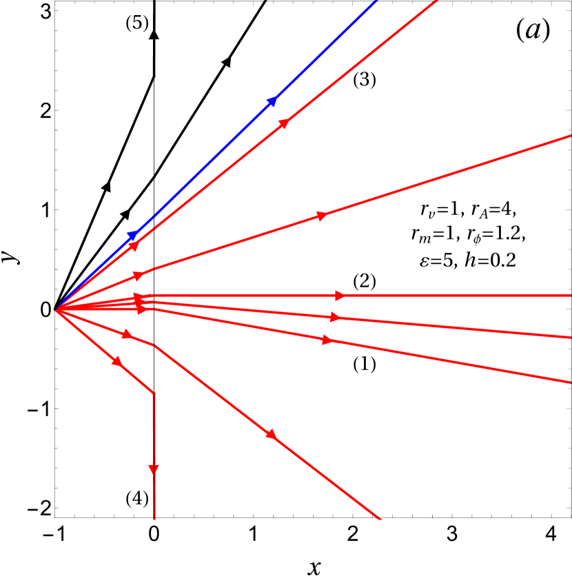
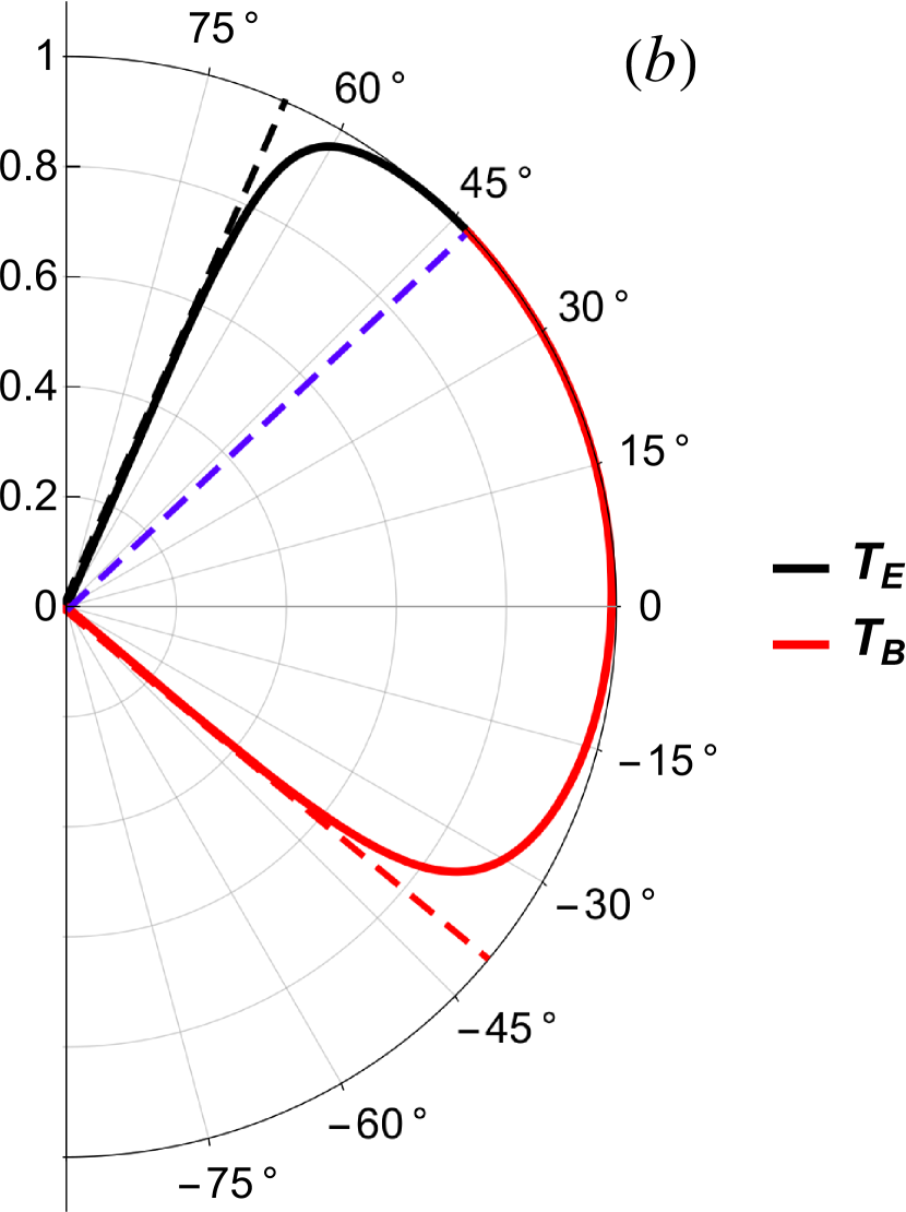
Figure 3: (Color online)(a) The illustration of some rays incident from the left at various incident angles $\alpha$: ray (1) with $\alpha=0^{o}$, $\beta\approx-10^{o}$; ray (2) with $\alpha\approx 8^{o}$, $\beta=0^{o}$; ray (3) with $\alpha=\beta\approx 39^{o}$; ray (4) with $\alpha=\alpha_{c,-}\approx-40^{o}$, $\beta=-90^{o}$; ray (5) with $\alpha=\alpha_{c,+}\approx 67^{o}$, $\beta=90^{o}$. (b) The plot of transmission probability $T$ as a function of $\alpha$ along with some dashed marking lines. In these figures, the red for $B$-case while the black for the $E$-case, and the blue for the boundary between them.

4 Multi-barrier profiles and SUSY transfer matrix method

We are now at the position to develop our formulation for a more complex system, namely a multi-barrier setup as illustrated in Figure 4. Such a configuration can be parameterized as follows:

$$v(x)=r_{v}\left[1+h\sum_{n=0}^{N-1}\Pi\left(\dfrac{x-nl}{a}\right)\right],~{}A_{y}(x)=r_{A}/\left[1+h\sum_{n=0}^{N-1}\Pi\left(\dfrac{x-nl}{a}\right)\right]-r_{A},$$

$$\Delta(x)/2=r_{m}\left[1+h\sum_{n=0}^{N-1}\Pi\left(\dfrac{x-nl}{a}\right)\right],~{}\phi(x)=r_{\phi}\left[1+h\sum_{n=0}^{N-1}\Pi\left(\dfrac{x-nl}{a}\right)\right]-r_{\phi},$$ (34)

where $\Pi(x)$ is the Heaviside Pi function, $N$ is the number of barriers, $l=a+b$ is the spatial period with $a$, $b$ are the widths of the barrier and the well, respectively. For the sake of convenience, we formally divide the material sheet into $2N+2$ zones which are denoted as below:

• The in-zone is labeled by $j=1$;

• The barriers are assigned to $j=2,4,6,\dots,2N$;

• The wells with $j=3,5,7,\dots,2N+1$ (the last well lies at the right side of the last barrier);

• The out-zone with $j=2N+2$.

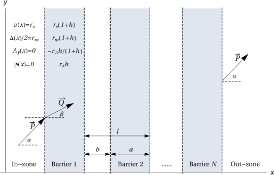
Figure 4: (Color online) Illustration of the experimental setup for the multi-barrier profiles. Each zone is distinguished with the adjacent ones by the thick, dashed, vertical lines. The barriers are shaded. The values of Fermi velocity, band gap, vector and scalar potential in each zone are also given. The beam of charged quasi-particles is assumed to move from the left in the in-zone, go through all the barriers and wells before going out in the out-zone.

We then can follow the same procedure as in Section 3. Nevertheless, we now will pay our attention to the transmission probability through the system of barriers and wells rather than the quasi-particle’s pseudo-spinor itself. To do that, a slightly modified version of the transfer matrix method (TMM) proposed in [53] will be utilized to deal with supersymmetric systems. This modified transfer matrix method, called as Supersymmetric Transfer matrix method or SUSY TMM for short, will be presented in next Subsection.

4.1 Supersymmetry Transfer matrix method (SUSY TMM)

First, we start with $B$-case and recall the necessary results of Section 3 (see C for some more details). Within $j^{th}$ zone, the intermediate pseudo-spinor $G_{B}$ at two different positions can be rewritten in the following way

$$G_{B}(w) = \begin{pmatrix}1&1\\ -ie^{i\theta_{j}}&ie^{-i\theta_{j}}\end{pmatrix}\begin{pmatrix}c_{j}e^{iq_{j}w}\\ d_{j}e^{-iq_{j}w}\end{pmatrix},$$

$$G_{B}(w+\Delta w) = \begin{pmatrix}e^{iq_{j}\Delta w}&e^{-iq_{j}\Delta w}\\ -ie^{i(\theta_{j}+q_{j}\Delta w)}&ie^{-i(\theta_{j}+q_{j}\Delta w)}\end{pmatrix}\begin{pmatrix}c_{j}e^{iq_{j}w}\\ d_{j}e^{-iq_{j}w}\end{pmatrix}.$$ (35)

where $\theta_{j}=\theta_{2}^{B}$ and $q_{j}=q_{2}$ if zone $j$ is a barrier, otherwise $\theta_{j}=\theta_{1}^{B}$ and $q_{j}=q_{1}$. Note that in terms of the auxiliary variable $w$, the effective spatial period of the system is $L=A+B$ where $A=ar_{v}^{-1}(1+h)^{-1}$ and $B=br_{v}^{-1}$ are the effective width of barrier and well, respectively. Thus we obtain the relation

$$G_{B}(w+\Delta w)=M_{j}(\Delta w)G_{B}(w)=\dfrac{1}{\cos\theta_{j}}\begin{pmatrix}\cos(\theta_{j}-q_{j}\Delta w)&-\sin(q_{j}\Delta w)\\ \sin(q_{j}\Delta w)&\cos(\theta_{j}+q_{j}\Delta w)\end{pmatrix}G_{B}(w).$$ (36)

We then can define the transfer matrix $X$ which connects $G_{B}(w=0)$ (the left edge of the first barrier) and $G_{B}(w=NL)$ (the right edge of the last well):

$$G_{B}(NL)=\left[\prod_{j=2N+1}^{2}M_{j}(z_{j})\right]G_{B}(0)=XG_{B}(0),$$ (37)

where the width of zone $j$ is $z_{j}=A$ if $j$ is even, or $z_{j}=B$ if $j$ is odd. Because all the $N$ barriers as well as all the $N$ wells are the same, we can simplify the expression of $X$ matrix as

$$X=\left[M_{3}(B)M_{2}(A)\right]^{N}.$$ (38)

The matching conditions at all the boundaries, which has been implied in Equation (37) already, can be written explicitly as

$$\begin{pmatrix}c_{2N+2}e^{iq_{1}NL}\\ -ie^{i\theta_{1}^{B}}c_{2N+2}e^{iq_{1}NL}\end{pmatrix}=\begin{pmatrix}X_{11}&X_{12}\\ X_{21}&X_{22}\end{pmatrix}\begin{pmatrix}c_{1}+d_{1}\\ -ie^{i\theta_{1}^{B}}c_{1}+ie^{-i\theta_{1}^{B}}d_{1}\end{pmatrix}.$$ (39)

Solving this gives us the expression of the transmission coefficient in this case

$$t_{B}\equiv\dfrac{c_{2N+2}}{c_{1}}=\dfrac{2\exp\left(-iq_{1}NL\right)\cos\theta_{1}^{B}}{e^{i\theta_{1}^{B}}X_{11}+e^{-i\theta_{1}^{B}}X_{22}+i(X_{12}-X_{21})}~{}.$$ (40)

Here we made use of the fact that $\det X=1$ (resulting from the property $\det M_{j}=1$) to shorten the above expression.

By the same procedure, we can obtain the transmission coefficient for $E$-case

$$t_{E}=\dfrac{2\exp\left(-iq_{1}NL\right)\cos\theta_{1}^{E}}{e^{i\theta_{1}^{E}}X_{11}+e^{-i\theta_{1}^{E}}X_{22}-(X_{12}+X_{21})},$$ (41)

where the $X$ matrix is now built from

$$M_{j}(\Delta w)=\dfrac{1}{\cos\theta_{j}}\begin{pmatrix}\cos(\theta_{j}-q_{j}\Delta w)&i\sin(q_{j}\Delta w)\\ i\sin(q_{j}\Delta w)&\cos(\theta_{j}+q_{j}\Delta w)\end{pmatrix}.$$ (42)

To sum up, with a given multi-barrier setup, we can compute the $X$ matrix and then easily obtain the transmission probability $T=|t_{B(E)}|^{2}$.

4.2 Profile of the transmission probability

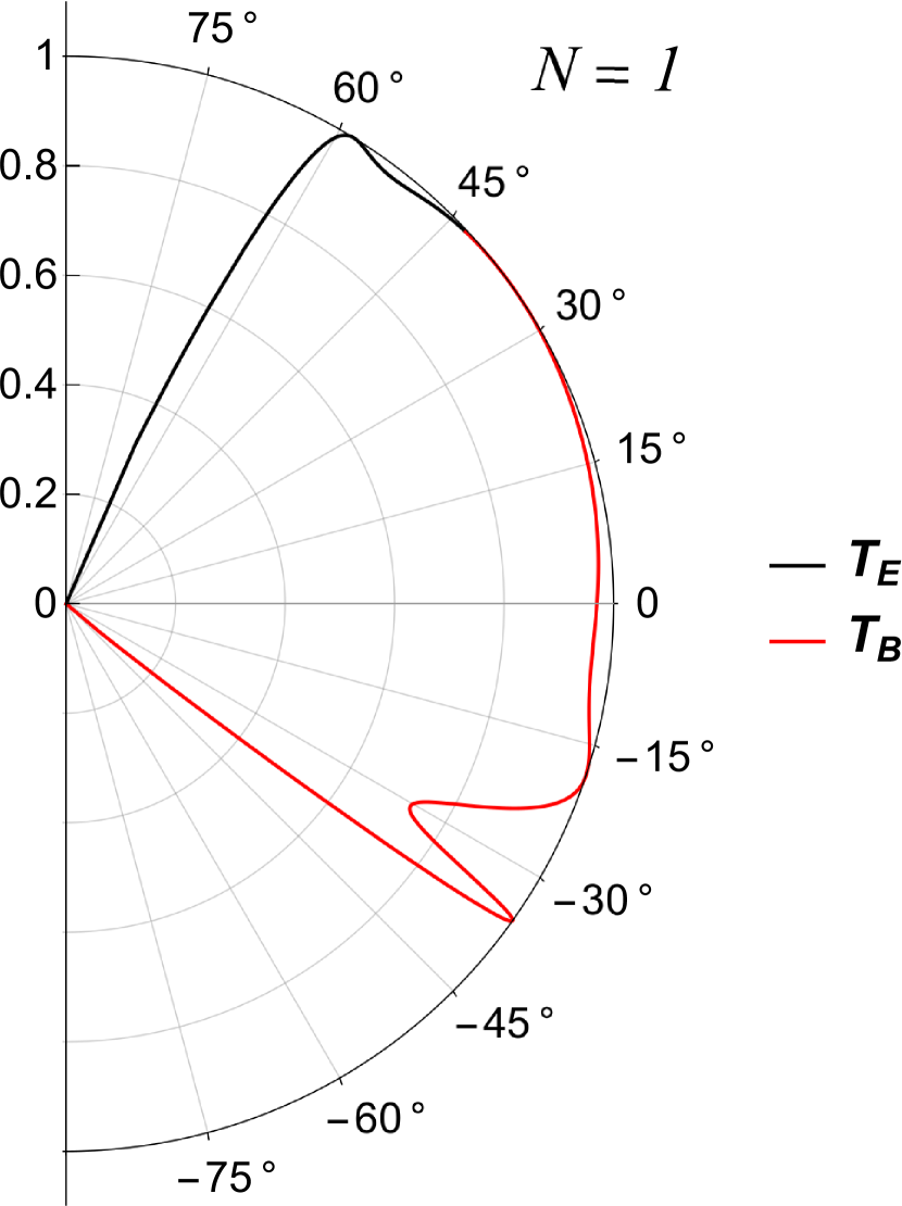
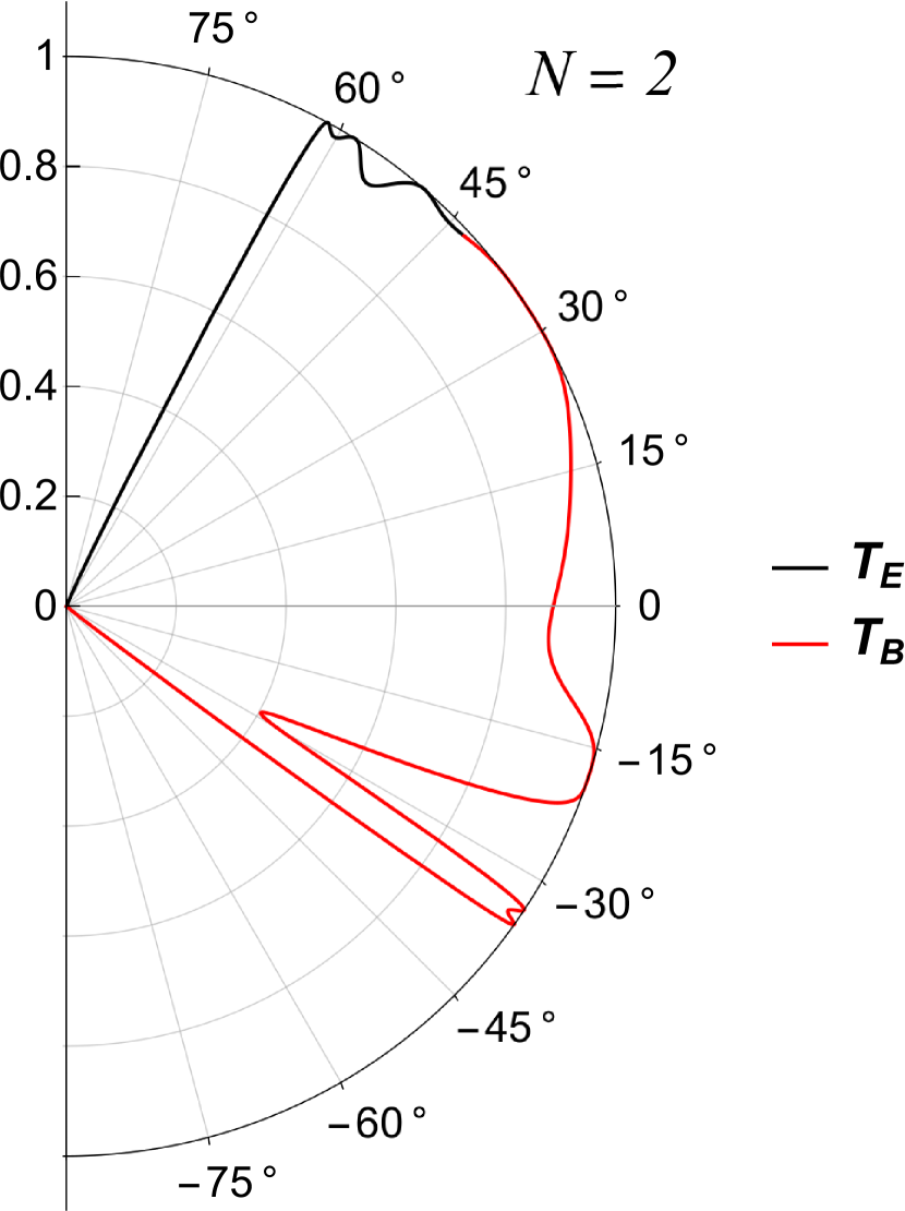
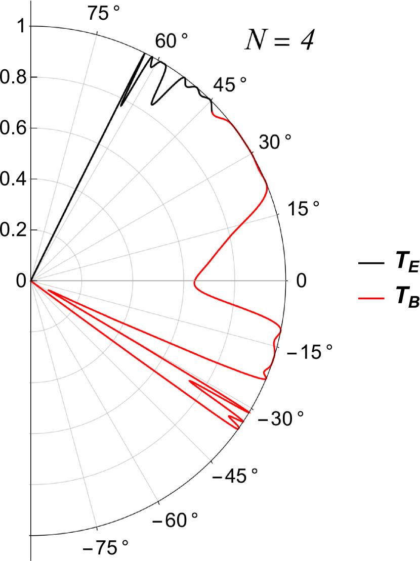
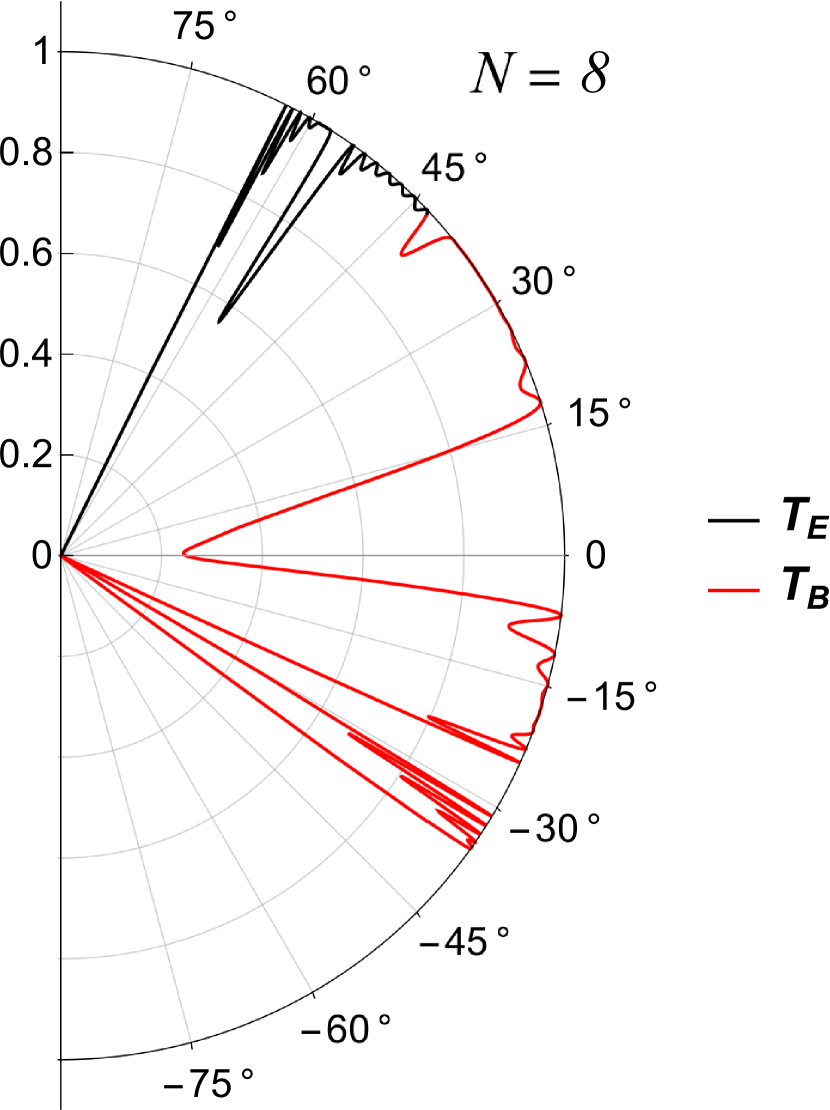
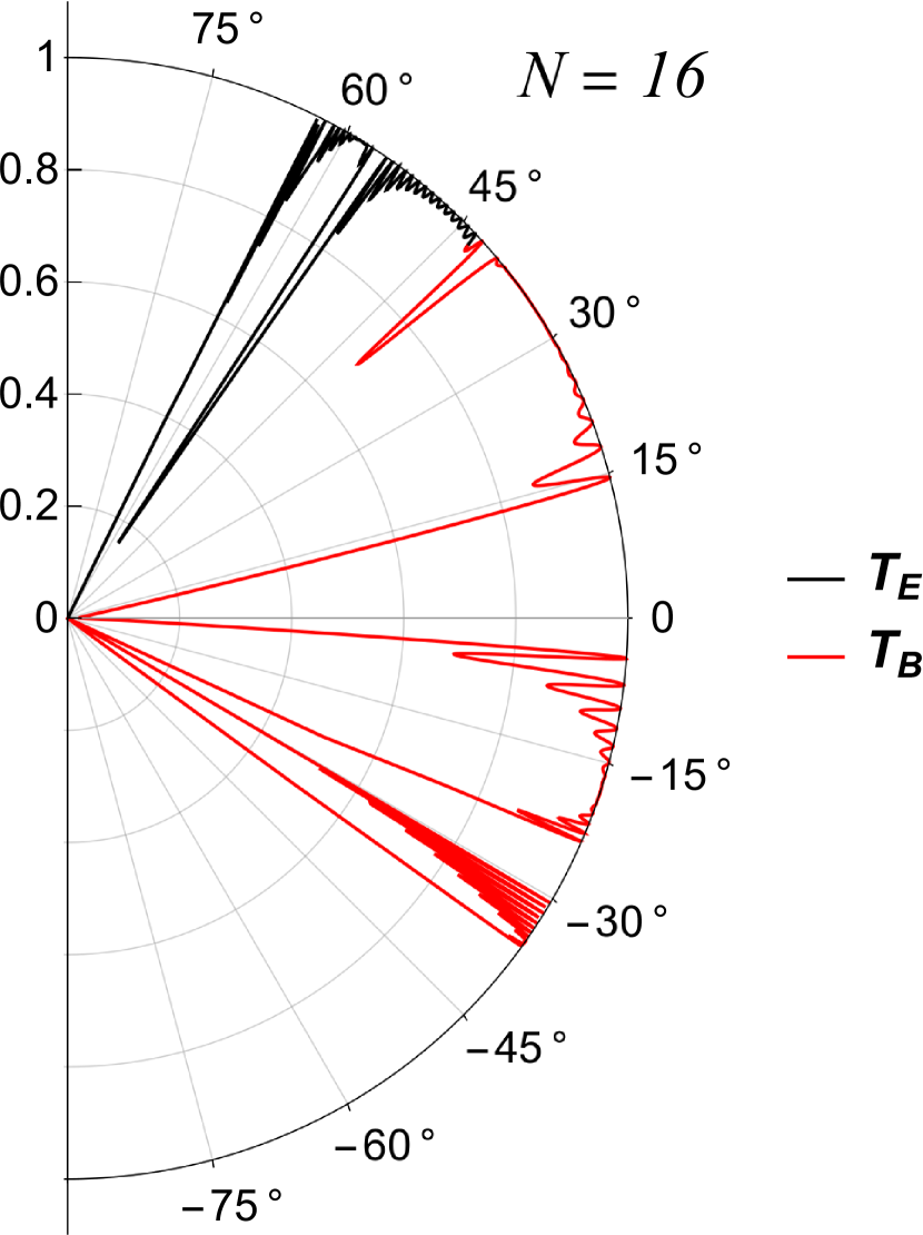
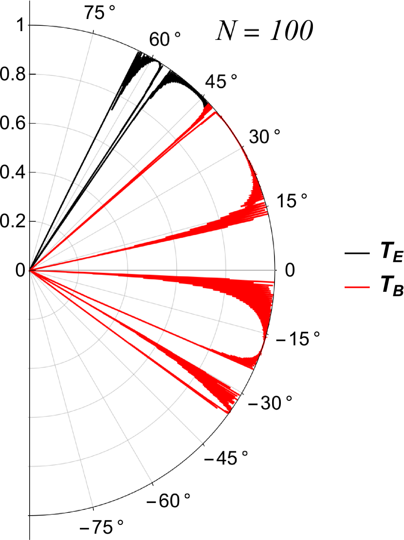
Figure 5: (Color online) Plots of the transmission probability $T$ as a function of $\alpha$ for different numbers $N$ of barriers. Except the new input parameters $b=1$ and $N=1,2,4,8,16,100$, the others are the same as in Figure 3. It is exhibited that the more barriers, the more quickly $T(\alpha)$ varies and the more transparent peaks exist. Eventually, when $N$ is very large, the transparent-bands of $\alpha$ form, interposed by the gap-bands. Note that the cut-offs $\alpha_{c,-}\approx-40^{\circ}$ and $\alpha_{c,+}\approx 67^{\circ}$ are the same as those in Figure 3 of the step profiles, no matter the number $N$ of barriers.

Figure 5 shows the transmission probability through the multi-barrier configuration as a function of the incident angle $\alpha$ with some different numbers $N=1,2,4,8,16,100$ of the barriers. We see that as $N$ increases, there are more transparent peaks where $T=1$ (this can be explained by some mathematical manipulations, see D for details) while some of the minima reach closely to zero. Consequently, when $N$ is large enough, we will obtain some transparent-bands (domains of $\alpha$ at which the quasi-particle can transmit completely through the system), distinguished to each other by the angular gap-bands where the transmission of the quasi-particle is almost banned. Note that the plots in Figure 5 use the same parameters as in Figure 3 and we can observe the same cut-offs $\alpha_{c,-}\approx-40^{\circ}$ and $\alpha_{c,+}\approx 67^{\circ}$. So the number $N$ of barriers does nothing with these cut-offs, apart from making them sharper, as expected. This means to manipulate the angular positions of these cut-offs, we have to tune the other system’s parameters instead. Also because of the optic-like behavior of Dirac electron in the situation of single barrier $N=1$, the large-$N$ system could be a Veselago lens or Fabry–-Pérot cavity (see Reference [63] and references therein for examples).

5 Discussion on Klein tunnelling

Finally, we examine the Klein tunnelling in multi-barrier configuration. More particularly, we focus on whether the transmission probability is unity when the incident wave comes at the right angle $\alpha=0$.

First, we consider the simplest situation of massless Dirac fermion and no vector potential, i.e. $r_{m}=-q_{m}=0$ and $r_{A}=-q_{A}=0$. Then because $|q_{\phi}|>|q_{m}|$, a Dirac fermion incident with $\alpha=0$ behaves as in $E$-case. Besides, both $q_{1}=|\varepsilon|$ and $q_{2}=|\varepsilon-r_{\phi}h|$ are real while it follows from Equation (3.2) that $\theta_{1}^{E}=\theta_{2}^{E}=0$. All of these simplify the expression of the transmission coefficient at the right angle:

$$t_{E}(\alpha=0)=e^{i(q_{2}-q_{1})Nw_{0}}.$$ (43)

So when the quasi-particle is massless and does not experience a vector potential, the transmission probability at the right angle is always unity, $T(\alpha=0)=|t_{E}(\alpha=0)|^{2}=1$, regardless how high or how long the scalar potential- and velocity-barriers are as well as the number of barriers. This is a manifestation of the Klein tunnelling [14].

Next, we move to the situation in which either $r_{m}$ or $r_{A}$ or both of them do(es) not vanish. To analyze this situation, we calculate the transmission probability $T$ when changing the value of $r_{m}$ (see Figure 6) or $r_{A}$ (see Figure 7) and keeping the others fixed.

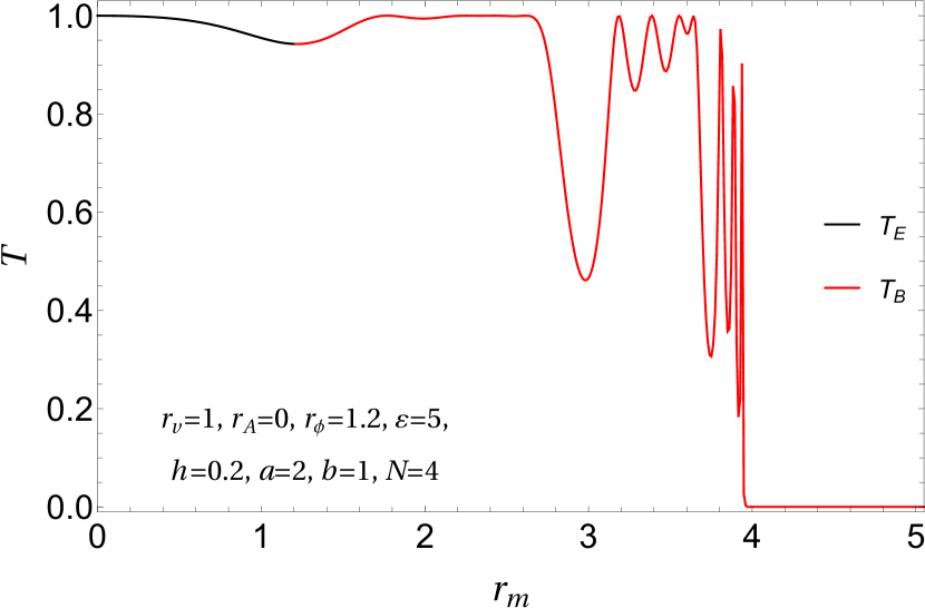
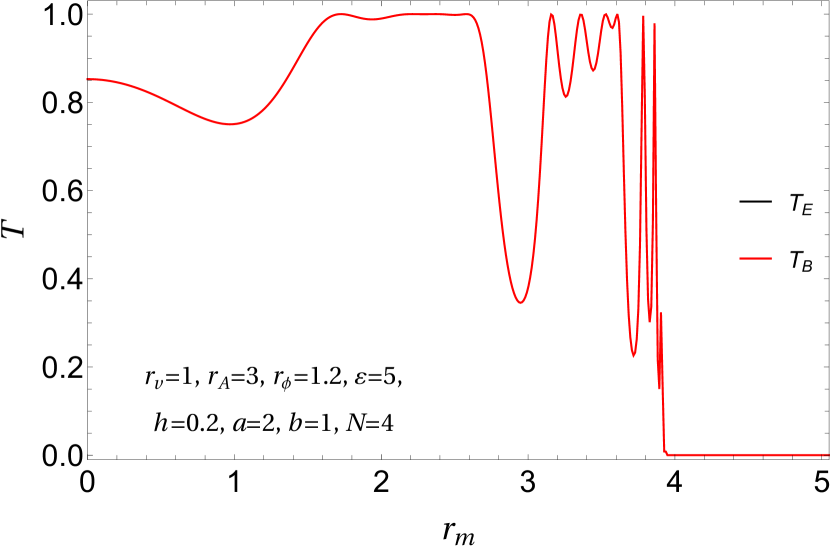
Figure 6: (Color online) Plots of the transmission probability as a function of $r_{m}$ while $r_{A}=0$ (left) or $r_{A}\neq 0$ (right). Other parameters are: $r_{v}=1$, $r_{\phi}=1.2$, $\varepsilon=5$, $h=0.2$, $a=2$, $b=1$, $N=4$.

As can been seen from the figures, we have $T=1$ when $r_{m}=r_{A}=0$ as expected. Notably, the transmission probability can also be unity with many other pairs of values $(r_{m},r_{A})$. In comparison with the conclusion in [54], in which the authors claimed that the effective mass and the vector potential can prevent the Klein tunnelling while the Fermi velocity and the scalar potential can not, our results in this work showed a bit more general conclusion that the Klein tunnelling can resurge even when either the effective rest mass of the quasi-particle or the vector potential or both of them present(s). Moreover, we can again identify the cut-offs, points at which the transmission probability suddenly drops to almost zero because the wave function of the quasi-particle becomes exponentially decaying upon transporting through the barriers. These cut-offs may be useful for controlling, i.e turning on and off, the currents of charged quasi-particles through the multi-barrier system, which is promising for electronic applications.

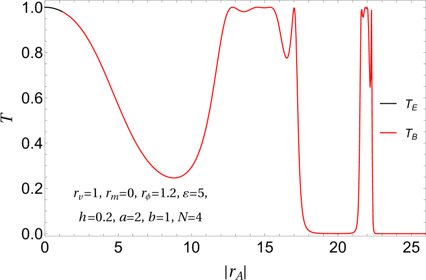
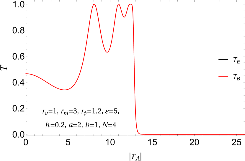
Figure 7: (Color online) Plots of the transmission probability as a function of $r_{A}$ while $r_{m}=0$ (left) or $r_{m}\neq 0$ (right). Other parameters are: $r_{v}=1$, $r_{\phi}=1.2$, $\varepsilon=5$, $h=0.2$, $a=2$, $b=1$, $N=4$.

6 Conclusion

In this work, a system of a $2D$ Dirac material sheet with step and multi-barrier profiles of Fermi velocity, effective mass, magnetic and electric fields has been analysed. Such a system can be experimentally produced using an electric cavity, a series of in-plane electrodes, superconducting materials combined with an appropriate strain engineering. We used the supersymmetric formalism, in which we took a suitable ansatz into account, to obtain the analytical expression of the wave function in terms of the quasi-particle’s energy in the case of step profiles. Then, we developed the method further by integrating it with the transfer matrix method (that we called SUSY TMM). This approach proved its usefulness for multi-barrier profiles, as it gave us a straightforward way to calculate the transmission probability of the quasi-particle transporting through the system. Considering the simple situation of step profiles allowed us to deduce a Snell-like relation for the transportation of the charged quasi-particle between two different zones of the sheet. The observation of optic-like behaviour of quasi-particle in our system suggests that our system could be used as Veselago lens. Meanwhile the multi-barrier system may be a system of Veselago lens or a Fabry-–Pérot cavity. Then the calculations for multi-barrier profiles revealed the tendency of the transmission probability when the number of barriers increases: when there are a lot of barriers, we will achieve a band-like pattern. This pattern consists of angular domains in which the transmission is highly perfect ($T>0.9$), separated by angular gaps in which the transmission is mostly banned ($T<0.1$). Also, we successfully reproduced the Klein tunnelling and reclaimed the uselessness of the Fermi velocity and scalar potential barriers in suppressing this effect. Further, we showed that even with the presence of the effective mass and the vector potential, the Klein tunnelling may still exist. Last but not least, our examination pointed out that the cut-offs in the angular distribution of the transmission probability can be manipulated by some of the parameters of the system, suggesting the potential applications in electronics. We believe that our results exhibited in this work are useful in both methodological as well as practical aspects. In the spirit of References [64, 65, 66, 59, 67, 68, 69], the similar framework may be developed for other geometrical forms of $2D$ Dirac materials such as fullerene, carbon nanotube, carbon nanohorn, carbon pseudosphere, etc. or bilayer, multilayer graphene or even organic Dirac materials with titled Dirac cone.

Author contribution statement

All authors contributed equally to the paper. All the authors have read and approved the final manuscript.

Appendix A The pseudo-spinor rotations

A general rotation $U(\alpha,\beta,\gamma)$ of the pseudo-spinor has the form

$$K(w)=UG(w)=\exp\left[\alpha/2\left(\sigma_{y}\cos\beta+\sigma_{z}\sin\beta\cos\gamma+\sigma_{x}\sin\beta\sin\gamma\right)\right]G(w),$$ (44)

where $\alpha$, $\beta$ and $\gamma$ are the three degrees of freedom (the fourth one is canceled by imposing the constraint $\det U=1$). Using this rotation, we can transform the equation for $K(w)$ into an equation for $G(w)$

$$\left\{-i\sigma_{x}\partial_{w}+\sigma_{y}\left[\tilde{k}+\tilde{A}(w)\right]+\sigma_{z}\tilde{\Delta}(w)/2+\tilde{\phi}(w)-\tilde{\varepsilon}\right\}G(w)=0,$$ (45)

with

$$\tilde{A}(w)=\bigg{[}\sinh^{2}\dfrac{\alpha}{2}\sin^{2}\beta\left(iq_{\phi}\sin 2\gamma-q_{v}(k+A_{0})\cos 2\gamma\right)$$

$$\qquad\qquad+\sinh^{2}\dfrac{\alpha}{2}\left(\dfrac{1}{2}q_{v}(k+A_{0})\cos 2\beta+q_{m}\sin 2\beta\cos\gamma\right)$$

$$\qquad\qquad+\sinh\alpha(q_{\phi}\cos\beta+iq_{m}\sin\beta\sin\gamma)+\dfrac{1}{4}q_{v}(k+A_{0})(1+3\cosh\alpha)\bigg{]}p(w),$$

$$\tilde{\phi}(w)=\bigg{[}\sinh^{2}\dfrac{\alpha}{2}\sin^{2}\beta(q_{\phi}\cos 2\gamma-iq_{v}(k+A_{0})\sin 2\gamma)$$

$$\qquad\qquad+\sinh\alpha(q_{v}(k+A_{0})\cos\beta+q_{m}\sin\beta\cos\gamma)$$

$$\qquad\qquad+\sinh^{2}\dfrac{\alpha}{2}\left(\dfrac{1}{2}q_{\phi}\cos 2\beta+iq_{m}\sin 2\beta\sin\gamma\right)+\dfrac{1}{4}q_{\phi}(1+3\cosh\alpha)\bigg{]}p(w),$$

$$\dfrac{\tilde{\Delta}(w)}{2}=\bigg{[}\sinh^{2}\dfrac{\alpha}{2}\left(q_{v}(k+A_{0})\sin 2\beta\cos\gamma-iq_{\phi}\sin 2\beta\sin\gamma-q_{m}\cos 2\beta\right)$$

$$\qquad\qquad+\sinh\alpha\sin\beta\left(q_{\phi}\cos\gamma-iq_{v}(k+A_{0})\sin\gamma\right)+\cosh^{2}\dfrac{\alpha}{2}q_{m}\bigg{]}p(w)$$

$$\qquad\qquad+\sinh\alpha\sin\beta\left((\phi_{0}-\varepsilon)\cos\gamma-iq_{v}q_{A}\sin\gamma\right)$$

$$\qquad\qquad+\sinh^{2}\dfrac{\alpha}{2}\sin 2\beta(q_{v}q_{A}\cos\gamma-i(\phi_{0}-\varepsilon)\sin\gamma),$$

$$\tilde{k}=+\sinh^{2}\dfrac{\alpha}{2}\left[\dfrac{1}{2}q_{v}q_{A}\cos 2\beta-\sin^{2}\beta(q_{v}q_{A}\cos 2\gamma-i(\phi_{0}-\varepsilon)\sin 2\gamma)\right]$$

$$\qquad\qquad+(\phi_{0}-\varepsilon)\sinh\alpha\cos\beta+\dfrac{1}{4}q_{v}q_{A}(1+3\cosh\alpha),$$

$$\tilde{\varepsilon}=-\sinh^{2}\dfrac{\alpha}{2}\left[\dfrac{1}{2}(\phi_{0}-\varepsilon)\cos 2\beta+\sin^{2}\beta\left((\phi_{0}-\varepsilon)\cos 2\gamma-iq_{v}q_{A}\sin 2\gamma\right)\right]$$

$$\qquad\qquad-q_{v}q_{A}\sinh\alpha\cos\beta-\dfrac{1}{4}(\phi_{0}-\varepsilon)(1+3\cosh\alpha).$$ (46)

To obtain the $B$-case, we can use the rotation $U_{B}(\alpha^{B},\beta^{B},\gamma^{B})$ with

$$\cosh\dfrac{\alpha^{B}}{2} = \dfrac{s_{1}^{B}\left[(k+A_{0})q_{v}+\sqrt{-Q}\right]-is_{2}^{B}(q_{m}+q_{\phi})}{2},\qquad\qquad\qquad\quad\qquad~{}~{}$$

$$\cos\beta^{B} = i\dfrac{s_{2}^{B}\left[(k+A_{0})q_{v}-\sqrt{-Q}\right]+is_{1}^{B}(q_{m}+q_{\phi})}{2\sinh\dfrac{\alpha^{B}}{2}},$$

$$\cos\gamma^{B} = \dfrac{s_{1}^{B}\left[(k+A_{0})q_{v}+\sqrt{-Q}\right]+is_{2}^{B}(q_{m}+q_{\phi})}{2\sin\beta^{B}\sinh\dfrac{\alpha^{B}}{2}}.$$ (47)

For $E$-case, the rotation $U_{E}$ is now determined by

$$\cosh\dfrac{\alpha^{E}}{2} = \dfrac{i(k+A_{0})q_{v}(s_{1}^{E}+s_{2}^{E})-\sqrt{Q}(s_{1}^{E}-s_{2}^{E})+(q_{m}+q_{\phi})(s_{1}^{E}-s_{2}^{E})}{2},$$

$$\cos\beta^{E} = i\dfrac{i(k+A_{0})q_{v}(s_{1}^{E}-s_{2}^{E})-\sqrt{Q}(s_{1}^{E}+s_{2}^{E})-(q_{m}+q_{\phi})(s_{1}^{E}+s_{2}^{E})}{2\sinh\dfrac{\alpha^{E}}{2}},$$

$$\cos\gamma^{E} = \dfrac{i(k+A_{0})q_{v}(s_{1}^{E}+s_{2}^{E})-\sqrt{Q}(s_{1}^{E}-s_{2}^{E})-(q_{m}+q_{\phi})(s_{1}^{E}-s_{2}^{E})}{2\sin\beta^{E}\sinh\dfrac{\alpha^{E}}{2}}.$$ (48)

Here, the factors $s$ are given by

$$(s_{1,2}^{B})^{2}=\dfrac{\sqrt{\pm 1}}{\sqrt{\mp 1}}\left[2(q_{m}+q_{\phi})\sqrt{Q}\right]^{-1}\times\qquad\qquad\qquad\qquad\qquad\qquad\qquad\qquad\qquad\qquad\qquad\qquad$$

$$\dfrac{\sqrt{q_{v}\left[(k+A_{0})q_{v}\mp\sqrt{-Q}\right]\left[(\varepsilon-\phi_{0})(k+A_{0})+q_{A}(q_{m}+q_{\phi})\right]+(\varepsilon-\phi_{0})q_{m}(q_{m}+q_{\phi})}}{\sqrt{q_{v}\left[(k+A_{0})q_{v}\pm\sqrt{-Q}\right]\left[(\varepsilon-\phi_{0})(k+A_{0})+q_{A}(q_{m}+q_{\phi})\right]+(\varepsilon-\phi_{0})q_{m}(q_{m}+q_{\phi})}},\quad$$

$$(s_{1,2}^{E})^{2}=\dfrac{\sqrt{\pm 1}}{\sqrt{\mp 1}}\left[4(q_{m}+q_{\phi})\sqrt{Q}\right]^{-1}\times\qquad\qquad\qquad\qquad\qquad\qquad\qquad\qquad\qquad\qquad\qquad\qquad$$

$$\dfrac{\sqrt{q_{v}\left[(k+A_{0})q_{v}\mp i\sqrt{Q}\right]\left[(\varepsilon-\phi_{0})(k+A_{0})+q_{A}(q_{m}+q_{\phi})\right]+(\varepsilon-\phi_{0})q_{m}(q_{m}+q_{\phi})}}{\sqrt{q_{v}\left[(k+A_{0})q_{v}\pm i\sqrt{Q}\right]\left[(\varepsilon-\phi_{0})(k+A_{0})+q_{A}(q_{m}+q_{\phi})\right]+(\varepsilon-\phi_{0})q_{m}(q_{m}+q_{\phi})}}.\quad$$ (49)

Appendix B The formulae of the probability density and the probability current density

For both the $B$- and $E$-cases, the expressions of the probability density $\rho$ and the probability current density $\vec{J}$ are given by [54]

$$\rho^{B,E}(x) = \Psi^{\dagger}(x,y)\Psi(x,y)=\dfrac{1}{v(x)}G_{B,E}^{\dagger}(w(x))U_{B,E}^{\dagger}U_{B,E}G_{B,E}(w(x)),$$

$$J_{x}^{B,E} = v(x)\Psi^{\dagger}(x,y)\sigma_{x}\Psi(x,y)=G_{B,E}^{\dagger}(w(x))U_{B,E}^{\dagger}\sigma_{x}U_{B,E}G_{B,E}(w(x)),$$

$$J_{y}^{B,E} = v(x)\Psi^{\dagger}(x,y)\sigma_{y}\Psi(x,y)=G_{B,E}^{\dagger}(w(x))U_{B,E}^{\dagger}\sigma_{y}U_{B,E}G_{B,E}(w(x)).$$ (50)

Appendix C Variable-changing for multi-barrier system

The auxiliary variable is

$$w = \int_{x_{0}-a/2}^{x}\dfrac{\text{d}u}{r_{v}\left[1+h\sum_{n=0}^{N-1}\Pi\left(\dfrac{x-nl}{a}\right)\right]}$$ (51)

$$= \dfrac{1}{r_{v}}\times\begin{cases}x+a/2\qquad\qquad\qquad\qquad\qquad~{}\text{ in zone $j=1$;}\\ \dfrac{x+a/2}{1+h}+(j/2-1)\dfrac{bh}{1+h}~{}~{}~{}~{}~{}~{}~{}\text{ in zone $j=2,4,\dots,2N$;}\\ x+a/2+a\left(1-\dfrac{h(j-1)/2}{1+h}\right)~{}\text{ in zone $j=3,5,\dots,2N+1$;}\\ x+a/2+a\left(1-\dfrac{Nh}{1+h}\right)\qquad~{}~{}\text{ in zone $j=2N+2$.}\end{cases}$$

We can rewrite the above quantities to show that they satisfy the ansatz (2) with

$$q_{v}=-r_{v}<0,\quad q_{A}=-r_{A},\quad q_{m}=-r_{m}\leq 0,\quad q_{\phi}=-r_{\phi},$$

$$p(w)=-\left[1+h\sum_{n=0}^{N-1}\Pi\left(\dfrac{w-nL}{A}-\dfrac{1}{2}\right)\right]<0.$$ (52)

Appendix D The increase in the number of transparent peaks when $N$ increases

To explain the increase in the number of transparent peaks when the number $N$ of barriers increases, we re-examine the transfer matrix $X$. Because, in principle, all $2\times 2$ matrices can be uniquely decomposed into the Pauli matrices $\sigma_{j}$ ($j=1,2,3$) and the identity matrix $\mathbb{I}$, we have

$$X=[M_{3}M_{2}]^{N} = [A_{0}\mathbb{I}+A_{1}\sigma_{1}+A_{2}\sigma_{2}+A_{3}\sigma_{3}]^{N}$$ (53)

$$= \left[u_{0}+\cos(u)+i\sin(u)\left(\dfrac{u_{1}}{u}\sigma_{1}+\dfrac{u_{2}}{u}\sigma_{2}+\dfrac{u_{3}}{u}\sigma_{3}\right)\right]^{N}$$

where we introduced the vector $\vec{u}=(u_{1},u_{2},u_{3})$ whose components satisfy the following relations

$$iu_{j}\sin(u)/u=A_{j},\qquad j=1,2,3.$$ (54)

Here $u=\sqrt{u_{1}^{2}+u_{2}^{2}+u_{3}^{2}}$ is the length of $\vec{u}$ and in this situation $\cos(u)=A_{0}-u_{0}$. Then, according to Euler’s identity for matrix, $X$ can be rewritten

$$X = \left[u_{0}+e^{i\vec{u}\cdot\vec{\sigma}}\right]^{N}$$ (55)

$$= \sum_{n=0}^{N}u_{0}^{N-n}e^{in\vec{u}\cdot\vec{\sigma}}$$

$$= \sum_{n=0}^{N}u_{0}^{N-n}\left[\cos(nu)+i\sin(nu)\left(\dfrac{u_{1}}{u}\sigma_{1}+\dfrac{u_{2}}{u}\sigma_{2}+\dfrac{u_{3}}{u}\sigma_{3}\right)\right]$$

$$= X_{0}(N)+i\left(\dfrac{u_{1}}{u}\sigma_{1}+\dfrac{u_{2}}{u}\sigma_{2}+\dfrac{u_{3}}{u}\sigma_{3}\right)X_{\sigma}(N)$$

where

$$X_{0}(N) = \sum_{n=0}^{N}u_{0}^{N-n}\cos(nu)=\frac{\cos(Nu)-u_{0}\cos[(N+1)u]-u_{0}^{N+1}\cos(u)+u_{0}^{N+2}}{\left(e^{iu}-u_{0}\right)\left(e^{-iu}-u_{0}\right)},$$

$$X_{\sigma}(N) = \sum_{n=0}^{N}u_{0}^{N-n}\sin(nu)=\frac{\sin(Nu)-u_{0}\sin[(N+1)u]+u_{0}^{N+1}\sin(u)}{\left(e^{iu}-u_{0}\right)\left(e^{-iu}-u_{0}\right)}.$$ (56)

Or in matrix form, we have

$$X=\begin{pmatrix}X_{0}(N)+iX_{\sigma}(N)u_{3}/u&iX_{\sigma}(N)u_{1}/u+X_{\sigma}(N)u_{2}/u\\ iX_{\sigma}(N)u_{1}/u-X_{\sigma}(N)u_{2}/u&X_{0}(N)-iX_{\sigma}(N)u_{3}/u\end{pmatrix}.$$ (57)

Now, we can rewrite transmission probabilities in terms of $N$ for both cases

$$T_{B}(N)=|t_{B}|^{2} = \left|X_{0}(N)-X_{\sigma}(N)\tan\theta_{1}^{B}\dfrac{u_{3}}{u}+i\dfrac{X_{\sigma}(N)}{\cos\theta_{1}^{B}}\dfrac{u_{2}}{u}\right|^{-2},$$

$$T_{E}(N)=|t_{E}|^{2} = \left|X_{0}(N)-X_{\sigma}(N)\tan\theta_{1}^{E}\dfrac{u_{3}}{u}-i\dfrac{X_{\sigma}(N)}{\cos\theta_{1}^{E}}\dfrac{u_{1}}{u}\right|^{-2}.$$ (58)

We can see that the number $N$ of barriers plays the role of a factor in the phase of the trigonometric functions, making the transmission probability $T$ oscillates more rapidly with respect to the incident angle $\alpha$ (keep in mind that all $u,u_{1},u_{2},u_{3},\theta_{1}^{B},\theta_{1}^{E}$ depend on $\alpha$). The obvious consequence is that when $N$ is doubled, the number of transparent peaks is roughly doubled as well, as observed in the Figure 5.

References

- [1] K. S. Novoselov, A. K. Geim, S. V. Morozov, D. Jiang, M. I. Katsnelson, I. V. Grigorieva, S. V. Dubonos, A. A. Firsov, Two-dimensional gas of massless dirac fermions in graphene, Nature 438 (7065) (2005) 197.
- [2] C.-C. Liu, H. Jiang, Y. Yao, Low-energy effective hamiltonian involving spin-orbit coupling in silicene and two-dimensional germanium and tin, Physical Review B 84 (2011) 195430.
- [3] C.-C. Liu, W. Feng, Y. Yao, Quantum spin hall effect in silicene and two-dimensional germanium, Physical Review Letters 107 (2011) 076802.
- [4] T. O. Wehling, A. M. Black-Schaffer, A. V. Balatsky, Dirac materials, Advances in Physics 63 (1) (2014) 1–76.
- [5] L. M. Woods, D. A. R. Dalvit, A. Tkatchenko, P. Rodriguez-Lopez, A. W. Rodriguez, R. Podgornik, Materials perspective on casimir and van der waals interactions, Rev. Mod. Phys. 88 (2016) 045003.
- [6] Y. Zhang, Y.-W. Tan, H. L. Stormer, P. Kim, Experimental observation of the quantum hall effect and berry’s phase in graphene, Nature 438 (7065) (2005) 201.
- [7] A. H. Castro Neto, F. Guinea, N. M. R. Peres, K. S. Novoselov, A. K. Geim, The electronic properties of graphene, Reviews of Modern Physics 81 (2009) 109.
- [8] M. Tahir, U. Schwingenschlögl, Valley polarized quantum hall effect and topological insulator phase transitions in silicene, Scientific reports 3 (2013) 1075.
- [9] M. Tahir, A. Manchon, K. Sabeeh, U. Schwingenschlögl, Quantum spin/valley hall effect and topological insulator phase transitions in silicene, Applied Physics Letters 102 (16) (2013) 162412.
- [10] L. Matthes, O. Pulci, F. Bechstedt, Massive dirac quasiparticles in the optical absorbance of graphene, silicene, germanene, and tinene, Journal of Physics: Condensed Matter 25 (39) (2013) 395305.
- [11] J. Wang, S. Deng, Z. Liu, Z. Liu, The rare two-dimensional materials with Dirac cones, National Science Review 2 (1) (2015) 22–39.
- [12] M. I. Katsnelson, K. S. Novoselov, A. K. Geim, Chiral tunnelling and the klein paradox in graphene, Nature Physics 2 (2006) 620–625.
- [13] O. Klein, Die reflexion von elektronen an einem potentialsprung nach der relativistischen dynamik von dirac, Zeitschrift für Physik 53 (3-4) (1929) 157–165.
- [14] A. Calogeracos, N. Dombey, History and physics of the klein paradox, Contemporary Physics 40 (5) (1999) 313–321.
- [15] C. J. Tabert, E. J. Nicol, Magneto-optical conductivity of silicene and other buckled honeycomb lattices, Physical Review B 88 (2013) 085434.
- [16] Ş Kuru, J. Negro, L. M. Nieto, Exact analytic solutions for a dirac electron moving in graphene under magnetic fields, Journal of Physics: Condensed Matter 21 (45) (2009) 455305.
- [17] M. R. Masir, P. Vasilopoulos, F. M. Peeters, Graphene in inhomogeneous magnetic fields: bound, quasi-bound and scattering states, Journal of Physics: Condensed Matter 23 (31) (2011) 315301.
- [18] P. Roy, T. K. Ghosh, K. Bhattacharya, Localization of dirac-like excitations in graphene in the presence of smooth inhomogeneous magnetic fields, Journal of Physics: Condensed Matter 24 (5) (2012) 055301.
- [19] C. A. Downing, M. E. Portnoi, Massless dirac fermions in two dimensions: Confinement in nonuniform magnetic fields, Physical Review B 94 (2016) 165407.
- [20] D.-N. Le, P.-S. Luu, T.-S. Ha, N.-H. Phan, V.-H. Le, Bound states of (2+1)-dimensional massive dirac fermions in a lorentzian-shaped inhomogeneous perpendicular magnetic field, Physica E: Low-dimensional Systems and Nanostructures 116 (2020) 113777.
- [21] M. O. Goerbig, Electronic properties of graphene in a strong magnetic field, Rev. Mod. Phys. 83 (2011) 1193–1243.
- [22] M. R. Masir, P. Vasilopoulos, F. M. Peeters, Wavevector filtering through single-layer and bilayer graphene with magnetic barrier structures, Applied Physics Letters 93 (24) (2008) 242103.
- [23] L. Dell’Anna, A. De Martino, Multiple magnetic barriers in graphene, Phys. Rev. B 79 (2009) 045420.
- [24] H. Nguyen-Truong, V. V. On, M.-F. Lin, Optical absorption spectra of Xene and Xane (X = silic, german, stan), Journal of Physics: Condensed Matter 33 (35) (2021) 355701.
- [25] N. D. Drummond, V. Zólyomi, V. I. Fal’ko, Electrically tunable band gap in silicene, Phys. Rev. B 85 (2012) 075423.
- [26] D.-N. Le, V.-H. Le, P. Roy, Modulation of landau levels and de haas-van alphen oscillation in magnetized graphene by uniaxial tensile strain/ stress, Journal of Magnetism and Magnetic Materials (2020) 167473.
- [27] M. A. H. Vozmediano, F. de Juan, A. Cortijo, Gauge fields and curvature in graphene, Journal of Physics: Conference Series 129 (2008) 012001.
- [28] M. Vozmediano, M. Katsnelson, F. Guinea, Gauge fields in graphene, Physics Reports 496 (4) (2010) 109–148.
- [29] V. M. Pereira, A. H. Castro Neto, Strain Engineering of Graphene’s Electronic Structure, Physical Review Letters 103 (4) (2009) 046801.
- [30] T. Low, F. Guinea, Strain-induced pseudomagnetic field for novel graphene electronics, Nano Letters 10 (9) (2010) 3551–3554.
- [31] N. Levy, S. A. Burke, K. L. Meaker, M. Panlasigui, A. Zettl, F. Guinea, A. H. C. Neto, M. F. Crommie, Strain-Induced Pseudo-Magnetic Fields Greater Than 300 Tesla in Graphene Nanobubbles, Science 329 (5991) (2010) 544–547.
- [32] F. Guinea, M. I. Katsnelson, A. K. Geim, Energy gaps and a zero-field quantum hall effect in graphene by strain engineering, Nature Physics 6 (1) (2010) 30–33.
- [33] F. de Juan, J. L. Mañes, M. A. H. Vozmediano, Gauge fields from strain in graphene, Phys. Rev. B 87 (2013) 165131.
- [34] A. Raoux, M. Polini, R. Asgari, A. R. Hamilton, R. Fazio, A. H. MacDonald, Velocity-modulation control of electron-wave propagation in graphene, Phys. Rev. B 81 (2010) 073407.
- [35] F. M. D. Pellegrino, G. G. N. Angilella, R. Pucci, Transport properties of graphene across strain-induced nonuniform velocity profiles, Physical Review B 84 (2011) 195404.
- [36] F. de Juan, M. Sturla, M. A. H. Vozmediano, Space dependent fermi velocity in strained graphene, Physical Review Letters 108 (2012) 227205.
- [37] S. Barraza-Lopez, A. A. Pacheco Sanjuan, Z. Wang, M. Vanević, Strain-engineering of graphene’s electronic structure beyond continuum elasticity, Solid State Communications 166 (2013) 70–75.
- [38] J. V. Sloan, A. A. P. Sanjuan, Z. Wang, C. Horvath, S. Barraza-Lopez, Strain gauge fields for rippled graphene membranes under central mechanical load: An approach beyond first-order continuum elasticity, Phys. Rev. B 87 (2013) 155436.
- [39] A. A. Pacheco Sanjuan, Z. Wang, H. P. Imani, M. Vanević, S. Barraza-Lopez, Graphene’s morphology and electronic properties from discrete differential geometry, Phys. Rev. B 89 (2014) 121403.
- [40] M. Oliva-Leyva, G. G. Naumis, Generalizing the Fermi velocity of strained graphene from uniform to nonuniform strain, Physics Letters, Section A: General, Atomic and Solid State Physics 379 (40-41) (2015) 2645–2651.
- [41] C. A. Downing, M. E. Portnoi, Localization of massless Dirac particles via spatial modulations of the Fermi velocity, Journal of Physics: Condensed Matter 29 (31) (2017) 315301.
- [42] G. G. Naumis, S. Barraza-Lopez, M. Oliva-Leyva, H. Terrones, Electronic and optical properties of strained graphene and other strained 2d materials: a review, Reports on Progress in Physics 80 (9) (2017) 096501.
- [43] E. Lantagne-Hurtubise, X.-X. Zhang, M. Franz, Dispersive landau levels and valley currents in strained graphene nanoribbons, Phys. Rev. B 101 (2020) 085423.
- [44] B. Dong, W. Sun, D. Liu, N. Ma, The mechanical strain induced anomalous de haas–van alphen effect on graphene, Physica B: Condensed Matter 577 (2020) 411824.
- [45] D.-N. Le, V.-H. Le, P. Roy, Graphene under uniaxial inhomogeneous strain and an external electric field: Landau levels, electronic, magnetic and optical properties, The European Physical Journal B 93 (8) (2020) 158.
- [46] F. Zhai, X. Zhao, K. Chang, H. Q. Xu, Magnetic barrier on strained graphene: A possible valley filter, Phys. Rev. B 82 (2010) 115442.
- [47] Y. Betancur-Ocampo, P. Majari, D. Espitia, F. Leyvraz, T. Stegmann, Anomalous Floquet tunneling in uniaxially strained graphene, Physical Review B 103 (15) (2021) 155433.
- [48] P. Ghosh, P. Roy, Bound states in graphene via Fermi velocity modulation, European Physical Journal Plus 132 (1) (2017) 32.
- [49] A.-L. Phan, D.-N. Le, V.-H. Le, P. Roy, Electronic spectrum in 2d dirac materials under strain, Physica E: Low-dimensional Systems and Nanostructures 121 (2020) 114084.
- [50] R. Ghosh, (1+1)-dimensional Dirac equation in an effective mass theory under the influence of local fermi velocity.
- [51] M. Oliva-Leyva, J. E. Barrios-Vargas, G. G. de la Cruz, Effective magnetic field induced by inhomogeneous fermi velocity in strained honeycomb structures, Phys. Rev. B 102 (2020) 035447.
- [52] Ícaro S.F. Bezerra, J. R. Lima, Effects of fermi velocity engineering in magnetic graphene superlattices, Physica E: Low-dimensional Systems and Nanostructures 123 (2020) 114171.
- [53] L.-G. Wang, S.-Y. Zhu, Electronic band gaps and transport properties in graphene superlattices with one-dimensional periodic potentials of square barriers, Phys. Rev. B 81 (2010) 205444.
- [54] N. M. R. Peres, Scattering in one-dimensional heterostructures described by the dirac equation, Journal of Physics: Condensed Matter 21 (9) (2009) 095501.
- [55] V. Lukose, R. Shankar, G. Baskaran, Novel electric field effects on landau levels in graphene, Phys. Rev. Lett. 98 (2007) 116802.
- [56] F. Cooper, A. Khare, U. Sukhatme, Supersymmetry and quantum mechanics, Physics Reports 251 (5) (1995) 267 – 385.
- [57] R. Yekken, M. Lassaut, R. Lombard, Applying supersymmetry to energy dependent potentials, Annals of Physics 338 (2013) 195 – 206.
- [58] Y. Concha, A. Huet, A. Raya, D. Valenzuela, Supersymmetric quantum electronic states in graphene under uniaxial strain, Materials Research Express 5 (6) (2018) 065607.
- [59] D.-N. Le, V.-H. Le, P. Roy, Orbital magnetization in axially symmetric two-dimensional carbon allotrope: influence of electric field and geometry, Journal of Physics: Condensed Matter 32 (38) (2020) 385703.
- [60] B. Bagchi, R. Ghosh, Dirac Hamiltonian in a supersymmetric framework, Journal of Mathematical Physics 62 (7) (2021) 072101.
- [61] L. Z. Tan, C.-H. Park, S. G. Louie, Graphene dirac fermions in one-dimensional inhomogeneous field profiles: Transforming magnetic to electric field, Phys. Rev. B 81 (2010) 195426.
- [62] L. Liu, Y. X. Li, J. J. Liu, Transport properties of Dirac electrons in graphene based double velocity-barrier structures in electric and magnetic fields, Physics Letters, Section A: General, Atomic and Solid State Physics 376 (45) (2012) 3342–3350.
- [63] Q. Wilmart, S. Berrada, D. Torrin, V. H. Nguyen, G. Fève, J.-M. Berroir, P. Dollfus, B. Plaçais, A klein-tunneling transistor with ballistic graphene, 2D Materials 1 (1) (2014) 011006.
- [64] D.-N. Le, A.-L. Phan, V.-H. Le, P. Roy, Spherical fullerene molecules under the influence of electric and magnetic fields, Physica E: Low-dimensional Systems and Nanostructures 107 (2019) 60–66.
- [65] D.-N. Le, V.-H. Le, P. Roy, Electric field and curvature effects on relativistic landau levels on a pseudosphere, Journal of Physics: Condensed Matter 31 (30) (2019) 305301.
- [66] A.-L. Phan, D.-N. Le, V.-H. Le, P. Roy, The influence of electric field and geometry on relativistic landau levels in spheroidal fullerene molecules, Physica E: Low-dimensional Systems and Nanostructures 114 (2019) 113639.
- [67] D. J. Fernández, D. I. Martínez-Moreno, Bilayer graphene coherent states, The European Physical Journal Plus 135 (2020) 739.
- [68] G. Wagner, D. X. Nguyen, S. H. Simon, Transport properties of multilayer graphene, Phys. Rev. B 101 (2020) 245438.
- [69] Y. Betancur-Ocampo, E. Díaz-Bautista, T. Stegmann, Valley-dependent time evolution of coherent electron states in tilted anisotropic Dirac materials (2021) 1–13.