Long time behavior of nonlinear electromagnetic wave in vacuum beyond linear approximation

Abstract

A quantum nature of vacuum is expected to affect electromagnetic fields in vacuum as a nonlinear correction, yielding nonlinear Maxwell’s equations. We extend the finite-difference time-domain (FDTD) method in the case that the nonlinear electromagnetic Lagrangian is quartic with respect to the electric field and magnetic flux density. With this extension, the nonlinear Maxwell’s equations can be numerically solved without making any assumptions on the electromagnetic field. We demonstrate examples of self-modulations of nonlinear electromagnetic waves in a one-dimensional cavity, in particular, in a time scale beyond an applicable range of linear approximation. A momentarily small nonlinear correction can accumulate and a comparably large self-modulation can be achieved in a long time scale even though the electromagnetic field is not extremely strong. Further, we analytically approximate the nonlinear electromagnetic waves in the cavity and clarify the characteristics, for example, how an external magnetic flux density changes the self-modulations of phase and polarization.

I Introduction

In classical electromagnetism, the electromagnetic fields in vacuum are described by the linear Maxwell’s equations. In modern physics, several corrections have been proposed for the behavior of the electromagnetic fields such as the Heisenberg-Euler theory [1] based on the quantum electrodynamics, the Born-Infeld theory [2] derived by an analogy to the special theory of relativity, and the more generalized Plebański class [3]. The nonlinear correction of electromagnetic fields affects many branches of physics. For example, several calculations are performed for the interaction of strong laser beams [4][5], the radiation from pulsars and neutron stars [6] [7][8], the Wichmann-Kroll correction [9] to the Lamb shift, a photon-photon scattering [10], an interaction between a nucleus and electrons through the Uehling potential [11][12][13], a correction to the states of a hydrogen atom [14][15] [16][17], an electromagnetic effect for black holes [18][19], and a possibility of magnetic monopoles [19].

Various experimental proposals have been considered for the verification of the nonlinear correction, such as an inverse Cotton-Mouton effect [20], four wave mixing [21] [22], a refraction of light by light [23], and birefringence [24] [25] [26][27]. Several experiments have also been performed [28][29][30] [31], but the nonlinear correction has yet been observed. In many proposals and numerical evaluations, a nonlinear effect is calculated via a linear approximation of the nonlinear Maxwell’s equations, i.e., a large classical input induces the polarization and magnetization of vacuum and they act as a wave source for another relatively small electromagnetic wave [21][32]. In several previous studies, the nonlinearity, i.e., the self-interaction, is partially included as nonlinear Schrödinger equations via a slowly varying envelope approximation and a perturbation that a weak field propagates in a relatively large background field [33][34].

In this study, we explain a numerical method for solving the nonlinear Maxwell’s equations without any assumptions on the electromagnetic field, i.e., the nonlinear correction does not need to be comparably small and we do not have to assume an envelope function. To this end, an extension of the finite-difference time-domain (FDTD) method [35] is given, followed by several examples of self-modulation in a one-dimensional cavity. Further, we analytically approximate the leading parts of the nonlinear electromagnetic waves to reproduce the numerical results. These demonstrations reveal an accurate time evolution of the resonant increase [36][37] [38], which has been calculated by the linear approximation. Throughout the extension of the FDTD method and demonstrations in a one-dimensional cavity, we reveal a novel nonlinear property that a large nonlinear effect can appear by accumulating a momentarily small nonlinear correction for a long time scale, even though an input electromagnetic field is not extremely strong. For example, we demonstrate that the polarization can change by 90 degrees at a specific time if an adequate magnetic flux density is imposed.

II Basic notations

We normalize the electromagnetic fields by the electric constant $\varepsilon_{0}$ and magnetic constant $\mu_{0}$. The electric field is multiplied by $\varepsilon_{0}^{1/2}$ and electric flux density is divided by $\varepsilon_{0}^{1/2}$. Similarly, the magnetic flux density is divided by $\mu_{0}^{1/2}$ and magnetic field is multiplied by $\mu_{0}^{1/2}$. Using the electric field $\boldsymbol{E}$ and magnetic flux density $\boldsymbol{B}$, we introduce two Lorentz invariants by $F=E^{2}-B^{2}$ and $G=\boldsymbol{E}\cdot\boldsymbol{B}$. The Lagrangian density we treat in this study is given by

$$\mathscr{L}=\frac{1}{2}F+C_{2,0}F^{2}+C_{0,2}G^{2},$$ (1)

where $C_{2,0}$ and $C_{0,2}$ are the nonlinear parameters[25]. This Lagrangian is quartic with respect to the electric field and magnetic flux density. This form is frequently considered and regarded as an effective Lagrangian. In Figs. 2,3, and 4, we use the values $C_{2,0}=1.665\times 10^{-30}$(m³/J) and $C_{0,2}=7C_{2,0}$ [25][39] of the Heisenberg-Euler model. A part of electromagnetic field can be calculated by the classical linear Maxwell’s equations. The “classical term” is expressed by a subscript $c$. The difference from the classical term is the “corrective term” and expressed by a subscript $n$. Thus, we can express as $\boldsymbol{E}=\boldsymbol{E}_{c}+\boldsymbol{E}_{n}$ and $\boldsymbol{B}=\boldsymbol{B}_{c}+\boldsymbol{B}_{n}$, respectively. The corrective electric flux density and magnetic field are given by

$$\boldsymbol{D}_{n}=\boldsymbol{E}_{n}+4C_{2,0}F\boldsymbol{E}+2C_{0,2}G\boldsymbol{B},$$ (2a)

$$\boldsymbol{H}_{n}=\boldsymbol{B}_{n}+4C_{2,0}F\boldsymbol{B}-2C_{0,2}G\boldsymbol{E}.$$ (2b)

The nonlinear Maxwell’s equations in vacuum for the corrective term are given by

$$\begin{split}&\nabla\cdot\boldsymbol{B}_{n}=0,\\ &\nabla\cdot\boldsymbol{D}_{n}=0,\\ &\partial_{t}\boldsymbol{B}_{n}=-c\nabla\times\boldsymbol{E}_{n},\\ &\partial_{t}\boldsymbol{D}_{n}=c\nabla\times\boldsymbol{H}_{n},\\ \end{split}$$ (3)

where $c$ is the speed of light and $\partial_{t}$ expresses the partial differentiation with respect to time $t$. The classical term can be numerically calculated or sometimes explicitly given in an analytic form without difficulties in the range of classical electromagnetism. Thus, the remaining problem is to solve the corresponding corrective term.

III Extension of FDTD method

In many previous studies, analyses of linearized Maxwell’s equations or nonlinear Schrödinger equations have widely been performed with applying several approximations such as the corrective term is always much smaller than the classical term. We here explain an extension of the FDTD method which enables us to execute a numerical calculation without these approximations. As the name indicates, in the FDTD method, a time-evolution of electromagnetic fields is numerically calculated by a finite-difference method in the time-domain. Once the electromagnetic fields at a time step are given, the magnetic flux density and electric flux density at the next time step are numerically calculated by the discretized Maxwell’s equations. Then, the electric field and magnetic field are calculated. The FDTD method can be executed straightforward in classical electromagnetism, as we can directly obtain the electric and magnetic fields because they are proportional to the electric and magnetic flux densities, respectively. On the contrary, in nonlinear electromagnetism, the electric field and electric flux density are not proportional and $\boldsymbol{E}_{n}$ is only implicitly given to satisfy Eq. (2a) for numerically obtained $\boldsymbol{B}_{n}$ and $\boldsymbol{D}_{n}$. Thus, a special procedure for calculating $\boldsymbol{E}_{n}$ is required to execute the FDTD method for the next time step. Once $\boldsymbol{E}_{n}$ is obtained, $\boldsymbol{H}_{n}$ is directly obtained by Eq. (2b) and we can proceed to the next time step.

We explain the procedure. First, we obtain $\boldsymbol{B}$ and $\boldsymbol{D}$ by adding numerically obtained $\boldsymbol{B}_{n}$ and $\boldsymbol{D}_{n}$ to the given (or already calculated) $\boldsymbol{B}_{c}$ and $\boldsymbol{D}_{c}$, i.e., $\boldsymbol{B}=\boldsymbol{B}_{c}+\boldsymbol{B}_{n}$ and $\boldsymbol{D}=\boldsymbol{D}_{c}+\boldsymbol{D}_{n}$. If $B\neq 0$, let $D_{1}=\boldsymbol{D}\cdot\boldsymbol{B}/B$ and $D_{2}=|\boldsymbol{D}-D_{1}\boldsymbol{B}/B|$, we obtain

$$\frac{D_{1}^{2}}{(1+4C_{2,0}F+2C_{0,2}B^{2})^{2}}+\frac{D_{2}^{2}}{(1+4C_{2,0}F)^{2}}-B^{2}=F.$$ (4)

If $B=0$, we can use $D^{2}$ instead of $D_{1}^{2}+D_{2}^{2}$. Since $\boldsymbol{B}$ and $\boldsymbol{D}$ are already calculated, this equation can be used to determine $F$. It is worth emphasizing that we can calculate $F$ even though we have yet obtained the electric field. Figure 1 shows both sides as functions of $F$. In the case of $D_{2}\neq 0$, the left-hand side monotonically decreases at $F>-1/(4C_{2,0})$ and converges to $-B^{2}\leq 0$. The right-hand side obviously increases monotonically. Therefore, if $B^{2}<1/(4C_{2,0})$, we can obtain a unique $F$ that satisfies Eq. (4) in the domain of $F>-1/(4C_{2,0})$. Then, we can calculate a matrix $\Lambda$ and a vector $\boldsymbol{\chi}$ by

$$\begin{split}&\Lambda=(1+4C_{2,0}F)\begin{pmatrix}1&0&0\\ 0&1&0\\ 0&0&1\\ \end{pmatrix}+2C_{0,2}\begin{pmatrix}B_{x}^{2}&B_{x}B_{y}&B_{x}B_{z}\\ B_{x}B_{y}&B_{y}^{2}&B_{y}B_{z}\\ B_{x}B_{z}&B_{y}B_{z}&B_{z}^{2}\\ \end{pmatrix},\\ &\boldsymbol{\chi}=\boldsymbol{D}_{n}-4C_{2,0}F\boldsymbol{E}_{c}-2C_{0,2}(\boldsymbol{E}_{c}\cdot\boldsymbol{B})\boldsymbol{B},\\ \end{split}$$ (5)

as independent values of $\boldsymbol{E}_{n}$. Because $|\Lambda|\neq 0$, $\boldsymbol{E}_{n}$ is uniquely obtained by

$$\boldsymbol{E}_{n}=\Lambda^{-1}\boldsymbol{\chi}.$$ (6)

In the case of $D_{1}\neq 0$ and $D_{2}=0$, unique $F$ and $\boldsymbol{E}_{n}$ are obtained in a similar way. If $D_{1}=0$ and $D_{2}=0$, $\boldsymbol{E}_{n}=-\boldsymbol{E}_{c}$ is clear. Then, the procedure is established.

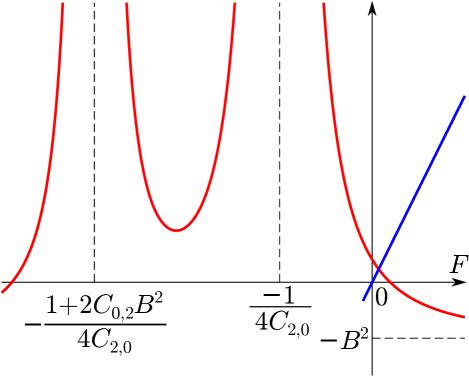
Figure 1: Typical distributions of both sides of Eq. (4) in the case of $D_{1}\neq 0$ and $D_{2}\neq 0$. The red curves are the left-hand side and the blue line is the right-hand side. The vertical axis is the value of each side. The unique intersection expresses the unique solution of $F$. The intersection exists at $F<0$ if $E^{2}<B^{2}$.

IV Examples in one-dimensional cavity

We demonstrate numerical calculations in a one-dimensional cavity system with length $L$ in the $x$ direction, i.e., $0\leq x\leq L$. The mirrors are supposed to be perfect conductors and the boundary conditions are given as the $y,z$ components of the electric field and the $x$ component of the magnetic flux density to be zero. The classical term at $t\geq 0$ is given as the sum of a standing wave and static magnetic flux density:

$$\begin{split}&\boldsymbol{E}_{c}=A\sin\omega t\sin kx\boldsymbol{e}_{y},\\ &\boldsymbol{B}_{c}=A\cos\omega t\cos kx\boldsymbol{e}_{z}+\boldsymbol{B}_{s},\\ \end{split}$$ (7)

where $A$ is the amplitude of the standing wave, the wave number $k$ and frequency $\omega$ are connected to the wave length $\lambda$ via $k=2\pi/\lambda$ and $\omega=ck$, and $\boldsymbol{e}_{y,z}$ are the unit vectors of the $y,z$ directions, respectively. We employ $\lambda=400$ (nm) and $L=100\pi/k$ for numerical calculations. $\boldsymbol{B}_{s}=(0,B_{sy},B_{sz})$ is a constant static magnetic flux density and its magnitude is expressed by $B_{s}$. This external field is highly valuable because it can vary the behavior of the nonlinear correction. For this system and classical term, the $x$ component of all fields are always zero and we do not mention hereinafter. We suppose $(C_{2,0}+C_{0,2})(A^{2}+B_{s}^{2})\ll 1$ because the nonlinear Lagrangian in Eq. (1) is limited to be quartic. The condition of $B^{2}<1/(4C_{2,0})$ always holds for the present calculation. For the given classical term, we calculate the corrective term at $t\geq 0$. The initial values of both corrective electric field and magnetic flux density are set to be zero everywhere because they should be much smaller than $A$.

If $A$ and $B_{s}$ are too small, a huge calculation time is required to see the nonlinear effect beyond the linear approximation. Because of this numerical limitation, we first calculate with unrealistic large parameters. An evaluation for realistic values is performed later in Fig. 4. The amplitude of the standing wave is set to $A=10^{-6}/\sqrt{C_{2,0}}$ and the corresponding intensity $cA^{2}$ is about $1.80\times 10^{22}$ (W/cm²). For the static magnetic flux density, $B_{sy}=10^{-2}/\sqrt{C_{2,0}}$ and $B_{sz}=0$ are used in Fig. 2 and $B_{sy}=B_{sz}=0.5\times 10^{-2}/\sqrt{C_{2,0}}$ are used in Fig. 3. The value $10^{-2}/\sqrt{C_{2,0}}$ corresponds to $10^{-2}\sqrt{\mu_{0}/C_{2,0}}\approx 8.7\times 10^{9}$ (T). While these are too large for experiments in a cavity, the calculation itself is consistent because $(C_{2,0}+C_{0,2})(A^{2}+B_{s}^{2})\ll 1$ holds.

To visualize the nonlinear effect, we define a temporal function that expresses the magnitude of the corrective term throughout the cavity. Let

$$E_{ny}^{(\text{sq})}(t)=\max_{0\leq x\leq L}E_{ny}^{2}(x,t),$$ (8)

and defining $E_{nz}^{(\text{sq})}(t)$, $B_{ny}^{(\text{sq})}(t)$, and $B_{nz}^{(\text{sq})}(t)$ in a similar way, we introduce “the degree of nonlinearity” as

$$\mathsf{N}(t)=\frac{1}{2A}\left[E_{ny}^{(\text{sq})}(t)+E_{nz}^{(\text{sq})}(t)+B_{ny}^{(\text{sq})}(t)+B_{nz}^{(\text{sq})}(t)\right]^{\frac{1}{2}},$$ (9)

to indicate the strength of the nonlinear effect. $\mathsf{N}$ expresses a magnitude ratio of the corrective term to the classical term. For example, if $\mathsf{N}$ is much smaller than unity, a linear approximation will be applicable. On the contrary, when $\mathsf{N}$ is comparable to unity, such an electromagnetic field will not be analyzed by the linear approximation.

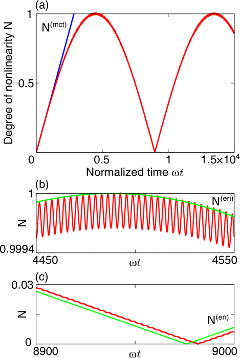
Figure 2: The degree of nonlinearity $\mathsf{N}$ for $A=10^{-6}/\sqrt{C_{2,0}},B_{sy}=10^{-2}/\sqrt{C_{2,0}}$, and $B_{sz}=0$. In (a), $\mathsf{N}^{(\text{mct})}$ is also shown. (b,c) are enlarged graphs at the first peak and zero, respectively. The leading part $\mathsf{N}^{(\text{lp})}$ in Eq. (14) is also shown.

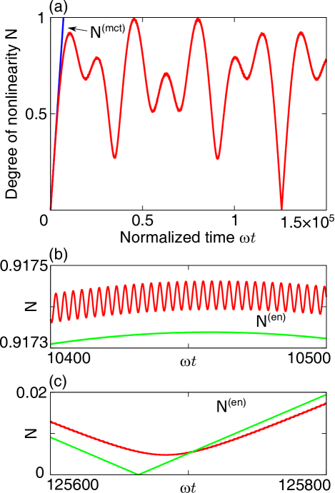
Figure 3: The degree of nonlinearity $\mathsf{N}$ for $A=10^{-6}/\sqrt{C_{2,0}}$ and $B_{sy}=B_{sz}=0.5\times 10^{-2}/\sqrt{C_{2,0}}$. In (a), $\mathsf{N}^{(\text{mct})}$ is also shown. (b,c) are enlarged graphs at the first peak and zero, respectively. The leading part $\mathsf{N}^{(\text{lp})}$ in Eq. (15) is also shown.

We first pay attention to the short time scale. Figures 2(a) and 3(a) show that $\mathsf{N}$ increases almost linearly. In this time scale, the nonlinear correction can be calculated with a linear approximation. The corresponding correction of electromagnetic fields were called as “minimum corrective term” in Ref. [37] and it shows the resonant increase. Let $\mathsf{N}^{(\text{mct})}$ be the degree of nonlinearity for the minimum corrective term. According to Eq. (18) in Ref. [37], $\mathsf{N}^{(\text{mct})}$ behaves almost linear and is consistent with $\mathsf{N}$ in the short time scale, as in Figs. 2(a) and 3(a). As for a longer time scale, the linear approximation becomes an overestimation and $\mathsf{N}$ departs from $\mathsf{N}^{(\text{mct})}$.

Both Figs. 2 and 3 indicate that $\mathsf{N}$ has a slowly varying component as in both panels (a), as well as an oscillation with a period of about $2\pi/\omega$, as in panels (b) and (c). The slower variation is clearly a characteristic of nonlinear electromagnetic waves. In addition, Fig. 3(a) shows more complicated behavior than Fig. 2(a). This may arise from the energy transfer between two polarization modes through $B_{sy}$ and $B_{sz}$.

Readers may wonder how the demonstrated results are related to various previous calculations. The extension of FDTD method is done without making any assumptions except for the form of the Lagrangian. Therefore, it is possible to reproduce the calculation results obtained by a linear approximation or a nonlinear Schrödinger equation. Furthermore, the present scheme is available for the outside of applicable range of these approximations, in particular, in a time scale when the corrective term becomes comparable to the classical term.

V Approximation by leading-part functions

We further inquire into the demonstrated example and reveal a nonlinear characteristic mathematically. The numerical results indicate that the spatial distributions of the electric field are almost always proportional to $\sin kx$ and high-harmonic components are vanishing. These distributions might be attributed to the resonant behavior in the linear approximation: where the resonant increase is proportional to $\omega t\cos\omega t\sin kx$ [37]. We can expect then that the leading part of the electric field will be approximated by a product of a temporal function and $\sin kx$. By expressing by a superscript $(\text{lp})$, the leading part of the electric field and magnetic flux density can be supposed to be

$$\begin{split}&E_{y}^{(\text{lp})}(x,t)=[f\cos\omega t+g\sin\omega t]\sin kx,\\ &E_{z}^{(\text{lp})}(x,t)=(l\cos\omega t+m\sin\omega t)\sin kx,\\ &B_{y}^{(\text{lp})}(x,t)=(-m\cos\omega t+l\sin\omega t)\cos kx+B_{sy},\\ &B_{z}^{(\text{lp})}(x,t)=[g\cos\omega t-f\sin\omega t]\cos kx+B_{sz},\\ \end{split}$$ (10)

where $f,g,l,$ and $m$ depend only on time. They vary relatively slower than $\sin\omega t$ and $\cos\omega t$, i.e., they can be regarded as slowly varying envelopes. They are determined by the following nonlinear differential equations:

$$\begin{pmatrix}f^{\prime}\\ g^{\prime}\\ l^{\prime}\\ m^{\prime}\\ \end{pmatrix}=\begin{pmatrix}0&-\mathscr{X}_{1}-al^{2}&0&-\xi+afl\\ \mathscr{X}_{1}+am^{2}&0&\xi-agm&0\\ 0&-\xi+afl&0&-\mathscr{X}_{2}-af^{2}\\ \xi-agm&0&\mathscr{X}_{2}+ag^{2}&0\\ \end{pmatrix}\begin{pmatrix}f\\ g\\ l\\ m\\ \end{pmatrix},$$ (11)

where

$$\begin{split}&X=f^{2}+g^{2}+l^{2}+m^{2},\\ &\mathscr{X}_{1}=4C_{2,0}B_{sz}^{2}+C_{0,2}B_{sy}^{2}+2C_{2,0}X,\\ &\mathscr{X}_{2}=4C_{2,0}B_{sy}^{2}+C_{0,2}B_{sz}^{2}+2C_{2,0}X,\\ &\xi=-(4C_{2,0}-C_{0,2})B_{sy}B_{sz},\\ &a=-2C_{2,0}+\frac{1}{2}C_{0,2}.\\ \end{split}$$ (12)

A detailed derivation of the differential equations and their solutions are given in Appendix. It can be easily verified that $X=A^{2}$ is a conservative quantity, Note that this fact expresses a physical meaning that a leading part of the total energy conserves in the form of Eq. (10) and the time evolution in Eq. (11).

In this approximation, the corrective term can be approximated as $\boldsymbol{E}_{n}\approx\boldsymbol{E}^{(\text{lp})}-\boldsymbol{E}_{c}$ and $\boldsymbol{B}_{n}\approx\boldsymbol{B}^{(\text{lp})}-\boldsymbol{B}_{c}$. Therefore, the leading part of the degree of nonlinearity $\mathsf{N}^{(\text{lp})}$ can be expressed by

$$\mathsf{N}^{(\text{lp})}(t)=\sqrt{\frac{1}{2}\left(1-\frac{g}{A}\right)}.$$ (13)

We write down the leading part of the total electric field $\boldsymbol{E}^{(\text{lp})}$ and $\mathsf{N}^{(\text{lp})}$ for both Figs. 2 and 3. For Fig. 2, Eq. (A.21) gives

$$\begin{split}&E_{y}^{(\text{lp})}=A\sin(1-\mathscr{X}_{1})\omega t\sin kx,\\ &E_{z}^{(\text{lp})}=0,\\ &\mathsf{N}^{(\text{lp})}(t)=\left|\sin\frac{\mathscr{X}_{1}\omega t}{2}\right|,\\ \end{split}$$ (14)

where $\mathscr{X}_{1}=C_{2,0}(2A^{2}+7B_{s}^{2})$. We can see that $\mathsf{N}^{(\text{lp})}$ becomes zero when $\omega t$ is an integer multiple of $2\pi/\mathscr{X}_{1}\approx 8.976\times 10^{3}$, in accordance with the numerical result as in Fig. 2(c). Equations (A.22) and (A.23) are used for Fig. 3. In the time scale of $C_{2,0}A^{2}\omega t\ll 1$, we obtain

$$\begin{split}&E_{y}^{(\text{lp})}\approx A\cos\xi\omega t\sin(1-11\xi/3)\omega t\sin kx,\\ &E_{z}^{(\text{lp})}\approx-A\sin\xi\omega t\cos(1-11\xi/3)\omega t\sin kx,\\ &\mathsf{N}^{(\text{lp})}(t)\approx\sqrt{\frac{1}{2}\left(1-\cos\xi\omega t\cos\frac{11}{3}\xi\omega t\right)},\\ \end{split}$$ (15)

where $\xi=(3/2)C_{2,0}B_{s}^{2}$. In this case, $\mathsf{N}^{(\text{lp})}$ becomes zero when $\omega t$ is an integer multiple of $2\pi/(C_{2,0}B_{s}^{2})=4\pi\times 10^{4}\approx 1.2566\times 10^{5}$, reproducing the numerical result as in Fig. 3(c).

We can see that $\mathsf{N}^{(\text{lp})}$ does not oscillate rapidly but well reproduces a rough behavior of $\mathsf{N}$: the difference is almost indistinguishable in the scale of panel (a) of both figures. Thus, it is shown only in panels (b) and (c). The slight differences are attributed to the discarded terms in the analytic calculation. Furthermore, $\boldsymbol{E}_{n}$ and $\boldsymbol{B}_{n}$ in a short time scale agree with the resonant increase of the minimum corrective term [37], as calculated in Eq. (A.25). These results confirm the validity of the approximation of leading part in the present time scale. Note that it is not clear that the approximation is valid for an infinitely long time scale.

These results suggest that the nonlinear effect in the one-dimensional cavity appears as changes of the phase and polarization. In contrast, a change in wavelength or frequency must be discrete because of the fixed boundary conditions and high-harmonic components are scarcely generated in the viewpoint of energy conservation.

In the present system, the maximum of $\mathsf{N}$ is about unity. It can be understood from Eq. (13) as it shows $\mathsf{N}^{(\text{lp})}\leq 1$. When $\mathsf{N}^{(\text{lp})}\approx 1$, we can see that $E_{y}^{(\text{lp})}\approx-A\sin\omega t\sin kx$ is necessary, i.e., the whole nonlinear electromagnetic wave is exactly the antiphase to the classical electromagnetic wave, and the phase shift becomes maximum. In Fig. 2, $\mathsf{N}^{(\text{lp})}=1$ is realized when $\omega t$ is an odd integer multiple of $\pi/\mathscr{X}_{1}\approx 4.488\times 10^{3}$, as in Fig. 2(b).

VI Calculation for realistic parameters

The leading-part functions enable us to clarify the behavior of nonlinear electromagnetic waves in much longer time scale than the extended FDTD method can reach. In particular, the leading-part functions are highly useful in the case that the classical amplitude $A$ and the magnitude of the external magnetic flux density $B_{s}$ are relatively small. If we try to run a numerical calculation with the extended FDTD method up to a time scale when the nonlinearity becomes dominant, an unrealistic long calculation time will be required.

We perform a realistic calculation of the classical amplitude to be $1.94\times 10^{6}$ (V/m), corresponding to $10^{6}$ (W/cm²) [40] and the static magnetic flux density to be $5\sqrt{2}$ (T) for both $y$ and $z$ components [41][42]. Because $A$ and $\boldsymbol{B}_{s}$ are realistic, i.e., much smaller than the above values, the leading-part functions will be sufficiently precise approximations.

We demonstrate the time evolution of the polarization. For this purpose, we calculate the intensity ratio of the $y$ component of the electric field to the total electric field and the relative phase. Using Eq. (A.26), the intensity ratio $I_{y}$ is given as

$$I_{y}=\frac{1}{2}[1+\text{cn}(p\omega t,iq)\text{dn}(p\omega t,iq)],$$ (16)

where $p$ and $q$ are given in Eq. (A.17). The relative phase $\Psi_{y-z}$ is defined in Eq. (A.29). Figure 4 shows a result at a fixed point of $\sin kx=1$. Figure 4(a) is a typical time evolution of the polarization mode. It varies between two orthogonal linear polarizations. During the transition, the polarization is almost elliptic because the magnitude and phase of each component of electric field scarcely change in a cycle of $2\pi/\omega$. $I_{y}$ and $\Psi_{y-z}$ are shown in Figs. 4(b) and 4(c), respectively. The value of $I_{y}$, well approximated by $\cos^{2}\xi\omega t$, determines the shape of the ellipse of polarization and the sign of $\Psi_{y-z}$ determines the rotation direction. In particular, the polarization changes by 90 degrees from $y$ to $z$ at $t\approx\pi/(2\xi\omega)=\pi/(3C_{2,0}B_{s}^{2}\omega)\approx 1.68\times 10^{6}$ seconds.

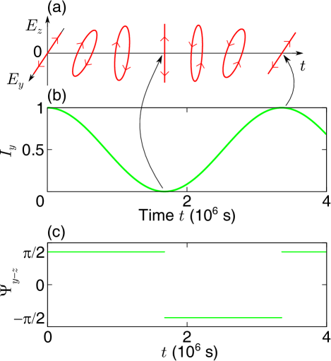
Figure 4: The time evolution of the polarization at a position of $\sin kx=1$. (a) The shapes and rotation directions of the elliptical polarization. The axes of ellipses are almost coincident with the $y$ and $z$ axes. (b) The intensity ratio $I_{y}$ in Eq. (16). (c) The relative phase $\Psi_{y-z}$ in Eq. (A.29). Its sign determines the rotation direction.

We briefly discuss an experimental perspective for the demonstrated example. Suppose we connect the ratio $I_{y}$ and a detectable polarization angle $\theta$ (deg) of precise measurement, we can estimate a necessary time to confine the standing wave in the cavity by $\cos^{2}\xi\omega t\approx\cos(\theta\pi/180)$, yielding

$$t\approx\frac{\mu_{0}\lambda}{3\pi cC_{2,0}B_{s}^{2}}\text{Cos}^{-1}\sqrt{\cos\frac{\theta}{180}\pi}.$$ (17)

If we take $\theta=0.003$ [43] and $B_{sy}=B_{sz}=30$ (T) [44], the necessary time is $t\approx 2.20$ seconds. On the other hand, even if a high reflectivity mirror is employed such as in gravitational wave detectors [45][46] [47], a light in the cavity vanishes within several milliseconds for a cavity length of $L=30$ (cm). There is a gap of time scales by 3-digits. To bridge the gap or to find other features of self-modulation may be important open problems for future verification experiments. For example, to decrease the loss by reflection, a longer cavity with partial external fields or compensation by a successive adequate input will be reasonable. The extension of FDTD method is also useful for such calculations. In addition, realistic boundary conditions will be necessary for a high reflectivity mirror with a multilayer stack [47][48].

VII Final remarks

We have extended the FDTD method to execute a numerical calculation without making any assumptions except for the form of the nonlinear Lagrangian to be quartic. We demonstrated the nonlinear electromagnetic waves in a one-dimensional cavity. We further derived an analytic approximation as the leading-part functions and mathematically clarified a characteristic of the nonlinear standing waves. The numerical and analytical results in a one-dimensional cavity are not simply as same as the well-known birefringence. In a calculation of the birefringence, a propagating wave in a cavity is frequently assumed to be sufficiently smaller than an external field and to be a plane-wave eigenmode, resulting in the time-independent dispersion relation [25][27] [49][50]. Several studies show a time-dependent dispersion relation by using a perturbation [27][51]. The present calculations are performed without these assumptions. For example, the propagating wave does not have to be smaller than the external field, in particular, the phase can self-modulate without external field. We have not considered a dispersion relation because it is not adequate to approximate a nonlinear electromagnetic wave in a cavity by a plane wave.

The extended FDTD method is applicable to even more general systems, i.e., not limited to a cavity system, and may reproduce numerous previous results obtained by a linear approximation or a nonlinear Schrödinger equation. For example, if the time scale of nonlinear interaction is extremely short, such as a focusing of high power lasers, calculation results of the extended FDTD method and the linear approximation will be in good agreement. The most important physical picture of the present study is that a momentarily small nonlinear effect can accumulate and can appear as a comparably large self-modulation in a long time scale, even though the input or classical electromagnetic field is small. Such a novel property is not calculated if the corrective term is assumed to be always sufficiently smaller than the classical term. While, the larger electromagnetic fields are preferable because the nonlinear effect can appear in shorter time. The extended FDTD method will enable us to discover novel properties of nonlinear electromagnetic waves in a time scale when the nonlinearity becomes dominant, yielding new and optimized verification experiments of nonlinear electromagnetism in vacuum.

*

.1 Appendix: Calculation of the leading-part functions

In this appendix, we explain a detailed analysis of the leading-part functions in Eq. (10). The derivation of the differential equations in Eq. (11) and their solutions are shown. Originally, the leading-part functions of the electric field and magnetic flux density are introduced as

$$\begin{split}&E_{y}^{(\text{lp})}(x,t)=[f\cos\omega t+(g-A)\sin\omega t]\sin kx,\\ &E_{z}^{(\text{lp})}(x,t)=(l\cos\omega t+m\sin\omega t)\sin kx,\\ &B_{y}^{(\text{lp})}(x,t)=(-\tilde{m}\cos\omega t+\tilde{l}\sin\omega t)\cos kx+B_{sy},\\ &B_{z}^{(\text{lp})}(x,t)=[(\tilde{g}-A)\cos\omega t-\tilde{f}\sin\omega t]\cos kx+B_{sz}.\\ \end{split}$$ (A.1 )

In the following calculations, $T=\omega t$ is used as a new variable. All the functions of $f,g,l,m$, and tilde-added ones depend only on $T$ and supposed to vary slower than $\sin T$ and $\cos T$. They are determined by the nonlinear Maxwell’s equations given as

$$\begin{split}&-\frac{\partial}{\partial x}E_{z}^{(\text{lp})}+c^{-1}\frac{\partial}{\partial t}B_{y}^{(\text{lp})}=0,\\ &\frac{\partial}{\partial x}E_{y}^{(\text{lp})}+c^{-1}\frac{\partial}{\partial t}B_{z}^{(\text{lp})}=0,\\ &-\frac{\partial}{\partial x}H_{z}^{(\text{lp})}-c^{-1}\frac{\partial}{\partial t}D_{y}^{(\text{lp})}=0,\\ &\frac{\partial}{\partial x}H_{y}^{(\text{lp})}-c^{-1}\frac{\partial}{\partial t}D_{z}^{(\text{lp})}=0.\\ \end{split}$$ (A.2 )

.1.1 1st and 2nd lines of Maxwell’s equations

The first line of the Maxwell’s equations gives

$$(l-\tilde{l}+\tilde{m}^{\prime})\cos T+(m-\tilde{m}-\tilde{l}^{\prime})\sin T=0.$$ (A.3 )

Each parenthesis varies slowly and is supposed to be zero, i.e.,

$$l-\tilde{l}+\tilde{m}^{\prime}=0,\ \ m-\tilde{m}-\tilde{l}^{\prime}=0.$$ (A.4 )

Similarly, the second line gives

$$(f-\tilde{f}+\tilde{g}^{\prime})\cos T+(g-\tilde{g}-\tilde{f}^{\prime})\sin T=0,$$ (A.5 )

yielding

$$f-\tilde{f}+\tilde{g}^{\prime}=0,\ \ g-\tilde{g}-\tilde{f}^{\prime}=0.$$ (A.6 )

Because $f$ and the other functions vary relatively slowly, their derivatives will be comparably small if they are not identically zero. Combining with above suppositions, it will be adequate to suppose the following:

$$\begin{split}&f\approx\tilde{f},\ \ g\approx\tilde{g},\ \ l\approx\tilde{l},\ \ m\approx\tilde{m},\\ &f^{\prime}\approx\tilde{f}^{\prime},\ \ g^{\prime}\approx\tilde{g}^{\prime},\ \ l^{\prime}\approx\tilde{l}^{\prime},\ \ m^{\prime}\approx\tilde{m}^{\prime}.\\ \end{split}$$ (A.7 )

Equations (A.4), (A.6), and (A.7) enable us to approximate as

$$\begin{split}&\tilde{f}=f+g^{\prime},\\ &\tilde{g}=g-f^{\prime},\\ &\tilde{l}=l+m^{\prime},\\ &\tilde{m}=m-l^{\prime},\\ \end{split}$$ (A.8 )

and we erase the four tilde-added functions from our calculation. In addition, the tilde-added functions are replaced in Eq. (10) in the main text.

.1.2 3rd and 4th lines of Maxwell’s equations

Substituting the classical and corrective terms into the third and fourth lines of the Maxwell’s equations shows a dependence on $x$ by $\sin kx$ and $\sin 3kx$. We only retain the part of $\sin kx$. For the temporal part, the terms which oscillate faster than $\cos T$ and $\sin T$ are discarded, such as $\sin 2T$. Finally, the terms multiplied by $\cos T$ and $\sin T$ are regarded as zero independently, as in the above postulates, we obtain four differential equations on the slowly varying functions. Each of $f,g,l$, and $m$ is expected to be at most of the order of $A$. The products of a nonlinear parameter and two functions such as $C_{2,0}fl$ will be much smaller than unity. Therefore, the product of such values and the derivatives are excluded. Finally, the simultaneous differential equations in Eq. (11) are derived.

.2 Solution

We solve the equations in Eq. (11) given the initial conditions of $f(0)=0,g(0)=A,l(0)=0$, and $m(0)=0$. First, we can see $X^{\prime}=0$. Therefore, $X=A^{2}$ is constant and $\mathscr{X}_{1}$ and $\mathscr{X}_{2}$ are also constant. In particular, all of $f,g,l$, and $m$ are bounded and at most of the order of $A$. We introduce three variables by

$$\alpha=f^{2}+g^{2},\ \ \beta=fl+gm,\ \ \gamma=-fm+gl.$$ (A.9 )

Defining a new constant as

$$\Delta=\mathscr{X}_{1}-\mathscr{X}_{2},$$ (A.10 )

we obtain differential equations for $\alpha,\beta$, and $\gamma$ as

$$\begin{split}&\alpha^{\prime}=2\gamma(\xi-a\beta),\\ &\beta^{\prime}=\gamma[-\Delta+a(2\alpha-X)],\\ &\gamma^{\prime}=\Delta\beta+\xi(X-2\alpha),\\ \end{split}$$ (A.11 )

with the initial conditions of $\alpha(0)=A^{2},\beta(0)=0$, and $\gamma(0)=0$ . Because $f^{2}+g^{2}+l^{2}+m^{2}=A^{2}$, the range of $\alpha,\beta$, and $\gamma$ are bounded. Hence, the set of differential equations is Lipschitz continuous and the solution for the initial value problem is unique.

We first calculate for $\xi\neq 0$. Let

$$Z=\Delta(-\Delta+aX)-4\xi^{2},$$ (A.12 )

and also

$$p=\sqrt{\frac{-Z+\sqrt{Z^{2}+4\xi^{2}a^{2}X^{2}}}{2}},\ \ q=\frac{-\xi aX}{p^{2}},$$ (A.13 )

we obtain

$$\begin{split}&\alpha=\frac{X}{4\xi^{2}+\Delta^{2}}\left\{\Delta^{2}+\Delta\xi q\text{sn}^{2}(pT,iq)+2\xi^{2}\left[1+\text{cn}(pT,iq)\text{dn}(pT,iq)\right]\right\},\\ &\beta=\frac{\xi X}{4\xi^{2}+\Delta^{2}}\left\{2\xi q\text{sn}^{2}(pT,iq)+\Delta\left[1-\text{cn}(pT,iq)\text{dn}(pT,iq)\right]\right\},\\ &\gamma=-\frac{\xi X}{p}\text{sn}(pT,iq).\\ \end{split}$$ (A.14 )

We give $f,g,l$, and $m$ for individual cases. In any case, their derivatives are sufficiently smaller than the maximum value of the original function and consistent with the discussion and assumptions around Eq. (A.7).

.2.1 $f,g,l$, and $m$ for $\xi\neq 0$ and $\Delta\neq 0$

The case of $\xi\neq 0$, and $\Delta\neq 0$ corresponds to $B_{sy}\neq 0,B_{sz}\neq 0$, and $B_{sy}\neq B_{sz}$. In this case, $\alpha>0$ always holds and $\sqrt{\alpha}$ is always differentiable. Therefore, let

$$\Theta=\mathscr{X}_{1}T+\int_{0}^{T}\frac{\xi\beta(\tau)+a\gamma(\tau)^{2}}{\alpha(\tau)}\text{d}\tau,$$ (A.15 )

we obtain

$$\begin{split}&f=-\sqrt{\alpha}\sin\Theta,\\ &g=\sqrt{\alpha}\cos\Theta,\\ &l=\frac{1}{\sqrt{\alpha}}(-\beta\sin\Theta+\gamma\cos\Theta),\\ &m=\frac{1}{\sqrt{\alpha}}(\beta\cos\Theta+\gamma\sin\Theta).\\ \end{split}$$ (A.16 )

.2.2 $f,g,l$, and $m$ for $\xi\neq 0$ and $\Delta=0$

The case of $\xi\neq 0$ and $\Delta=0$ corresponds to $|B_{sy}|=|B_{sz}|\neq 0$. In this case,

$$p=\sqrt{2\xi^{2}+|\xi|\sqrt{4\xi^{2}+a^{2}X^{2}}},\ \ q=\frac{-\text{sgn}(\xi)aX}{2|\xi|+\sqrt{4\xi^{2}+a^{2}X^{2}}},$$ (A.17 )

and in particular, $|q|<1$. The double-angle formula of Jacobi elliptic function yields

$$\frac{\alpha}{X}=\frac{1}{2}[1+\text{cn}(pT,iq)\text{dn}(pT,iq)]=\frac{\text{cn}^{2}(pT/2,iq)\text{dn}^{2}(pT/2,iq)[1-q^{2}\text{sn}^{4}(pT/2,iq)]}{[1+q^{2}\text{sn}^{4}(pT/2,iq)]^{2}}.$$ (A.18 )

Because $|q|<1$, $\alpha=0$ holds if and only if $\text{cn}(pT/2,iq)=0$. Then, using

$$\Theta=\mathscr{X}_{1}T-q\xi\int_{0}^{T}\frac{\text{sn}(p\tau,iq)^{2}}{1+\text{cn}(p\tau,iq)\text{dn}(p\tau,iq)}\text{d}\tau,$$ (A.19 )

we obtain

$$\begin{split}&f=-A\frac{\text{cn}(pT/2,iq)\text{dn}(pT/2,iq)\sqrt{1-q^{2}\text{sn}^{4}(pT/2,iq)}}{1+q^{2}\text{sn}^{4}(pT/2,iq)}\sin\Theta,\\ &g=A\frac{\text{cn}(pT/2,iq)\text{dn}(pT/2,iq)\sqrt{1-q^{2}\text{sn}^{4}(pT/2,iq)}}{1+q^{2}\text{sn}^{4}(pT/2,iq)}\cos\Theta,\\ &l=-\frac{2A\xi\text{sn}(pT/2,iq)}{p\sqrt{1-q^{2}\text{sn}^{4}(pT/2,iq)}}\left[-\frac{aX}{2p}\text{sn}(pT,iq)\sin\Theta+\cos\Theta\right],\\ &m=-\frac{2A\xi\text{sn}(pT/2,iq)}{p\sqrt{1-q^{2}\text{sn}^{4}(pT/2,iq)}}\left[\frac{aX}{2p}\text{sn}(pT,iq)\cos\Theta+\sin\Theta\right].\\ \end{split}$$ (A.20 )

.2.3 $f,g,l$, and $m$ for $\xi=0$

This case corresponds to $B_{sy}=0$ or $B_{sz}=0$. We immediately see $\alpha=A^{2},\beta=0,\gamma=0$, and obtain

$$\begin{split}&f=-A\sin\mathscr{X}_{1}T,\\ &g=A\cos\mathscr{X}_{1}T,\\ &l=0,\\ &m=0.\\ \end{split}$$ (A.21 )

The result contains the case of $\Delta=0$, i.e., $B_{s}=0$.

.2.4 Approximation for $A\ll|B_{sy}|=|B_{sz}|$

In the case of $A\ll|B_{sy}|=|B_{sz}|$, the solution given in Eqs. (A.19) and (A.20) can be approximated in a simple form. $p\approx 2|\xi|$ and $q\approx 0$ hold because $aX\ll|\xi|$. Therefore,

$$\begin{split}&f\approx-A\cos\xi T\sin\Theta,\\ &g\approx A\cos\xi T\cos\Theta,\\ &l\approx-A\sin\xi T\cos\Theta,\\ &m\approx-A\sin\xi T\sin\Theta,\\ \end{split}$$ (A.22 )

where

$$\Theta\approx\left(\mathscr{X}_{1}+\frac{aX}{4}\right)T-\frac{aX}{8\xi}\sin 2\xi T\approx\left(\mathscr{X}_{1}+\frac{aX}{4}\right)T.$$ (A.23 )

The oscillating term can be discarded because its absolute value is much smaller than unity.

.3 Comparison to minimum corrective term

We calculate for a short time scale. All of Eqs. (A.16), (A.20), and (A.21) express $f,g,l$, and $m$ give

$$\begin{split}&f=-A\mathscr{X}_{1}T+O(T^{2}),\\ &g=A+O(T^{2}),\\ &l=-A\xi T+O(T^{2}),\\ &m=O(T^{2}).\\ \end{split}$$ (A.24 )

Therefore, the main part of the corrective term in the short time scale are

$$\begin{split}&E_{ny}\approx-A\mathscr{X}_{1}\omega t\cos\omega t\sin kx,\\ &E_{nz}\approx-A\xi\omega t\cos\omega t\sin kx,\\ &B_{ny}\approx-A\xi\omega t\sin\omega t\cos kx,\\ &B_{nz}\approx A\mathscr{X}_{1}\omega t\sin\omega t\cos kx.\\ \end{split}$$ (A.25 )

.4 Calculation of the polarization

For the calculation for Fig. 4 using realistic parameters, we derive the intensity ratio of the $y$ component to the entire electric field $I_{y}$ and the relative phase $\Psi_{y-z}$.

Each amplitude of the $y$ and $z$ component is given by $\sqrt{f^{2}+g^{2}}$ and $\sqrt{l^{2}+m^{2}}$, respectively, and the ratio $I_{y}$ is given by

$$I_{y}=\frac{f^{2}+g^{2}}{f^{2}+g^{2}+l^{2}+m^{2}}=\frac{\alpha}{A^{2}}=\frac{1}{2}[1+\text{cn}(pT,iq)\text{dn}(pT,iq)].$$ (A.26 )

As for the relative phase, Eq. (A.20) for $f,g,l$, and $m$ and Eq. (A.19) for $\Theta$ yield

$$\begin{split}&E_{y}^{(\text{lp})}(x,t)=A\sqrt{\frac{1+\text{cn}(pT,iq)\text{dn}(pT,iq)}{2}}\sin(T-\Theta+\theta_{c})\sin kx,\\ &E_{z}^{(\text{lp})}(x,t)=A\sqrt{\frac{1-\text{cn}(pT,iq)\text{dn}(pT,iq)}{2}}\sin(T-\Theta-\Psi_{0}+\theta_{s})\sin kx,\\ \end{split}$$ (A.27 )

where the phase factors $\Psi_{0}\in(0,\pi)$, $\theta_{c}$, and $\theta_{s}$ are defined as

$$\begin{split}&\sin\Psi_{0}=\frac{1}{\sqrt{1+[aX\text{sn}(pT,iq)/(2p)]^{2}}},\ \ \cos\Psi_{0}=-\frac{aX\text{sn}(pT,iq)/(2p)}{\sqrt{1+[aX\text{sn}(pT,iq)/(2p)]^{2}}},\\ &\theta_{c}=\begin{cases}0&\boldsymbol{(}\text{cn}(pT/2,iq)\geq 0\boldsymbol{)}\\ \pi&\boldsymbol{(}\text{cn}(pT/2,iq)<0\boldsymbol{)}\\ \end{cases},\\ &\theta_{s}=\begin{cases}0&\boldsymbol{(}\text{sn}(pT/2,iq)\geq 0\boldsymbol{)}\\ \pi&\boldsymbol{(}\text{sn}(pT/2,iq)<0\boldsymbol{)}\\ \end{cases}.\\ \end{split}$$ (A.28 )

The phases of both components $\Psi_{y}$ and $\Psi_{z}$ can be defined as $\Psi_{y}=-\Theta+\theta_{c}$ and $\Psi_{z}=-\Theta-\Psi_{0}+\theta_{s}$, respectively. Then, the relative phase can be defined by

$$\Psi_{y-z}=\Psi_{0}-\theta_{cs},$$ (A.29 )

where

$$\theta_{cs}=\begin{cases}0&\boldsymbol{(}\text{sn}(pT/2,iq)\text{cn}(pT/2,iq)\geq 0\boldsymbol{)}\\ \pi&\boldsymbol{(}\text{sn}(pT/2,iq)\text{cn}(pT/2,iq)<0\boldsymbol{)}\\ \end{cases}.$$ (A.30 )

We have defined $\Psi_{y-z}$ and $\theta_{cs}$ as above so that $\Psi_{y-z}$ ranges in $-\pi<\Psi_{y-z}<\pi$. The sign of $\Psi_{y-z}$ changes before and after at a time when $\text{sn}(pT/2,iq)=0$ or $\text{cn}(pT/2,iq)=0$ holds.