Schrödinger-Föllmer Sampler: Sampling without Ergodicity

Abstract

Sampling from probability distributions is an important problem in statistics and machine learning, specially in Bayesian inference when integration with respect to posterior distribution is intractable and sampling from the posterior is the only viable option for inference. In this paper, we propose Schrödinger-Föllmer sampler (SFS), a novel approach to sampling from possibly unnormalized distributions. The proposed SFS is based on the Schrödinger-Föllmer diffusion process on the unit interval with a time-dependent drift term, which transports the degenerate distribution at time zero to the target distribution at time one. Compared with the existing Markov chain Monte Carlo samplers that require ergodicity, SFS does not need to have the property of ergodicity. Computationally, SFS can be easily implemented using the Euler-Maruyama discretization. In theoretical analysis, we establish non-asymptotic error bounds for the sampling distribution of SFS in the Wasserstein distance under reasonable conditions. We conduct numerical experiments to evaluate the performance of SFS and demonstrate that it is able to generate samples with better quality than several existing methods.

KEY WORDS: Euler-Maruyama discretization, Non-asymptotic error bound, Schrödinger bridge, Unnormalized distribution, Wasserstein distance.

1 Introduction

Sampling from a probability distribution is a fundamental problem in statistics and machine learning. For example, the ability to efficiently sample from an unnormalized posterior distribution is crucial to the success of Bayesian inference. Many sampling approaches have been developed in the literature. In particular, there is a large body of work on the Markov Chain Monte Carlo (MCMC) methods, including the celebrated Metropolis-Hastings (MH) algorithm (Metropolis et al.,, 1953; Hastings,, 1970; Tierney,, 1994), the Gibbs sampler (Geman and Geman,, 1984; Gelfand and Smith,, 1990), the Langevin algorithm (Roberts et al.,, 1996; Dalalyan, 2017b, ; Durmus et al.,, 2017), the bouncy particle sampler (Peters et al.,, 2012; Bouchard-Côté et al.,, 2018), and the zig-zag sampler (Bierkens et al.,, 2019), among others, see (Martin et al.,, 2020; Changye and Robert,, 2020; Dunson and Johndrow,, 2020; Brooks et al.,, 2011) and the references therein.

Among these methods, the Langevin sampler based on the Euler-Maruyama discretization of Langevin diffusion has received much attention recently. The Langevin diffusion reads

$$dL_{t}=-\nabla V(L_{t})dt+\sqrt{2}\,dB_{t},$$ (1.1)

where $-\nabla V(\cdot)$ is the drift term and $\{B_{t}\}_{t\geq 0}$ is a standard $p$-dimensional Brownian motion process. Under suitable conditions, the Langevin diffusion process $\{L_{t}\}_{t\geq 0}$ in (1.1) admits an invariant distribution $\mu(x)=\exp(-V(x))/C,x\in\mathbb{R}^{p}$ with normalizing constant $C>0$ (Bakry et al.,, 2008; Cattiaux and Guillin,, 2009). Nice convergence properties of the Langevin sampler under the strongly convex potential assumption have been established by several authors (Durmus et al.,, 2019; Durmus and Moulines,, 2016; Dalalyan, 2017a, ; Dalalyan, 2017b, ; Cheng and Bartlett,, 2018; Dalalyan and Karagulyan,, 2019). Furthermore, the strongly convex potential assumption can be replaced by different conditions to guarantee the log-Sobolev inequality for the target distribution, including the dissipativity condition for the drift term (Raginsky et al.,, 2017; Mou et al.,, 2019; Zhang et al., 2019b, ) and the local convexity condition for the potential function outside a ball (Durmus et al.,, 2017; Cheng et al.,, 2018; Ma et al.,, 2019; Bou-Rabee et al.,, 2020).

Although tremendous progress has been made in the past decades, it remains a challenging task to sample from distributions with multiple modes or distributions in high dimensions (Dunson and Johndrow,, 2020). Even for the one-dimensional Gaussian mixture model $0.5N(-1,\sigma^{2})+0.5N(1,\sigma^{2})$, the optimally tuned Hamiltonian Monte Carlo and the random walk Metropolis algorithms have the mixing time proportional to $\exp({1}/{(2\sigma^{2})})$ (Mangoubi et al.,, 2018; Dunson and Johndrow,, 2020), which will blow up exponentially as $\sigma$ decreases to $0$. The constant in the log-Sobolev inequality may depend on the dimensionality exponentially (Menz et al.,, 2014; Wang et al.,, 2009; Hale,, 2010; Raginsky et al.,, 2017), indicating that the efficiency of Langevin sampler may suffer from the curse of dimensionality when the ambient dimension $p$ is high.

In this paper, we propose Schrödinger-Föllmer sampler (SFS), a novel sampling approach without requiring the property of ergodicity. SFS is based on the Schrödinger-Föllmer diffusion

$$\mathrm{d}X_{t}=b(X_{t},t)\mathrm{d}t+\mathrm{d}B_{t},\ X_{0}=0,\ t\in[0,1],$$ (1.2)

where the function $b:\mathbb{R}^{p}\times[0,1]\to\mathbb{R}^{p}$ is a time-varying drift term determined by the target distribution. The specific form of $b$ is given by (2.8) below. According to Léonard, (2014) and Eldan et al., (2020), the process $\{X_{t}\}_{t\in[0,1]}$ (1.2) was first formulated by Föllmer (Föllmer,, 1985, 1986, 1988) when studying the Schrödinger bridge problem (Schrödinger,, 1932).

The law of $\{X_{t}\}_{t\in[0,1]}$ in (1.2) minimizes the relative entropy with respect to the Wiener measure among all processes with laws interpolating $\delta_{0}$ (the degenerate distribution at $X_{0}=0$) and the target distribution $\mu$ (Jamison,, 1975; Dai Pra,, 1991; Léonard,, 2014). Therefore, the diffusion process (1.2) can be used to sample from the target distribution $\mu$ by transporting the initial degenerate distribution at $t=0$ to the target $\mu$ at $t=1$. To numerically implement this sampling approach, we use the Euler-Maruyama method to discretize the diffusion process (1.2). The resulting discretized version of (1.2) is

$$Y_{t_{k+1}}=Y_{t_{k}}+\delta_{k}b\left(Y_{t_{k}},t_{k}\right)+\sqrt{\delta_{k}}\epsilon_{k+1},\ k=0,1,\ldots,K-1,\ K\geq 2,$$ (1.3)

where $K$ is the number of the grid points on $[0,1]$ with $0=t_{0}<t_{1}<\ldots<t_{K}=1$, $\delta_{k}=t_{k+1}-t_{k}$ is the $k$-th step size, and $\{\epsilon_{k}\}_{k=1}^{K}$ are independent and identically distributed random vectors from $N(0,\mathbf{I}_{p})$. Based on (1.3), we can start from $Y_{t_{0}}=0$ and iteratively update this initial value to obtain a realization of the random vector $Y_{t_{K}}$, which is approximately distributed as the target distribution $\mu$ under suitable conditions. For convenience, we shall refer to the proposed sampling method as the Schrödinger-Föllmer sampler (SFS).

An important difference between SFS and existing MCMC methods is that ergodicity is not required for SFS to generate valid samples. This is due to the basic property of the Schrödinger-Föllmer diffusion (1.2) on the unit time interval $[0,1]$, which transports the initial distribution $\delta_{0}$ at $t=0$ to the exact target distribution $\mu$ at $t=1$. The sampling error of SFS is entirely due to the Euler-Maruyama discretization and the approximation of the drift term in the Schrödinger-Föllmer diffusion. These two type of approximation errors can be made arbitrarily small under suitable conditions.

Our main contributions are as follows.

1. We propose a novel sampling method SFS without assuming ergodicity. SFS is based on Euler-Maruyama discretization to the Schrödinger-Föllmer diffusion. The proposed SFS also works for unnormalized distributions.

2. We establish non-asymptotic bounds for the difference between the law of the samples generated via SFS and the target distribution $\mu$ in terms of the Wasserstein distance under appropriate conditions. When the drift term $b$ can be calculated in a closed form, for example the target $\mu$ is a finite mixture of Gaussians, we show that

   $$W_{2}(\mbox{Law}(Y_{t_{K}}),\mu)\leq\mathcal{O}(\sqrt{p/K})$$

   under some smoothness conditions on the drift term, see Theorem 4.1. In the case when the drift term needs to be calculated via Monte Carlo approximation, we prove that

   $$W_{2}(\mbox{Law}(\widetilde{Y}_{t_{K}}),\mu)\leq\mathcal{O}(\sqrt{p}(1/\sqrt{K}+1/\sqrt{m}))$$

   under the assumption that the potential $U(x,t)$ in (2.7) below is strongly convex with respect to $x$, where $m$ is the number of Gaussian samples used in the Monte Carlo approximation of $b$, see Theorem 4.3.

3. We conduct numerical experiments to evaluate the effectiveness of the proposed SFS and demonstrate that SFS performs better than several existing MCMC methods for Gaussian mixture models and Bayesian logistic regression.

The rest of the paper is organized as follows. In Section 2 we recall some background and present the proposed SFS in details. In Section 3 we compare SFS with Langevin sampler when the target distribution is a standard normal distribution. In Section 4 we establish the non-asymptotic bounds on the Wasserstein distance between the distribution of the samples generated via SFS and the target one. In Section 6 we conduct simulation studies to assess the performance of SFS. Concluding remarks are given in Section 7. Proofs for all the theorems are provided in Appendix A.

We end this section by introducing some notation used throughout the paper. Denote $\mathcal{B}(\mathbb{R}^{p})$ as the Borel set of $\mathbb{R}^{p}$, and let $\mathcal{P}\left(\mathbb{R}^{p}\right)$ be the collection of probability measures on $(\mathbb{R}^{p},\mathcal{B}(\mathbb{R}^{p}))$. Denote the gradient of a smooth function $\varphi(x),x\in\mathbb{R}^{p}$ by $\nabla\varphi(x)$. Similarly, denote the partial derivative with respect to $x$ of $\phi(x,t),(x,t)\in\mathbb{R}^{p}\times[0,1]$ by $\nabla_{x}\phi(x,t)$. For symmetric matrices ${\bf A},{\bf B}\in\mathbb{R}^{p\times p}$, ${\bf A}>{\bf B}$ means that ${\bf A}-{\bf B}$ is a positive definite matrix. Let $\|\beta\|_{\ell}=(\sum_{i=1}^{p}|\beta_{i}|^{\ell})^{\frac{1}{\ell}}$ be the $\ell$-norm of the vector $\beta=(\beta_{1},\ldots,\beta_{p})^{\top}\in\mathbb{R}^{p}$. Denote $\|X\|_{L_{2}}=(\mathbb{E}\|X\|_{2}^{2})^{1/2}$ as the $L_{2}$-norm of a random vector $X$. Denote $\mathbb{E}_{X}$ as the expectation over the random vector $X$.

2 Schrödinger-Föllmer sampler

In this section we first provide some background on the Schrödinger-Föllmer diffusion. We then present the proposed SFS method based on the Euler-Maruyama discretization of the Schrödinger-Föllmer diffusion.

2.1 Background on Schrödinger-Föllmer diffusion

We first recall the Schrödinger bridge problem, then introduce the Schrödinger-Föllmer diffusion, and at last calculate the closed form expression of the drift term in the scenario that the target distribution is a Gaussian mixture.

2.1.1 Schrödinger bridge problem

Let $\Omega=C([0,1],\mathbb{R}^{p})$ be the space of $\mathbb{R}^{p}$-valued continuous functions on the time interval $[0,1]$. Denote $Z=(Z_{t})_{t\in[0,1]}$ as the canonical process on $\Omega$, where $Z_{t}(\omega)=\omega_{t}$, $\omega=(\omega_{s})_{s\in[0,1]}\in\Omega$. The canonical $\sigma$-field on $\Omega$ is then generated as $\mathscr{F}=\sigma(Z_{t},t\in[0,1])=\left\{\{\omega:(Z_{t}(\omega))_{t\in[0,1]}\in H\}:H\in\mathcal{B}(\mathbb{R}^{p})\right\}$. Denote $\mathcal{P}(\Omega)$ as the space of probability measures on the path space $\Omega$, and $\mathbf{W}_{\mathbf{x}}\in\mathcal{P}(\Omega)$ as the Wiener measure whose initial marginal is $\delta_{\mathbf{x}}$. The law of the reversible Brownian motion, is then defined as $\mathbf{P}=\int\mathbf{W}_{\mathbf{x}}\mathrm{d}\mathbf{x}$, which is an unbounded measure on $\Omega$. One can observe that, $\mathbf{P}$ has a marginal coinciding with the Lebesgue measure $\mathscr{L}$ at each $t$. Schrödinger, (1932) studied the problem of finding the most likely random evolution between two probability distributions $\widetilde{\nu},\widetilde{\mu}\in\mathcal{P}(\mathbb{R}^{p})$. This problem is referred to as the Schrödinger bridge problem (SBP). SBP can be further formulated as seeking a probability law on the path space that interpolates between $\widetilde{\nu}$ and $\widetilde{\mu}$, such that the probability law is close to the prior law of the Brownian diffusion with respect to the relative entropy (Jamison,, 1975; Léonard,, 2014), i.e., finding a path measure $\mathbf{Q}^{*}\in\mathcal{P}(\Omega)$ with marginal $\mathbf{Q}^{*}_{t}=(Z_{t})_{\#}\mathbf{Q}^{*}=\mathbf{Q}^{*}\circ Z_{t}^{-1},t\in[0,1]$ such that

$$\mathbf{Q}^{*}\in\arg\min\mathbb{D}_{\mathrm{KL}}(\mathbf{Q}||\mathbf{P}),$$

and

$$\mathbf{Q}_{0}=\widetilde{\nu},\mathbf{Q}_{1}=\widetilde{\mu},$$

where the relative entropy $\mathbb{D}_{\mathrm{KL}}(\mathbf{Q}||\mathbf{P})=\int\log(\frac{d\mathbf{Q}}{d\mathbf{P}})d\mathbf{Q}$ if $\mathbf{Q}\ll\mathbf{P}$ (i.e. $\mathbf{Q}$ is absolutely continuous w.r.t. $\mathbf{P}$), and $\mathbb{D}_{\mathrm{KL}}(\mathbf{Q}||\mathbf{P})=\infty$ otherwise. The following theorem characterizes the solution of SBP.

Theorem 2.1.

(Léonard,, 2014) If $\widetilde{\nu},\widetilde{\mu}\ll\mathscr{L}$, then SBP admits a unique solution $\mathbf{Q}^{*}=f^{*}(Z_{0})g^{*}(Z_{1})\mathbf{P}$, where $f^{*}$ and $g^{*}$ are $\mathscr{L}$-measurable nonnegative functions satisfying the Schrödinger system

$$\left\{\begin{array}[]{l}f^{*}(\mathbf{x})\mathbb{E}_{\mathbf{P}}\left[g^{*}\left(Z_{1}\right)\mid Z_{0}=\mathbf{x}\right]=\frac{d\widetilde{\nu}}{d\mathscr{L}}(\mathbf{x}),\quad\mathscr{L}-a.e.\\ g^{*}(\mathbf{y})\mathbb{E}_{\mathbf{P}}\left[f^{*}\left(Z_{0}\right)\mid Z_{1}=\mathbf{y}\right]=\frac{d\widetilde{\mu}}{d\mathscr{L}}(\mathbf{y}),\quad\mathscr{L}-a.e.\end{array}\right.$$

Furthermore, the pair $(\mathbf{Q}^{*}_{t},\mathbf{v}^{*}_{t})$ with

$$\mathbf{v}^{*}_{t}(\mathbf{x})=\nabla_{\mathbf{x}}\log\mathbb{E}_{\mathbf{P}}\left[g^{*}\left(Z_{1}\right)\mid Z_{t}=\mathbf{x}\right]$$

solves the minimum action problem

$$\min_{\mu_{t},\mathbf{v}_{t}}\int_{0}^{1}\mathbb{E}_{\mathbf{z}\sim\mu_{t}}[\|\mathbf{v}_{t}(\mathbf{z})\|^{2}]\mathrm{d}t$$

s.t.

$$\left\{\begin{array}[]{l}\partial_{t}\mu_{t}=-\nabla\cdot(\mu_{t}\mathbf{v}_{t})+\frac{\Delta\mu_{t}}{2},\quad\text{ on }(0,1)\times\mathbb{R}^{p}\\ \mu_{0}=\widetilde{\nu},\mu_{1}=\widetilde{\mu}.\end{array}\right.$$

Let $K(s,\mathbf{x},t,\mathbf{y})=[2\pi(t-s)]^{-p/2}\exp\left(-\frac{\|\mathbf{x}-\mathbf{y}\|^{2}}{2(t-s)}\right)$ be the transition density of the Wiener process, $\widetilde{q}(\mathbf{x})$ and $\widetilde{p}(\mathbf{y})$ be the density of $\widetilde{\nu}$ and $\widetilde{\mu}$, respectively. Denote

$$f_{0}(\mathbf{x})=f^{*}(\mathbf{x}),\ \ g_{1}(\mathbf{y})=g^{*}(\mathbf{y}),$$

$${f_{1}}(\mathbf{y})=\mathbb{E}_{\mathbf{P}}\left[f^{*}\left(Z_{0}\right)\mid Z_{1}=\mathbf{y}\right]=\int K(0,\mathbf{x},1,\mathbf{y})f_{0}(\mathbf{x})d\mathbf{x},$$

$${g_{0}}(\mathbf{x})=\mathbb{E}_{\mathbf{P}}\left[g^{*}\left(Z_{1}\right)\mid Z_{0}=\mathbf{x}\right]=\int K(0,\mathbf{x},1,\mathbf{y})g_{1}(\mathbf{y})d\mathbf{y}.$$

Then, the Schrödinger system in Theorem 2.1 can also be characterized by

$$\widetilde{q}(\mathbf{x})=f_{0}(\mathbf{x}){g_{0}}(\mathbf{x}),\ \ \widetilde{p}(\mathbf{y})={f_{1}}(\mathbf{y})g_{1}(\mathbf{y})$$ (2.1)

with the following forward and backward time harmonic equations (Chen et al.,, 2020),

$$\left\{\begin{array}[]{l}\partial_{t}f_{t}(\mathbf{x})=\frac{\Delta}{2}f_{t}(\mathbf{x}),\\ \partial_{t}g_{t}(\mathbf{x})=-\frac{\Delta}{2}g_{t}(\mathbf{x}),\end{array}\right.\quad\text{ on }(0,1)\times\mathbb{R}^{p}.$$

Let $q_{t}$ denote marginal density of $\mathbf{Q}_{t}^{*}$, i.e., $q_{t}(\mathbf{x})=\frac{d\mathbf{Q}_{t}^{*}}{d\mathscr{L}}(\mathbf{x})$, then it can be represented by the product of $g_{t}$ and $f_{t}$ (Chen et al.,, 2020). Let $\mathcal{V}$ consist of admissible Markov controls with finite energy. Then, the vector field

$$\mathbf{v}^{*}_{t}=\nabla_{\mathbf{x}}\log g_{t}(\mathbf{x})=\nabla_{\mathbf{x}}\log\int K(t,\mathbf{x},1,\mathbf{y})g_{1}(\mathbf{y})\mathrm{d}\mathbf{y}$$ (2.2)

solves the following stochastic control problem.

Theorem 2.2.

(Dai Pra,, 1991)

$$\mathbf{v}^{*}_{t}(\mathbf{x})\in\arg\min_{\mathbf{v}\in\mathcal{V}}\mathbb{E}\left[\int_{0}^{1}\frac{1}{2}\|\mathbf{v}_{t}\|^{2}\mathrm{d}t\right]$$

s.t.

$$\left\{\begin{array}[]{l}\mathrm{d}\mathbf{x}_{t}=\mathbf{v}_{t}\mathrm{d}t+\mathrm{d}B_{t},\\ \mathbf{x}_{0}\sim\widetilde{q}(\mathbf{x}),\quad\mathbf{x}_{1}\sim\widetilde{p}(\mathbf{x}).\end{array}\right.$$ (2.3)

According to Theorem 2.2, the dynamics determined by the SDE in (2.3) with a time-varying drift term $\mathbf{v}^{*}_{t}$ in (2.2) will drive the particles sampled from the initial distribution $\widetilde{\nu}$ to evolve to the particles drawn from the target distribution $\widetilde{\mu}$ on the unit time interval. This nice property is what we need in designing samplers: we can sample from the underlying target distribution $\widetilde{\mu}$ via pushing forward a simple reference distribution $\widetilde{\nu}$. In particular, if we take the initial distribution $\widetilde{\nu}$ to be $\delta_{0}$, the degenerate distribution at $0$, then the Schrödinger-Föllmer diffusion process (2.6) defined below is a solution to (2.3), i.e., it will transport $\delta_{0}$ to the target distribution.

2.1.2 Schrödinger-Föllmer diffusion process

Let $\mu\in\mathcal{P}\left(\mathbb{R}^{p}\right)$ denote the target distribution of interest. Suppose $\mu$ is absolutely continuous with respect to the $p$-dimensional standard Gaussian distribution $N(0,\mathbf{I}_{p}).$ Let $f$ denote the Radon-Nikodym derivative of $\mu$ with respect to $N(0,\mathbf{I}_{p})$, or the ratio of the density of $\mu$ over the density of $N(0,\mathbf{I}_{p}),$ i.e.,

$$f(x)=\frac{d\mu}{dN(0,\mathbf{I}_{p})}(x),\ x\in\mathbb{R}^{p}.$$ (2.4)

Let $Q_{t}$ be the heat semigroup defined by

$$Q_{t}f(x)=\mathbb{E}_{Z\sim N(0,\mathbf{I}_{p})}[f(x+\sqrt{t}Z)],~{}t\in[0,1].$$ (2.5)

The Schrödinger-Föllmer diffusion process $\{X_{t}\}_{t\in[0,1]}$ is defined as (Föllmer,, 1985, 1986, 1988)

$$\mathrm{d}X_{t}=-\nabla_{x}U\left(X_{t},t\right)\mathrm{d}t+\mathrm{d}B_{t},\ X_{0}=0,\ t\in[0,1],$$ (2.6)

where $U$ is the potential given by

$$U(x,t)=-\log Q_{1-t}f(x).$$ (2.7)

This process $\{X_{t}\}_{t\in[0,1]}$ defined by (2.6) is a solution to (2.3) with $\tilde{\nu}=\delta_{0}$, $\tilde{\mu}=\mu$, and $\mathbf{v}_{t}(x)=-\nabla_{x}U(x,t)$ (Dai Pra,, 1991; Lehec,, 2013; Eldan et al.,, 2020). For notational convenience, we denote the drift term of the SDE (2.6) by

$$b(x,t)\equiv-\nabla_{x}U(x,t)=\frac{\mathbb{E}_{Z}[\nabla f(x+\sqrt{1-t}Z)]}{\mathbb{E}_{Z}[f(x)+\sqrt{1-t}Z)]},\ x\in\mathbb{R}^{p},t\in[0,1],$$ (2.8)

where $Z\sim N(0,\mathbf{I}_{p})$.

To ensure that the SDE (2.6) admits a unique strong solution, we assume that the drift term $b$ satisfies a linear growth condition and a Lipschitz continuity condition (Revuz and Yor,, 2013; Pavliotis,, 2014),

$$\|b(x,t)\|_{2}^{2}\leq C_{0}(1+\|x\|_{2}^{2}),\ x\in\mathbb{R}^{p},t\in[0,1]$$ (C1)

and

$$\|b(x,t)-b(y,t)\|_{2}\leq C_{1}\|x-y\|_{2},\ x,y\in\mathbb{R}^{p},t\in[0,1],$$ (C2)

where $C_{0}$ and $C_{1}$ are finite positive constants.

Proposition 2.1.

Assume (C1) and (C2) hold, then the Schrödinger-Föllmer SDE (2.6) has a unique strong solution $\{X_{t}\}_{t\in[0,1]}$ with $X_{0}\sim\delta_{0}$ and $X_{1}\sim\mu$.

Remark 2.1.

Proposition 2.1 is a known property of the Schrödinger-Föllmer process (Dai Pra,, 1991; Lehec,, 2013; Tzen and Raginsky,, 2019; Eldan et al.,, 2020). See also the review (Léonard,, 2014) for additional discussions and historical account on the Schrödinger problem.

The drift term $b(x,t)$ is scale-invariant with respect to $f$ in the sense that $b(x,t)=\nabla\log Q_{1-t}Cf(x),\forall C>0$. Therefore, the Schrödinger-Föllmer diffusion can be used for sampling from an unnormalized distribution $\mu$, that is, the normalizing constant of $\mu$ does not need to be known.

If $f$ and $\nabla f$ are Lipschitz continuous, and $f$ has a lower bound strictly greater than 0, then we can easily deduce that assumptions (C1) and (C2) hold. When the target distribution $\mu$ is a Gaussian mixture distribution (2.12) below, $f$ and $\nabla f$ are Lipschitz continuous if $\mathbf{I}_{p}>\Sigma_{i},i=1,\ldots,\kappa$.

Suppose that the target distribution has a density function with respect to the Lebesgue measure $\mathscr{L}$ on $(\mathbb{R}^{p},\mathcal{B}(\mathbb{R}^{p}))$. Let $\mu$ also denote the density function with a normalizing constant $C>0$. Without loss of generality, we write

$$\mu(x)=\frac{1}{C}\exp(-V(x)),\ x\in\mathbb{R}^{p},$$ (2.9)

where $V$ has a known form, but $C$ may be unknown. The Radon-Nikodym derivative of $\mu$ with respect to $N(0,\mathbf{I}_{p})$ can be written as $f(x)=C^{-1}{(2\pi)^{p/2}}g(x)$, where

$$g(x)=\exp\left(-V(x)+\frac{1}{2}\|x\|^{2}\right),\ x\in\mathbb{R}^{p}.$$ (2.10)

If the potential $V$ in (2.9) takes the form

$$V(x)=a_{1}x^{\top}{\bf A}x+a_{2}\eta^{\top}x+a_{3},$$ (2.11)

where $a_{1},a_{2},a_{3}\in\mathbb{R}$ are constants, ${\bf A}\in\mathbb{R}^{p\times p}$ is a positive definite matrix and $\eta\in\mathbb{R}^{p}$ is a vector, then the closed form expression of $b$ can be computed. Several common distributions are special cases. For example, $\mu$ simplifies to a uniform distribution if $a_{1}=a_{2}=0$ and its support is a bounded set in $\mathbb{R}^{p}$; it is an exponential distribution if $a_{1}=0$; and it is a normal distribution for $a_{1}>0$. Also, when the target distribution $\mu$ is a finite mixture of distributions with potential function given by (2.11), the drift terms can be calculated explicitly. Using widely used Gaussian mixture models as an illustrative example, we derive the explicit form expression of the corresponding drift terms in the following subsection.

2.1.3 Gaussian mixture distributions

Assume that the target distribution $\mu$ is a Gaussian mixture, i.e.,

$$\mu=\sum_{i=1}^{\kappa}\theta_{i}N(\alpha_{i},\Sigma_{i}),\ \sum_{i=1}^{\kappa}\theta_{i}=1\text{ and }0\leq\theta_{i}\leq 1,i=1,\ldots,\kappa,$$ (2.12)

where $\kappa$ is the number of mixture components, $N(\alpha_{i},\Sigma_{i})$ is the $i$th Gaussian component with mean $\alpha_{i}\in\mathbb{R}^{p}$ and covariance matrix $\Sigma_{i}\in\mathbb{R}^{p\times p}$. Obviously, the target distribution $\mu$ in (2.12) is absolutely continuous with respect to the $p$-dimensional standard Gaussian distribution $N(0,\mathbf{I}_{p})$. The density ratio is $f=\sum_{i=1}^{\kappa}\theta_{i}f_{i}$, where $f_{i}=\frac{dN(\alpha_{i},\Sigma_{i})}{dN(0,\mathbf{I}_{p})}$ is the density ratio of $N(\alpha_{i},\Sigma_{i})$ over $N(0,\mathbf{I}_{p})$. The drift term of the Schrödinger-Föllman SDE (2.6) is

$$b(x,t)=\frac{\sum_{i=1}^{\kappa}\theta_{i}\mathbb{E}_{Z}\nabla f_{i}(x+\sqrt{1-t}Z)}{\sum_{i=1}^{\kappa}\theta_{i}\mathbb{E}_{Z}f_{i}(x+\sqrt{1-t}Z)},\ Z\sim N(0,\mathbf{I}_{p}).$$ (2.13)

To obtain the expression of the drift term $b(x,t)$ in (2.13), we only need to derive the expressions of $\mathbb{E}_{Z}\nabla f_{i}(x+\sqrt{1-t}Z)$ and $\mathbb{E}_{Z}f_{i}(x+\sqrt{1-t}Z)$, $i=1\ldots\kappa$. Some tedious calculation shows that

$$\mathbb{E}_{Z}\nabla f_{i}(x+\sqrt{1-t}Z)$$

$$=\frac{\Sigma_{i}^{-1}\alpha_{i}+(\mathbf{I}_{p}-\Sigma_{i}^{-1})[t\mathbf{I}_{p}+(1-t)\Sigma_{i}^{-1}]^{-1}[(1-t)\Sigma_{i}^{-1}\alpha_{i}+x]}{|t\Sigma_{i}+(1-t)\mathbf{I}_{p}|^{1/2}}g_{i}(x,t),$$ (2.14)

$$\mathbb{E}_{Z}f_{i}(x+\sqrt{1-t}Z)=\frac{g_{i}(x,t)}{|t\Sigma_{i}+(1-t)\mathbf{I}_{p}|^{1/2}},$$ (2.15)

where

$$g_{i}(x,t) =\exp\left(\frac{1}{2-2t}\|(t\mathbf{I}_{p}+(1-t)\Sigma_{i}^{-1})^{-1/2}((1-t)\Sigma_{i}^{-1}\alpha_{i}+x)\|_{2}^{2}\right)$$

$$~{}~{}~{}~{}\times\exp\left(-\frac{1}{2}\alpha_{i}^{T}\Sigma_{i}^{-1}\alpha_{i}-\frac{1}{2-2t}\|x\|_{2}^{2}\right).$$

Therefore, we can obtain an analytical expression of $b(x,t)$ by plugging the expressions (2.14) and (2.15) into (2.13). See Appendix A for details.

2.2 SFS based on Euler-Maruyama discretization

Proposition 2.1 shows that we can start from $X_{0}=0$ and update the values of $\{X_{t}:0<t\leq 1\}$ according to the Schölinger-Föllmer SDE (2.6) in continuous time, then the value $X_{1}$ has the desired distributional property, that is, $X_{1}\sim\mu$. Hence, to implement this sampling procedure computationally, we just need to discretize the continuous process. We use the Euler-Maruyama discretization for the SDE (2.6) with a fixed step size. Let

$$t_{k}=k\cdot s,~{}k=0,1,\ldots,K,~{}\mbox{with}~{}s=1/K,$$

and set $Y_{t_{0}}=0$. Then the Euler-Maruyama discretization of (2.6) has the form

$$Y_{t_{k+1}}=Y_{t_{k}}+sb(Y_{t_{k}},t_{k})+\sqrt{s}\,\epsilon_{k+1},~{}k=0,1,\ldots,K-1,$$ (2.16)

where $\{\epsilon_{k}\}_{k=1}^{K}$ are independent and identically distributed random vectors from $N(0,\mathbf{I}_{p})$ and

$$b(Y_{t_{k}},t_{k})=\frac{\mathbb{E}_{Z}[\nabla f(Y_{t_{k}}+\sqrt{1-t_{k}}Z)]}{\mathbb{E}_{Z}[f(Y_{t_{k}}+\sqrt{1-t_{k}}Z)]},\ Z\sim N(0,\mathbf{I}_{p}).$$ (2.17)

The main computational task involved in updating the Euler-Maruyama discretization (2.16) is to compute the drift term $b$ defined in (2.17). The following points are worth noting.

1. Recall the Radon-Nikodym derivative $f(x)=\frac{d\mu}{dN(0,\mathbf{I}_{p})}(x).$ The normalizing constant of $\mu$ cancels out from the numerator and the denominator of the drift term $b$. Therefore, SFS can sample from unnormalized distributions.

2. It is generally intractable to calculate the drift term $b$ analytically when the target distribution $\mu$ has a complex structure. Also, it involves the derivative $\nabla f$, which can have a complicated form and be difficult to compute.

By Stein’s lemma (Stein,, 1972, 1986; Landsman and Nešlehová,, 2008), we have

$$\mathbb{E}_{Z}[\nabla f(Y_{t_{k}}+\sqrt{1-t_{k}}Z)]=\frac{1}{\sqrt{1-t_{k}}}\mathbb{E}_{Z}[Zf(Y_{t_{k}}+\sqrt{1-t_{k}}Z)].$$

This identity enables us to avoid the calculation of $\nabla f.$ The drift term can be rewritten as

$$b(Y_{t_{k}},t_{k})=\frac{\mathbb{E}_{Z}[Zf(Y_{t_{k}}+\sqrt{1-t_{k}}Z)]}{\mathbb{E}_{Z}[f(Y_{t_{k}}+\sqrt{1-t_{k}}Z)]\cdot\sqrt{1-t_{k}}}.$$

Since $g$ in (2.10) is proportional to $f$ up to a multiplicative constant independent of $x$, we can express $b$ in terms of $g$ as

$$b(Y_{t_{k}},t_{k})=\frac{\mathbb{E}_{Z}[\nabla g(Y_{t_{k}}+\sqrt{1-t_{k}}Z)]}{\mathbb{E}_{Z}[g(Y_{t_{k}}+\sqrt{1-t_{k}}Z)]},$$ (2.18)

or

$$b(Y_{t_{k}},t_{k})=\frac{\mathbb{E}_{Z}[Zg(Y_{t_{k}}+\sqrt{1-t_{k}}Z)]}{\mathbb{E}_{Z}[g(Y_{t_{k}}+\sqrt{1-t_{k}}Z)]\cdot\sqrt{1-t_{k}}}.$$ (2.19)

This expression no longer involves any unknown constants. The pseudocode for implementing (2.16) is presented in Algorithm 1.

Algorithm 1 SFS $\mu=\exp(-V(x))/C$.

1:  Input: $V(x)$, $K$. Initialize $s=1/K$, $Y_{t_{0}}=0$.

2:  for $k=0,1,\ldots,K-1$  do

3:     Sample $\epsilon_{k+1}\sim N(0,\mathbf{I}_{p})$,

4:     Compute the drift term $b(Y_{t_{k}},t_{k})$ by (2.18) or (2.19),

5:     Update $Y_{t_{k+1}}=Y_{t_{k}}+sb(Y_{t_{k}},t_{k})+\sqrt{s}\epsilon_{k+1}$.

6:  end for

7:  Output: $\{Y_{t_{k}}\}_{k=1}^{K}$.

However, unlike the case of Gaussian mixture distributions (2.12) discussed earlier, the drift term $b$ generally does not have a closed form expression. Fortunately, it can be easily calculated approximately up to any desired precision via Monte Carlo. Let $Z_{1},\ldots,Z_{m}$ be i.i.d. $N(0,\mathbf{I}_{p})$, where $m\geq 1$ is sufficiently large. Based on (2.18) and (2.19), we can approximate $b$ by

$$\tilde{b}_{m}(Y_{t_{k}},t_{k})=\frac{\frac{1}{m}\sum_{j=1}^{m}[\nabla g(Y_{t_{k}}+\sqrt{1-t_{k}}Z_{j})]}{\frac{1}{m}\sum_{j=1}^{m}[g(Y_{t_{k}}+\sqrt{1-t_{k}}Z_{j})]},\ k=0,\ldots,K-1,$$ (2.20)

or

$$\tilde{b}_{m}(Y_{t_{k}},t_{k})=\frac{\frac{1}{m}\sum_{j=1}^{m}[Z_{j}g(Y_{t_{k}}+\sqrt{1-t_{k}}Z_{j})]}{\frac{1}{m}\sum_{j=1}^{m}[g(Y_{t_{k}}+\sqrt{1-t_{k}}Z_{j})]\cdot\sqrt{1-t_{k}}},\ k=0,\ldots,K-1.$$ (2.21)

Then, the Euler-Maruyama discretization (2.16) becomes

$$\widetilde{Y}_{t_{k+1}}=\widetilde{Y}_{t_{k}}+s\tilde{b}_{m}(\widetilde{Y}_{t_{k}},t_{k})+\sqrt{s}\,\epsilon_{k+1},k=0,1,\ldots,K-1,$$

where $\{\epsilon_{k}\}_{k=1}^{K}$ are i.i.d. $N\left(0,\mathbf{I}_{p}\right)$. We present the pseudocode of SFS in Algorithm 2 below.

Algorithm 2 SFS for $\mu=\exp(-V(x))/C$ with Monte Carlo estimation of the drift term

1:  Input: $V(x)$, $m$, $K$. Initialize $s=1/K$, $\widetilde{Y}_{t_{0}}=0$.

2:  for $k=0,1,\ldots,K-1$  do

3:     Sample $\epsilon_{k}\sim N(0,\mathbf{I}_{p})$,

4:     Compute $\tilde{b}_{m}$ according to (2.20) or (2.21),

5:     Update $\widetilde{Y}_{t_{k+1}}=\widetilde{Y}_{t_{k}}+s\tilde{b}_{m}\left(\widetilde{Y}_{t_{k}},t_{k}\right)+\sqrt{s}\,\epsilon_{k+1}$.

6:  end for

7:  Output: $\{\widetilde{Y}_{t_{k}}\}_{k=1}^{K}$

3 Comparison with sampling via Langevin diffusion

There are several important differences between the Schrödinger-Föllman diffusion and the Langevin diffusion. First, the SDE (2.6) is defined on the finite time interval $[0,1]$, while the Langevin diffusion in (1.1) is defined on the infinite time interval $[0,\infty)$. Second, the drift term $b$ is determined by the Radon-Nikydom derivative of the target distribution with respect to the Gaussian distribution in (2.6) and is time-varying; in comparison, the drift term $-\nabla V(\cdot)$ in (1.1) is the gradient of the log target density and independent of time. Third and most importantly, $X_{1}$ of the Schrödinger-Föllman diffusion in (2.6) is exactly distributed as the target distribution $\mu$, but the law of $L_{t}$ only converges to the target distribution as $t$ goes to infinity.

To further illustrate the difference between the Schrödinger-Föllman diffusion and the Langevin diffusion, we consider the canonical case when the target distribution is the standard Gaussian $N(0,\mathbf{I}_{p})$.

3.1 Standard normal target: continuous solution

In this case, $b(x,t)\equiv 0$ in the Schrödinger-Föllman diffusion (2.6). Hence, $X_{t}=B_{t}$ for $t\in[0,1]$. Therefore, $X_{1}$ is exactly Gaussian, i.e., $X_{1}\sim N(0,\mathbf{I}_{p})$. In this scenario, the Langevin diffusion (1.1) becomes

$$dL_{t}=-L_{t}dt+\sqrt{2}dB_{t},~{}t\geq 0.$$ (3.1)

The SDE (3.1) defines an Ornstein-Uhlenbeck process with the transition probability density

$$p_{t}(y)=\frac{1}{\sqrt{2\pi(1-\exp(-2t))}}\exp\left(-\frac{(y-y_{0}\exp(-t))^{2}}{2(1-\exp(-2t))}\right),$$

if $L_{0}=y_{0}$, see Pavliotis, (2014) for details. The law of $L_{t}$ is not exactly normal but will converge to the standard Gaussian distribution as $t\to\infty$, irrespective of the initial position $y_{0}$.

Therefore, in the case of standard Gaussian, the distribution of $X_{1}$ in the Schrödinger-Föllman SDE (2.6) is exactly the same as the target distribution. In comparison, the distribution of $L_{t}$ in the Langevin diffusion only converges to the target distribution as $t\rightarrow\infty$.

3.2 Standard normal target: Euler-Maruyama discretization

Next, we compare Euler-Maruyama discretizations of Schrödinger-Föllman SDE (2.6) and the Langevin SDE (3.1) when the target distribution $\mu=N(0,\mathbf{I}_{p})$. In this case, the Euler-Maruyama discretization (2.16) of Schrödinger-Föllman SDE (2.6) yields

$$Y_{t_{k+1}}=Y_{t_{k}}+\sqrt{s}\epsilon_{k+1},~{}k=0,1,\ldots,K-1.$$

Since $Y_{t_{0}}=0$, then $Y_{t_{K}}=\sqrt{s}\sum_{k=0}^{K-1}\epsilon_{k+1}$ is exactly distributed as $N(0,\mathbf{I}_{p})$. That is, SFS is an exact sampler in finite steps for any fixed step size.

In comparison, the Euler-Maruyama iterative sequence of (3.1) is

$$\widetilde{L}_{t_{k+1}}=(1-h_{k})\widetilde{L}_{t_{k}}+\sqrt{2h_{k}}\epsilon_{k+1},~{}k=0,1,\ldots,$$ (3.2)

where $h_{k}=t_{k+1}-t_{k}$ is the step size. If we set $h_{k}=h$ to be the fixed step size and $\widetilde{L}_{t_{0}}=0$, then $\widetilde{L}_{t_{k}}=\sqrt{2h}\sum_{i=0}^{k-1}(1-h)^{i}\epsilon_{k-i}$ is distributed as $N\left(0,\frac{2(1-(1-h)^{2k})}{2-h}\mathbf{I}_{p}\right)$. So the law of $\widetilde{L}_{t_{k}}$ will converge to $N\left(0,\frac{2}{2-h}\mathbf{I}_{p}\right)$ as $k\to\infty$ for any given $0<h<1$. But this limit distribution $N\left(0,\frac{2}{2-h}\mathbf{I}_{p}\right)$ is still not equal to $N(0,\mathbf{I}_{p})$, and it approximates $N(0,\mathbf{I}_{p})$ only when $h$ is small. Therefore, when the target is the standard Gaussian, the discretized Langevin method only samples from an approximate target distribution.

The above calculation demonstrates that SFS performs better than the Euler-Maruyama discretization of the Langevin SDE in the canonical case when the target distribution is standard Gaussian. This suggests that SFS can be a more accurate and efficient sampler.

4 Theoretical properties

In this section, we establish the non-asymptotic bounds on the Wasserstein distance between the law of the samples generated via SFS and the target distribution using Algorithms 1 or 2. To this end, we further assume that the drift term $b(x,t)$ is Lipschitz continuous in $x$ and $\frac{1}{2}$-Hölder continuous in $t$, that is,

$$\|b(x,t)-b(y,s)\|_{2}\leq C_{1}\left(\|x-y\|_{2}+|t-s|^{\frac{1}{2}}\right),\ x,y\in\mathbb{R}^{p}\text{ and }t,s\in[0,1],$$ (C3)

where $C_{1}>0$ is a finite constant. Obviously, (C3) implies (C2) by setting $t=s$ in (C3).

Remark 4.1.

Since $f(x)\varpropto g(x)$ defined in (2.10), $g$ and $\nabla g$ are Lipschitz continuous and $g$ has a lower bound strictly greater than 0 imply (C1) and (C3), see Appendix A for details.

Let $\nu_{1}$ and $\nu_{2}$ be two probability measures defined on $\left(\mathbb{R}^{p},\mathcal{B}(\mathbb{R}^{p})\right)$, and denote $\mathcal{D}(\nu_{1},\nu_{2})$ as the collection of couplings $\nu$ on $\left(\mathbb{R}^{2p},\mathcal{B}(\mathbb{R}^{2p})\right)$ whose first and second marginal distributions are $\nu_{1}$ and $\nu_{2}$, respectively. The Wasserstein distance of order $d\geq 1$ is defined as

$$W_{d}(\nu_{1},\nu_{2})=\inf_{\nu\in\mathcal{D}(\nu_{1},\nu_{2})}\left(\int_{\mathbb{R}^{p}}\int_{\mathbb{R}^{p}}\left\|\theta_{1}-\theta_{2}\right\|_{2}^{d}\mathrm{d}\nu\left(\theta_{1},\theta_{2}\right)\right)^{1/d}.$$

4.1 Error bounds for SFS in Algorithm 1

Let $Y_{t_{K}}$ be the value from the last iteration in Algorithm 1, where we assume that the exact values of the drift term $b$ can be computed.

Theorem 4.1.

Under the conditions (C1) and (C3), we have

$$W_{2}(\mbox{Law}(Y_{t_{K}}),\mu)\leq\mathcal{O}(\sqrt{ps}),$$ (4.1)

where $s=1/K$ is the step size.

Remark 4.2.

The error bound in (4.1) is non-asymptotic in the sense that it holds for any given values of the dimension $p$ and the step size $s$. The $O(1)$ factor in the bound only depends on the constants in the conditions (C1) and (C3). This can be seen in the proof of Theorem 4.1 given in the appendix. Similar comments apply to Theorems 4.2-4.4 given below.

Remark 4.3.

For the Gaussian mixture distribution (2.12), (C1) and (C3) hold if $\mathbf{I}_{p}>\Sigma_{i},i=1,\ldots,\kappa$ and $f$ is bounded away from zero.

Remark 4.4.

The convergence rate $\sqrt{s}$ is the optimal strong convergence rate when using the Euler-Maruyama discretization method for solving SDE (Kloeden and Platen,, 1992; E et al.,, 2019). The error rate only depends on the square root of the ambient dimension $p$, but not on $p$ exponentially. In the high-dimensional settings with large $p$, to ensure the error converges to zero, we can set the step size $s=o(1/p)$. In other words, he number of iterations $K=1/s$ of SFS only depends on $p$ super-linearly, but not exponentially. Therefore, SFS does not suffer from the curse of dimensionality.

4.2 Error bounds for SFS in Algorithm 2

Algorithm 2 deals with the case that when the exact values of the drift term $b$ cannot be computed, only Monte Carlo approximations to $b$ are available. To establish the non-asymptotic error bounds, we further assume that the potential $U(x,t)$ is strongly convex in $x$, i.e., there exists a finite constant $M>0$ such that for all $x,y\in\mathbb{R}^{p}$ and $t\in[0,1]$,

$$U(x,t)-U(y,t)-\nabla U(y,t)^{\top}(x-y)\geq(M/2)\left\|x-y\right\|^{2}_{2}.$$ (C4)

Without loss of generality, we can assume that $M<C_{1}$, where $C_{1}$ is given in (C3). Condition (C4) is similar to the condition H2 of Chau et al., (2019) and the Assumption 3.2 of Barkhagen et al., (2021), which are used in their analysis of stochastic gradient Langevin dynamics. The strong convexity condition on the potential function $V$ is commonly assumed in the convergence analysis of Langevin algorithms (Durmus et al.,, 2019; Durmus and Moulines,, 2016; Durmus et al.,, 2017; Dalalyan, 2017a, ; Dalalyan, 2017b, ; Cheng and Bartlett,, 2018; Dalalyan and Karagulyan,, 2019). These works focused on the Euler-Maruyama discretization of Langevin SDE (1.1) and established non-asymptotic error bounds in Wasserstein distance, Kullback-Leibler divergence and total variation distance.

Theorem 4.2.

Assume (C1), (C3) and (C4) hold, $g$ and $\nabla g$ are Lipschitz continuous, and $g$ is bounded below away from 0. Then, for $s<\frac{2}{C_{1}+M}<1$,

$$W_{2}(\mbox{Law}(\widetilde{Y}_{t_{K}}),\mu)\leq\mathcal{O}(\sqrt{ps})+\mathcal{O}\left(\sqrt{\frac{p}{\log(m)}}\right),$$

where $m$ is the size of the normal random sample used in approximating the drift term $b$ in (2.20) or (2.21).

Remark 4.5.

This theorem provides some guidance on the selection of $s$ and $m$. To ensure convergence of the distribution of $\widetilde{Y}_{t_{K}}$, we should set the step size $s=o(1/p)$ and $m=\exp(p/o(1))$. In high-dimensional models with a large $p$, we need to generate a large number of random vectors from $N(0,\mathbf{I}_{p})$ to obtain an accurate estimate of the drift term $b$.

If we assume that $g$ is bounded above we can improve the non-asymptotic error bound, in which $\mathcal{O}\left(\sqrt{p/\log(m)}\right)$ can be improved to be $\mathcal{O}\left(\sqrt{p/m}\right)$.

Theorem 4.3.

Assume that, in addition to the conditions of Theorem 4.2, $g$ is bounded above. Then, for $s<\frac{2}{C_{1}+M}<1$,

$$W_{2}(\mbox{Law}(\widetilde{Y}_{t_{K}}),\mu)\leq\mathcal{O}(\sqrt{ps})+\mathcal{O}\left(\sqrt{\frac{p}{m}}\right).$$

Remark 4.6.

With the boundedness condition on $g$, to ensure convergence of the sampling distribution, we can set the step size $s=o(1/p)$ and $m=p/o(1)$. Note that the sample size requirement for approximating the drift term is significantly less stringent than that in Theorem 4.2.

4.3 Regularization to improve the lower bound on $f$

Theorem 4.1 is based on assumptions (C1) and (C3), which hold if $g$ and $\nabla g$ are Lipschitz continuous and $g$ ($f$) has a lower bound strictly greater than 0. Theorems 4.2-4.3 also require that $g$ ($f$) is bounded away from zero. However, this requirement does not hold if the target distribution admits compact support. To fix this pity, we introduce an regularization on $\mu$ by mixing $\mu$ and $N(0,\mathbf{I}_{p})$ together, i.e., considering

$$\mu_{\varepsilon}=(1-\varepsilon)\mu+\varepsilon N(0,\mathbf{I}_{p}),$$ (4.2)

where $0<\varepsilon<1$. Since the density ratio of $\mu_{\varepsilon}$ over $N(0,\mathbf{I}_{p})$ is

$$f_{\varepsilon}=\frac{d\mu_{\varepsilon}}{dN(0,\mathbf{I}_{p})}=(1-\varepsilon)f+\varepsilon,$$ (4.3)

it is easy to deduce that $f_{\varepsilon}\geq\varepsilon>0$, and $f_{\varepsilon}$ and $\nabla f_{\varepsilon}$ are Lipschitz continuous as long as $f$ and $\nabla f$ are, and $f_{\varepsilon}$ is bounded above if and only if $f$ is bounded above. Obviously, $\mu_{\varepsilon}$ is a good approximation to $\mu$ when $\varepsilon$ is small. We can sample from $\mu_{\varepsilon}$ using the the Euler-Maruyama disretization of SDE (2.6) with the drift term $b(x,t)=\nabla\log Q_{1-t}f_{\varepsilon}(x)$. For a given $\varepsilon\in(0,1)$, we denote the samples generated using Algorithm 1 and Algorithm 2 with $\mu_{\varepsilon}$ as the target distribution by $\{Y_{t_{k}}(\varepsilon)\}_{k=0}^{K}$ and $\{\widetilde{Y}_{t_{k}}(\varepsilon)\}_{k=0}^{K}$, respectively. We can prove the following consistency results for both Algorithm 1 and Algorithm 2.

Theorem 4.4.

Under the conditions (C1) and (C3), we have

$$\underset{K\rightarrow\infty,\varepsilon\rightarrow 0}{\lim}W_{2}(\mbox{Law}(Y_{t_{K}}(\varepsilon)),\mu)=0.$$ (4.4)

Assume (C1), (C3) and (C4) hold, $g$ and that $\nabla g$ is Lipschitz continuous, we have

$$\underset{m,K\rightarrow\infty,\varepsilon\rightarrow 0}{\lim}W_{2}(\mbox{Law}(\widetilde{Y}_{t_{K}}(\varepsilon)),\mu)=0.$$ (4.5)

Remark 4.7.

As in Theorem 4.1, the requirement on $s=1/K$ in both (4.4) and (4.5) is $s=o(1/p)$. The requirement on $m$ is similar to that in Theorem 4.3. As can be seen in the proof of Theorem 4.4 in the appendix, to control the approximation error, we should take $\varepsilon=o(1/p)$.

5 Related work

There is a large body of work on the MCMC sampling algorithms based on the Langevin diffusion. Convergence properties of the Langevin sampling algorithms have been established under three types of different assumptions: (a) the (strongly) convex potential assumption (Durmus and Moulines,, 2016; Durmus et al.,, 2017; Dalalyan, 2017a, ; Dalalyan, 2017b, ; Cheng and Bartlett,, 2018; Dalalyan and Karagulyan,, 2019; Durmus et al.,, 2019); (b) the dissipativity condition for the drift term (Raginsky et al.,, 2017; Mou et al.,, 2019; Zhang et al., 2019b, ); (c) the local convexity condition for the potential function outside a ball (Durmus et al.,, 2017; Cheng et al.,, 2018; Ma et al.,, 2019; Bou-Rabee et al.,, 2020). However, these conditions may not hold for models with multiple modes, for example, Gaussian mixtures, where their potentials are not convex and the Sobolev inequality may not be satisfied. Moreover, the constant in the log Sobolev inequality depends on the dimensionality exponentially (Menz et al.,, 2014; Wang et al.,, 2009; Hale,, 2010; Raginsky et al.,, 2017), implying that the efficiency of Langevin samplers may suffer from the curse of dimensionality. SFS does not require the underlying Markov process to be ergodic, therefore, our results in Theorem 4.1 do not need the conditions used in the analysis of Langevin samplers, and the error bounds only depend on the square root of the ambient dimension. In particular, these two convergence results are applicable to Gaussian mixtures, in which the drift term of the Schrödinger-Föllmer diffusion can be calculated analytically. However, in Theorems 4.2 to 4.3, where only Monte Carlo approximation to the drift are available, we need the strongly convexity condition for the potential of the Schrödinger-Föllmer diffusion. We believe that the strongly convexity condition on $U(x,t)$ with respect to $x$ is not essential for SFS and we assume this condition for just technical purpose in the proofs.

The Schröedinger bridge has been shown to have close connections with a number of problems in statistical physics, optimal transport and optimal control (Léonard,, 2014). Hoverer, only a few recent works use this tool for statistical sampling. A Schröedinger bridge sampler was recently proposed in (Bernton et al.,, 2019). For a given distribution $\mu$, the authors propose to iteratively modify the transition kernels of the reference Markov chain to obtain a process whose marginal distribution at the terminal time is approximately $\mu$. A second recent work considered the Schrödinger bridge problem when only samples from the initial and the target distributions are available (Pavon et al.,, 2021). The authors proposed an iterative procedure that uses constrained maximum likelihood estimation and importance sampling to estimate the functions solving the Schrödinger system. The algorithms developed in these papers are inspired by the iterative proportional fitting procedure, or the Sinkhorn algorithm (Sinkhorn,, 1964; Peyre and Cuturi,, 2020). Tzen and Raginsky, (2019); Wang et al., (2021); De Bortoli et al., (2021) considered the problem of learning a generative model from samples based on the Schrödinger-Föllmer diffusion with an unknown drift term and estimate the drift via deep neural networks. The problem settings and the tools used in the aforementioned works are different from the present work. We use Schrödinger-Föllmer diffusion (1.2) as a sampler for unnormalized distributions.

6 Numerical studies

We conduct numerical experiments to evaluate the effectiveness of SFS. We consider sampling from some one-dimensional, two-dimensional Gaussian mixture distributions and Bayesian Logistic regression. The R code and the Python code of SFS are available at https://github.com/Liao-Xu/SFS_R and https://github.com/Liao-Xu/SFS_py, respectively.

We compare SFS with the MH algorithm (Metropolis et al.,, 1953; Hastings,, 1970; Chib and Greenberg,, 1995; Robert and Casella,, 1999), Hamiltonian Monte Carlo (HMC) (Duane et al.,, 1987; Neal et al.,, 2011), Stochastic Gradient Hamiltonian Monte Carlo (SGHMC) (Chen et al.,, 2014), Unadjusted Langevin Algorithm (ULA) (Durmus et al.,, 2019; Durmus and Moulines,, 2016; Dalalyan, 2017b, ; Durmus et al.,, 2017; Cheng and Bartlett,, 2018), Stochastic Gradient Langevin Dynamics (SGLD) (Welling and Teh,, 2011; Ahn et al.,, 2012; Patterson and Teh,, 2013), cyclical Stochastic Gradient Langevin Dynamics (cSGLD) (Zhang et al., 2019a, ), No U-Turn Sampler (NUTS) (Hoffman and Gelman,, 2014; Betancourt,, 2017), and Haario Bardenet Adaptive Metropolis MCMC (ACMC) (Johnstone et al.,, 2016; Haario et al.,, 2001).

In our experiments, we use the R package mcmc (Brooks et al.,, 2011; Tierney,, 1994) for the MH algorithm and the R packages sde (Iacus,, 2009) and yuima (Iacus and Yoshida,, 2018) for the ULA. Moreover, we use the code from (Chen et al.,, 2014) for HMC and SGHMC and the code from (Zhang et al., 2019a, ) for SGLD and cSGLD in our numerical studies. We use the Python library PINTS (Clerx et al.,, 2019) for implementing NUTS and ACMC.

6.1 One-dimensional Gaussian mixture distribution

In this section, we consider three one-dimensional Gaussian mixture distributions,

$$f_{1}(x) =0.5N(x;-2,0.5^{2})+0.5N(x;2,0.5^{2}),$$ (6.1)

$$f_{2}(x) =0.5N(x;-4,0.5^{2})+0.5N(x;4,0.5^{2}),$$ (6.2)

$$f_{3}(x) =0.5N(x;-8,0.5^{2})+0.5N(x;8,0.5^{2}).$$ (6.3)

The variances for each component of these three distributions are fixed, but the centroids are further apart from models (6.1) to (6.3). Therefore, sampling becomes more difficult from models (6.1) to (6.3). We use the proposed SFS and other methods to generate samples for these three mixture distributions. We set the sample size $N$ to be 5,000 and the grid hyperparameter $K$ to be 100 in Algorithm 1.

In Fig. 1, for all models (6.1) to (6.3), we show the curves of kernel density estimation from all methods using different colors and line types while the target density functions are shaded in grey. When the centroids of Gaussians are close, the proposed SFS, MH and SGHMC perform comparably well but samples from other methods collapse on one mode as shown in Fig. 1 (a). In the case that the centroids of Gaussians move apart from each other, only samples from SFS can accurately represent the underlying target distribution while all other methods collapse on one mode, see Fig. 1 (b) and (c).

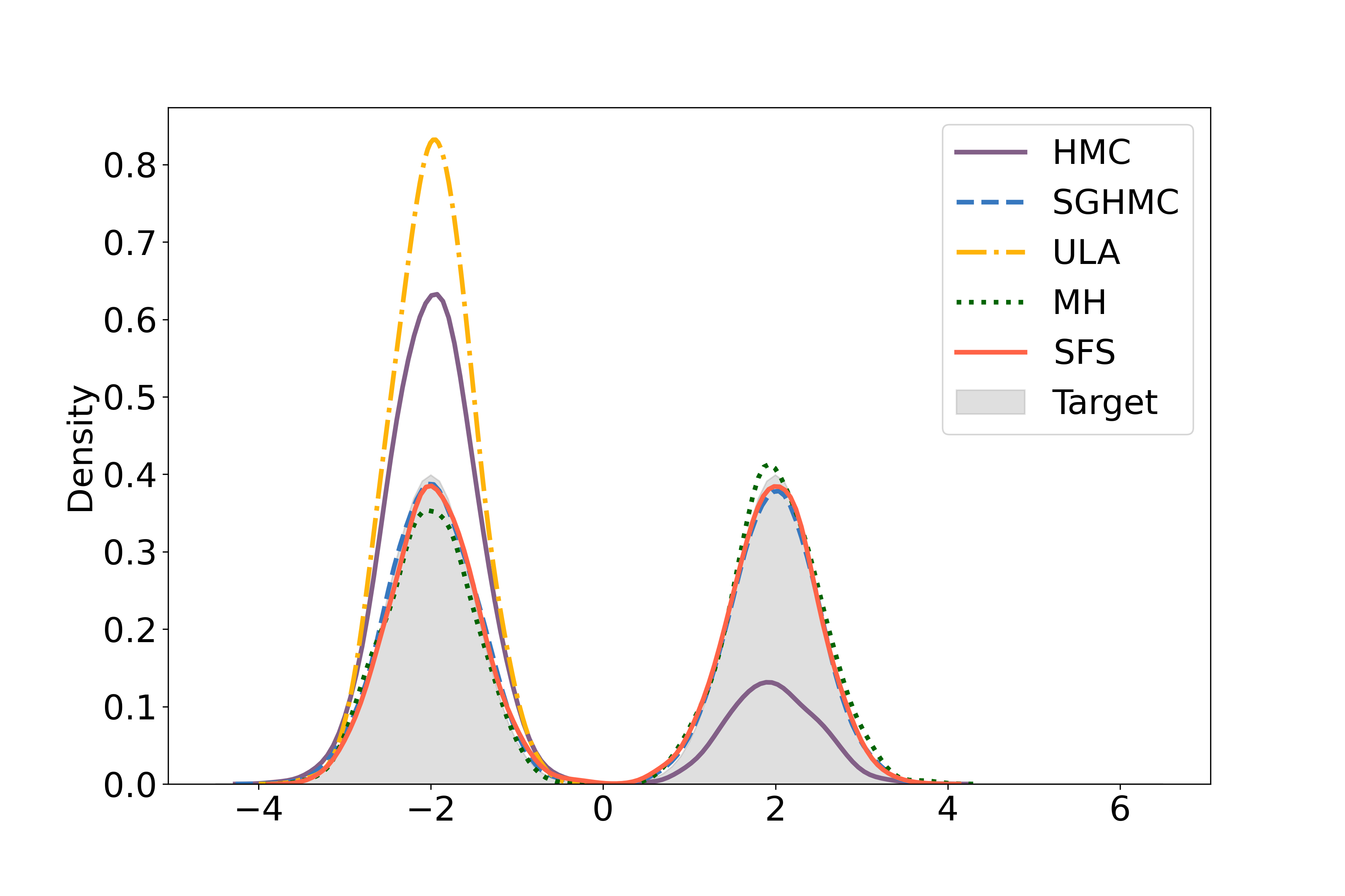
(a) $f_{1}(x)$

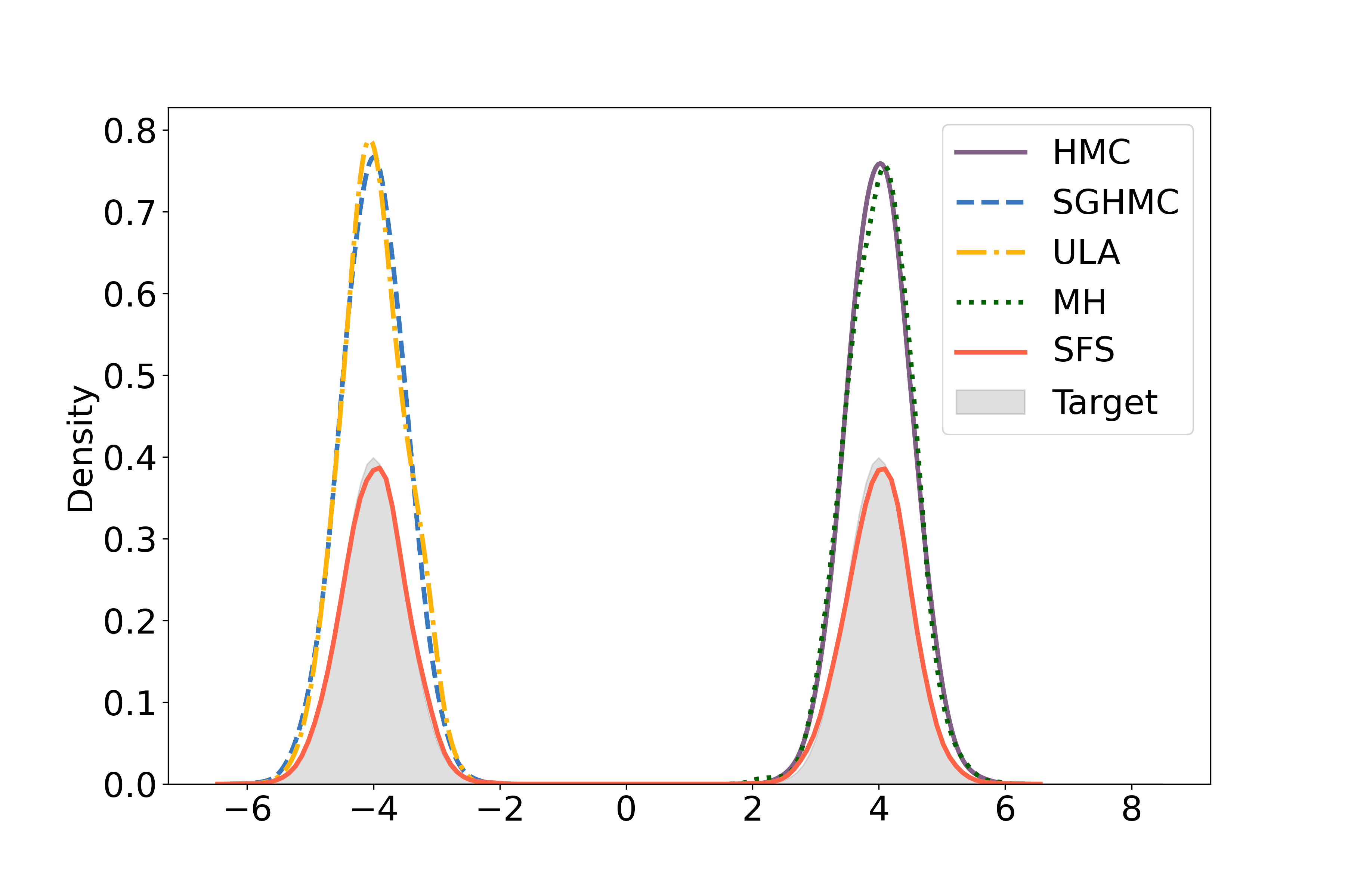
(b) $f_{2}(x)$

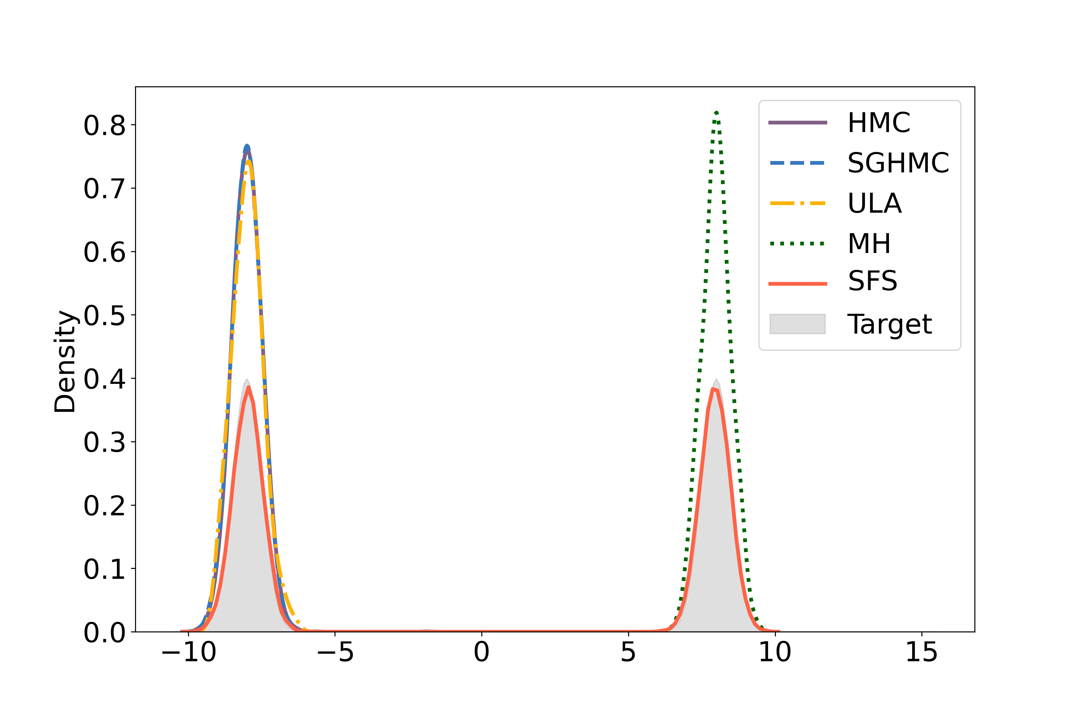
(c) $f_{3}(x)$

Figure 1: Kernel density estimation of one-dimensional Gaussian mixture distributions. The target distribution is shaded in grey.

6.2 Two-dimensional Gaussian mixture distribution

In this section, we consider four sets of two-dimensional Gaussian mixture distributions,

$$\kappa =4,8,16,~{}\alpha_{i}=\lambda_{1}(\sin(2(i-1)\pi/\kappa),\cos(2(i-1)\pi/\kappa)),~{}i=1,\cdots,\kappa,~{}\lambda_{1}=2,4,8,$$ (6.4)

$$\kappa =16,~{}\boldsymbol{\alpha}=(\lambda_{2}\{-3,-1,1,3\})^{\top}\times(\lambda_{2}\{-3,-1,1,3\}),~{}\lambda_{2}=1,1.5,2,$$ (6.5)

$$\kappa =25,~{}\boldsymbol{\alpha}=(\lambda_{3}\{-2,-1,0,1,2\})^{\top}\times(\lambda_{3}\{-2,-1,0,1,2\}),~{}\lambda_{3}=2,3,$$ (6.6)

$$\kappa =49,~{}\boldsymbol{\alpha}=(\lambda_{4}\{-3,-2,-1,0,1,2,3\})^{\top}\times(\lambda_{4}\{-3,-2,-1,0,1,2,3\}),~{}\lambda_{4}=2,3.$$ (6.7)

We set the proportions $\theta_{i}=1/\kappa$ and the covariance matrices $\Sigma_{i}=0.03\cdot\mathbf{I}_{2}$ across these settings. The centroids of Gaussian components gradually become farther apart across these scenarios for each setting. We set $N=20,000$, $K=100$ for model (6.4) and $K=200$ for the rest of the settings in Algorithm 1. The centroids of the Gaussian components in model (6.4) form a circle while those in (6.5)-(6.7) form a square matrix. For all models from (6.4) to (6.7), we employ the proposed SFS and other methods to generate samples and then visualize the kernel density estimation in Fig. 2-5, respectively.

As shown in Fig. 2-5 for models (6.4)-(6.7), only the samples from SFS succeed in estimating the underlying target distribution while all other methods collapse on one or a few modes when the models becomes more difficult to sample from. In model (6.4), although samples from MH, SGLD, SGHMC can give a density estimation that matches the underlying target in the simple case with four centroids in the first row of Fig. 2, they all fail to accurately sample from the target distribution when the numbers of components are bigger.

When the centroids from the mixture components form a square matrix shape, only the MH algorithm can perform as well as SFS in a simpler case (the first row of Fig. 3 to 5), all the other methods collapse on one or few modes. When the models become more difficult to sample from, mode collapsing for other methods becomes even worse. In all the simulations, we observe that only samples generated via SFS can accurately produce a density estimation that matches the underlying mixture distribution.

In general, we can draw the conclusion that SFS outperforms other algorithms, including MH, ULA, SGLD, SGHMC, cSGLD, NUTS and ACMC, through the visualization of two-dimensional Gaussian sampling.

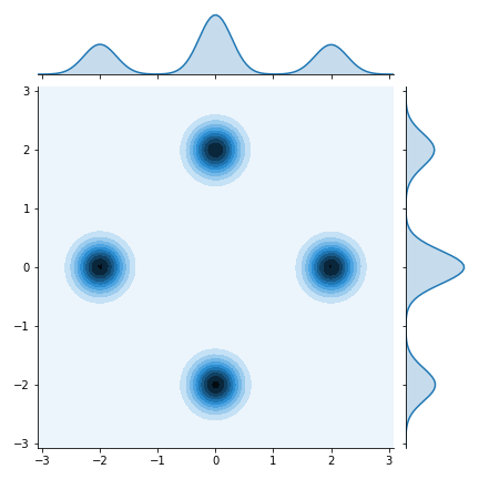
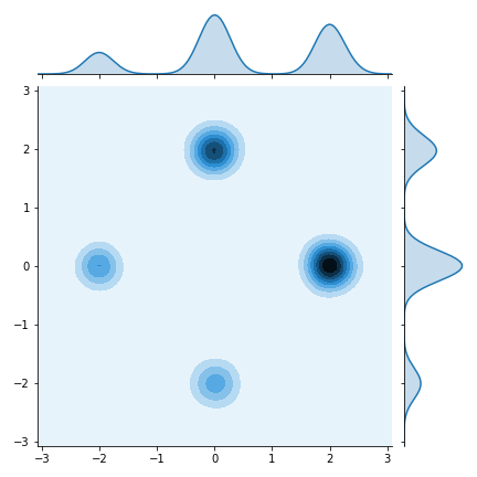
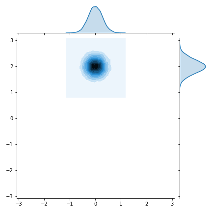
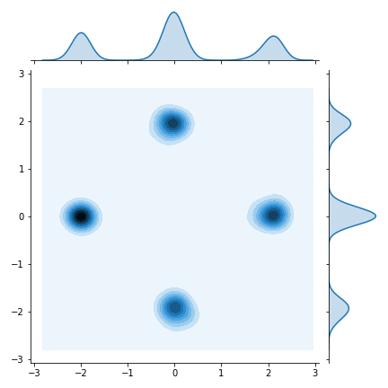
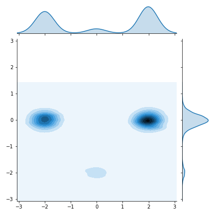
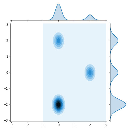
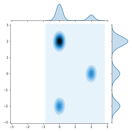
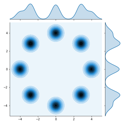
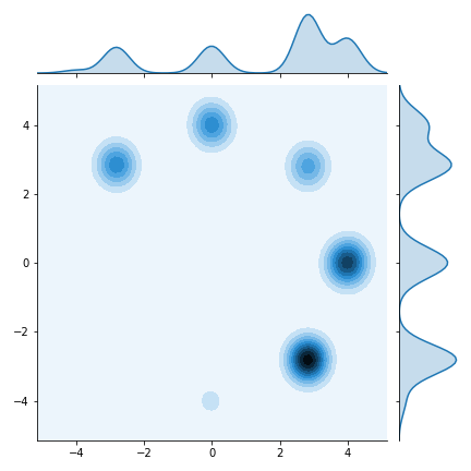
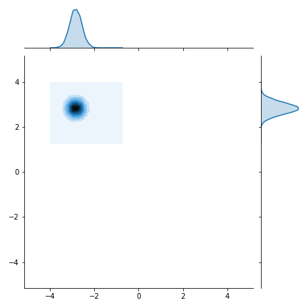
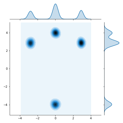
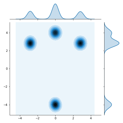
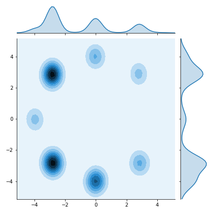
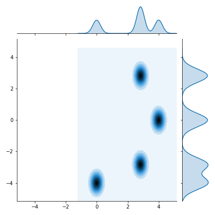
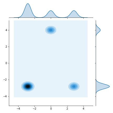
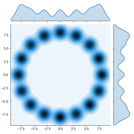
(a) SFS

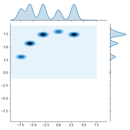
(b) MH

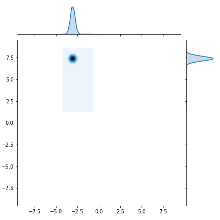
(c) ULA

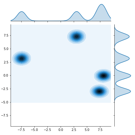
(d) SGLD

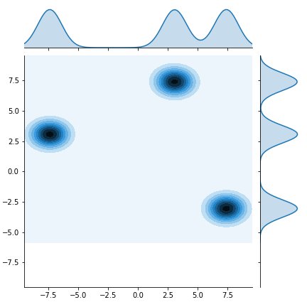
(e) SGHMC

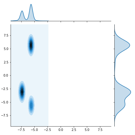
(f) cSGLD

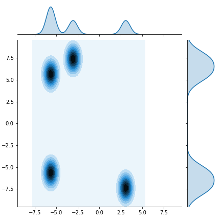
(g) NUTS

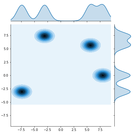
(h) ACMC

Figure 2: Kernel density estimation with marginal distribution plots for the circle shaped Gaussian mixture distributions. The number of Gaussian components $\kappa=4,8,16$ and the radius of the circle gradually increases from the top row to the bottom row.

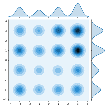
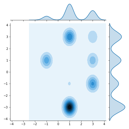
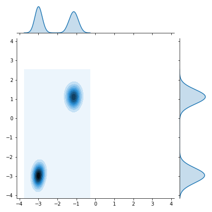
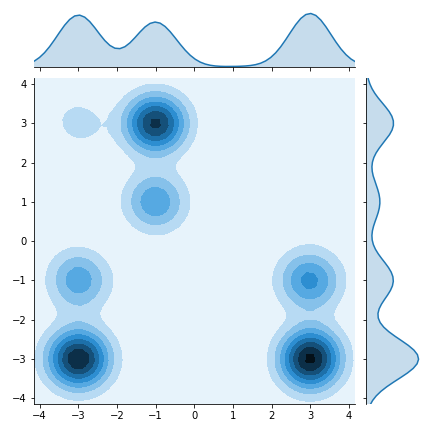
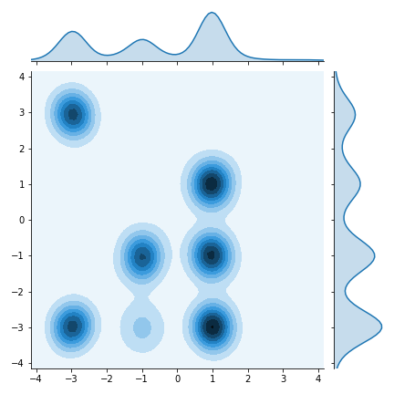
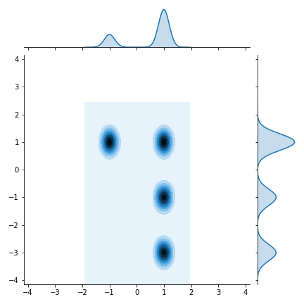
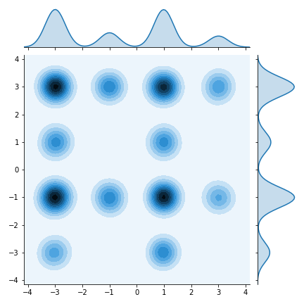
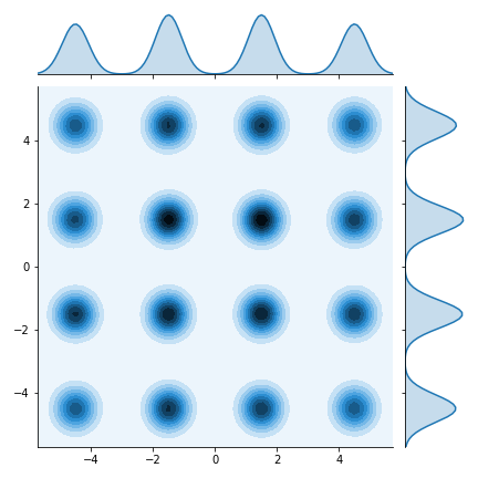
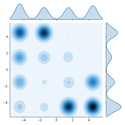
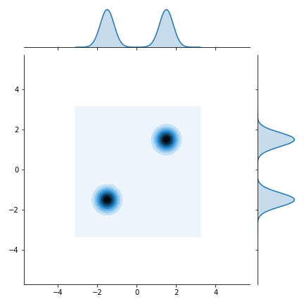
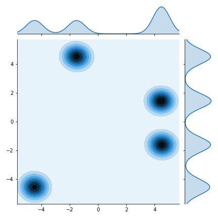
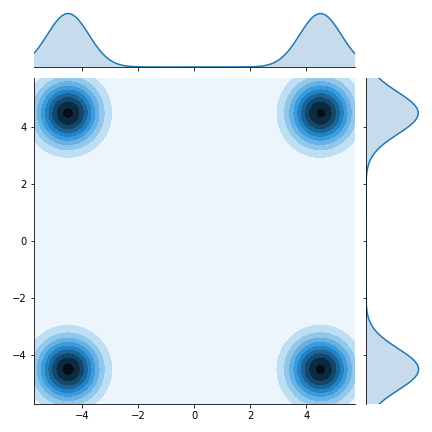
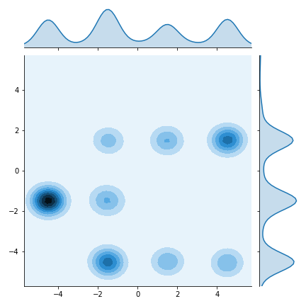
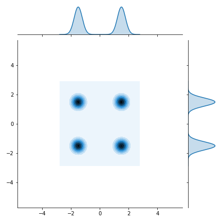
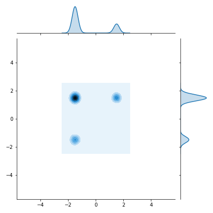
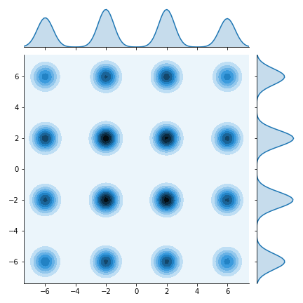
(a) SFS

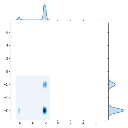
(b) MH

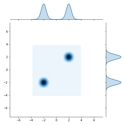
(c) ULA

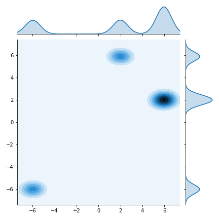
(d) SGLD

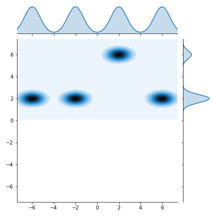
(e) SGHMC

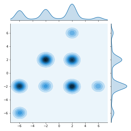
(f) cSGLD

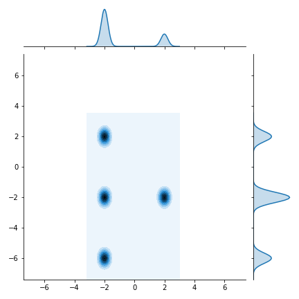
(g) NUTS

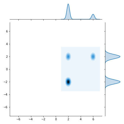
(h) ACMC

Figure 3: Kernel density estimation with marginal distribution plots for the 16-mode Gaussian mixture distributions. The distance between the neighboring modes gradually increases from the top row to the bottom row.

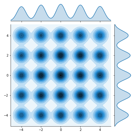
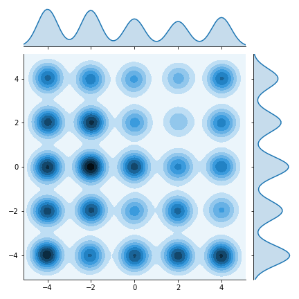
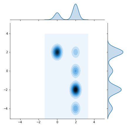
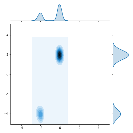
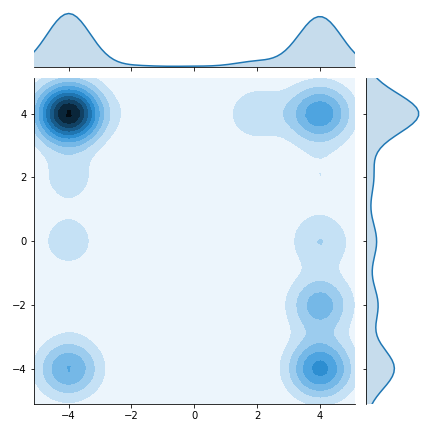
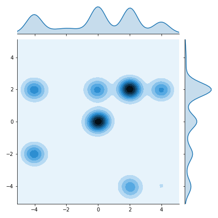
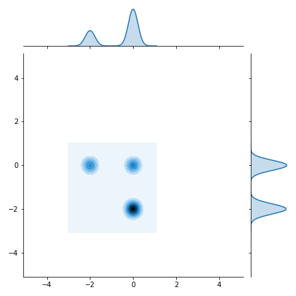
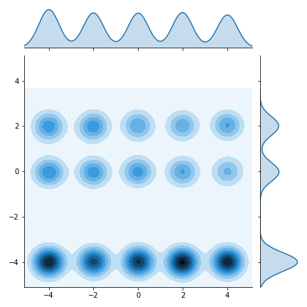
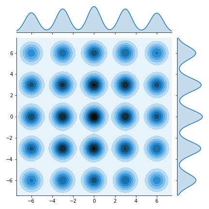
(a) SFS

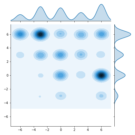
(b) MH

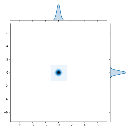
(c) ULA

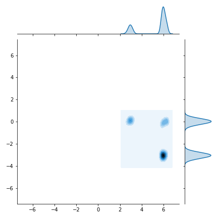
(d) SGLD

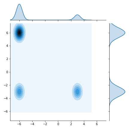
(e) SGHMC

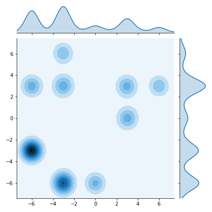
(f) cSGLD

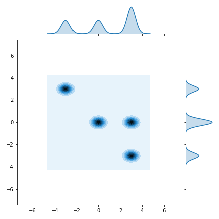
(g) NUTS

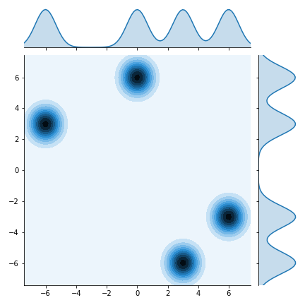
(h) ACMC

Figure 4: Kernel density estimation with marginal distribution plots for the 25-mode Gaussian mixture distributions. From the first row to the second row. The distance between the neighboring modes gradually increases.

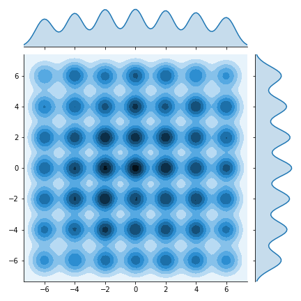
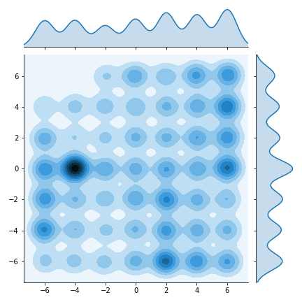
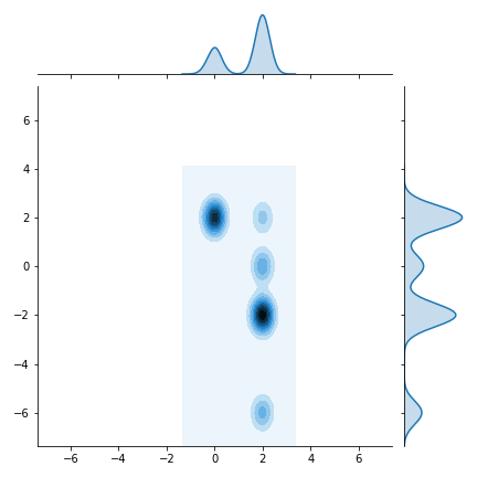
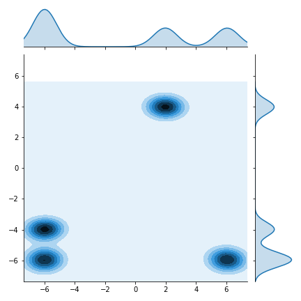
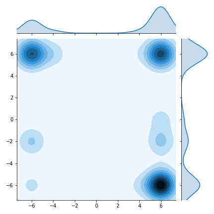
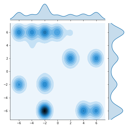
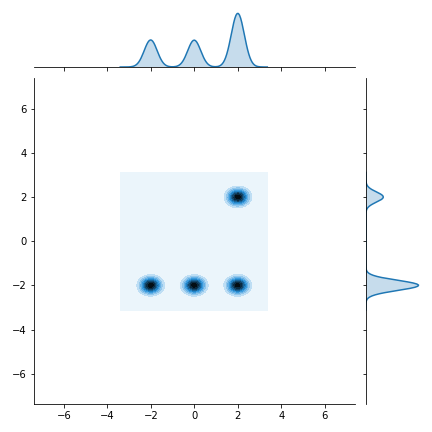
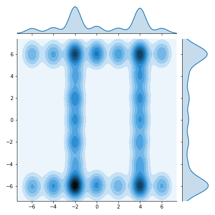
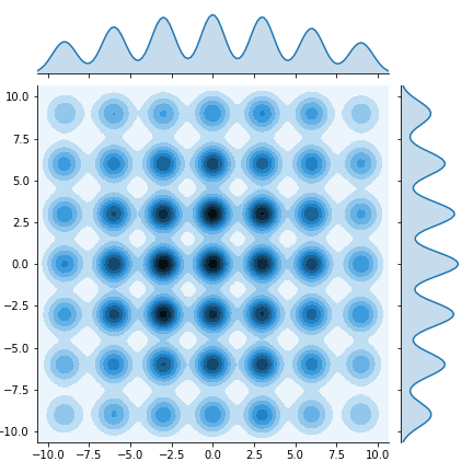
(a) SFS

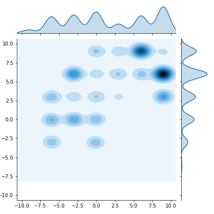
(b) MH

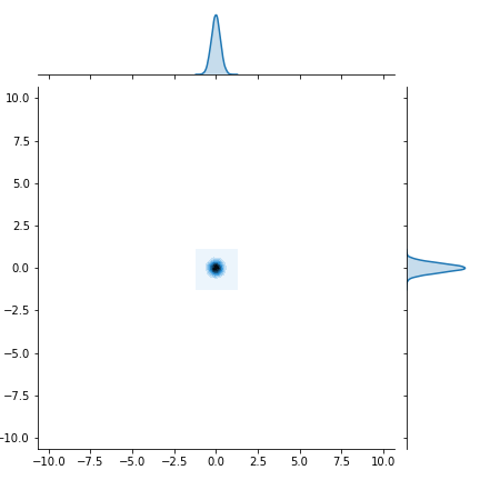
(c) ULA

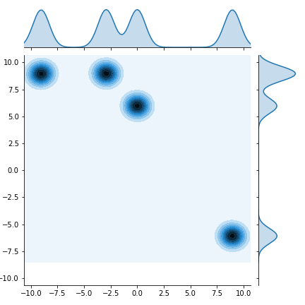
(d) SGLD

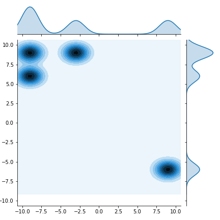
(e) SGHMC

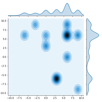
(f) cSGLD

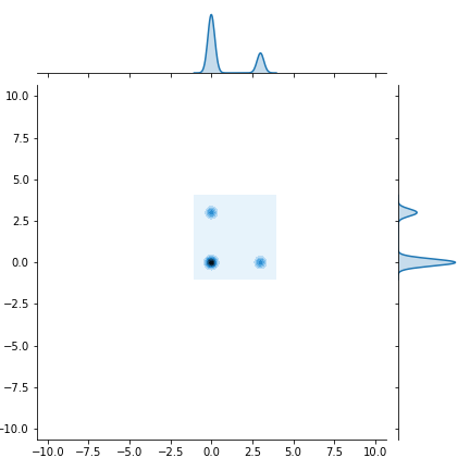
(g) NUTS

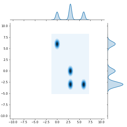
(h) ACMC

Figure 5: Kernel density estimation with marginal distribution plots for 49-mode Gaussian mixture distributions simulation. The distance between the neighboring modes gradually increases from the top row to the bottom row.

6.3 Evaluation of the balance of modes

We apply the $k$-means algorithm (MacQueen et al.,, 1967; Forgy,, 1965; Lloyd,, 1982) to estimate the proportions of the clusters using samples generated using SFS and the other methods consider here. In Fig. 6, we use dotted red lines for the true proportions in the target mixture distribution and color bars for the estimated proportions of the samples. Clearly, only the proportions of the components estimated based on the samples from SFS can accurately match the proportions of the components in the target mixture distribution of model (6.4), suggesting that SFS performs balanced sampling.

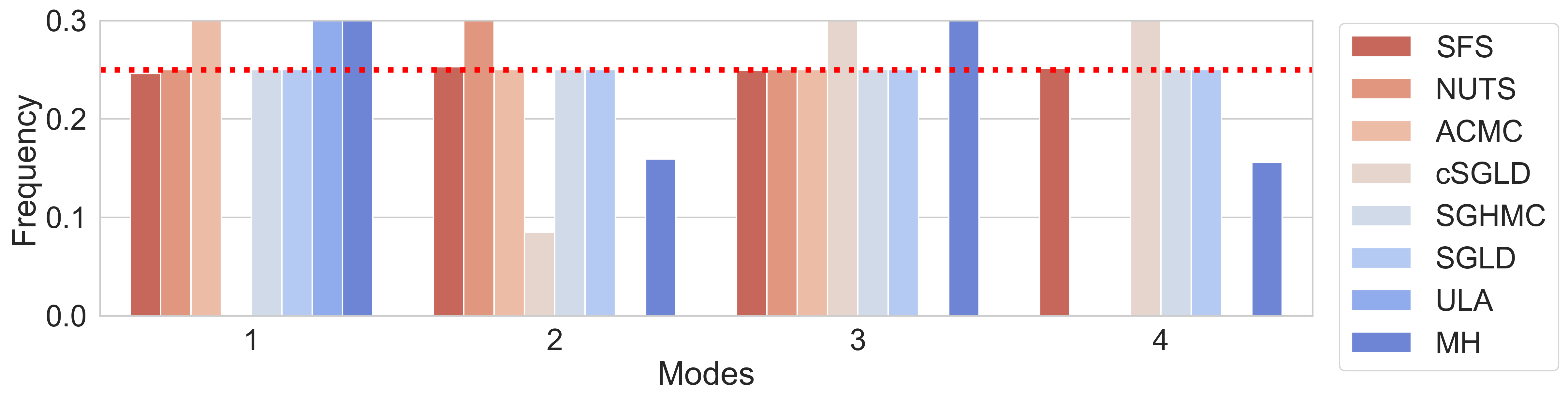
Scenario 1, $\lambda_{1}=2$

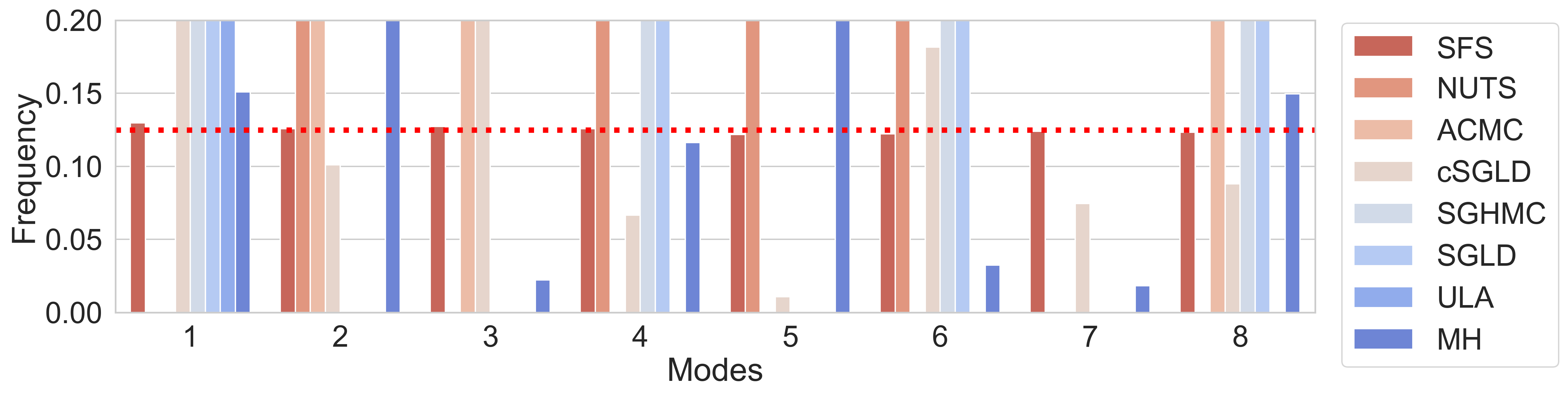
Scenario 2, $\lambda_{1}=4$

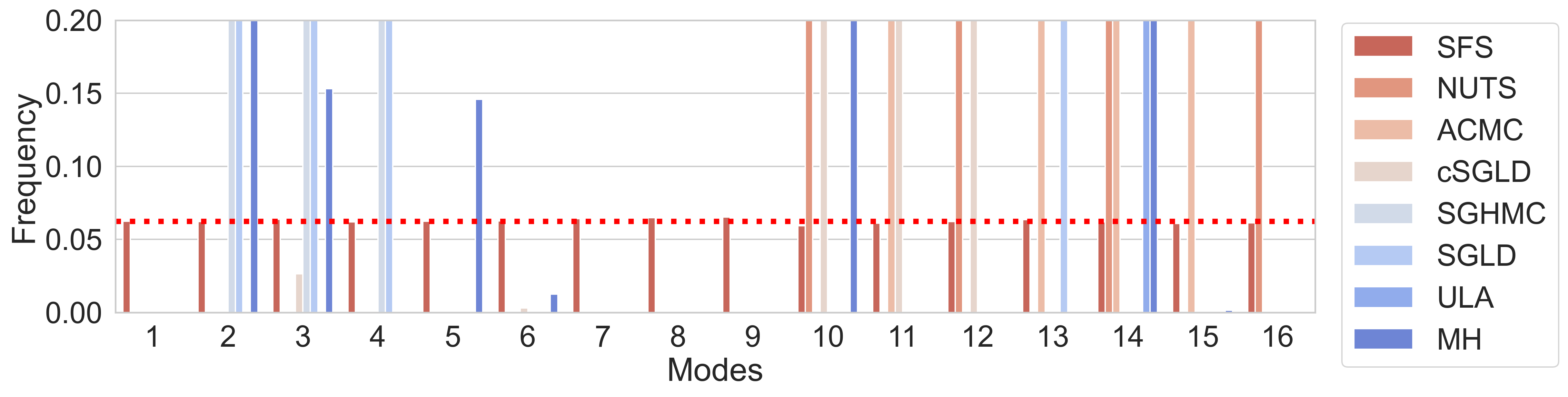
Scenario 3, $\lambda_{1}=8$

Figure 6: Frequency labeled by $k$-means on the circle shaped Gaussian mixture distributions simulation.

6.4 Bayesian logistic regression

Consider the binary logistic regression with an independent and identically distributed sample $\{x_{i},y_{i}\}_{i=1}^{n}$, that is,

$$P(y_{i}=1|x_{i})=\frac{\exp(x^{\top}_{i}\beta^{*})}{1+\exp(x^{\top}_{i}\beta^{*})},~{}i=1,\ldots,n,$$

where $x_{i}\in\mathbb{R}^{p}$ is the covariate vector, $y_{i}\in\{0,1\}$ is the response variable and $\beta^{*}=(\beta^{*}_{1},\ldots,\beta_{p}^{*})^{\top}\in\mathbb{R}^{p}$ is the vector of underlying regression coefficients. We draw samples for $\beta^{*}$ from its posterior distribution. Following (Durmus et al.,, 2019), (Durmus and Moulines,, 2016) and (Dalalyan, 2017b, ), we set the prior distribution of $\beta^{*}$ to be a Gaussian distribution with zero mean and covariance matrix $\Sigma_{\beta^{*}}=(\sum_{i=1}^{n}x_{i}x_{i}^{\top}/n)^{-1}$, then the posterior distribution of $\beta^{*}$ is expressed as

$$\mu(\beta^{*})\propto\exp\left(\sum_{i=1}^{n}\left(y_{i}x_{i}^{\top}\beta^{*}-\log(1+\exp(x_{i}^{\top}\beta^{*}))\right)-{\beta^{*}}^{\top}\Sigma_{\beta^{*}}^{-1}\beta^{*}/2\right).$$ (6.8)

Also, as in (Durmus et al.,, 2019), (Durmus and Moulines,, 2016) and (Dalalyan, 2017b, ), we set $n=1000$ and $p=5$. The covarites vector $\{x_{i}\}_{i=1}^{n}$ are independent and identically distributed from $N(0,\Sigma)$, where $\Sigma_{i,j}=0.5^{|i-j|}$ for $1\leq i,j\leq p$. In Algorithm 2, we set $K=200$ and $m=1000$. We generate a random sample with sample size $N=10,000$ using the proposed SFS, MH algorithm and ULA. We compare SFS with MH algorithm and ULA in term of the sample mean (Mean), sample median (Med) and sample variance (Var). The results are reported in Table 1 and Fig. 7 and 8 below.

In Table 1, the first column describes the methods; the second column shows the criterions including Mean, Med and Var; the values in brackets are the true value of underlying regression coefficients $\beta^{*}_{i}$ with $i=1,\ldots,5$. For the proposed method, the values of Mean and Med are close to the true values of $\beta^{*}$ except $\beta_{2}^{*}$, while it still takes more accurate values than MH algorithm and ULA in $\beta_{2}^{*}$, and the values of Var are slightly larger than other two methods. Especially, MH algorithm takes the values trifle away from $\beta^{*}_{1}$, $\beta^{*}_{2}$, $\beta^{*}_{4}$ and $\beta^{*}_{5}$ in Mean and Med.

Fig. 7 shows the box plots of samples for SFS, MH algorithm and ULA, where the horizontal dotted red lines are the ground truth of the coefficients. We can see that the samples of SFS match the ground truth better than MH algorithm and ULA.

Fig. 8 depicts the curves of kernel density estimation and true values for each component of $\beta^{*}$. In this figure, the red solid lines and the corresponding red shades are the kernel density estimation of SFS, while the blue and green lines correspond to the MH algorithm and ULA respectively, and the red dotted lines perpendicular to the horizontal axis represent the value of $\beta_{i}^{*}$ with $i=1,\dots,5$. Except for $\beta^{*}_{2}$, the rest $\beta^{*}_{i}$ coincide with the peaks of kernel density estimation curves of the proposed method. But, $\beta_{2}^{*}$ and $\beta_{3}^{*}$ keep away from the peaks of the kernel density estimation curves of ULA, and each component of $\beta^{*}$ is not close to that of MH algorithm.

Table 1: Numerical results of the binary Bayesian logistic regression.

Method	Criterions	$\beta^{*}_{1}$ (0.220)	$\beta^{*}_{2}$ (0.208)	$\beta^{*}_{3}$ (-2.027)	$\beta^{*}_{4}$ (0.744)	$\beta^{*}_{5}$ (1.424)
SFS	Mean	0.206	0.307	-2.033	0.716	1.372
	Med	0.205	0.316	-2.068	0.724	1.390
	Var	0.041	0.049	0.098	0.049	0.057
MH	Mean	0.279	0.415	-2.286	0.862	1.560
	Med	0.336	0.469	-2.321	0.965	1.556
	Var	0.010	0.018	0.015	0.029	0.003
ULA	Mean	0.219	0.372	-2.214	0.780	1.461
	Med	0.220	0.371	-2.213	0.776	1.463
	Var	0.011	0.013	0.027	0.016	0.014

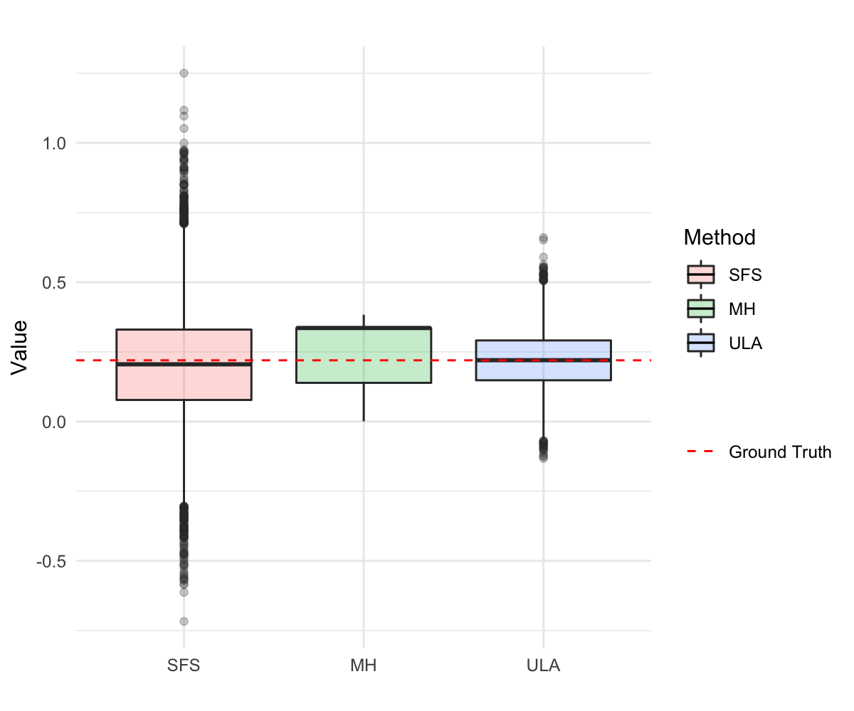
(a) $\beta_{1}^{*}$

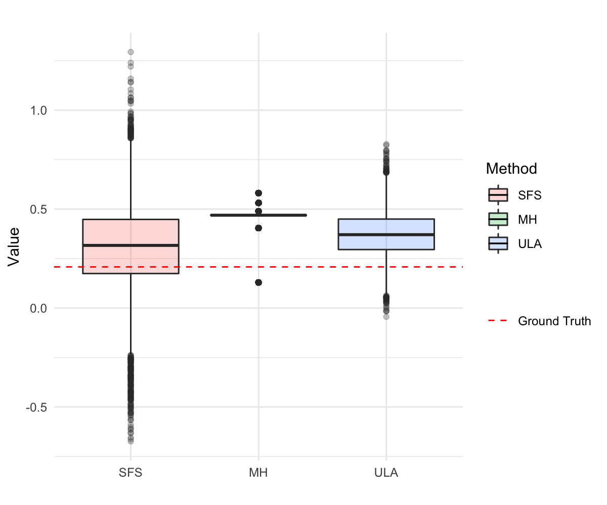
(b) $\beta_{2}^{*}$

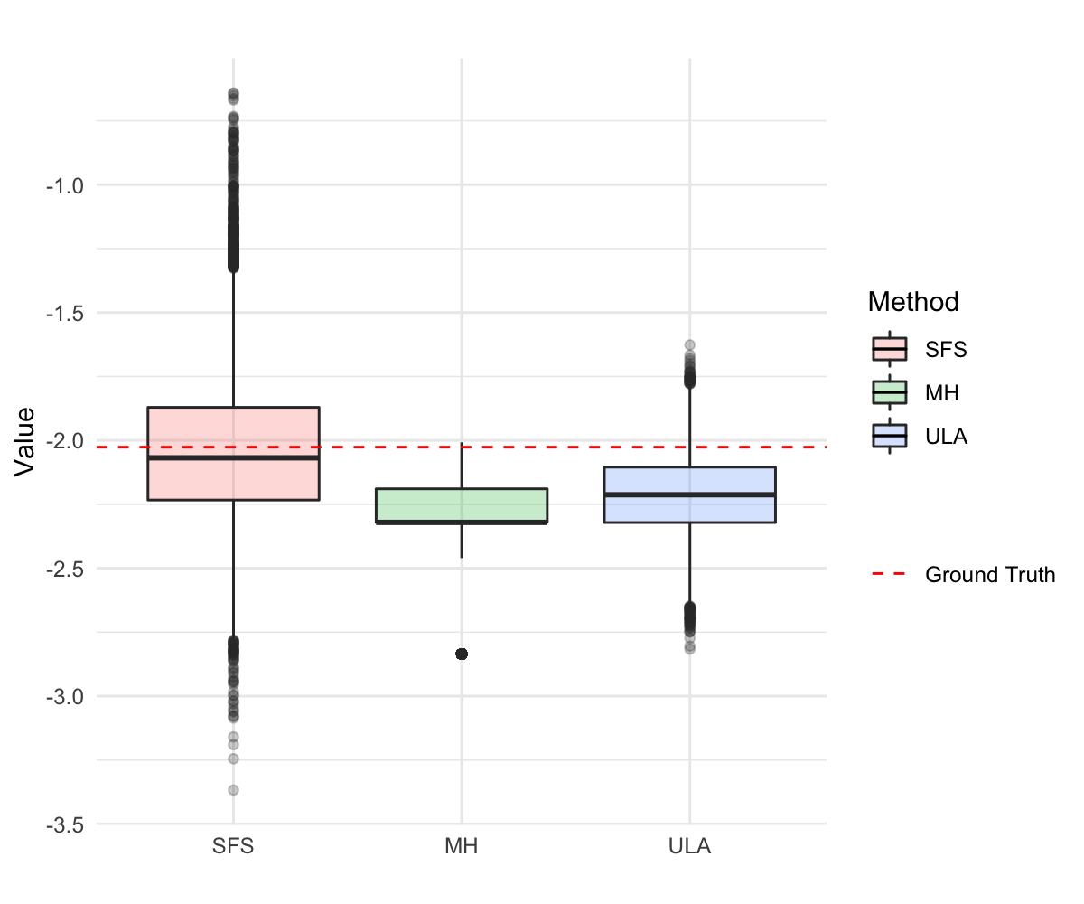
(c) $\beta_{3}^{*}$

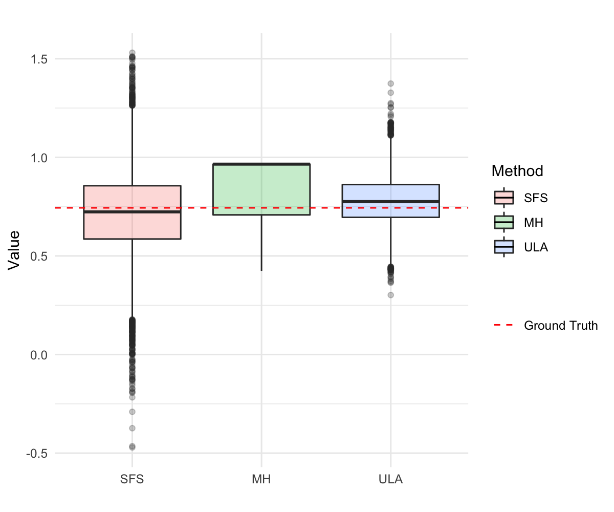
(d) $\beta_{4}^{*}$

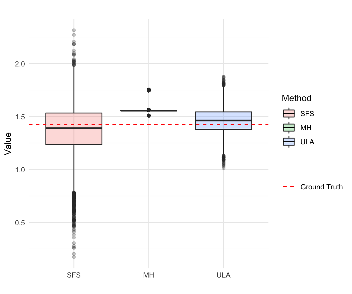
(e) $\beta_{5}^{*}$

Figure 7: Box plots of the binary Bayesian logistic regression with $N=10,000$ for $\beta_{1}^{*},\dots,\beta_{5}^{*}$. The horizontal dotted red lines are the ground truth of the coefficients.

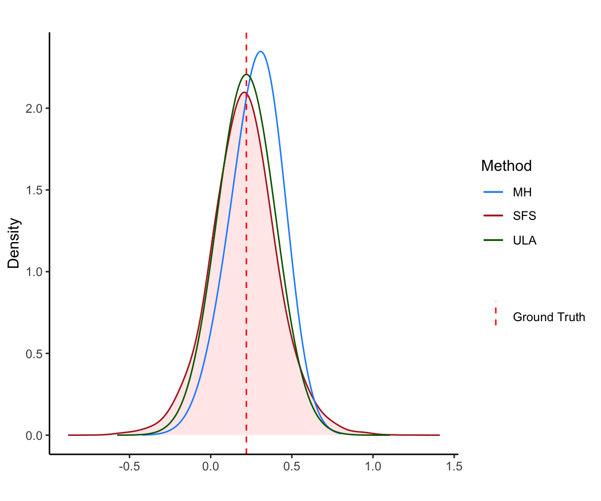
(a) $\beta_{1}^{*}$

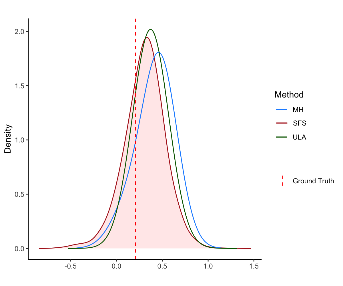
(b) $\beta_{2}^{*}$

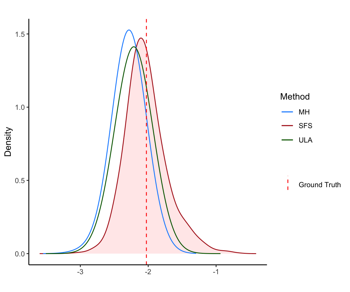
(c) $\beta_{3}^{*}$

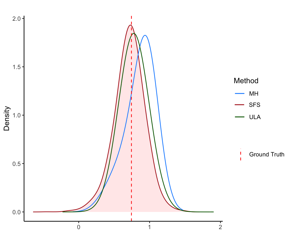
(d) $\beta_{4}^{*}$

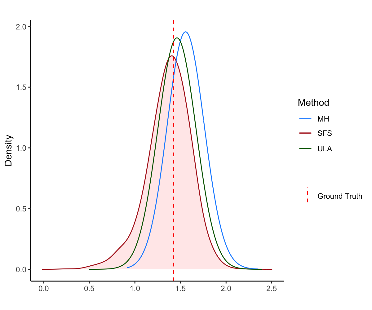
(e) $\beta_{5}^{*}$

Figure 8: Kernel density estimation of the binary Bayesian logistic regression with $N=10,000$ for $\beta_{1}^{*},\dots,\beta_{5}^{*}$. The red solid lines and the corresponding red shades are the estimated density curves of the proposed method, and the blue and green lines correspond to the MH algorithm and ULA respectively. The vertical dotted red lines are the ground truth of the coefficients.

To demonstrate the unbiasedness and coverage rates, we use the same experimental setting for the binary Bayesian logistic regression, except that $p=3$. We generate 100 replicates of random samples with sample size $N=1,000$ using the proposed SFS, MH algorithm and ULA.

The absolute errors and ordinary errors are respectively reported with the box plots in the Figure 9 and 10. As Figure 9 shows, the performance of SFS and other algorithms is comparable in terms of estimation accuracy. We can conclude from the box plots of errors in Figure 10 that the estimation of SFS is unbiased based on the experimental simulation. We demonstrate the coverage rate of the 95% confidence interval for the true coefficient in Table 2, which is based on the random samples we generate from the posterior distribution. We can see that the coverage rate of the confidence interval based on SFS approaches 95%, which is generally comparable to that of ULA and MH algorithm.

We apply SFS to the real data classification tasks to compare ULA and MH algorithm. The dataset Diabetes (Smith et al.,, 1988) aims to predict whether a person has diabetes according to health measurements. The objective of the dataset German (Dua and Graff,, 2017) is to classify good or bad credit risks. We need to classify the survival status in the dataset Haberman (Haberman,, 1976; Dua and Graff,, 2017) based on the descriptions of patients. The aim of the dataset Vc (Berthonnaud et al.,, 2005; Dua and Graff,, 2017) is to predict orthopaedic patients into normal or abnormal. The sample size, attribute number and URL of these data are shown in Table 3. We can conclude from the prediction accuracy shown in Figure 11 that SFS outperforms the other two methods.

7 Conclusion

We propose SFS method for sampling from distributions via the Euler-Maruyama discretization of Schrödinger-Föllmer diffusion defined on the unite time interval $[0,1]$. A prominent feature of SFS is that it does not require the underlying Markov process to be ergodic to generate samples from the target distribution while ergodicity is needed for other MCMC samplers. We establish non-asymptotic error bounds for the sampling distribution of the SFS in the Wasserstein distance under appropriate conditions. In particular, when the drift term can be evaluated analytically, we only need some smoothness conditions on the target distribution to ensure the error bounds for samples generated in Algorithm 1. For the drift term without analytical expression, we further propose to generate samples in Algorithm 2 using the Monte Carlo estimation and establish the consistency of Algorithm 2. Our numerical experiments demonstrate that SFS can enlarge the scope of existing samplers for sampling in multi-mode distributions possibly without normalization. Therefore, the proposed SFS can be a useful addition to the existing methods for sampling from possibly unnormalized distributions.

Several problems deserve further study. For example, for the samples generated from Algorithm 2, we show its convergence under a strong convexity condition on the potential. It would be interesting to weaken or even remove this condition. This is an interesting and challenging technical problem. Applying SFS to more Bayesian inference with more complex real data is also of immense interest.

Table 2: Coverage rates of the binary Bayesian logistic regression (100 replicates).

Components	1	2	3
SFS	99 %	98 %	99 %
MH	93 %	95 %	96 %
ULA	98 %	98 %	100 %

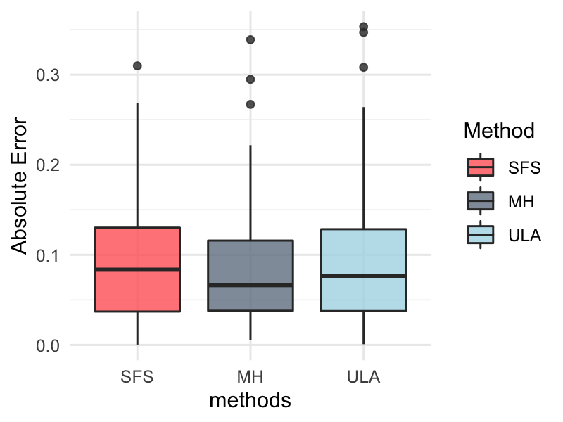
(a) $\beta_{1}^{*}$

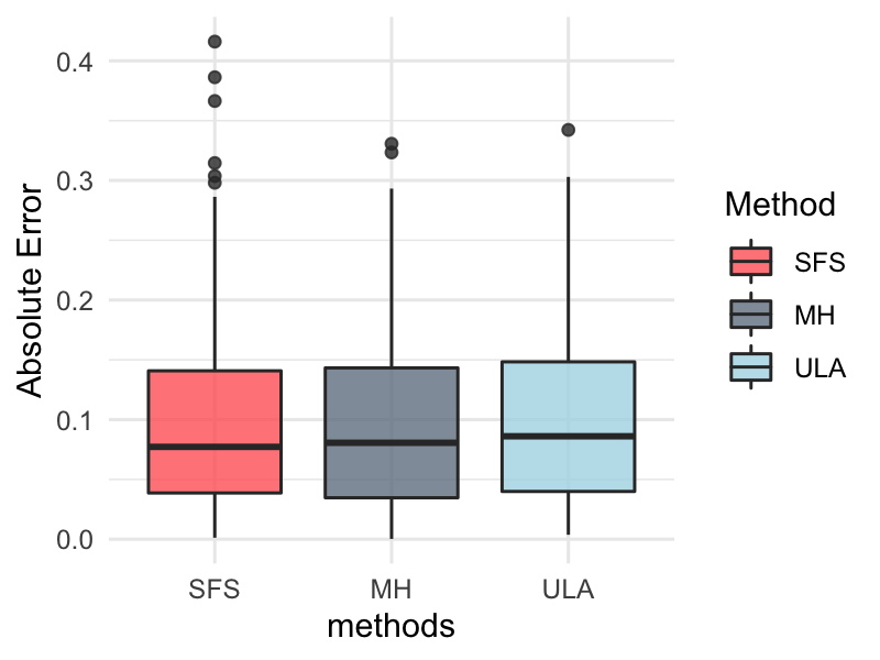
(b) $\beta_{2}^{*}$

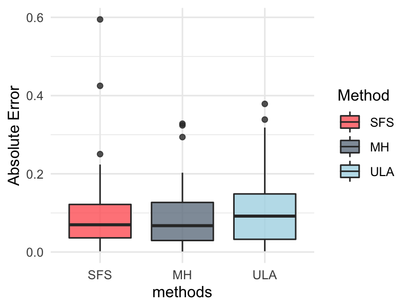
(c) $\beta_{3}^{*}$

Figure 9: Box plots of absolute errors on the binary Bayesian logistic regression with $N=1,000$ for $\beta_{1}^{*},\dots,\beta_{3}^{*}$.

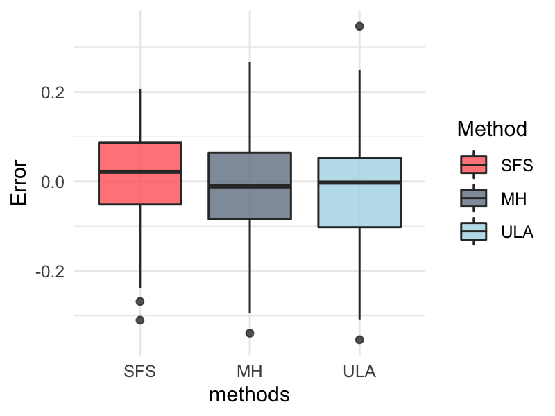
(a) $\beta_{1}^{*}$

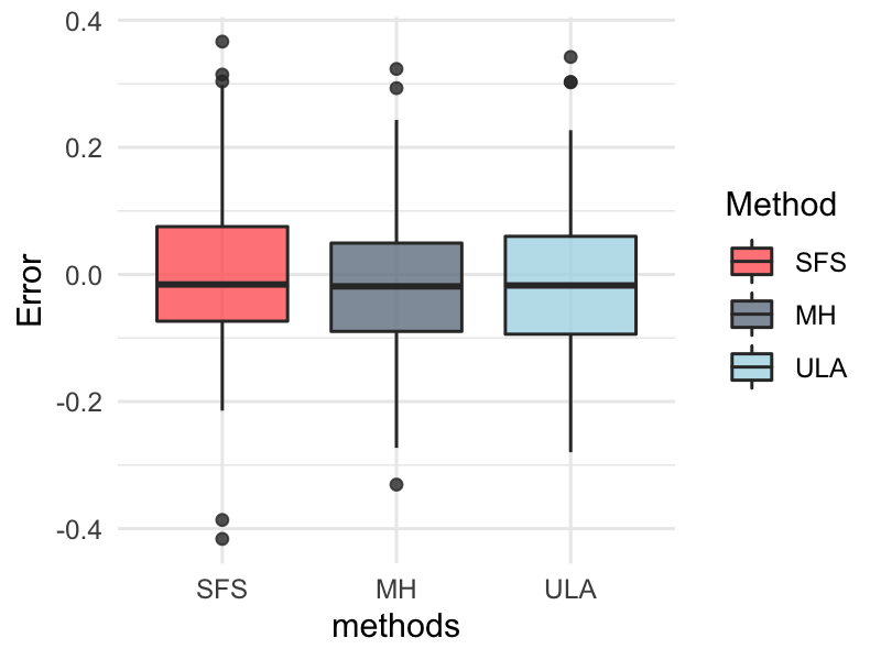
(b) $\beta_{2}^{*}$

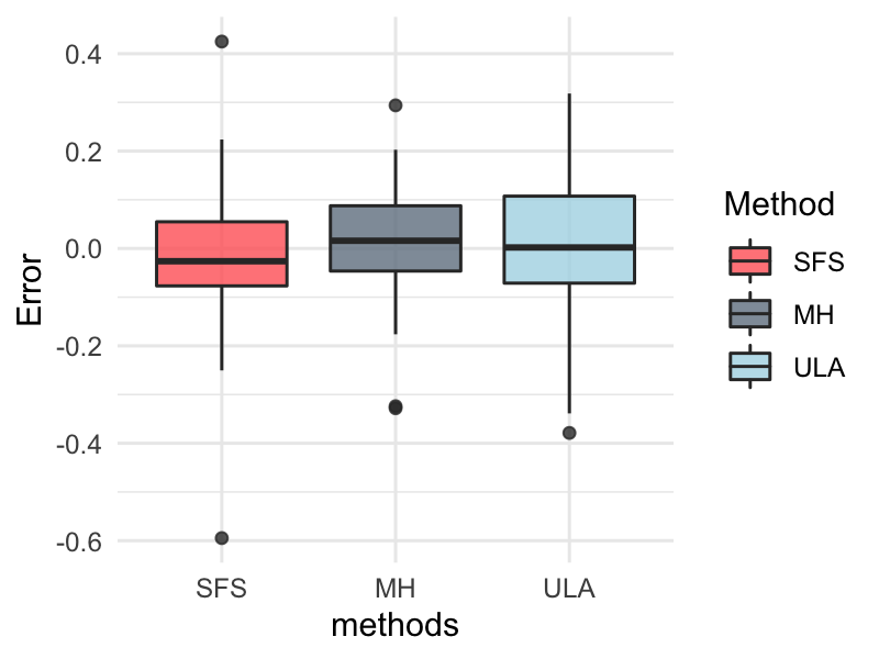
(c) $\beta_{3}^{*}$

Figure 10: Box plots of errors on the binary Bayesian logistic regression with $N=1,000$ for $\beta_{1}^{*},\dots,\beta_{3}^{*}$.

Table 3: Descriptions on real datasets.

Dataset	# Sample	# Attributes	URL
Diabetes	768	8	https://www.kaggle.com/uciml/pima-indians-diabetes-database
German	1000	20	https://archive.ics.uci.edu/ml/datasets/statlog+(german+credit+data)
Haberman	306	3	https://archive.ics.uci.edu/ml/datasets/haberman’s+survival
Vc	310	6	https://archive.ics.uci.edu/ml/datasets/Vertebral+Column

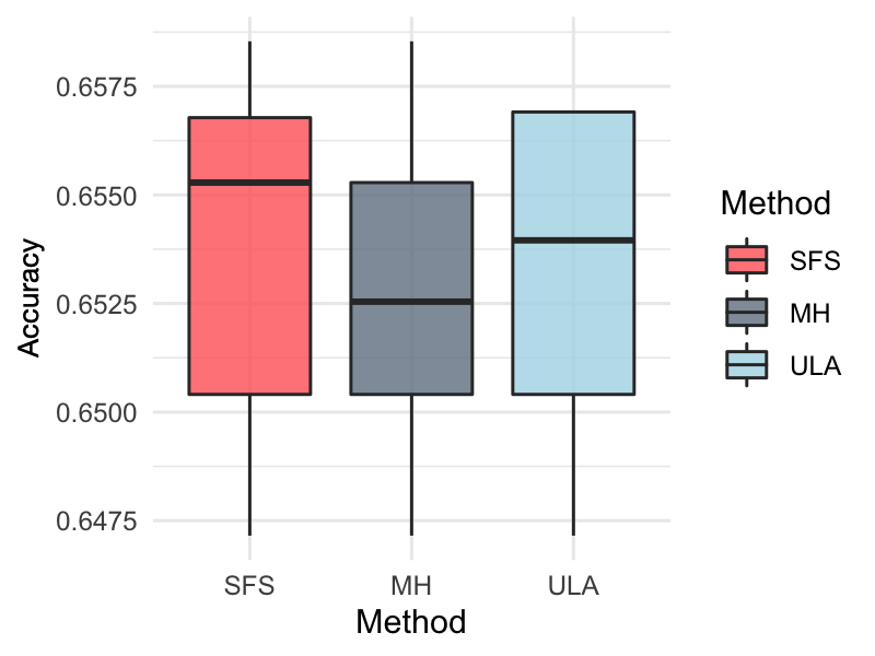
(a) Diabetes

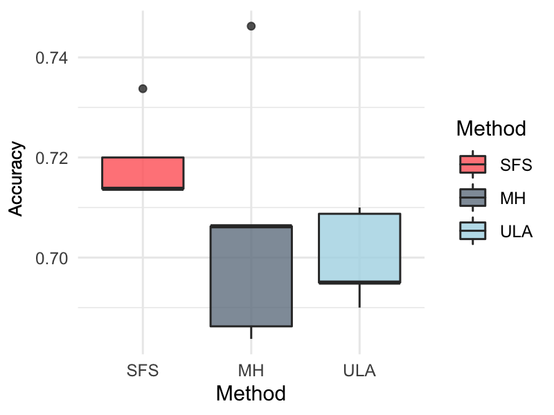
(b) German

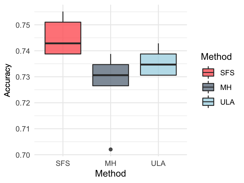
(c) Haberman

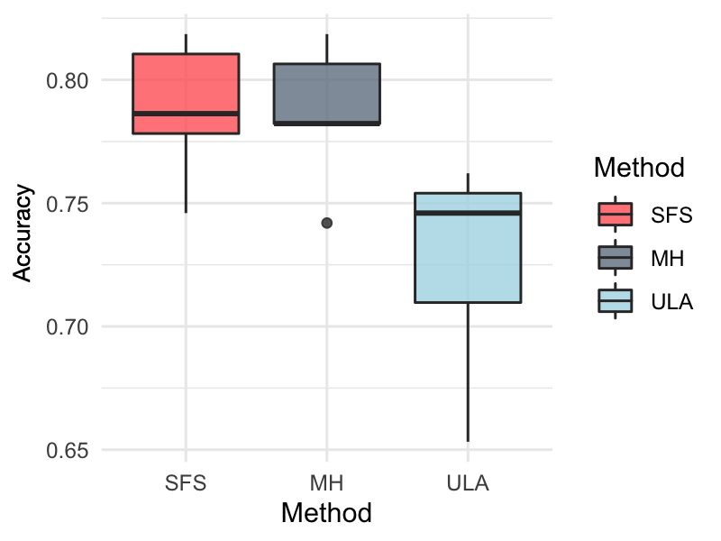
(d) Vc

Figure 11: Prediction accuracies on real data with SFS, ULA and MH algorithm; for each dataset, we evaluate these methods by selecting training and validation sets randomly for five times.

8 Acknowledgments

The authors would like to thank Dr. Francisco Vargas at Department of Computer Science, Cambridge University for helpful discussion.

J. Huang is partially supported by the U.S. NSF grant DMS-1916199. Y. Jiao is supported in part by the National Science Foundation of China under Grant 11871474 and by the research fund of KLATASDSMOE of China. J. Liu is supported by the grants MOE2018-T2-1-046 and MOE2018-T2-2-006 from the Ministry of Eduction, Singapore. The numerical studies of this work were done on the supercomputing system in the Supercomputing Center of Wuhan University.

Appendix A Appendix

In the appendix, we prove Proposition 2.1, Remark 4.1 and Theorems 4.1-4.4. We note that Proposition 2.1 is a known result (see, e.g., Föllmer, (1985, 1986); Tzen and Raginsky, (2019)). We include a proof here for ease of reference.

A.1 Proof of Proposition 2.1

Proof.

It is well-known that the transition probability density of a standard $p$-dimensional Brownian motion is given by

$$\widetilde{p}_{s,t}(x,y)=\frac{1}{(2\pi(t-s))^{p/2}}\exp\left(-\frac{1}{2(t-s)}\|x-y\|^{2}_{2}\right).$$

This implies that the diffusion process $\{X_{t}\}_{t\in[0,1]}$ defined in (2.1) admits the transition probability density

$$p_{s,t}(x,y)=\widetilde{p}_{s,t}(x,y)\frac{Q_{1-t}f(y)}{Q_{1-s}f(x)}.$$

It follows that for any measurable set $A\in\mathcal{B}(\mathbb{R}^{p})$,

$$P(X_{1}\in A) =\int_{A}p_{0,1}(0,y)\mathrm{d}y$$

$$=\int_{A}\widetilde{p}_{0,1}(0,y)\frac{Q_{0}f(y)}{Q_{1}f(0)}\mathrm{d}y$$

$$=\mu(A).$$

Therefore, $X_{1}$ is distributed as the probability distribution $\mu$. This completes the proof. ∎

A.2 Drift term $b(x,t)$ for Gaussian mixture distribution (2.12)

We derive the expression of the drift term $b(x,t)$ in (2.12) for the Gaussian mixture distribution.

Proof.

For $Z\sim N(0,\mathbf{I}_{p})$, we have

$$\mathbb{E}_{Z}f_{i}(x+\sqrt{1-t}Z)$$

$$=\mathbb{E}_{Y\sim N(x,(1-t)\mathbf{I}_{p})}f_{i}(Y)$$

$$=\frac{1}{|\Sigma_{i}|^{1/2}}\cdot\mathbb{E}_{Y\sim N(x,(1-t)\mathbf{I}_{p})}\exp\left(\frac{\|Y\|_{2}^{2}-(Y-\alpha_{i})^{\top}\Sigma_{i}^{-1}(Y-\alpha_{i})}{2}\right)$$

$$=\frac{1}{(2\pi(1-t))^{p/2}|\Sigma_{i}|^{1/2}}\int\exp\left(\frac{\|y\|^{2}}{2}-\frac{(y-\alpha_{i})^{\top}\Sigma_{i}^{-1}(y-\alpha_{i})}{2}-\frac{\|y-x\|^{2}_{2}}{2-2t}\right)dy$$

$$=\frac{g_{i}(x,t)}{|t\Sigma_{i}+(1-t)\mathbf{I}_{p}|^{1/2}}.$$ (A.1)

where

$$g_{i}(x,t) =\exp\left(\frac{1}{2-2t}\|(t\mathbf{I}_{p}+(1-t)\Sigma_{i}^{-1})^{-1/2}((1-t)\Sigma_{i}^{-1}\alpha_{i}+x)\|_{2}^{2}\right)$$

$$~{}~{}~{}~{}\times\exp\left(-\frac{1}{2}\alpha_{i}^{T}\Sigma_{i}^{-1}\alpha_{i}-\frac{1}{2-2t}\|x\|_{2}^{2}\right).$$

Similarly, we have

$$\mathbb{E}_{Z}\nabla f_{i}(x+\sqrt{1-t}Z)$$

$$=\mathbb{E}_{Y\sim N(x,(1-t)\mathbf{I}_{p})}\nabla f_{i}(Y)$$

$$=\frac{\Sigma_{i}^{-1}\alpha_{i}}{|\Sigma_{i}|^{1/2}}\cdot\mathbb{E}_{Y\sim N(x,(1-t)\mathbf{I}_{p})}\exp\left(\frac{\|Y\|_{2}^{2}-(Y-\alpha_{i})^{\top}\Sigma_{i}^{-1}(Y-\alpha_{i})}{2}\right)$$

$$~{}~{}~{}+\frac{\mathbf{I}_{p}-\Sigma_{i}^{-1}}{|\Sigma_{i}|^{1/2}}\cdot\mathbb{E}_{Y\sim N(x,(1-t)\mathbf{I}_{p})}Y\cdot\exp\left(\frac{\|Y\|_{2}^{2}-(Y-\alpha_{i})^{\top}\Sigma_{i}^{-1}(Y-\alpha_{i})}{2}\right)$$

$$=\frac{\Sigma_{i}^{-1}\alpha_{i}}{|\Sigma_{i}|^{1/2}}\cdot\int\frac{1}{(2\pi(1-t))^{p/2}}\exp\left(\frac{\|y\|^{2}}{2}-\frac{(y-\alpha_{i})^{\top}\Sigma_{i}^{-1}(y-\alpha_{i})}{2}-\frac{\|y-x\|^{2}_{2}}{2-2t}\right)dy$$

$$~{}~{}~{}+\frac{\mathbf{I}_{p}-\Sigma_{i}^{-1}}{|\Sigma_{i}|^{1/2}}\cdot\int\frac{y}{(2\pi(1-t))^{p/2}}\exp\left(\frac{\|y\|^{2}}{2}-\frac{(y-\alpha_{i})^{\top}\Sigma_{i}^{-1}(y-\alpha_{i})}{2}-\frac{\|y-x\|^{2}_{2}}{2-2t}\right)dy$$

$$=\frac{\Sigma_{i}^{-1}\alpha_{i}+(\mathbf{I}_{p}-\Sigma_{i}^{-1})[t\mathbf{I}_{p}+(1-t)\Sigma_{i}^{-1}]^{-1}[(1-t)\Sigma_{i}^{-1}\alpha_{i}+x]}{|t\Sigma_{i}+(1-t)\mathbf{I}_{p}|^{1/2}}\cdot g_{i}(x,t).$$ (A.2)

Hence, the analytical expression of $b(x,t)$ in (2.13) is obtained by plugging the expressions (A.2) and (A.2) into (2.13). ∎

A.3 Proof of Remark 4.1

Proof.

Since $g$ and $\nabla g$ are Lipschitz continuous, there exists a finite and positive constant $\gamma$ such that for all $x,y\in\mathbb{R}^{p}$,

$$|g(x)-g(y)|\leq\gamma\|x-y\|_{2},$$ (A.3)

$$\|\nabla g(x)-\nabla g(y)\|_{2}\leq\gamma\|x-y\|_{2}.$$ (A.4)

Moreover, since $g$ has a lower bound greater than 0, there exists a finite and positive constant $\xi$ such that

$$g\geq\xi>0.$$ (A.5)

By (A.3) and (A.5), it yields that for all $x\in\mathbb{R}^{p}$ and $t\in[0,1]$,

$$\|b(x,t)\|_{2}=\frac{\left\|\nabla Q_{1-t}g(x)\right\|_{2}}{Q_{1-t}g(x)}\leq\frac{\gamma}{\xi}.$$ (A.6)

Then, by (A.3)-(A.6), for all $x,y\in\mathbb{R}^{p}$ and $t\in[0,1]$,

$$\left\|b(x,t)-b\left(y,t\right)\right\|_{2} =\left\|\frac{\nabla Q_{1-t}g(x)}{Q_{1-t}g(x)}-\frac{\nabla Q_{1-t}g\left(y\right)}{Q_{1-t}g\left(y\right)}\right\|_{2}$$

$$\leq\frac{\left\|\nabla Q_{1-t}g(x)-\nabla Q_{1-t}g\left(y\right)\right\|_{2}}{Q_{1-t}g\left(y\right)}+\|b(x,t)\|_{2}\cdot\frac{\left|Q_{1-t}g(x)-Q_{1-t}g\left(y\right)\right|}{Q_{1-t}g\left(y\right)}$$

$$\leq\left(\frac{\gamma}{\xi}+\frac{\gamma^{2}}{\xi^{2}}\right)\left\|x-y\right\|_{2}.$$

Similarly, by (A.3)-(A.6), for all $x,y\in\mathbb{R}^{p}$ and $t\in[0,1]$,

$$\left\|b(x,t)-b\left(x,s\right)\right\|_{2} =\left\|\frac{\nabla Q_{1-t}g(x)}{Q_{1-t}g(x)}-\frac{\nabla Q_{1-s}g\left(x\right)}{Q_{1-s}g\left(x\right)}\right\|_{2}$$

$$\leq\frac{\left\|\nabla Q_{1-t}g(x)-\nabla Q_{1-s}g\left(x\right)\right\|_{2}}{Q_{1-t}g\left(x\right)}+\|b(x,s)\|_{2}\cdot\frac{\left|Q_{1-s}g(x)-Q_{1-t}g\left(x\right)\right|}{Q_{1-t}g\left(x\right)}$$

$$\leq\mathbb{E}\|Z\|_{2}\left(\frac{\gamma}{\xi}+\frac{\gamma^{2}}{\xi^{2}}\right)|t-s|^{\frac{1}{2}}$$

$$\leq\sqrt{p}\left(\frac{\gamma}{\xi}+\frac{\gamma^{2}}{\xi^{2}}\right)|t-s|^{\frac{1}{2}}.$$

Therefore, there exists a finite and positive constant $C_{1}\geq\sqrt{p}\left(\frac{\gamma}{\xi}+\frac{\gamma^{2}}{\xi^{2}}\right)$ such that

$$\|b(x,t)-b(y,s)\|_{2} \leq\|b(x,t)-b(x,s)\|_{2}+\|b(x,s)-b(y,s)\|_{2}$$

$$\leq C_{1}\left(\|x-y\|_{2}+|t-s|^{\frac{1}{2}}\right).$$

Therefore, the assumption (C3) holds. Further, set $t=s$, then (C2) holds. Combining (A.6) and (C2) with the triangle inequality, we have

$$\|b(x,t)\|_{2}\leq\|b(0,t)\|_{2}+C_{1}\|x\|_{2}\leq\frac{\gamma}{\xi}+C_{1}\|x\|_{2}.$$

Let $C_{0}\geq\max\left\{\frac{\gamma}{\xi},C_{1}\right\}$, then (C1) holds.

∎

A.4 Preliminary lemmas for Theorem 4.1

First, we introduce Lemmas A.1-A.2 in preparing for the proofs of Theorem 4.1.

Lemma A.1.

Assume (C1) holds, then

$$\mathbb{E}[\|X_{t}\|_{2}^{2}]\leq 2(C_{0}+p)\exp(2C_{0}t).$$

Proof.

By the definition of $X_{t}$ in (2.6), we have $\|X_{t}\|_{2}\leq\int_{0}^{t}\|b(X_{u},u)\|_{2}\mathrm{d}u+\|B_{t}\|_{2}.$ It follows that

$$\|X_{t}\|_{2}^{2} \leq 2\left(\int_{0}^{t}\|b(X_{u},u)\|_{2}\mathrm{d}u\right)^{2}+2\|B_{t}\|_{2}^{2}$$

$$\leq 2t\int_{0}^{t}\|b(X_{u},u)\|_{2}^{2}\mathrm{d}u+2\|B_{t}\|_{2}^{2}$$

$$\leq 2t\int_{0}^{t}C_{0}[\|X_{u}\|_{2}^{2}+1]\mathrm{d}u+2\|B_{t}\|_{2}^{2},$$

where the first inequality follows from the inequality $(a+b)^{2}\leq 2a^{2}+2b^{2}$, the last inequality follows from condition (C1). Thus,

$$\mathbb{E}\|X_{t}\|_{2}^{2} \leq 2t\int_{0}^{t}C_{0}(\mathbb{E}\|X_{u}\|_{2}^{2}+1)\mathrm{d}u+2\mathbb{E}\|B_{t}\|_{2}^{2}$$

$$\leq 2C_{0}\int_{0}^{t}\mathbb{E}\|X_{u}\|_{2}^{2}\mathrm{d}u+2(C_{0}+p).$$

By the Bellman-Gronwall inequality, we have

$$\mathbb{E}\|X_{t}\|_{2}^{2}\leq 2(C_{0}+p)\exp(2C_{0}t).$$

This completes the proof. ∎

Lemma A.2.

Assume (C1) holds, then for any $0\leq t_{1}\leq t_{2}\leq 1$,

$$\mathbb{E}[\|X_{t_{2}}-X_{t_{1}}\|_{2}^{2}]\leq 4C_{0}\exp(2C_{0})(C_{0}+p)(t_{2}-t_{1})^{2}+2C_{0}(t_{2}-t_{1})^{2}+2p(t_{2}-t_{1}).$$

Proof.

By the definition of $X_{t}$ in (2.6), we have

$$\|X_{t_{2}}-X_{t_{1}}\|_{2}\leq\int_{t_{1}}^{t_{2}}\|b(X_{u},u)\|_{2}\mathrm{d}u+\|B_{t_{2}}-B_{t_{1}}\|_{2}.$$

Therefore,

$$\|X_{t_{2}}-X_{t_{1}}\|_{2}^{2} \leq 2\left(\int_{t_{1}}^{t_{2}}\|b(X_{u},u)\|_{2}\mathrm{d}u\right)^{2}+2\|B_{t_{2}}-B_{t_{1}}\|_{2}^{2}$$

$$\leq 2(t_{2}-t_{1})\int_{t_{1}}^{t_{2}}\|b(X_{u},u)\|_{2}^{2}\mathrm{d}u+2\|B_{t_{2}}-B_{t_{1}}\|_{2}^{2}$$

$$\leq 2(t_{2}-t_{1})\int_{t_{1}}^{t_{2}}C_{0}[\|X_{u}\|_{2}^{2}+1]\mathrm{d}u+2\|B_{t_{2}}-B_{t_{1}}\|_{2}^{2},$$

where the last inequality follows from condition (C1). Hence,

$$\mathbb{E}\|X_{t_{2}}-X_{t_{1}}\|_{2}^{2} \leq 2(t_{2}-t_{1})\int_{t_{1}}^{t_{2}}C_{0}(\mathbb{E}\|X_{u}\|_{2}^{2}+1)\mathrm{d}u+2\mathbb{E}\|B_{t_{2}}-B_{t_{1}}\|_{2}^{2}$$

$$\leq 4C_{0}\exp(2C_{0})(C_{0}+p)(t_{2}-t_{1})^{2}+2C_{0}(t_{2}-t_{1})^{2}+2p(t_{2}-t_{1}),$$

where the last inequality follows from Lemma A.1. This completes the proof. ∎

A.5 Proof of Theorem 4.1

Proof.

By the definition of $Y_{t_{k}}$ and $X_{t_{k}}$, we have

$$\|Y_{t_{k}}-X_{t_{k}}\|_{2}^{2} \leq\|Y_{t_{k-1}}-X_{t_{k-1}}\|_{2}^{2}+\left(\int_{t_{k-1}}^{t_{k}}\|b(X_{u},u)-b(Y_{t_{k-1}},t_{k-1})\|_{2}\mathrm{d}u\right)^{2}$$

$$~{}~{}~{}+2\|Y_{t_{k-1}}-X_{t_{k-1}}\|_{2}\left(\int_{t_{k-1}}^{t_{k}}\|b(X_{u},u)-b(Y_{t_{k-1}},t_{k-1})\|_{2}\mathrm{d}u\right)$$

$$\leq(1+s)\|Y_{t_{k-1}}-X_{t_{k-1}}\|_{2}^{2}+(1+s)\int_{t_{k-1}}^{t_{k}}\|b(X_{u},u)-b(Y_{t_{k-1}},t_{k-1})\|_{2}^{2}\mathrm{d}u$$

$$\leq(1+s)\|Y_{t_{k-1}}-X_{t_{k-1}}\|_{2}^{2}+4C_{1}^{2}(1+s)\int_{t_{k-1}}^{t_{k}}[\|X_{u}-Y_{t_{k-1}}\|_{2}^{2}+|u-t_{k-1}|]\mathrm{d}u$$

$$\leq(1+s)\|Y_{t_{k-1}}-X_{t_{k-1}}\|_{2}^{2}+8C_{1}^{2}(1+s)\int_{t_{k-1}}^{t_{k}}\|X_{u}-X_{t_{k-1}}\|_{2}^{2}\mathrm{d}u$$

$$~{}~{}~{}~{}+8C_{1}^{2}s(1+s)\|X_{t_{k-1}}-Y_{t_{k-1}}\|_{2}^{2}+4C_{2}^{2}(1+s)s^{2}$$

$$\leq(1+s+8C_{1}^{2}(s+s^{2}))\|Y_{t_{k-1}}-X_{t_{k-1}}\|_{2}^{2}+8C_{1}^{2}(1+s)\int_{t_{k-1}}^{t_{k}}\|X_{u}-X_{t_{k-1}}\|_{2}^{2}\mathrm{d}u$$

$$~{}~{}~{}~{}+4C_{1}^{2}(1+s)s^{2},$$

where the second inequality holds duo to $2ab\leq sa^{2}+\frac{b^{2}}{s}$, the third inequality follows from condition (C3). Then,

$$\mathbb{E}\|Y_{t_{k}}-X_{t_{k}}\|_{2}^{2} \leq(1+s+8C_{1}^{2}(s+s^{2}))\mathbb{E}\|Y_{t_{k-1}}-X_{t_{k-1}}\|_{2}^{2}$$

$$~{}~{}~{}+8C_{1}^{2}(1+s)\int_{t_{k-1}}^{t_{k}}\mathbb{E}\|X_{u}-X_{t_{k-1}}\|_{2}^{2}\mathrm{d}u+4C_{1}^{2}(s^{2}+s^{3})$$

$$\leq(1+s+8C_{1}^{2}(s+s^{2}))\mathbb{E}\|Y_{t_{k-1}}-X_{t_{k-1}}\|_{2}^{2}+h(s)+4C_{1}^{2}(s^{2}+s^{3}),$$ (A.7)

where $h(s)=8C_{0}^{2}(s+s^{2})[4C_{0}(C_{0}+p)\exp(2C_{0})s^{2}+2C_{0}s^{2}+2ps]$, and the last inequality (A.5) follows from Lemma A.2. Owing to $Y_{t_{0}}=X_{t_{0}}=0$, we can conclude that

$$\mathbb{E}\|Y_{t_{K}}-X_{t_{K}}\|_{2}^{2} \leq\frac{(1+s+8C_{1}^{2}(s+s^{2}))^{K}-1}{s+8C_{1}^{2}(s+s^{2})}\left[h(s)+4C_{1}^{2}(s^{2}+s^{3})\right]$$

$$\leq\mathcal{O}(ps).$$

Therefore,

$$W_{2}(Law(Y_{t_{K}}),\mu)\leq\mathcal{O}(\sqrt{ps}).$$

This completes the proof. ∎

A.6 Preliminary Lemmas for Theorem 4.2-4.3

First, we introduce Lemmas A.3-A.6 in preparing for the proofs of Theorem 4.2-4.3.

Lemma A.3.

(Lemma 1 in Dalalyan, 2017a and Lemma 2 in Dalalyan and Karagulyan, (2019)). Denote $\Delta_{k}=X_{t_{k}}-\widetilde{Y}_{t_{k}}$ and $\omega_{k}=b(\widetilde{Y}_{t_{k}},t_{k})-b(X_{t_{k}},t_{k})$ with $k=0,1,\ldots,K$. Assume conditions (C2) and (C4) hold, and $s<2/(C_{1}+M)<1$, then

$$\|\Delta_{k}-s\omega_{k}\|_{2}\leq\rho\|\Delta_{k}\|_{2},$$

where $\rho=1-sM\in(0,1)$.

Proof.

By (C2) and (C4), we have

$$(x-y)^{\top}(\nabla U(x,t)-\nabla U(y,t))\geq\frac{MC_{1}}{M+C_{1}}\|x-y\|_{2}^{2}+\frac{1}{M+C_{1}}\|\nabla U(x,t)-\nabla U(y,t)\|_{2}^{2}$$

for all $x,y\in\mathbb{R}^{p}$. Therefore, by some simple calculation, we can get

$$\left\|\Delta_{k}-s\omega_{k}\right\|_{2}^{2} =\left\|\Delta_{k}\right\|_{2}^{2}-2s\Delta_{k}^{\top}\omega_{k}+s^{2}\left\|\omega_{k}\right\|_{2}^{2}$$

$$\leq\left\|\Delta_{k}\right\|_{2}^{2}-\frac{2sMC_{1}}{M+C_{1}}\left\|\Delta_{k}\right\|_{2}^{2}-\frac{2s}{M+C_{1}}\left\|\omega_{k}\right\|_{2}^{2}+s^{2}\left\|\omega_{k}\right\|_{2}^{2}$$

$$=\left(1-\frac{2sMC_{1}}{M+C_{1}}\right)\left\|\Delta_{k}\right\|_{2}^{2}+s\left(s-\frac{2}{M+C_{1}}\right)\left\|\omega_{k}\right\|_{2}^{2}.$$

By (C4), we have $\left\|\omega_{k}\right\|_{2}\geq M\|\Delta_{k}\|_{2}$. Due to $s\leq 2/(M+C_{1})$, then it yields

$$\left\|\Delta_{k}-s\omega_{k}\right\|_{2}^{2}\leq(1-sM)^{2}\left\|\Delta_{k}\right\|_{2}^{2}.$$

As $C_{1}>M$, then $2/(M+C_{1})<1/M$. Thus $\rho=1-sM\in(0,1)$. This completes the proof. ∎

Lemma A.4.

If $g$ and $\nabla g$ are Lipschitz continuous, and $g$ has the lower bound greater than 0, then for any $R>0$,

$$\underset{\|x\|_{2}\leq R,t\in[0,1]}{\sup}\mathbb{E}\left[\|b(x,t)-\tilde{b}_{m}(x,t)\|_{2}^{2}\right]\leq\mathcal{O}\left(\frac{p\exp(R^{2})}{m}\right).$$

Moreover, if $g$ has a finite upper bound, then

$$\underset{x\in\mathbb{R}^{p},t\in[0,1]}{\sup}\mathbb{E}\left[\|b(x,t)-\tilde{b}_{m}(t,x)\|_{2}^{2}\right]\leq\mathcal{O}\left(\frac{p}{m}\right).$$

Proof.

Denote two independent sets of independent copies of $Z\sim N(0,\mathbf{I}_{p})$, that is, ${\bf Z}=\{Z_{1},\ldots,Z_{m}\}$ and ${\bf Z}^{{}^{\prime}}=\{Z_{1}^{{}^{\prime}},\ldots,Z_{m}^{{}^{\prime}}\}$. For notation convenience, we denote

$$d=\mathbb{E}_{Z}\nabla g(x+\sqrt{1-t}Z),~{}d_{m}=\frac{\sum_{i=1}^{m}\nabla g(x+\sqrt{1-t}Z_{i})}{m},$$

$$e=\mathbb{E}_{Z}g(x+\sqrt{1-t}Z),~{}e_{m}=\frac{\sum_{i=1}^{m}g(x+\sqrt{1-t}Z_{i})}{m},$$

$$d_{m}^{{}^{\prime}}=\frac{\sum_{i=1}^{m}\nabla g(x+\sqrt{1-t}Z_{i}^{{}^{\prime}})}{m},~{}e_{m}^{{}^{\prime}}=\frac{\sum_{i=1}^{m}g(x+\sqrt{1-t}Z_{i}^{{}^{\prime}})}{m}.$$

Due to $d-d_{m}=\mathbb{E}\left[d_{m}^{{}^{\prime}}-d_{m}|{\bf Z}\right]$, then $\|d-d_{m}\|_{2}^{2}\leq\mathbb{E}\left[\|d_{m}^{{}^{\prime}}-d_{m}\|_{2}^{2}|{\bf Z}\right]$. Since $g$ and $\nabla g$ are Lipschitz continuous, there exists a finite and positive constant $\gamma$ such that for all $x,y\in\mathbb{R}^{p}$,

$$|g(x)-g(y)|\leq\gamma\|x-y\|_{2},$$ (A.8)

$$\|\nabla g(x)-\nabla g(y)\|_{2}\leq\gamma\|x-y\|_{2}.$$ (A.9)

Then,

$$\mathbb{E}\|d-d_{m}\|_{2}^{2} \leq\mathbb{E}\left[\mathbb{E}[\|d_{m}^{{}^{\prime}}-d_{m}\|_{2}^{2}|{\bf Z}]\right]=\mathbb{E}\|d_{m}^{{}^{\prime}}-d_{m}\|_{2}^{2}$$

$$=\frac{\mathbb{E}_{Z_{1},Z_{1}^{{}^{\prime}}}\left\|\nabla g(x+\sqrt{1-t}Z_{1})-\nabla g(x+\sqrt{1-t}Z_{1}^{{}^{\prime}})\right\|_{2}^{2}}{m}$$

$$\leq\frac{(1-t)\gamma^{2}}{m}\mathbb{E}_{Z_{1},Z_{1}^{{}^{\prime}}}\left\|Z_{1}-Z_{1}^{{}^{\prime}}\right\|_{2}^{2}$$

$$\leq\frac{2p\gamma^{2}}{m},$$ (A.10)

where the second inequality holds by (A.9). Similarly, we also have

$$\mathbb{E}|e-e_{m}|^{2} \leq\mathbb{E}|e_{m}^{{}^{\prime}}-e_{m}|^{2}$$

$$=\frac{\mathbb{E}_{Z_{1},Z_{1}^{{}^{\prime}}}\left|g(x+\sqrt{1-t}Z_{1})-g(x+\sqrt{1-t}Z_{1}^{{}^{\prime}})\right|^{2}}{m}$$

$$\leq\frac{(1-t)\gamma^{2}}{m}\mathbb{E}_{Z_{1},Z_{1}^{{}^{\prime}}}\left\|Z_{1}-Z_{1}^{{}^{\prime}}\right\|^{2}_{2}$$

$$\leq\frac{2p\gamma^{2}}{m},$$ (A.11)

where the second inequality holds due to (A.8). By (A.6) and (A.6), it follows that

$$\underset{x\in\mathbb{R}^{p},t\in[0,1]}{\sup}\mathbb{E}\left\|d-d_{m}\right\|_{2}^{2}\leq\frac{2p\gamma^{2}}{m},$$ (A.12)

$$\underset{x\in\mathbb{R}^{p},t\in[0,1]}{\sup}\mathbb{E}|e-e_{m}|^{2}\leq\frac{2p\gamma^{2}}{m}.$$ (A.13)

Since $g$ has a lower bound greater than 0, there exists a finite and positive constant $\xi$ such that

$$g\geq\xi>0.$$ (A.14)

Then, by(A.8), (A.9) and (A.14), through some simple calculation, it yields that

$$\|b(x,t)-\tilde{b}_{m}(x,t)\|_{2} =\left\|\frac{d}{e}-\frac{d_{m}}{e_{m}}\right\|_{2}$$

$$\leq\frac{\|d\|_{2}|e_{m}-e|+\|d-d_{m}\|_{2}|e|}{|ee_{m}|}$$

$$\leq\frac{\gamma|e_{m}-e|+\|d-d_{m}\|_{2}|e|}{\xi^{2}}.$$ (A.15)

Let $R>0$, then

$$\underset{\|x\|_{2}\leq R}{\sup}g(x)\leq\mathcal{O}\left(\exp(R^{2}/2)\right).$$ (A.16)

Therefore, by (A.12)-(A.13) and (A.16), it can be concluded that

$$\underset{\|x\|_{2}\leq R,t\in[0,1]}{\sup}\mathbb{E}\left[\|b(x,t)-\tilde{b}_{m}(x,t)\|_{2}^{2}\right]\leq\mathcal{O}\left(\frac{p\exp(R^{2})}{m}\right).$$

Moreover, if $g$ has a finite upper bound, that is, there exists a finite and positive constant $\zeta$ such that $g\leq\zeta$, then similar to (A.6), it follows that for all $x\in\mathbb{R}^{p}$ and $t\in[0,1]$,

$$\|b(x,t)-\tilde{b}_{m}(x,t)\|_{2} \leq\frac{\gamma|e_{m}-e|+\zeta\|d-d_{m}\|_{2}}{\xi^{2}}.$$ (A.17)

By (A.12)-(A.13) and (A.17), we have

$$\underset{x\in\mathbb{R}^{p},t\in[0,1]}{\sup}\mathbb{E}\left[\|b(x,t)-\tilde{b}_{m}(t,x)\|_{2}^{2}\right]\leq\mathcal{O}\left(\frac{p}{m}\right).$$

∎

Lemma A.5.

Assume that $g$ is $\gamma$-Lipschitz continuous and has the lower bound greater than 0, that is, $g\geq\xi>0$ for a positive and finite constant $\xi$, then for $k=0,1,\ldots,K$,

$$\mathbb{E}\|\widetilde{Y}_{t_{k}}\|^{2}_{2}\leq\frac{6\gamma^{2}}{\xi^{2}}+3p.$$

Proof.

Define $\Theta_{k,t}=\widetilde{Y}_{t_{k}}+(t-t_{k})\tilde{b}_{m}(\widetilde{Y}_{t_{k}},t_{k})$ and $\widetilde{Y}_{t}=\Theta_{k,t}+B_{t}-B_{t_{k}}$, where $t_{k}\leq t\leq t_{k+1}$ with $k=0,1,\ldots,K-1$. Since $g$ is $\gamma$-Lipschitz continuous and $g\geq\xi>0$, for all $x\in\mathbb{R}^{p}$ and $t\in[0,1]$,

$$\|b(x,t)\|_{2}^{2}\leq\frac{\gamma^{2}}{\xi^{2}},~{}~{}\|\tilde{b}_{m}(x,t)\|_{2}^{2}\leq\frac{\gamma^{2}}{\xi^{2}}.$$ (A.18)

By (A.18), we have

$$\|\Theta_{k,t}\|^{2}_{2} =\|\widetilde{Y}_{t_{k}}\|^{2}_{2}+(t-t_{k})^{2}\|\tilde{b}_{m}(\widetilde{Y}_{t_{k}},t_{k})\|^{2}_{2}+2(t-t_{k})\widetilde{Y}_{t_{k}}^{\top}\tilde{b}_{m}(\widetilde{Y}_{t_{k}},t_{k})$$

$$\leq(1+s)\|\widetilde{Y}_{t_{k}}\|^{2}_{2}+\frac{(s+s^{2})\gamma^{2}}{\xi^{2}}.$$

Furthermore, we have

$$\mathbb{E}\left[\|\widetilde{Y}_{t}\|^{2}_{2}|\widetilde{Y}_{t_{k}}\right] =\mathbb{E}\left[\|\Theta_{k,t}\|^{2}_{2}|\widetilde{Y}_{t_{k}}\right]+(t-t_{k})p$$

$$\leq(1+s)\mathbb{E}\|\widetilde{Y}_{t_{k}}\|^{2}_{2}+\frac{(s+s^{2})\gamma^{2}}{\xi^{2}}+sp.$$

Therefore,

$$\mathbb{E}\|\widetilde{Y}_{t_{k+1}}\|^{2}_{2}\leq(1+s)\mathbb{E}\|\widetilde{Y}_{t_{k}}\|^{2}_{2}+\frac{(s+s^{2})\gamma^{2}}{\xi^{2}}+sp.$$

Since $\widetilde{Y}_{t_{0}}=0$, by induction, we have

$$\mathbb{E}\|\widetilde{Y}_{t_{k+1}}\|^{2}_{2}\leq\frac{6\gamma^{2}}{\xi^{2}}+3p.$$

∎

Lemma A.6.

If $g$ and $\nabla g$ are Lipschitz continuous, and $g$ has the lower bound greater than 0, then for $k=0,1,\ldots,K$ and $t\in[0,1]$,

$$\mathbb{E}\left\|b(\widetilde{Y}_{t_{k}},t_{k})-\tilde{b}_{m}(\widetilde{Y}_{t_{k}},t_{k})\right\|_{2}^{2}\leq\mathcal{O}\left(\frac{p}{\log(m)}\right),$$

$$\mathbb{E}\left\|b(X_{t},t)-\tilde{b}_{m}(X_{t},t)\right\|_{2}^{2}\leq\mathcal{O}\left(\frac{p}{\log(m)}\right).$$

Moreover, if $g$ has a finite upper bound, then

$$\mathbb{E}\left\|b(\widetilde{Y}_{t_{k}},t_{k})-\tilde{b}_{m}(\widetilde{Y}_{t_{k}},t_{k})\right\|_{2}^{2}\leq\mathcal{O}\left(\frac{p}{m}\right),$$

$$\mathbb{E}\left\|b(X_{t},t)-\tilde{b}_{m}(X_{t},t)\right\|_{2}^{2}\leq\mathcal{O}\left(\frac{p}{m}\right).$$

Proof.

Let $R>0$, then

$$\begin{split}\mathbb{E}\left\|b(\widetilde{Y}_{t_{k}},t_{k})-\tilde{b}_{m}(\widetilde{Y}_{t_{k}},t_{k})\right\|_{2}^{2}&=\mathbb{E}_{\widetilde{Y}_{t_{k}}}\mathbb{E}_{Z}\left[\left\|b(\widetilde{Y}_{t_{k}},t_{k})-\tilde{b}_{m}(\widetilde{Y}_{t_{k}},t_{k})\right\|_{2}^{2}1(\|\widetilde{Y}_{t_{k}}\|_{2}\leq R)\right]\\ &~{}~{}~{}+\mathbb{E}_{\widetilde{Y}_{t_{k}}}\mathbb{E}_{Z}\left[\left\|b(\widetilde{Y}_{t_{k}},t_{k})-\tilde{b}_{m}(\widetilde{Y}_{t_{k}},t_{k})\right\|_{2}^{2}1(\|\widetilde{Y}_{t_{k}}\|_{2}>R)\right].\end{split}$$ (A.19)

Next, we need to bound the two terms of (A.19). First, by Lemma A.4, we have

$$\mathbb{E}_{\widetilde{Y}_{t_{k}}}\mathbb{E}_{Z}\left[\left\|b(\widetilde{Y}_{t_{k}},t_{k})-\tilde{b}_{m}(\widetilde{Y}_{t_{k}},t_{k})\right\|_{2}^{2}1(\|\widetilde{Y}_{t_{k}}\|_{2}\leq R)\right]\leq\mathcal{O}\left(\frac{p\exp(R^{2})}{m}\right).$$

Secondly, combining (A.18) and Lemma (A.5) with Markov inequality,

$$\mathbb{E}_{\widetilde{Y}_{t_{k}}}\mathbb{E}_{Z}\left[\left\|b(\widetilde{Y}_{t_{k}},t_{k})-\tilde{b}_{m}(\widetilde{Y}_{t_{k}},t_{k})\right\|_{2}^{2}1(\|\widetilde{Y}_{t_{k}}\|_{2}>R)\right]\leq\mathcal{O}\left(p/R^{2}\right).$$

Hence

$$\mathbb{E}\left\|b(\widetilde{Y}_{t_{k}},t_{k})-\tilde{b}_{m}(\widetilde{Y}_{t_{k}},t_{k})\right\|_{2}^{2}\leq\mathcal{O}\left(\frac{p\exp(R^{2})}{m}\right)+\mathcal{O}\left(p/R^{2}\right).$$ (A.20)

Similar to (A.20), by Lemma A.1 and Lemma A.4, we have

$$\mathbb{E}\left\|b(X_{t},t)-\tilde{b}_{m}(X_{t},t)\right\|_{2}^{2}\leq\mathcal{O}\left(\frac{p\exp(R^{2})}{m}\right)+\mathcal{O}\left(p/R^{2}\right).$$ (A.21)

Set $R=\left(\frac{\log(m)}{2}\right)^{1/2}$ in (A.20) and (A.21), then it yields that

$$\mathbb{E}\left\|b(\widetilde{Y}_{t_{k}},t_{k})-\tilde{b}_{m}(\widetilde{Y}_{t_{k}},t_{k})\right\|_{2}^{2}\leq\mathcal{O}\left(p/\log(m)\right),$$

$$\mathbb{E}\left\|b(X_{t},t)-\tilde{b}_{m}(X_{t},t)\right\|_{2}^{2}\leq\mathcal{O}\left(p/\log(m)\right).$$

Moreover, if $g$ has a finite upper bound, by Lemma A.4, we can similarly get

$$\mathbb{E}\left\|b(\widetilde{Y}_{t_{k}},t_{k})-\tilde{b}_{m}(\widetilde{Y}_{t_{k}},t_{k})\right\|_{2}^{2}=\mathbb{E}_{\widetilde{Y}_{t_{k}}}\mathbb{E}_{Z}\left[\left\|b(\widetilde{Y}_{t_{k}},t_{k})-\tilde{b}_{m}(\widetilde{Y}_{t_{k}},t_{k})\right\|_{2}^{2}\right]\leq\mathcal{O}\left(p/m\right),$$

$$\mathbb{E}\left\|b(X_{t},t)-\tilde{b}_{m}(X_{t},t)\right\|_{2}^{2}\leq\mathcal{O}\left(p/m\right).$$

This completes the proof. ∎

A.7 Proof of Theorem 4.2

Proof.

Let $\Delta_{k}=X_{t_{k}}-\widetilde{Y}_{t_{k}}$. Then,

$$\Delta_{k+1} =\Delta_{k}+(X_{t_{k+1}}-X_{t_{k}})-(\widetilde{Y}_{t_{k+1}}-\widetilde{Y}_{t_{k}})$$

$$=\Delta_{k}-s\left[\tilde{b}_{m}(\widetilde{Y}_{t_{k}},t_{k})-\tilde{b}_{m}(\widetilde{Y}_{t_{k}}+\Delta_{k},t_{k})\right]+\int_{t_{k}}^{t_{k+1}}\left[b(X_{t},t)-\tilde{b}_{m}(X_{t_{k}},t_{k})\right]\mathrm{d}t.$$

Combining Lemma A.3 with the triangle inequality, we have

$$\left\|\Delta_{k}-s\left[\tilde{b}_{m}(\widetilde{Y}_{t_{k}},t_{k})-\tilde{b}_{m}(\widetilde{Y}_{t_{k}}+\Delta_{k},t_{k})\right]\right\|_{L_{2}}$$

$$\leq\left\|\Delta_{k}-s\left[b(\widetilde{Y}_{t_{k}},t_{k})-b(\widetilde{Y}_{t_{k}}+\Delta_{k},t_{k})\right]\right\|_{L_{2}}+s\left\|b(\widetilde{Y}_{t_{k}},t_{k})-\tilde{b}_{m}(\widetilde{Y}_{t_{k}},t_{k})\right\|_{L_{2}}$$

$$~{}~{}~{}+s\left\|\tilde{b}_{m}(\widetilde{Y}_{t_{k}}+\Delta_{k},t_{k})-b(\widetilde{Y}_{t_{k}}+\Delta_{k},t_{k})\right\|_{L_{2}}$$

$$\leq\rho\|\Delta_{k}\|_{L_{2}}+s\left\|b(\widetilde{Y}_{t_{k}},t_{k})-\tilde{b}_{m}(\widetilde{Y}_{t_{k}},t_{k})\right\|_{L_{2}}+s\left\|b(\widetilde{Y}_{t_{k}}+\Delta_{k},t_{k})-\tilde{b}_{m}(\widetilde{Y}_{t_{k}}+\Delta_{k},t_{k})\right\|_{L_{2}}.$$

Therefore, by Lemma A.6,

$$\left\|\Delta_{k}-s\left[\tilde{b}_{m}(\widetilde{Y}_{t_{k}},t_{k})-\tilde{b}_{m}(\widetilde{Y}_{t_{k}}+\Delta_{k},t_{k})\right]\right\|_{L_{2}}\leq\rho\|\Delta_{k}\|_{L_{2}}+s\cdot\mathcal{O}\left(\sqrt{\frac{p}{\log(m)}}\right).$$ (A.22)

Moreover,

$$\left\|\int_{t_{k}}^{t_{k+1}}\left[b(X_{t},t)-\tilde{b}_{m}(X_{t_{k}},t_{k})\right]\mathrm{d}t\right\|_{2}^{2}$$

$$\leq s\int_{t_{k}}^{t_{k+1}}\left\|b(X_{t},t)-\tilde{b}_{m}(X_{t_{k}},t_{k})\right\|_{2}^{2}\mathrm{d}t$$

$$\leq 2s\int_{t_{k}}^{t_{k+1}}\left\|b(X_{t},t)-b(X_{t_{k}},t_{k})\right\|_{2}^{2}\mathrm{d}t+2s^{2}\left\|b(X_{t_{k}},t_{k})-\tilde{b}_{m}(X_{t_{k}},t_{k})\right\|_{2}^{2}$$

$$\leq 4sC_{1}^{2}\int_{t_{k}}^{t_{k+1}}\left[\|X_{t}-X_{t_{k}}\|^{2}+|t-t_{k}|\right]\mathrm{d}t+2s^{2}\left\|b(X_{t_{k}},t_{k})-\tilde{b}_{m}(X_{t_{k}},t_{k})\right\|_{2}^{2}$$

$$\leq 4sC_{1}^{2}\int_{t_{k}}^{t_{k+1}}\|X_{t}-X_{t_{k}}\|^{2}\mathrm{d}t+4C_{1}^{2}s^{3}+2s^{2}\left\|b(X_{t_{k}},t_{k})-\tilde{b}_{m}(X_{t_{k}},t_{k})\right\|_{2}^{2},$$

where the third inequality holds by (C3). Furthermore, by Lemmas A.2 and A.6, we have

$$\mathbb{E}\left[\left\|\int_{t_{k}}^{t_{k+1}}(b(X_{t},t)-\tilde{b}_{m}(X_{t_{k}},t_{k}))\mathrm{d}t\right\|_{2}^{2}\right]$$

$$\leq 4sC_{1}^{2}\int_{t_{k}}^{t_{k+1}}\mathbb{E}\|X_{t}-X_{t_{k}}\|^{2}\mathrm{d}t+4C_{1}^{2}s^{3}+2s^{2}\mathbb{E}\left[\|b(X_{t_{k}},t_{k})-\tilde{b}_{m}(X_{t_{k}},t_{k})\|_{2}^{2}\right]$$

$$\leq 4s^{2}C_{1}^{2}[4C_{0}\exp(2C_{0})(C_{0}+p)s^{2}+2C_{0}s^{2}+2ps]+4C_{1}^{2}s^{3}+2s^{2}\mathbb{E}\left[\|b(X_{t_{k}},t_{k})-\tilde{b}_{m}(X_{t_{k}},t_{k})\|_{2}^{2}\right]$$

$$\leq 4s^{2}C_{1}^{2}[4C_{0}\exp(2C_{0})(C_{0}+p)s^{2}+2C_{0}s^{2}+2ps]+4C_{1}^{2}s^{3}+s^{2}\mathcal{O}\left(\frac{p}{\log(m)}\right).$$

Therefore,

$$\left\|\int_{t_{k}}^{t_{k+1}}(b(X_{t},t)-\tilde{b}_{m}(X_{t_{k}},t_{k}))\mathrm{d}t\right\|_{L_{2}}\leq\mathcal{O}(\sqrt{p}s^{3/2})+\mathcal{O}\left(s\sqrt{\frac{p}{\log(m)}}\right).$$ (A.23)

By (A.22) and (A.23), we have

$$\|\Delta_{k+1}\|_{L_{2}}\leq\rho\|\Delta_{k}\|_{L_{2}}+\mathcal{O}(\sqrt{p}s^{3/2})+\mathcal{O}\left(s\sqrt{\frac{p}{\log(m)}}\right).$$

From the definition of $\rho$ in Lemma A.3, we can get

$$\|\Delta_{k+1}\|_{L_{2}}\leq\rho^{k+1}\|\Delta_{0}\|_{L_{2}}+\mathcal{O}(\sqrt{sp})+\mathcal{O}\left(\sqrt{\frac{p}{\log(m)}}\right).$$

Furthermore, since we set $X_{t_{0}}=\widetilde{Y}_{t_{0}}=0$, we have

$$W_{2}(\mbox{Law}(\widetilde{Y}_{t_{K}}),\mu) \leq\rho^{K}\|\Delta_{0}\|_{L_{2}}+\mathcal{O}(\sqrt{sp})+\mathcal{O}\left(\sqrt{\frac{p}{\log(m)}}\right)$$

$$\leq\mathcal{O}(\sqrt{sp})+\mathcal{O}\left(\sqrt{\frac{p}{\log(m)}}\right).$$

∎

A.8 Proof of Theorem 4.3

Proof.

This proof is same as that of Theorem 4.2. Similar to (A.22), by Lemma A.6, we have

$$\left\|\Delta_{k}-s\left[\tilde{b}_{m}(\widetilde{Y}_{t_{k}},t_{k})-\tilde{b}_{m}(\widetilde{Y}_{t_{k}}+\Delta_{k},t_{k})\right]\right\|_{L_{2}}$$

$$\leq\rho\|\Delta_{k}\|_{L_{2}}+s\left\|b(\widetilde{Y}_{t_{k}},t_{k})-\tilde{b}_{m}(\widetilde{Y}_{t_{k}},t_{k})\right\|_{L_{2}}+s\left\|b(\widetilde{Y}_{t_{k}}+\Delta_{k},t_{k})-\tilde{b}_{m}(\widetilde{Y}_{t_{k}}+\Delta_{k},t_{k})\right\|_{L_{2}}$$

$$\leq\rho\|\Delta_{k}\|_{L_{2}}+s\cdot\mathcal{O}\left(\sqrt{\frac{p}{m}}\right).$$ (A.24)

Then we also have

$$\left\|\int_{t_{k}}^{t_{k+1}}(b(X_{t},t)-\tilde{b}_{m}(X_{t_{k}},t_{k}))\mathrm{d}t\right\|_{L_{2}}\leq\mathcal{O}(\sqrt{p}s^{3/2})+\mathcal{O}\left(s\sqrt{\frac{p}{m}}\right).$$ (A.25)

By (A.8) and (A.25),

$$\|\Delta_{k+1}\|_{L_{2}}\leq\rho\|\Delta_{k}\|_{L_{2}}+\mathcal{O}(\sqrt{p}s^{3/2})+\mathcal{O}\left(s\sqrt{\frac{p}{m}}\right).$$

Therefore, by induction and $X_{t_{0}}=\widetilde{Y}_{t_{0}}=0$, it follows that

$$W_{2}(\mbox{Law}(\widetilde{Y}_{t_{K}}),\mu)\leq\mathcal{O}(\sqrt{ps})+\mathcal{O}\left(\sqrt{\frac{p}{m}}\right).$$

∎

A.9 Proof of Theorem 4.4

Proof.

By triangle inequality, we have

$$W_{2}(Law(Y_{t_{K}}(\varepsilon)),\mu)\leq W_{2}(\mu,\mu_{\varepsilon})+W_{2}(Law(Y_{t_{K}}(\varepsilon)),\mu_{\varepsilon})$$

and

$$W_{2}(Law(\widetilde{Y}_{t_{K}}(\varepsilon)),\mu)\leq W_{2}(\mu,\mu_{\varepsilon})+W_{2}(Law(\widetilde{Y}_{t_{K}}(\varepsilon)),\mu_{\varepsilon}).$$

First, we show that $W_{2}(\mu,\mu_{\varepsilon})$ will converge to zero as $\varepsilon$ goes to zero. Let $Y\sim\mu$ and $Z\sim N(0,\mathbf{I}_{p})$, and let $\tau$ be a Bernoulli random variable with $P(\tau=1)=1-\varepsilon$ and $P(\tau=0)=\varepsilon$. Assume $Y$, $Z$ and $\tau$ are mutually independent. Then $(Y,(1-\tau)Z+\tau Y)$ is a coupling of $(\mu,\mu_{\varepsilon})$. Denote the joint distribution of $(Y,(1-\tau)Z+\tau Y)$ by $\pi$. Then, we have

$$\int_{\mathbb{R}^{p}\times\mathbb{R}^{p}}\|x-y\|_{2}^{2}d\pi =\mathbb{E}\left\|Y-((1-\tau)Z+\tau Y)\right\|_{2}^{2}$$

$$=\mathbb{E}\left[\mathbb{E}\left[\|Y-((1-\tau)Z+\tau Y)\|_{2}^{2}|\tau\right]\right]$$

$$=\mathbb{E}\left[\mathbb{E}\left[\|Y-((1-\tau)Z+\tau Y)\|_{2}^{2}|\tau=1\right]\right]P(\tau=1)$$

$$~{}~{}~{}+\mathbb{E}\left[\mathbb{E}\left[\|Y-((1-\tau)Z+\tau Y)\|_{2}^{2}|\tau=0\right]\right]P(\tau=0)$$

$$=\mathbb{E}[\|Y-Z\|_{2}^{2}|\tau=0]P(\tau=0)$$

$$=\varepsilon\mathbb{E}\|Y-Z\|_{2}^{2}$$

$$=\mathcal{O}(p\varepsilon).$$

Therefore, it follows that

$$\underset{\varepsilon\rightarrow 0}{\lim}~{}W_{2}(\mu,\mu_{\varepsilon})=0.$$ (A.26)

Similar to the proof of Theorems 4.1-4.2, we have

$$\underset{K\rightarrow\infty}{\lim}~{}W_{2}(Law(Y_{t_{K}}(\varepsilon)),\mu_{\varepsilon})=0,$$ (A.27)

$$\underset{m,K\rightarrow\infty}{\lim}~{}W_{2}(Law(\widetilde{Y}_{t_{K}}(\varepsilon)),\mu_{\varepsilon})=0.$$ (A.28)

Combining (A.26) with (A.27) and (A.28), we have

$$\underset{K\rightarrow\infty,\varepsilon\rightarrow 0}{\lim}W_{2}(\mbox{Law}(Y_{t_{K}}(\varepsilon)),\mu)=0,$$

$$\underset{m,K\rightarrow\infty,\varepsilon\rightarrow 0}{\lim}W_{2}(\mbox{Law}(\widetilde{Y}_{t_{K}}(\varepsilon)),\mu)=0.$$

This completes the proof. ∎

References

- Ahn et al., (2012) Ahn, S., Korattikara, A., and Welling, M. (2012). Bayesian posterior sampling via stochastic gradient fisher scoring. In 29th International Conference on Machine Learning, ICML 2012, pages 1591–1598.
- Bakry et al., (2008) Bakry, D., Cattiaux, P., and Guillin, A. (2008). Rate of convergence for ergodic continuous Markov processes: Lyapunov versus Poincaré. Journal of Functional Analysis, 254(3):727–759.
- Barkhagen et al., (2021) Barkhagen, M., Chau, N. H., Moulines, É., Rásonyi, M., Sabanis, S., and Zhang, Y. (2021). On stochastic gradient Langevin dynamics with dependent data streams in the logconcave case. Bernoulli, 27(1):1–33.
- Bernton et al., (2019) Bernton, E., Heng, J., Doucet, A., and Jacob, P. E. (2019). Schrödinger bridge samplers.
- Berthonnaud et al., (2005) Berthonnaud, E., Dimnet, J., Roussouly, P., and Labelle, H. (2005). Analysis of the sagittal balance of the spine and pelvis using shape and orientation parameters. Clinical Spine Surgery, 18(1):40–47.
- Betancourt, (2017) Betancourt, M. (2017). A conceptual introduction to Hamiltonian Monte Carlo. arXiv preprint arXiv:1701.02434.
- Bierkens et al., (2019) Bierkens, J., Fearnhead, P., Roberts, G., et al. (2019). The zig-zag process and super-efficient sampling for Bayesian analysis of big data. The Annals of Statistics, 47(3):1288–1320.
- Bou-Rabee et al., (2020) Bou-Rabee, N., Eberle, A., Zimmer, R., et al. (2020). Coupling and convergence for Hamiltonian Monte Carlo. Annals of Applied Probability, 30(3):1209–1250.
- Bouchard-Côté et al., (2018) Bouchard-Côté, A., Vollmer, S. J., and Doucet, A. (2018). The bouncy particle sampler: A nonreversible rejection-free markov chain monte carlo method. Journal of the American Statistical Association, 113(522):855–867.
- Brooks et al., (2011) Brooks, S., Gelman, A., Jones, G., and Meng, X.-L. (2011). Handbook of markov chain monte carlo. CRC press.
- Cattiaux and Guillin, (2009) Cattiaux, P. and Guillin, A. (2009). Trends to equilibrium in total variation distance. In Annales de l’IHP Probabilités et statistiques, volume 45, pages 117–145.
- Changye and Robert, (2020) Changye, W. and Robert, C. P. (2020). Markov chain monte carlo algorithms for bayesian computation, a survey and some generalisation. In Case Studies in Applied Bayesian Data Science, pages 89–119. Springer.
- Chau et al., (2019) Chau, N. H., Moulines, É., Rásonyi, M., Sabanis, S., and Zhang, Y. (2019). On stochastic gradient Langevin dynamics with dependent data streams: the fully non-convex case. arXiv preprint arXiv:1905.13142.
- Chen et al., (2014) Chen, T., Fox, E., and Guestrin, C. (2014). Stochastic gradient Hamiltonian Monte Carlo. In International conference on machine learning, pages 1683–1691. PMLR.
- Chen et al., (2020) Chen, Y., Georgiou, T. T., and Pavon, M. (2020). Stochastic control liasons: Richard Sinkhorn meets Gaspard Monge on a Schrödinger bridge. arXiv preprint arXiv:2005.10963.
- Cheng and Bartlett, (2018) Cheng, X. and Bartlett, P. (2018). Convergence of Langevin MCMC in KL-divergence. Proceedings of Machine Learning Research, Volume 83: Algorithmic Learning Theory, pages 186–211.
- Cheng et al., (2018) Cheng, X., Chatterji, N. S., Abbasi-Yadkori, Y., Bartlett, P. L., and Jordan, M. I. (2018). Sharp convergence rates for Langevin dynamics in the nonconvex setting. arXiv preprint arXiv:1805.01648.
- Chib and Greenberg, (1995) Chib, S. and Greenberg, E. (1995). Understanding the Metropolis-Hastings algorithm. The american statistician, 49(4):327–335.
- Clerx et al., (2019) Clerx, M., Robinson, M., Lambert, B., Lei, C. L., Ghosh, S., Mirams, G. R., and Gavaghan, D. J. (2019). Probabilistic inference on noisy time series (pints). Journal of Open Research Software, 7(1).
- Dai Pra, (1991) Dai Pra, P. (1991). A stochastic control approach to reciprocal diffusion processes. Applied mathematics and Optimization, 23(1):313–329.
- (21) Dalalyan, A. (2017a). Further and stronger analogy between sampling and optimization: Langevin Monte Carlo and gradient descent. In Conference on Learning Theory, pages 678–689. PMLR.
- (22) Dalalyan, A. S. (2017b). Theoretical guarantees for approximate sampling from smooth and log-concave densities. Journal of the Royal Statistical Society: Series B (Statistical Methodology), 79(3):651–676.
- Dalalyan and Karagulyan, (2019) Dalalyan, A. S. and Karagulyan, A. G. (2019). User-friendly guarantees for the Langevin Monte Carlo with inaccurate gradient. Stochastic Processes and their Applications, 129(12):5278–5311.
- De Bortoli et al., (2021) De Bortoli, V., Thornton, J., Heng, J., and Doucet, A. (2021). Diffusion schrodinger bridge with applications to score-based generative modeling.
- Dua and Graff, (2017) Dua, D. and Graff, C. (2017). UCI machine learning repository.
- Duane et al., (1987) Duane, S., Kennedy, A. D., Pendleton, B. J., and Roweth, D. (1987). Hybrid Monte Carlo. Physics letters B, 195(2):216–222.
- Dunson and Johndrow, (2020) Dunson, D. B. and Johndrow, J. (2020). The Hastings algorithm at fifty. Biometrika, 107(1):1–23.
- Durmus and Moulines, (2016) Durmus, A. and Moulines, E. (2016). Sampling from a strongly log-concave distribution with the unadjusted Langevin algorithm. arXiv: Statistics Theory.
- Durmus et al., (2017) Durmus, A., Moulines, E., et al. (2017). Nonasymptotic convergence analysis for the unadjusted Langevin algorithm. The Annals of Applied Probability, 27(3):1551–1587.
- Durmus et al., (2019) Durmus, A., Moulines, E., et al. (2019). High-dimensional Bayesian inference via the unadjusted Langevin algorithm. Bernoulli, 25(4A):2854–2882.
- E et al., (2019) E, W., Li, T., and Vanden-Eijnden, E. (2019). Applied stochastic analysis, volume 199. American Mathematical Soc.
- Eldan et al., (2020) Eldan, R., Lehec, J., Shenfeld, Y., et al. (2020). Stability of the logarithmic Sobolev inequality via the Föllmer process. In Annales de l’Institut Henri Poincaré, Probabilités et Statistiques, volume 56, pages 2253–2269. Institut Henri Poincaré.
- Föllmer, (1985) Föllmer, H. (1985). An entropy approach to the time reversal of diffusion processes. In Stochastic Differential Systems Filtering and Control, pages 156–163. Springer.
- Föllmer, (1986) Föllmer, H. (1986). Time reversal on Wiener space. In Stochastic processes—mathematics and physics, pages 119–129. Springer.
- Föllmer, (1988) Föllmer, H. (1988). Random fields and diffusion processes. In École d’Été de Probabilités de Saint-Flour XV–XVII, 1985–87, pages 101–203. Springer.
- Forgy, (1965) Forgy, E. W. (1965). Cluster analysis of multivariate data: efficiency versus interpretability of classifications. Biometrics, 21:768–769.
- Gelfand and Smith, (1990) Gelfand, A. E. and Smith, A. F. M. (1990). Sampling-based approaches to calculating marginal densities. Journal of the American Statistical Association, 85(410):398–409.
- Geman and Geman, (1984) Geman, S. and Geman, D. (1984). Stochastic relaxation, Gibbs distributions, and the Bayesian restoration of images. IEEE Transactions on Pattern Analysis and Machine Intelligence, PAMI-6(6):721–741.
- Haario et al., (2001) Haario, H., Saksman, E., Tamminen, J., et al. (2001). An adaptive Metropolis algorithm. Bernoulli, 7(2):223–242.
- Haberman, (1976) Haberman, S. J. (1976). Generalized residuals for log-linear models.
- Hale, (2010) Hale, J. K. (2010). Asymptotic behavior of dissipative systems. Number 25. American Mathematical Soc.
- Hastings, (1970) Hastings, W. K. (1970). Monte Carlo sampling methods using Markov chains and their applications.
- Hoffman and Gelman, (2014) Hoffman, M. D. and Gelman, A. (2014). The No-U-Turn sampler: adaptively setting path lengths in Hamiltonian Monte Carlo. J. Mach. Learn. Res., 15(1):1593–1623.
- Iacus, (2009) Iacus, S. M. (2009). Simulation and inference for stochastic differential equations: with R examples. Springer Science, Business Media.
- Iacus and Yoshida, (2018) Iacus, S. M. and Yoshida, N. (2018). Simulation and Inference for Stochastic Processes with YUIMA. Springer.
- Jamison, (1975) Jamison, B. (1975). The Markov processes of Schrödinger. Zeitschrift für Wahrscheinlichkeitstheorie und Verwandte Gebiete, 32(4):323–331.
- Johnstone et al., (2016) Johnstone, R. H., Chang, E. T., Bardenet, R., De Boer, T. P., Gavaghan, D. J., Pathmanathan, P., Clayton, R. H., and Mirams, G. R. (2016). Uncertainty and variability in models of the cardiac action potential: Can we build trustworthy models? Journal of molecular and cellular cardiology, 96:49–62.
- Kloeden and Platen, (1992) Kloeden, P. E. and Platen, E. (1992). Stochastic differential equations. In Numerical Solution of Stochastic Differential Equations, pages 103–160. Springer.
- Landsman and Nešlehová, (2008) Landsman, Z. and Nešlehová, J. (2008). Stein’s lemma for elliptical random vectors. Journal of Multivariate Analysis, 99(5):912–927.
- Lehec, (2013) Lehec, J. (2013). Representation formula for the entropy and functional inequalities. In Annales de l’IHP Probabilités et statistiques, volume 49, pages 885–899.
- Léonard, (2014) Léonard, C. (2014). A survey of the schrodinger problem and some of its connections with optimal transport. Dynamical Systems, 34(4):1533–1574.
- Lloyd, (1982) Lloyd, S. (1982). Least squares quantization in PCM. IEEE transactions on information theory, 28(2):129–137.
- Ma et al., (2019) Ma, Y.-A., Chen, Y., Jin, C., Flammarion, N., and Jordan, M. I. (2019). Sampling can be faster than optimization. Proceedings of the National Academy of Sciences, 116(42):20881–20885.
- MacQueen et al., (1967) MacQueen, J. et al. (1967). Some methods for classification and analysis of multivariate observations. In Proceedings of the fifth Berkeley symposium on mathematical statistics and probability, volume 1, pages 281–297. Oakland, CA, USA.
- Mangoubi et al., (2018) Mangoubi, O., Pillai, N. S., and Smith, A. (2018). Does Hamiltonian monte carlo mix faster than a random walk on multimodal densities? arXiv preprint arXiv:1808.03230.
- Martin et al., (2020) Martin, G. M., Frazier, D. T., and Robert, C. P. (2020). Computing bayes: Bayesian computation from 1763 to the 21st century. arXiv preprint arXiv:2004.06425.
- Menz et al., (2014) Menz, G., Schlichting, A., et al. (2014). Poincaré and logarithmic Sobolev inequalities by decomposition of the energy landscape. Annals of Probability, 42(5):1809–1884.
- Metropolis et al., (1953) Metropolis, N., Rosenbluth, A. W., Rosenbluth, M. N., Teller, A. H., and Teller, E. (1953). Equation of state calculations by fast computing machines. The journal of chemical physics, 21(6):1087–1092.
- Mou et al., (2019) Mou, W., Flammarion, N., Wainwright, M. J., and Bartlett, P. L. (2019). Improved bounds for discretization of Langevin diffusions: Near-optimal rates without convexity. arXiv preprint arXiv:1907.11331.
- Neal et al., (2011) Neal, R. M. et al. (2011). MCMC using Hamiltonian dynamics. Handbook of markov chain monte carlo, 2(11):2.
- Patterson and Teh, (2013) Patterson, S. and Teh, Y. W. (2013). Stochastic gradient Riemannian Langevin dynamics on the probability simplex. In NIPS, pages 3102–3110.
- Pavliotis, (2014) Pavliotis, G. A. (2014). Stochastic processes and applications: diffusion processes, the Fokker-Planck and Langevin equations, volume 60. Springer.
- Pavon et al., (2021) Pavon, M., Tabak, E. G., and Trigila, G. (2021). The data-driven schroedinger bridge. Communications on Pure and Applied Mathematics.
- Peters et al., (2012) Peters, E. A. et al. (2012). Rejection-free Monte Carlo sampling for general potentials. Physical Review E, 85(2):026703.
- Peyre and Cuturi, (2020) Peyre, G. and Cuturi, M. (2020). Computational optimal transport. arXiv 1803.00567.
- Raginsky et al., (2017) Raginsky, M., Rakhlin, A., and Telgarsky, M. (2017). Non-convex learning via stochastic gradient Langevin dynamics: a nonasymptotic analysis. In Conference on Learning Theory, pages 1674–1703. PMLR.
- Revuz and Yor, (2013) Revuz, D. and Yor, M. (2013). Continuous Martingales and Brownian Motion, volume 293. Springer Science & Business Media.
- Robert and Casella, (1999) Robert, C. P. and Casella, G. (1999). The Metropolis-Hastings algorithm. In Monte Carlo Statistical Methods, pages 231–283. Springer.
- Roberts et al., (1996) Roberts, G. O., Tweedie, R. L., et al. (1996). Exponential convergence of Langevin distributions and their discrete approximations. Bernoulli, 2(4):341–363.
- Schrödinger, (1932) Schrödinger, E. (1932). Sur la théorie relativiste de l’électron et l’interprétation de la mécanique quantique. In Annales de l’institut Henri Poincaré, volume 2, pages 269–310.
- Sinkhorn, (1964) Sinkhorn, R. (1964). A relationship between arbitrary positive matrices and doubly stochastic matrices. The Annals of Mathematical Statistics, 35(2):876 – 879.
- Smith et al., (1988) Smith, J. W., Everhart, J. E., Dickson, W., Knowler, W. C., and Johannes, R. S. (1988). Using the adap learning algorithm to forecast the onset of diabetes mellitus. In Proceedings of the annual symposium on computer application in medical care, page 261. American Medical Informatics Association.
- Stein, (1972) Stein, C. (1972). A bound for the error in the normal approximation to the distribution of a sum of dependent random variables. Proceedings of the Sixth Berkeley Symposium on Mathematical Statistics and Probability, 2:583–602.
- Stein, (1986) Stein, C. (1986). Approximate Computations of Expectations, volume 7. Lecture Notes - Monograph Series, Institue of Mathematical Statistics.
- Tierney, (1994) Tierney, L. (1994). Markov chains for exploring posterior distributions. the Annals of Statistics, pages 1701–1728.
- Tzen and Raginsky, (2019) Tzen, B. and Raginsky, M. (2019). Theoretical guarantees for sampling and inference in generative models with latent diffusions. In Conference on Learning Theory, pages 3084–3114. PMLR.
- Wang et al., (2009) Wang, F.-Y. et al. (2009). Log-Sobolev inequalities: different roles of Ric and Hess. The Annals of Probability, 37(4):1587–1604.
- Wang et al., (2021) Wang, G., Jiao, Y., Xu, Q., Wang, Y., and Yang, C. (2021). Deep generative learning via schrodinger bridge. In ICML.
- Welling and Teh, (2011) Welling, M. and Teh, Y. W. (2011). Bayesian learning via stochastic gradient Langevin dynamics. In Proceedings of the 28th international conference on machine learning (ICML-11), pages 681–688.
- (80) Zhang, R., Li, C., Zhang, J., Chen, C., and Wilson, A. G. (2019a). Cyclical stochastic gradient mcmc for Bayesian deep learning. In International Conference on Learning Representations.
- (81) Zhang, Y., Akyildiz, Ö. D., Damoulas, T., and Sabanis, S. (2019b). Nonasymptotic estimates for stochastic gradient Langevin dynamics under local conditions in nonconvex optimization. arXiv preprint arXiv:1910.02008.