EM-based Solutions for Covariance Structure Detection and Classification in Polarimetric SAR Images

Abstract

This paper addresses the challenge of classifying polarimetric SAR images by leveraging the peculiar characteristics of the polarimetric covariance matrix (PCM). To this end, a general framework to solve a multiple hypothesis test is introduced with the aim to detect and classify contextual spatial variations in polarimetric SAR images. Specifically, under the null hypothesis, only an unknown structure is assumed for data belonging to a $2$-dimensional spatial sliding window, whereas under each alternative hypothesis, data are partitioned into subsets sharing different structures. The problem of partition estimation is solved by resorting to hidden random variables representative of covariance structure classes and the expectation-maximization algorithm. The effectiveness of the proposed detection strategies is demonstrated on both simulated and real polarimetric SAR data also in comparison with existing classification algorithms.

I Introduction

In the last 20 years, the benefits of information extraction from synthetic aperture radar (SAR) [1, 2, 3] and, in particular, polarimetric SAR images have been widely demonstrated in a range of applications including environmental monitoring [4, 5], security [6, 7] and urban area monitoring [8, 9]. Thanks to the increasing number of use cases for this specific type of sensor, more and more current and future remote sensing missions use polarimetric SAR sensors, despite their increased costs. A key aspect of polarimetric SAR is the capability to extract information about the scattering mechanisms of the scene of interest, thus allowing for a more advanced characterization of the scene. Specifically, the polarimetric scattering phenomenon of a medium can be completely described by using the covariance matrix [10]. Generally speaking, symmetric properties arise in the encountered medium, which are, in principle, detectable through the related covariance matrix form. However, there exist different (spatially distributed) forms for the structure of the covariance matrix depending on the nature of the imaged scene. As a matter of fact, when applying polarimetric covariance matrix (PCM) based image classification approaches such as the one proposed in [11], it might frequently occur that inhomogeneous areas are under analysis. Even though such areas contain a mixture of covariance matrix symmetries, methods of [11] detect only the dominant symmetry. It naturally turns out that more information can be extracted if the presence of different symmetries can be identified within the window under test.

With the above remarks in mind, in this paper a contextual approach aimed at detecting the changes in the structure of the PCM between neighbor cells under test is proposed. To be more precise, the proposed framework considers the same polarimetric covariance structures as in [11, 12] and formulates the problem as a multiple hypothesis test, where, unlike [11, 12], data under test might not share the same PCM structure. In fact, as shown in Section II, the detection problem at hand contains only one null hypothesis, where all the cells under test exhibit the same (unknown) PCM structure, and multiple alternative hypotheses accounting for at least two different (and unknown) PCM structures. The number of alternative hypothesis depends on the entire set of considered structures for the PCM. In addition, under the generic alternative hypothesis, a data partition is accomplished in order to identify the subsets of cells with a specific PCM structure. In this respect, notice that the maximum likelihood approach (MLA) would lead to very time demanding estimation procedures since for each combination of the available PCM structures, a maximization over all the possible partitions should be performed. For this reason, an alternative approach, grounded on the equivalence between partitioning and labeling, is pursued. Specifically, the classification task is accomplished by introducing hidden random variables that are representative of the different PCM structure classes, and estimating the resulting unknown parameters through the expectation-maximization (EM) algorithm [13]. This approach to PCM classification appears here for the first time (at least to the best of authors’ knowledge) and represents the main technical novelty of this paper. Finally, the decision statistic is built up by leveraging the innovative design framework developed in [14] where the log-likelihood ratio test (LLRT) is adjusted by means of suitable penalty terms borrowed from the model order selection (MOS) rules [15].

The remainder of this paper is organized as follows. The next section formally introduces the multiple hypothesis test defining the measurement models as well as the unknown parameters. Section III describes the estimation procedures along with the design of the detection architectures. Illustrative examples based upon both simulated and real-recorded data are confined to Section IV, whereas concluding remarks and possible future research lines are contained in Section V.

I-A Notation

In the sequel, vectors and matrices are denoted by boldface lower-case and upper-case letters, respectively. The symbols $\det(\cdot)$, $\mbox{\rm Tr}\,(\cdot)$, $(\cdot)^{T}$, and $(\cdot)^{\dagger}$ denote the determinant, trace, transpose, and conjugate transpose, respectively. As to the numerical sets, ${\mathds{R}}$ is the set of real numbers, ${\mathds{R}}^{N\times M}$ is the Euclidean space of $(N\times M)$-dimensional real matrices (or vectors if $M=1$), ${\mathds{C}}$ is the set of complex numbers, and ${\mathds{C}}^{N\times M}$ is the Euclidean space of $(N\times M)$-dimensional complex matrices (or vectors if $M=1$). If $A$ and $B$ are two sets, $A\setminus B$ is the set containing the elements of $A$ that do not belong to $B$; the empty set is denoted by $\emptyset$. The modulus of $x\in{\mathds{C}}$ is denoted by $|x|$, whereas symbol $\propto$ means proportional to. Symbol ${\mathfrak{R}e}\left\{z\right\}$ indicates the real part of the complex number $z$. The acronyms PDF and IID mean probability density function and independent and identically distributed, respectively. $I$ and $\mathrm{𝟎}$ stand for the identity matrix and the null vector/matrix of proper size, respectively. Finally, we write ${\mbox{\boldmath$x$}}\sim\mbox{$\mathcal{C}$}\mbox{$\mathcal{N}$}_{N}({\mbox{\boldmath$m$}},{\mbox{\boldmath$M$}})$ if $x$ is a complex circular $N$-dimensional normal vector with mean $m$ and positive definite covariance matrix $M$.

II Sensor Model and Problem Formulation

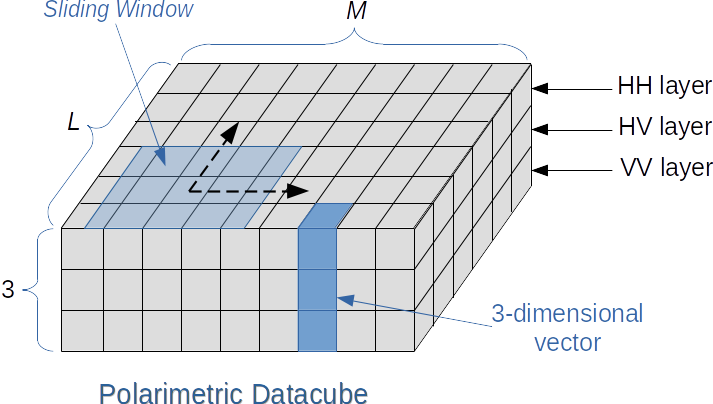
Figure 1: Schematic representation of a polarimetric SAR image as a datacube and sliding window used to obtain data under test.

A multipolarization SAR sensor generates an image (datacube) where each pixel is represented by a vector whose entries are the complex returns corresponding to the different polarimetric channels. Here, we assume that the medium is reciprocal allowing to deal with the three polarimetric channels HH, HV, and VV [10]. Let us denote by $L$ and $M$ the numbers of pixels along the vertical and horizontal dimensions of the polarimetric image, respectively, then, the sensor provides a datacube of size $L\times M\times 3$ (see Figure 1). Now, the set of vectors under test is selected using a sliding window that moves over the image and contains $K$ statistically independent random vectors ${\mbox{\boldmath$z$}}_{k}\in{\mathds{C}}^{3\times 1}$, $k=1,\ldots,K$, such that ${\mbox{\boldmath$z$}}_{k}\sim\mbox{$\mathcal{C}$}\mbox{$\mathcal{N}$}_{3}({\mbox{\boldmath$0$}},{\mbox{\boldmath$M$}}_{k})$, with ${\mbox{\boldmath$M$}}_{k}\in{\mathds{C}}^{3\times 3}$, $k=1,\ldots,K$, the positive definite unknown PCM. Moreover, the latter exhibits specific configurations according to the scattering mechanisms in play [16, 10]. Specifically, given the $k$th vector, the polarimetric structure takes on the following forms:

• in the presence of a reciprocal medium, we have that

  $${{\mbox{\boldmath$M$}}}_{k}=\begin{bmatrix}c_{hhhh}&c_{hhhv}&c_{hhvv}\\ c^{*}_{hhhv}&c_{hvhv}&c_{hvvv}\\ c^{*}_{hhvv}&c^{*}_{hvvv}&c_{vvvv}\end{bmatrix}={\mbox{\boldmath$C$}}_{1};$$ (1)

• in the presence of a reflection symmetry with respect to a vertical plane, the structure becomes

  $${{\mbox{\boldmath$M$}}}_{k}=\begin{bmatrix}c_{hhhh}&0&c_{hhvv}\\ 0&c_{hvhv}&0\\ c_{hhvv}^{*}&0&c_{vvvv}\end{bmatrix}={\mbox{\boldmath$C$}}_{2};$$ (2)

• when a rotation symmetry is present, we can write

  $${{\mbox{\boldmath$M$}}}_{k}=\begin{bmatrix}c_{hhhh}&c_{hhhv}&c_{hhvv}\\ -c_{hhhv}&c_{hvhv}&c_{hhhv}\\ c_{hhvv}&-c_{hhhv}&c_{hhhh}\end{bmatrix}={\mbox{\boldmath$C$}}_{3},$$ (3)

  where ${\mathfrak{R}e}\{c_{hhhv}\}=0$, $c_{hhvv}\in{\mathds{R}}$ and $c_{hvhv}=(c_{hhhh}-c_{hhvv})/2$;

• in the case of azimuth symmetry, it is given by

  $${{\mbox{\boldmath$M$}}}_{k}=\begin{bmatrix}c_{hhhh}&0&c_{hhvv}\\ 0&c_{hvhv}&0\\ c_{hhvv}&0&c_{hhhh}\end{bmatrix}={\mbox{\boldmath$C$}}_{4},$$ (4)

  where $c_{hhvv}\in{\mathds{R}}$ and $c_{hvhv}=(c_{hhhh}-c_{hhvv})/2$.

It turns out that within the sliding window containing the vectors under test, several situations may occur according to the involved structures. Specifically, the PCM can remain unaltered within the sliding window or at least two different forms appear within the window.

To be more precise, we are interested in distinguishing the case ${\mbox{\boldmath$M$}}_{1}=\ldots={\mbox{\boldmath$M$}}_{K}\in\mbox{$\mathcal{C}$}=\{{\mbox{\boldmath$C$}}_{1},\ldots,{\mbox{\boldmath$C$}}_{4}\}$ from different configurations where the pixels are characterized by at least two PCMs. This problem can be formulated in terms of a multiple hypothesis test consisting of one null hypothesis and several alternative hypotheses, namely as

$$\!\!\!\begin{cases}H_{0}:&\!\!\!\!\!\!\displaystyle{\mbox{\boldmath$z$}}_{k}\sim\mbox{$\mathcal{C}$}\mbox{$\mathcal{N}$}_{3}({\mbox{\boldmath$0$}},{\mbox{\boldmath$C$}}_{i_{0}}),i_{0}\in\{1,\ldots,4\},\\ H_{{1,1}}:&\!\!\!\!\!\!\begin{cases}{\mbox{\boldmath$z$}}_{k}\sim\mbox{$\mathcal{C}$}\mbox{$\mathcal{N}$}_{3}({\mbox{\boldmath$0$}},{\mbox{\boldmath$C$}}_{i_{0}}),k\in\Omega_{1}\subset\Omega,\\ {\mbox{\boldmath$z$}}_{k}\sim\mbox{$\mathcal{C}$}\mbox{$\mathcal{N}$}_{3}({\mbox{\boldmath$0$}},{\mbox{\boldmath$C$}}_{i_{1}}),k\in\Omega_{2}=\Omega\setminus\Omega_{1},\\ i_{0}<i_{1},i_{0},i_{1}\in\{1,\ldots,4\},\end{cases}\\ H_{{1,2}}:&\!\!\!\!\!\!\begin{cases}{\mbox{\boldmath$z$}}_{k}\sim\mbox{$\mathcal{C}$}\mbox{$\mathcal{N}$}_{3}({\mbox{\boldmath$0$}},{\mbox{\boldmath$C$}}_{i_{0}}),k\in\Omega_{1}\subset\Omega,\\ {\mbox{\boldmath$z$}}_{k}\sim\mbox{$\mathcal{C}$}\mbox{$\mathcal{N}$}_{3}({\mbox{\boldmath$0$}},{\mbox{\boldmath$C$}}_{i_{1}}),k\in\Omega_{2}\subset\Omega\setminus\Omega_{1},\\ {\mbox{\boldmath$z$}}_{k}\sim\mbox{$\mathcal{C}$}\mbox{$\mathcal{N}$}_{3}({\mbox{\boldmath$0$}},{\mbox{\boldmath$C$}}_{i_{2}}),k\in\Omega_{3}=\Omega\setminus\{\Omega_{1}\cup\Omega_{2}\},\\ i_{0}<i_{1}<i_{2},i_{0},i_{1},i_{2}\in\{1,\ldots,4\},\end{cases}\\ H_{{1,3}}:&\!\!\!\!\!\!\begin{cases}{\mbox{\boldmath$z$}}_{k}\sim\mbox{$\mathcal{C}$}\mbox{$\mathcal{N}$}_{3}({\mbox{\boldmath$0$}},{\mbox{\boldmath$C$}}_{1}),k\in\Omega_{1}\subset\Omega,\\ {\mbox{\boldmath$z$}}_{k}\sim\mbox{$\mathcal{C}$}\mbox{$\mathcal{N}$}_{3}({\mbox{\boldmath$0$}},{\mbox{\boldmath$C$}}_{2}),k\in\Omega_{2}\subset\Omega\setminus\Omega_{1},\\ {\mbox{\boldmath$z$}}_{k}\sim\mbox{$\mathcal{C}$}\mbox{$\mathcal{N}$}_{3}({\mbox{\boldmath$0$}},{\mbox{\boldmath$C$}}_{3}),k\in\Omega_{3}\subset\Omega\setminus\{\Omega_{1}\cup\Omega_{2}\},\\ {\mbox{\boldmath$z$}}_{k}\sim\mbox{$\mathcal{C}$}\mbox{$\mathcal{N}$}_{3}({\mbox{\boldmath$0$}},{\mbox{\boldmath$C$}}_{4}),k\in\Omega_{4}=\Omega\setminus\{\Omega_{1}\cup\Omega_{2}\cup\Omega_{3}\},\end{cases}\end{cases}$$ (5)

where $\Omega=\{1,\ldots,K\}$ and the $\Omega_{l}$s are unknown (except for $\Omega_{i+1}$ under $H_{1,i}$). The PDF of ${\mbox{\boldmath$Z$}}=[{\mbox{\boldmath$z$}}_{1},\ldots,{\mbox{\boldmath$z$}}_{K}]$ under $H_{0}$ is given by

$$p_{0}({\mbox{\boldmath$Z$}};{\mbox{\boldmath$C$}}_{i_{0}})=\frac{\exp\left\{-\mbox{\rm Tr}\,\left[{\mbox{\boldmath$C$}}_{i_{0}}^{-1}{\mbox{\boldmath$Z$}}{\mbox{\boldmath$Z$}}^{\dagger}\right]\right\}}{\pi^{3K}\left[\det\left({\mbox{\boldmath$C$}}_{i_{0}}\right)\right]^{K}},$$ (6)

whereas that under $H_{1,m}$, $m=1,\ldots,3$, can be written as

$$p_{1,m}({\mbox{\boldmath$Z$}};{\mbox{\boldmath$C$}}_{i_{0}},\ldots,{\mbox{\boldmath$C$}}_{i_{m}})\\ =\prod_{l=0}^{m}\prod_{k\in\Omega_{l+1}}\frac{\exp\left\{-\mbox{\rm Tr}\,\left[{\mbox{\boldmath$C$}}_{i_{l}}^{-1}{\mbox{\boldmath$z$}}_{k}{\mbox{\boldmath$z$}}_{k}^{\dagger}\right]\right\}}{\pi^{3}\left[\det({\mbox{\boldmath$C$}}_{i_{l}})\right]}$$ (7)

with the constraints

$$\bigcup_{l=0}^{m}\Omega_{l+1}=\Omega\quad\mbox{and}\quad\Omega_{i}\cap\Omega_{j}=\emptyset,\ i\neq j.$$ (8)

For future reference, it is also useful to define the sets

$$\mbox{$\mathcal{A}$}_{m}=\{i_{0},\ldots,i_{m}\}\subseteq\{1,\ldots,4\},\ m=0,\ldots,3,$$ (9)

and denote by ${\mbox{\boldmath$\theta$}}_{0}(\mbox{$\mathcal{A}$}_{0})$ and ${\mbox{\boldmath$\theta$}}_{1}(\mbox{$\mathcal{A}$}_{m})$ the unknown parameters under $H_{0}$, given $\mbox{$\mathcal{A}$}_{0}$, and under $H_{1,m}$, given $\mbox{$\mathcal{A}$}_{m}$, respectively.

III Detection Architecture Designs

In this section, we provide some important remarks that are preparatory to the subsequent derivations and motivate the design choices. As specified below, the adopted decision rules rely on the LLRT where the unknown parameters are replaced by suitable estimates. However, implementation of such a strategy for the problem at hand requires to circumvent two main drawbacks.

First of all, under $H_{1,m}$, the partition $\left\{\Omega_{1},\ldots,\Omega_{m+1}\right\}$ of the pixels of the sliding window is not known. As a consequence, application of the MLA to obtain the parameter estimates would be a formidable task: we should consider all the combinations of $m+1$ PCM structures over the available options, namely ${4}\choose{m+1}$, and for each of them the different partitions of $\Omega$ into $m+1$ subsets. Therefore, in what follows, we propose two alternative solutions that abstain from the computation of all the possible partitions of $\Omega$. These alternatives rely on the fact that, from an operating point of view, partitioning $\Omega$ is tantamount to labeling its elements. Therefore, we can follow the lead of [17] and introduce $K$ IID hidden discrete random variables that are representative of the labels associated with the ${\mbox{\boldmath$z$}}_{k}$s under $H_{1,m}$ and $\mbox{$\mathcal{A}$}_{m}=\{i_{0},\ldots,i_{m}\}\subseteq\{1\ldots,4\}$. In fact, such random variables take on values in $\mbox{$\mathcal{A}$}_{m}$. Then, we apply the EM algorithm [13] to estimate the unknown parameters. The herein proposed estimation procedures differ from each other in the way such hidden random variables are defined and used to build up the LLRT, a point better specified at the end of this section.

The second drawback of implementing a plain LLRT is originated by the fact that the elements of $\mathcal{C}$ are characterized by different numbers of unknowns. Thus, not only a balanced comparison of the hypotheses, but also of the different $\mbox{$\mathcal{A}$}_{m}$s, given $m$ (i.e., given the hypothesis), requires introducing adequate penalty factors. To be more quantitative, we observe that the number $n_{i}$ of unknown parameters associated with ${\mbox{\boldmath$C$}}_{i}$, $i=1,\ldots,4$, is given by

$$n_{i}=\begin{cases}9&\mbox{if }i=1,\\ 5&\mbox{if }i=2,\\ 3&\mbox{if }i=3,\\ 2&\mbox{if }i=4.\end{cases}$$ (10)

Accordingly, the number of unknowns associated with $\mbox{$\mathcal{A}$}_{m}=\{i_{0},\ldots,i_{m}\}$ can be computed as $u\left(\mbox{$\mathcal{A}$}_{m}\right)=\sum_{j=0}^{m}n_{i_{j}}$.

With the above remarks in mind, we devise decision schemes for problem (5) exploiting a penalized LLRT [18]. As a first step towards the introduction of such a penalized LLRT, we denote by $\widehat{{\mbox{\boldmath$\theta$}}}_{0}(\mbox{$\mathcal{A}$}_{0})$ ($\widehat{{\mbox{\boldmath$\theta$}}}_{1}(\mbox{$\mathcal{A}$}_{m})$) the estimate of the unknown parameters related to $H_{0}$ and $\mbox{$\mathcal{A}$}_{0}$ ($H_{1,m}$ and $\mbox{$\mathcal{A}$}_{m}$). Similarly, $\widehat{{\mbox{\boldmath$\theta$}}}_{1}(\mbox{$\mathcal{A}$}_{\widehat{m}})$ is the estimate of the unknown parameters associated with $H_{1,\widehat{m}}$ and $\mbox{$\mathcal{A}$}_{\widehat{m}}$. For the moment we leave aside the description of the estimation procedures, which will be the object of the next subsections, and introduce the general structure of the penalized LLRT

$$\max_{m\in\{1,2,3\}}\max_{\mbox{$\mathcal{A}$}_{m}}\left[\log g_{1}\left({\mbox{\boldmath$Z$}};\widehat{{\mbox{\boldmath$\theta$}}}_{1}\left(\mbox{$\mathcal{A}$}_{m}\right)\right)-h_{1}\left(\mbox{$\mathcal{A}$}_{m}\right)\right]$$

$$-\max_{\mbox{$\mathcal{A}$}_{0}}\left[\log g_{0}\left({\mbox{\boldmath$Z$}};\widehat{{\mbox{\boldmath$\theta$}}}_{0}\left(\mbox{$\mathcal{A}$}_{0}\right)\right)-h_{0}\left(\mbox{$\mathcal{A}$}_{0}\right)\right]\mbox{$\begin{array}[]{c}\stackrel{{\scriptstyle\stackrel{{\scriptstyle\textstyle H_{1,\widehat{m}}}}{{\textstyle>}}}}{{\stackrel{{\scriptstyle\textstyle<}}{{\textstyle H_{0}}}}}\end{array}$}\eta,$$ (12)

where

$$\widehat{m}=\operatorname*{arg\,max}_{m\in\{1,2,3\}}\left\{\max_{\mbox{$\mathcal{A}$}_{m}}\left[\log g_{1}\left({\mbox{\boldmath$Z$}};\widehat{{\mbox{\boldmath$\theta$}}}_{1}\left(\mbox{$\mathcal{A}$}_{m}\right)\right)-h_{1}\left(\mbox{$\mathcal{A}$}_{m}\right)\right]\right\},$$

$g_{0}\left({\mbox{\boldmath$Z$}};{\mbox{\boldmath$\theta$}}_{0}\left(\mbox{$\mathcal{A}$}_{0}\right)\right)=p_{0}({\mbox{\boldmath$Z$}};{\mbox{\boldmath$C$}}_{i_{0}})$, $g_{1}\left({\mbox{\boldmath$Z$}};{\mbox{\boldmath$\theta$}}_{1}\left(\mbox{$\mathcal{A}$}_{m}\right)\right)$ denotes the PDF of the observables under $H_{1,m}$ and $\mbox{$\mathcal{A}$}_{m}$, that will be specified by subsequent sections, $h_{1}\left(\mbox{$\mathcal{A}$}_{m}\right)$, $m=1,2,3$, is a penalty term accounting for the number of unknown parameters related to $H_{1,m}$ and $\mbox{$\mathcal{A}$}_{m}$, $h_{0}\left(\mbox{$\mathcal{A}$}_{0}\right)$ is a penalty term accounting for the number of unknown parameters related to $H_{0}$ and $\mbox{$\mathcal{A}$}_{0}$, and $\eta$ is the detection threshold to be set according to the probability of false alarm ($P_{fa}$). The penalty terms can be written as $h_{1}(\mbox{$\mathcal{A}$}_{m})=\gamma\left(u\left(\mbox{$\mathcal{A}$}_{m}\right)+m+1\right)$ and $h_{0}(\mbox{$\mathcal{A}$}_{0})=\gamma u\left(\mbox{$\mathcal{A}$}_{0}\right)$ where we recall that $u\left(\mbox{$\mathcal{A}$}_{m}\right)$ is the number of unknown real-valued parameters associated with $\mbox{$\mathcal{A}$}_{m}$, $m+1$ is the number of unknowns related to the probability mass function (PMF) of the hidden discrete random variables (such random variables take on values in $\mbox{$\mathcal{A}$}_{m}$), and $\gamma$ is a factor borrowed from the MOS rules [15] as the Akaike Information Criterion (AIC), the Generalized Information Criterion (GIC), and the Bayesian Information Criterion (BIC), i.e.,

$$\gamma=\begin{cases}1,&\mbox{for AIC-based Detector (AIC-D)},\\ \log(6K)/2,&\mbox{for BIC-based Detector (BIC-D)},\\ (1+\rho)/2,\ \rho>1,&\mbox{for GIC-based Detector (GIC-D)}.\end{cases}$$ (13)

It is important to stress that, under $H_{1,m}$ and $\mbox{$\mathcal{A}$}_{m}$, $u\left(\mbox{$\mathcal{A}$}_{m}\right)$ is obtained by partitioning the data set into $m+1$ subsets, associating with them specific structures, and summing the respective number of unknown parameters. The cardinality of each subset along with the coordinates of the vectors within it are also unknowns, but they are independent of $\mbox{$\mathcal{A}$}_{m}$ and, hence, irrelevant to the decision process.

It still remain to show how to estimate ${\mbox{\boldmath$\theta$}}_{0}(\mbox{$\mathcal{A}$}_{0})$ and ${\mbox{\boldmath$\theta$}}_{1}(\mbox{$\mathcal{A}$}_{m})$. As previously anticipated, we will follow the lead of [17] and introduce $K$ independent and identically distributed hidden discrete random variables that “specify the characterization” of the ${\mbox{\boldmath$z$}}_{k}$s. Then, we apply the EM algorithm [13] to estimate the unknown parameters. The herein proposed estimation procedures differ from each other in the way such hidden random variables are defined and used to build up the LLRT under $H_{1,m}$.

The first procedure assumes that under $H_{1,m}$ the hidden random variables, $c_{k,m}$ say, have alphabet $\mbox{$\mathcal{A}$}_{m}=\{i_{0},\ldots,i_{m}\}\subseteq\{1\ldots,4\}$ with PMF

$$\begin{cases}P(c_{k,m}=l)=P_{l,m},\ l\in\mbox{$\mathcal{A}$}_{m},\\ \displaystyle\sum_{l\in{\mathcal{A}}_{m}}P_{l,m}=1,\end{cases}$$ (14)

and that when $c_{k,m}=l$, $l\in\mbox{$\mathcal{A}$}_{m}$, then ${\mbox{\boldmath$M$}}_{k}={\mbox{\boldmath$C$}}_{l}$. Therefore, we can write the PDF of ${\mbox{\boldmath$z$}}_{k}$ under $H_{1,m}$ as [17]

$$f_{1,m}({\mbox{\boldmath$z$}}_{k};{\mbox{\boldmath$\theta$}}_{1}(\mbox{$\mathcal{A}$}_{m}))=\sum_{l\in{\mathcal{A}}_{m}}P_{l,m}f({\mbox{\boldmath$z$}}_{k};{\mbox{\boldmath$C$}}_{l}),$$ (15)

where $f({\mbox{\boldmath$z$}}_{k};{\mbox{\boldmath$C$}}_{l})$ is the PDF of ${\mbox{\boldmath$z$}}_{k}\sim\mbox{$\mathcal{C}$}\mbox{$\mathcal{N}$}({\mbox{\boldmath$0$}},{\mbox{\boldmath$C$}}_{l})$. The above PDF will be used in place of the original PDF to form the LLRT. Notice that ${\mbox{\boldmath$\theta$}}_{1}(\mbox{$\mathcal{A}$}_{m})$ depends on the specific choice for the alphabet of the hidden random variables. As a matter of fact, for each alternative hypothesis, each of the ${4}\choose{m+1}$ combinations of the PCM structures identifies an alphabet configuration. Thus, we come up with $6$, $4$, and $1$ different alphabet configurations under $H_{1,1}$, $H_{1,2}$, and $H_{1,3}$, respectively. Nevertheless, as we will show in the next subsections, these configurations can be handled without a dramatic increase of the computational requirements.

The second approach does not account for the hypotheses $H_{1,1}$, $H_{1,2}$, and $H_{1,3}$ to set the number of classes but simply considers all classes. As consequence, the hidden random variables, $c_{k}$ say, share the same alphabet $\mbox{$\mathcal{A}$}=\{1,2,3,4\}$ and PMF $P(c_{k}=l)=P_{l}$, $l\in\mbox{$\mathcal{A}$}$. The LLRT under $H_{1,m}$ is formed by selecting the $m+1$ most probable PCM structures and modifying (15) according to the selected structures.

In the next subsections, we describe in the detail these procedures that are based upon the EM algorithm.

III-A First EM-based Estimation Strategy

Let us assume that under $H_{1,m}$, $m=1,2,3$, equation (15) holds true and focus on problem (5). Now, given a configuration for $\mbox{$\mathcal{A}$}_{m}$, the log-likelihood of $Z$ is given by

$$\log g_{1}\left({\mbox{\boldmath$Z$}};{\mbox{\boldmath$\theta$}}_{1}\left(\mbox{$\mathcal{A}$}_{m}\right)\right)=\sum_{k=1}^{K}\log\sum_{l\in{\mathcal{A}}_{m}}P_{l,m}f({\mbox{\boldmath$z$}}_{k};{\mbox{\boldmath$C$}}_{l}).$$ (16)

The application of the EM algorithm consists of the E-step that leads to [17, 19]

$$q_{k}^{(h-1)}(l,m)=\frac{f({\mbox{\boldmath$z$}}_{k};\widehat{{\mbox{\boldmath$C$}}}_{l}^{(h-1)})\widehat{P}_{l,m}^{(h-1)}}{\displaystyle\sum_{n\in{\mathcal{A}}_{m}}f({\mbox{\boldmath$z$}}_{k};\widehat{{\mbox{\boldmath$C$}}}_{n}^{(h-1)})\widehat{P}_{n,m}^{(h-1)}},\quad l\in\mbox{$\mathcal{A}$}_{m},$$ (17)

where $\widehat{P}_{l,m}^{(h-1)}$, $l\in\mbox{$\mathcal{A}$}_{m}$, and $\widehat{{\mbox{\boldmath$C$}}}_{n}^{(h-1)}$, $n\in\mbox{$\mathcal{A}$}_{m}$, are the available estimates at the $(h-1)$th step, and of the M-step requiring to solve the following joint optimization problem

$$\max_{{\bf p}_{m}}\displaystyle\max_{{\bf C}_{l}\atop l\in{\mathcal{A}}_{m}}\bigg{\{}\sum_{k=1}^{K}\sum_{l\in{\mathcal{A}}_{m}}q_{k}^{(h-1)}(l,m)[-\log\det({\mbox{\boldmath$C$}}_{l})\\ -\mbox{\rm Tr}\,({\mbox{\boldmath$C$}}_{l}^{-1}{\mbox{\boldmath$z$}}_{k}{\mbox{\boldmath$z$}}_{k}^{\dagger})]-\sum_{k=1}^{K}\sum_{l\in{\mathcal{A}}_{m}}q_{k}^{(h-1)}(l,m)\log P_{l,m}\bigg{\}},$$ (18)

where $\mbox{\boldmath$p$}_{m}=[P_{i_{0},m},\ldots,P_{i_{m},m}]^{T}\in{\mathds{R}}^{(m+1)\times 1}$.

It is not difficult to show that the maximization with respect to $\mbox{\boldmath$p$}_{m}$, accomplished under the constraint

$$\sum_{l\in\mbox{$\mathcal{A}$}_{m}}P_{l,m}=1,$$ (19)

returns the following stationary points

$$\widehat{P}_{l,m}^{(h)}=\frac{1}{K}\sum_{k=1}^{K}q_{k}^{(h-1)}(l,m),\quad l\in\mbox{$\mathcal{A}$}_{m}.$$ (20)

On the other hand, the maximization with respect to ${\mbox{\boldmath$C$}}_{l}$ for a given $\bar{l}\in\mbox{$\mathcal{A}$}_{m}$ implies

$$\max_{{\mbox{\boldmath$C$}}_{\bar{l}}}\sum\limits_{k=1}^{K}q_{k}^{(h-1)}(\bar{l},m)\left[-\log\det({\mbox{\boldmath$C$}}_{\bar{l}})-\mbox{\rm Tr}\,\left({\mbox{\boldmath$C$}}_{\bar{l}}^{-1}{\mbox{\boldmath$z$}}_{k}{\mbox{\boldmath$z$}}_{k}^{{\dagger}}\right)\right].$$ (21)

Let us solve the above problem for each possible value taken on by $\bar{l}$. To this end, notice that when $\bar{l}=1$, we have that

$$\sum_{k=1}^{K}q_{k}^{(h-1)}(1,m)\left[-\log\det({\mbox{\boldmath$C$}}_{1})-\mbox{\rm Tr}\,\left({\mbox{\boldmath$C$}}_{1}^{-1}{\mbox{\boldmath$z$}}_{k}{\mbox{\boldmath$z$}}_{k}^{{\dagger}}\right)\right]$$

$$=q^{(h-1)}(1,m)\left\{\log\det({\mbox{\boldmath$C$}}_{1}^{-1})-\mbox{\rm Tr}\,\left[{\mbox{\boldmath$C$}}_{1}^{-1}{\mbox{\boldmath$S$}}_{q}(1,m)^{(h-1)}\right]\right\},$$ (22)

where $q^{(h-1)}(1,m)=\sum_{k=1}^{K}q_{k}^{(h-1)}(1,m)$, ${\mbox{\boldmath$S$}}_{q}(1,m)^{(h-1)}=\sum_{k=1}^{K}q_{k}^{(h-1)}(1,m){\mbox{\boldmath$z$}}_{k}{\mbox{\boldmath$z$}}_{k}^{\dagger}/q^{(h-1)}(1,m)$. It follows that

$$\max_{{\mbox{\boldmath$C$}}_{1}}\log\det({\mbox{\boldmath$C$}}_{1}^{-1})-\mbox{\rm Tr}\,\left[{\mbox{\boldmath$C$}}_{1}^{-1}{\mbox{\boldmath$S$}}_{q}(1,m)^{(h-1)}\right]$$ (23)

is tantamount to maximize

$$\log\det\left({\mbox{\boldmath$C$}}_{1}^{-1}{\mbox{\boldmath$S$}}_{q}(1,m)^{(h-1)}\right)-\log\det\left({\mbox{\boldmath$S$}}_{q}(1,m)^{(h-1)}\right)\\ -\mbox{\rm Tr}\,\left[{\mbox{\boldmath$C$}}_{1}^{-1}{\mbox{\boldmath$S$}}_{q}(1,m)^{(h-1)}\right].$$ (24)

The maximizer can be obtained resorting to the following inequality [20]

$$\log\det({\mbox{\boldmath$A$}})\leq\mbox{\rm Tr}\,[{\mbox{\boldmath$A$}}]-3,$$ (25)

where $A$ is any matrix with nonnegative eigenvalues, and, hence, it follows that

$$\widehat{{\mbox{\boldmath$C$}}}_{1}^{(h)} =\operatorname*{arg\,max}_{{\mbox{\boldmath$C$}}_{1}}\sum\limits_{k=1}^{K}q_{k}^{(h-1)}(1,m)$$

$$\times\left[-\log\det({\mbox{\boldmath$C$}}_{1})-\mbox{\rm Tr}\,\left({\mbox{\boldmath$C$}}_{1}^{-1}{\mbox{\boldmath$z$}}_{k}{\mbox{\boldmath$z$}}_{k}^{{\dagger}}\right)\right]$$

$$=\frac{\displaystyle\sum_{k=1}^{K}q_{k}^{(h-1)}(1,m){\mbox{\boldmath$z$}}_{k}{\mbox{\boldmath$z$}}_{k}^{\dagger}}{\displaystyle\sum_{k=1}^{K}q_{k}^{(h-1)}(1,m)}.$$

Now, assume that $\bar{l}=2$ and let $U$ be the unitary matrix defined in Lemma 3.1 of [11], then

$${\mbox{\boldmath$U$}}{\mbox{\boldmath$C$}}_{2}{\mbox{\boldmath$U$}}^{\dagger}=\begin{bmatrix}{\mbox{\boldmath$A$}}&{\mbox{\boldmath$0$}}\\ {\mbox{\boldmath$0$}}&d\end{bmatrix},$$ (26)

where ${\mbox{\boldmath$A$}}\in{\mathds{C}}^{2\times 2}$ is positive definite and $d>0$. It follows that problem (21) can be recast as

$$\max_{{\mbox{\boldmath$A$}}}\displaystyle\max_{d>0}\sum_{k=1}^{K}q_{k}^{(h-1)}(2,m)\left[-\log\det({\mbox{\boldmath$A$}})-\log d\right.\\ \left.-{\mbox{\boldmath$z$}}^{\dagger}_{k,1}{\mbox{\boldmath$A$}}^{-1}{\mbox{\boldmath$z$}}_{k,1}-|z_{k,2}|^{2}d^{-1}\right]$$ (27)

where ${\mbox{\boldmath$U$}}{\mbox{\boldmath$z$}}_{k}=[{\mbox{\boldmath$z$}}_{k,1}^{T}\ z_{k,2}]^{T}$ with ${\mbox{\boldmath$z$}}_{k,1}\in{\mathds{C}}^{2\times 1}$ and $z_{k,2}\in{\mathds{C}}$. Now, observe that

$$\lim_{d\rightarrow 0\atop d\rightarrow+\infty}\left[-\sum_{k=1}^{K}q_{k}^{(h-1)}(2,m)(\log d+|z_{k,2}|^{2}d^{-1})\right]=-\infty.$$ (28)

Thus, the stationary points over $d>0$ can be found by setting to zero the first derivative with respect to $d$ of the argument of (27), to obtain

$$-\sum_{k=1}^{K}\frac{{q}_{k}^{(h-1)}(2,m)}{d}+\frac{1}{d^{2}}\sum_{k=1}^{K}{q}_{k}^{(h-1)}(2,m)|z_{k,2}|^{2}=0.$$ (29)

Thus, the update of the estimate of $d$ is

$$\widehat{d}^{(h)}=\frac{\sum\limits_{k=1}^{K}{q}_{k}^{(h-1)}(2,m)|{z}_{k,2}|^{2}}{\sum\limits_{k=1}^{K}{q}_{k}^{(h-1)}(2,m)}.$$ (30)

As for $A$, let us consider

$$\max_{{\mbox{\boldmath$A$}}}\sum_{k=1}^{K}q_{k}^{(h-1)}(2,m)\left[-\log\det({\mbox{\boldmath$A$}})-{\mbox{\boldmath$z$}}^{\dagger}_{k,1}{\mbox{\boldmath$A$}}^{-1}{\mbox{\boldmath$z$}}_{k,1}\right],$$ (31)

which can be recast as

$$\displaystyle\max_{{\mbox{\boldmath$A$}}}q^{(h-1)}(2,m)\log\det({\mbox{\boldmath$A$}}^{-1})-\mbox{\rm Tr}\,\left[{\mbox{\boldmath$A$}}^{-1}{\mbox{\boldmath$S$}}(2,m)^{(h-1)}\right],$$

$$\Rightarrow\displaystyle\max_{{\mbox{\boldmath$A$}}}\log\det\left[{\mbox{\boldmath$A$}}^{-1}{{\mbox{\boldmath$S$}}(2,m)^{(h-1)}}/{q^{(h-1)}(2,m)}\right]$$

$$\quad-\mbox{\rm Tr}\,\left[{\mbox{\boldmath$A$}}^{-1}{{\mbox{\boldmath$S$}}(2,m)^{(h-1)}}/{q^{(h-1)}(2,m)}\right],$$ (32)

where $q^{(h-1)}(2,m)=\sum_{k=1}^{K}q_{k}^{(h-1)}(2,m)$ and ${\mbox{\boldmath$S$}}(2,m)^{(h-1)}=\sum_{k=1}^{K}q_{k}^{(h-1)}(2,m){\mbox{\boldmath$z$}}_{k,1}{\mbox{\boldmath$z$}}_{k,1}^{\dagger}$. Exploiting (25), the resulting maximizer for the last problem can be written as

$$\widehat{{\mbox{\boldmath$A$}}}^{(h)}=\frac{\displaystyle\sum_{k=1}^{K}{q}_{k}^{(h-1)}(2,m){\mbox{\boldmath$z$}}_{k,1}{\mbox{\boldmath$z$}}_{k,1}^{\dagger}}{\displaystyle\sum_{k=1}^{K}{q}_{k}^{(h-1)}(2,m)}.$$ (33)

As a consequence, an estimate of ${\mbox{\boldmath$C$}}_{2}$ is given by

$$\widehat{{\mbox{\boldmath$C$}}}_{2}^{(h)}={\mbox{\boldmath$U$}}^{\dagger}\begin{bmatrix}\widehat{{\mbox{\boldmath$A$}}}^{(h)}&{\mbox{\boldmath$0$}}\\ {\mbox{\boldmath$0$}}&\widehat{d}^{(h)}\end{bmatrix}{\mbox{\boldmath$U$}}.$$ (34)

The next case is $\bar{l}=3$. Notice that matrix ${\mbox{\boldmath$C$}}_{3}$ can be suitably manipulated by applying the transformations represented by matrices $E$, $T$, and $V$ defined in Lemma 3.1 of [11], namely

$${\mbox{\boldmath$V$}}{\mbox{\boldmath$E$}}{\mbox{\boldmath$T$}}{\mbox{\boldmath$C$}}_{3}{\mbox{\boldmath$T$}}^{{\dagger}}{\mbox{\boldmath$E$}}{\mbox{\boldmath$V$}}^{{\dagger}}=\begin{bmatrix}a&{\mbox{\boldmath$0$}}\\ {\mbox{\boldmath$0$}}&{\mbox{\boldmath$B$}}\end{bmatrix},$$ (35)

where $a>0$ and ${\mbox{\boldmath$B$}}\in{\mathds{R}}^{2\times 2}$ is centrosymmetric. The objective function can be accordingly expressed as follows

$$\max_{a}\displaystyle\max_{{\mbox{\boldmath$B$}}}\sum_{k=1}^{K}q_{k}^{(h-1)}(3,m)\left[-\log a-\log\det({\mbox{\boldmath$B$}})\right.\\ \left.-\frac{|x_{k,1}|^{2}}{a}-{\mbox{\boldmath$x$}}_{k,2}^{\dagger}{\mbox{\boldmath$B$}}^{-1}{\mbox{\boldmath$x$}}_{k,2}\right],$$ (36)

where ${\mbox{\boldmath$V$}}{\mbox{\boldmath$E$}}{\mbox{\boldmath$T$}}{\mbox{\boldmath$z$}}_{k}=[x_{k,1}\ {\mbox{\boldmath$x$}}_{k,2}^{T}]^{T}$ with $x_{k,1}\in{\mathds{C}}$ and ${\mbox{\boldmath$x$}}_{k,2}\in{\mathds{C}}^{2\times 1}$. Now, since $B$ is centrosymmetric, the equality ${\mbox{\boldmath$B$}}^{-1}=\left({\mbox{\boldmath$B$}}^{-1}+{\mbox{\boldmath$J$}}{\mbox{\boldmath$B$}}^{-1}{\mbox{\boldmath$J$}}\right)/{2}$ holds and (36) can be written as

$$\max_{a}\max_{{\mbox{\boldmath$B$}}}\sum\limits_{k=1}^{K}q_{k}^{(h-1)}(3,m)\left[-\log a-\log\det({\mbox{\boldmath$B$}})\right.\\ \left.-\frac{|x_{k,1}|^{2}}{a}-\frac{1}{2}\mbox{\rm Tr}\,\left[{\mbox{\boldmath$B$}}^{-1}\left({\mbox{\boldmath$x$}}_{k,2}{\mbox{\boldmath$x$}}_{k,2}^{{\dagger}}+{\mbox{\boldmath$J$}}{\mbox{\boldmath$x$}}_{k,2}{\mbox{\boldmath$x$}}_{k,2}^{{\dagger}}{\mbox{\boldmath$J$}}\right)\right]\right].$$ (37)

Following the same line of reasoning as for the estimation of $d$ and $A$, it is possible to show that the estimate of $a$ is

$$\widehat{a}^{(h)}=\frac{\sum\limits_{k=1}^{K}{q}_{k}^{(h-1)}(3,m)|x_{k,1}|^{2}}{\displaystyle\sum_{k=1}^{K}{q}_{k}^{(h-1)}(3,m)},$$ (38)

whereas, using (25), the estimate of $B$ has the following expression

$$\widehat{{\mbox{\boldmath$B$}}}^{(h)}=\frac{1}{2}\frac{\displaystyle\sum_{k=1}^{K}{q}_{k}^{(h-1)}(3,m)\left({\mbox{\boldmath$x$}}_{k,2}{\mbox{\boldmath$x$}}_{k,2}^{\dagger}+{\mbox{\boldmath$J$}}{\mbox{\boldmath$x$}}_{k,2}{\mbox{\boldmath$x$}}_{k,2}^{\dagger}{\mbox{\boldmath$J$}}\right)}{\displaystyle\sum_{k=1}^{K}{q}_{k}^{(h-1)}(3,m)}.$$ (39)

Gathering the above results, we obtain

$$\widehat{{\mbox{\boldmath$C$}}}_{3}^{(h)}={\mbox{\boldmath$T$}}^{\dagger}{\mbox{\boldmath$E$}}^{-1}{\mbox{\boldmath$V$}}^{{\dagger}}\begin{bmatrix}\widehat{a}^{(h)}&{\mbox{\boldmath$0$}}\\ {\mbox{\boldmath$0$}}&\widehat{{\mbox{\boldmath$B$}}}^{(h)}\end{bmatrix}{\mbox{\boldmath$V$}}{\mbox{\boldmath$E$}}^{-1}{\mbox{\boldmath$T$}}.$$ (40)

The final case assumes that $\bar{l}=4$ and ${\mbox{\boldmath$C$}}_{4}$ can be transformed as follows

$$\mathbf{E}\mathbf{T}{\mbox{\boldmath$C$}}_{4}\mathbf{T}^{\dagger}\mathbf{E}=\begin{bmatrix}b&0&0\\ 0&c&0\\ 0&0&c\end{bmatrix}\in\mathbb{R}^{3\times 3},$$ (41)

where $b>0$ and $c>0$. As a consequence, the optimization problem to be solved is

$$\max_{b>0}\displaystyle\max_{c>0}\sum_{k=1}^{K}q_{k}^{(h-1)}(4,m)\left[-\log b-2\log c\right.\\ \left.-\frac{|y_{k,1}|^{2}}{b}-\frac{1}{c}{\mbox{\boldmath$y$}}_{k,2}^{{\dagger}}{\mbox{\boldmath$y$}}_{k,2}\right]$$ (42)

where ${\mbox{\boldmath$E$}}{\mbox{\boldmath$T$}}{\mbox{\boldmath$z$}}_{k}=[y_{k,1}\ {\mbox{\boldmath$y$}}_{k,2}^{T}]^{T}$ with $y_{k,1}\in{\mathds{C}}$ and ${\mbox{\boldmath$y$}}_{k,2}\in{\mathds{C}}^{2\times 1}$. Now, observe that

$$\lim_{b\rightarrow 0\atop b\rightarrow+\infty}\left\{-\sum_{k=1}^{K}q_{k}^{(h-1)}(4,m)\left[\log b+\frac{|y_{k,1}|^{2}}{b}\right]\right\} =-\infty,$$ (43)

$$\lim_{c\rightarrow 0\atop c\rightarrow+\infty}\left\{-\sum_{k=1}^{K}q_{k}^{(h-1)}(4,m)\left[2\log c+\frac{1}{c}{\mbox{\boldmath$y$}}_{k,2}^{{\dagger}}{\mbox{\boldmath$y$}}_{k,2}\right]\right\} =-\infty,$$ (44)

and, hence, setting to zero the first derivatives of the above functions with respect to $b$ and $c$, respectively, it is not difficult to show that

$$\widehat{b}^{(h)}=\frac{\sum\limits_{k=1}^{K}{q}_{k}^{(h-1)}(4,m)|y_{k,1}|^{2}}{\sum\limits_{k=1}^{K}{q}_{k}^{(h-1)}(4,m)},$$ (45)

$$\widehat{c}^{(h)}=\frac{1}{2}\frac{\sum\limits_{k=1}^{K}{q}_{k}^{(h-1)}(4,m){\mbox{\boldmath$y$}}_{k,2}^{\dagger}{\mbox{\boldmath$y$}}_{k,2}}{\sum\limits_{k=1}^{K}{q}_{k}^{(h-1)}(4,m)}.$$ (46)

Finally, the estimate of ${\mbox{\boldmath$C$}}_{4}$ is

$$\widehat{{\mbox{\boldmath$C$}}}_{4}^{(h)}={\mbox{\boldmath$T$}}^{\dagger}{\mbox{\boldmath$E$}}^{-1}\begin{bmatrix}\widehat{b}^{(h)}&0&0\\ 0&\widehat{c}^{(h)}&0\\ 0&0&\widehat{c}^{(h)}\end{bmatrix}{\mbox{\boldmath$E$}}^{-1}{\mbox{\boldmath$T$}}.$$ (47)

The actual implementation of the EM algorithm, necessary to obtain an estimate of ${{\mbox{\boldmath$\theta$}}_{1}}(\mbox{$\mathcal{A}$}_{m})$, needs to specify the convergence criterion that can be used to terminate the iterations. In what follows, for each $\mbox{$\mathcal{A}$}_{m}$, $m=1,2,3$, we adopt the following criterion

$$\Delta\mbox{$\mathcal{L}$}_{m}(h)=\Bigg{|}\Bigg{[}\mbox{$\mathcal{L}$}_{m}\left(\widehat{{\mbox{\boldmath$\theta$}}}_{1}^{(h)}(\mbox{$\mathcal{A}$}_{m});{\mbox{\boldmath$Z$}}\right)\\ -\mbox{$\mathcal{L}$}_{m}\left(\widehat{{\mbox{\boldmath$\theta$}}}_{1}^{(h-1)}(\mbox{$\mathcal{A}$}_{m});{\mbox{\boldmath$Z$}}\right)\Bigg{]}/{\mbox{$\mathcal{L}$}_{m}\left(\widehat{{\mbox{\boldmath$\theta$}}}_{1}^{(h-1)}(\mbox{$\mathcal{A}$}_{m});{\mbox{\boldmath$Z$}}\right)}\Bigg{|}<\epsilon_{m},$$ (48)

where $\mbox{$\mathcal{L}$}_{m}(\widehat{{\mbox{\boldmath$\theta$}}}_{1}^{(h)}(\mbox{$\mathcal{A}$}_{m});{\mbox{\boldmath$Z$}})=\log g_{1}({\mbox{\boldmath$Z$}};\widehat{{\mbox{\boldmath$\theta$}}}^{(h)}_{1}\left(\mbox{$\mathcal{A}$}_{m}\right))$ (see (16)) and $\epsilon_{m}>0$ is set accounting for the requirements in terms of system reactivity.

The decision statistic of test (12) also requires to estimate the unknown parameters under $H_{0}$. The MLE of ${\mbox{\boldmath$C$}}_{i}$ is given by Proposition 3.2 of [11].

III-B Second EM-based Estimation Strategy

The second procedure builds up the term associated with $H_{1,m}$ of the left-hand side of (12) by considering the estimates obtained through the first procedure under $H_{1,3}$ only. Specifically, let us assume that $\mbox{$\mathcal{A}$}_{3}=\{1,2,3,4\}$ and, given $m$, select the $m+1$ structures corresponding to the indices of the $m+1$ highest entries of the final estimate of $\mbox{\boldmath$p$}_{3}$ that is denoted by $\widehat{\mbox{\boldmath$p$}}_{3}=\left[\widehat{P}_{1,3},\widehat{P}_{2,3},\widehat{P}_{3,3},\widehat{P}_{4,3}\right]^{T}$.

To be more formal, let us sort the $\widehat{P}_{l,3}$s in descending order, namely

$$\widehat{P}_{l_{0},3}\geq\widehat{P}_{l_{1},3}\geq\widehat{P}_{l_{2},3}\geq\widehat{P}_{l_{3},3},$$ (49)

and form the following subsets $\tilde{\mbox{$\mathcal{A}$}}_{m}=\{l_{0},\ldots,l_{m}\}$, $m=1,2,3$, along with the estimate $\tilde{{\mbox{\boldmath$\theta$}}}_{1}(\tilde{\mbox{$\mathcal{A}$}}_{m})$ that can be drawn from $\widehat{{\mbox{\boldmath$\theta$}}}_{1}(\mbox{$\mathcal{A}$}_{3})$ by picking the components corresponding to the indices $l_{0},\ldots,l_{m}$. Then, decision rule (12) becomes

$$\max_{m\in\{1,2,3\}}\left[\log g_{1}\left({\mbox{\boldmath$Z$}};\tilde{{\mbox{\boldmath$\theta$}}}_{1}\left(\tilde{\mbox{$\mathcal{A}$}}_{m}\right)\right)-h_{1}\left(\tilde{\mbox{$\mathcal{A}$}}_{m}\right)\right]$$

$$-\max_{\mbox{$\mathcal{A}$}_{0}}\left[\log g_{0}\left({\mbox{\boldmath$Z$}};\widehat{{\mbox{\boldmath$\theta$}}}_{0}\left(\mbox{$\mathcal{A}$}_{0}\right)\right)-h_{0}\left(\mbox{$\mathcal{A}$}_{0}\right)\right]\mbox{$\begin{array}[]{c}\stackrel{{\scriptstyle\stackrel{{\scriptstyle\textstyle H_{1,\widehat{m}}}}{{\textstyle>}}}}{{\stackrel{{\scriptstyle\textstyle<}}{{\textstyle H_{0}}}}}\end{array}$}\eta,$$ (51)

where

$$g_{1}\left({\mbox{\boldmath$Z$}};\tilde{{\mbox{\boldmath$\theta$}}}_{1}\left(\tilde{\mbox{$\mathcal{A}$}}_{m}\right)\right)=\sum_{k=1}^{K}\log\sum_{l\in\tilde{{\mathcal{A}}}_{m}}\widehat{P}_{l,m}f({\mbox{\boldmath$z$}}_{k};\widehat{{\mbox{\boldmath$C$}}}_{l}).$$ (52)

The estimation of the unknown parameters under $H_{0}$ is the same as that of previous subsection.

III-C Architecture Summary

According to the specific penalty term in (12), that depends on (13), and the procedure pursued to come up with the parameter estimates, we can form the following architectures:

• AIC-D coupled with procedure $1$ (AIC-D-P1) or procedure $2$ (AIC-D-P2);

• BIC-D coupled with procedure $1$ (BIC-D-P1) or procedure $2$ (BIC-D-P2);

• GIC-D coupled with procedure $1$ (GIC-D-P1) or procedure $2$ (GIC-D-P2).

Finally, regardless the estimation procedure applied to data under test, once the unknown parameters have been estimated, data classification is accomplished as follows

$${\mbox{\boldmath$z$}}_{k}\longrightarrow{\mbox{\boldmath$C$}}_{\hat{i}}\ \mbox{ if }\hat{i}=\operatorname*{arg\,max}_{l\in\widehat{{\mathcal{A}}}_{\widehat{m}}}q_{k}^{(h_{\max})}(l,\widehat{m}),$$ (53)

where $h_{\max}$ is the maximum number of EM iterations used to come up with the final parameter estimates, while $\widehat{\mbox{$\mathcal{A}$}}_{m}$ and $\widehat{m}$ are the final estimates of $\mathcal{A}$ and $m$, respectively.

IV Numerical Examples

In this section, the behaviors of the proposed architectures are assessed using synthetic data as well as real polarimetric SAR data. Specifically, the first subsection contains the performance results over simulated data obtained by means of standard Monte Carlo (MC) counting techniques, whereas in Subsection IV-B, the proposed procedures are tested using real polarimetric SAR data. For comparison purposes, we also investigate the performance of the solutions proposed in [11]. Notice that these comparisons are performed in terms of classification capabilities only, because the architectures proposed in [11] are classifiers that operate under $H_{0}$ of (5), namely, they select the most plausible PCM structure assuming that all the cells under considerations share the same covariance structure.

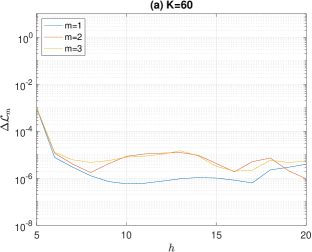
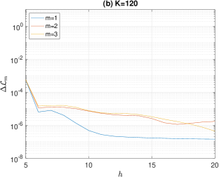
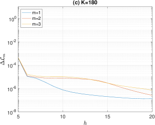
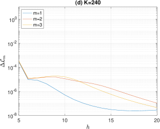
Figure 2: Log-likelihood variations versus the iteration number $h$ of the EM algorithm for different values of $K$.

(a) AIC-based

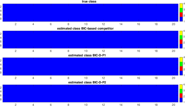
(b) BIC-based

(c) GIC-based

Figure 3: Classification results for a single MC trial under $H_{0}$.

(a) AIC-based

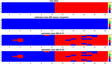
(b) BIC-based

(c) GIC-based

Figure 4: Classification results for a single MC trial under $H_{1,1}$.

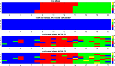
(a) AIC-based

(b) BIC-based

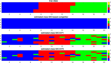
(c) GIC-based

Figure 5: Classification results for a single MC trial under $H_{1,2}$.

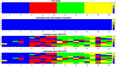
(a) AIC-based

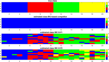
(b) BIC-based

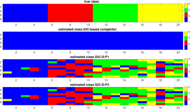
(c) GIC-based

Figure 6: Classification results for a single MC trial under $H_{1,3}$.

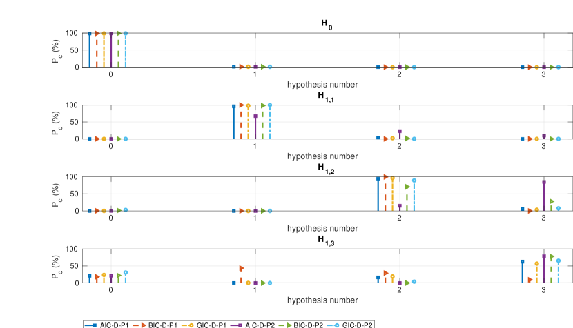
Figure 7: $P_{c}$ ($\%$) versus $H_{0}$ and $H_{1,m}$, $m=1,2,3$, assuming that $K=120$.

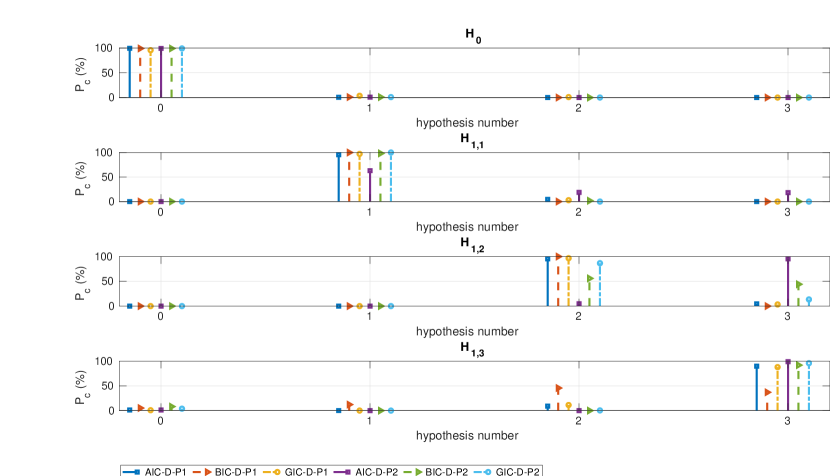
Figure 8: $P_{c}$ ($\%$) versus $H_{0}$ and $H_{1,m}$, $m=1,2,3$, assuming that $K=180$.

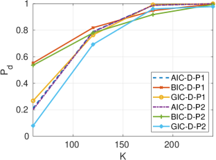
(a) $P_{d}$

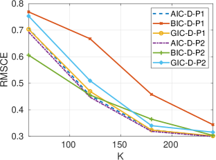
(b) RMSCE

Figure 9: $P_{d}$ and RMSCE versus $K$ assuming that $H_{1,3}$ is true.

IV-A Simulated Data

The simulated data obey the multivariate circular complex Gaussian distribution with zero mean and nominal covariance matrices related to four scenarios: no symmetry, reflection, rotation, and azimuth symmetries. Specifically, they are given by

$${\mbox{\boldmath$C$}}_{1} =\begin{bmatrix}1&0.2+0.3j&0.5-0.3j\\ 0.2-0.3j&0.25&-0.2-0.2j\\ 0.5+0.3j&-0.2+0.2j&0.8\end{bmatrix},$$ (54)

$${\mbox{\boldmath$C$}}_{2} =\begin{bmatrix}1&0&0.5-0.3j\\ 0&0.25&0\\ 0.5+0.3j&0&0.4\end{bmatrix},$$ (55)

$${\mbox{\boldmath$C$}}_{3} =\begin{bmatrix}1&0.3j&0.2\\ -0.3j&0.4&0.3j\\ 0.2&-0.3j&1\end{bmatrix},$$ (56)

$${\mbox{\boldmath$C$}}_{4} =\begin{bmatrix}1&0&0.5\\ 0&0.25&0\\ 0.5&0&1\end{bmatrix},$$ (57)

respectively. In the numerical examples below, the number of data ($K$) ranges from $60$ to $240$, and data are partitioned into adjacent subsets characterized by different PCM structures. The parameter $\rho$ (of GIC-based architectures) is set to $3$ for the competitor [11], $1.3$ for GIC-D-P1, and $11$ for GIC-D-P2 (these values are selected in order to guarantee a good compromise between underestimation and overestimation of the model order). Finally, we consider $P_{fa}=10^{-2}$ and the related detection thresholds are estimated as follows

1. compute the detection threshold under $H_{0}$ and for each PCM structure;

2. the final threshold (namely, $\eta$ in (12)) is set by selecting the maximum of the thresholds obtained at the previous step.

The above procedure guarantees that the actual $P_{fa}$ is less than or equal to the nominal $P_{fa}$.

As a preliminary analysis, we focus on the requirements of the proposed procedures in terms of the EM iterations. To this end, in Figure 2, we plot the log-likelihood variations, i.e., $\Delta\mbox{$\mathcal{L}$}_{m}(h)$, $m=1,2,3$, as a function of $h$, averaged over 1000 MC trials. It turns out that, for all the analyzed cases, a number of 10 iterations (this value will be used in the subsequent analysis) is sufficient to ensure log-likelihood variations less than $10^{-4}$, namely, $\epsilon_{m}<10^{-4}$.

In Figures 3-6, we investigate the instantaneous behavior of the proposed architectures by showing the classification outcomes of a single Monte Carlo trial using a window of size $9\times 20$. These figures are obtained by generating data as follows

• under $H_{0}$, all data share ${\mbox{\boldmath$C$}}_{1}$;

• under $H_{1,1}$, data are split in two equal parts, where the PCM of the first and second halves are ${\mbox{\boldmath$C$}}_{1}$ and ${\mbox{\boldmath$C$}}_{2}$, respectively;

• under $H_{1,2}$, data are partitioned into three subsets with the same cardinality and characterized by ${\mbox{\boldmath$C$}}_{1}$, ${\mbox{\boldmath$C$}}_{2}$, and ${\mbox{\boldmath$C$}}_{3}$;

• under $H_{1,3}$, four equal subsets are generated and, clearly, all the PCMs are used.

In these figures, the estimated structure is mapped to its structure index, namely, $i$ ($\in\{1,\ldots,4\}$) means that ${\mbox{\boldmath$C$}}_{i}$ has been selected. The ground truth is reported at the beginning of each subfigure. From the figures’ inspection, it is evident the advantage (at least from a qualitative point of view) of the proposed architectures over the considered competitor [11], when $H_{1,m},m=1,\dots,3$, is in force. Moreover, as expected, by comparing the four figures, it is possible to observe that $H_{1,3}$ represents the most challenging scenario with the major difficulties in correctly classifying the azimuth symmetry (yellow pixels present in the last partition of data set). As a matter of fact, AIC-D-P1, AIC-D-P2, BIC-D-P2, GIC-D-P1, and GIC-D-P2 are capable of only partially classifying such pixels as characterized by azimuth symmetry.

A more quantitative analysis is performed in Figures 7 and 8 that show the histograms of correct classification over $1000$ independent MC trials assuming $K=120$ and $K=180$, respectively. Such histograms are representative of the probability of correct classification ($P_{c}$) defined as the probability of declaring $H_{0}$ or $H_{1,m}$, $m=1,\dots,3$, under $H_{0}$ or $H_{1,m}$, respectively. As expected, under $H_{0}$, all the proposed architectures return $P_{c}$ values very close to 100$\%$. Under $H_{1,1}$, all the considered architectures can provide percentages of correct classification close to 100$\%$ except for AIC-D-P2 whose $P_{c}$ values are around $0.70$. Almost similar behaviors can be observed under $H_{1,2}$ with the difference that architectures based upon the second EM-based procedure have lower classification capabilities with respect to the results under $H_{1,1}$. Under this hypothesis, the performance of AIC-D-P2 is very poor due to a strong overestimation inclination. Such inclination is also experienced by BIC-D-P2 for $K=180$ since the resulting $P_{c}$ is about $0.56$. Under $H_{1,3}$, which represents the most challenging case, we notice that for $K=120$ the classification values are below $0.75$ for all the considered architectures with BIC-D-P1 returning the worst performance. When $K$ increases to $180$, the situation is clearly better than for $K=120$ even though the classification performance of BIC-D-P1 is less than $0.5$. The other architectures ensure $P_{c}$ values greater than 92$\%$.

The curves reported in Figure 9 pertain to the probability of PCM variation detection ($P_{d}$) and the normalized root mean square classification error (RMSCE) values both as functions of $K$; notice that the $P_{d}$ is defined as the probability of rejecting $H_{0}$ under $H_{1,m}$, whereas the RMSCE is the root mean square number of misclassified vectors divided by $K$. Data are generated under the most challenging hypothesis $H_{1,3}$ and, again, the performance parameters are estimated over $1000$ MC independent trials. From Subfigure 9(a), it turns out that the curves associated with the considered architectures are close to each other when $K>120$ with a maximum difference of about $0.1$. This difference becomes negligible as $K$ increases. As a matter of fact, AIC-D-P1, AIC-D-P2, and GIC-D-P1 are capable of achieving $P_{d}=1$ at $K=240$, whereas BIC-D-P1, BIC-D-P2, and GIC-D-P2 return $P_{d}=0.998$, $P_{d}=0.994$, and $P_{d}=0.978$, respectively, at $K=240$. In Subfigure 9(b), we plot the normalized RMSCE versus $K$. The figure points out that the error curves for AIC-D-P1, AIC-D-P2, and GIC-D-P1 are almost overlapped outperforming the other classifiers at least for $K<240$. The worst performance is returned by BIC-D-P1 as expected from the analysis of the classification histograms.

Summarizing, the above analysis indicates that AIC-D-P1, GIC-D-P1, and AIC-D-P2 can guarantee an excellent compromise between detection performance and classification results under each hypothesis for $K>120$. In addition, notice that if we consider subsets of hypotheses, other architectures can provide reliable classification and detection performance starting from $K=120$.

IV-B Real Recorded Data

In this last subsection, we consider the fully polarimetric SAR data acquired by the EMISAR airborne sensor in the L-band (1.25 GHz). The set is formed by 1750 rows and 1000 columns. The scene under investigation is over the Foulum Area, Denmark, and contains a mixed urban, vegetation, as well as water scene (as shown in Figure 10). Therefore, it is representative of different scattering mechanisms that allow us to suitably verify the classification capabilities of the proposed algorithms in a real-world manifold scenario. The rectangular boxes in the figure highlight the two urban areas of Tjele and Orum.

In Figure 11, the classification maps for all the proposed architectures are shown along with the classification results of the competitor [11]. A window of size $11\times 11$ pixels is used and the threshold is set to the value obtained with the synthetic simulations. The figure clearly sheds light on the fact that the proposed architectures are capable of providing enhanced details and finer resolutions with respect to the competitor due to the inherent best classification capabilities. In all the considered cases, the absence of symmetry (blue pixels) is revealed over the water. Red pixels indicating a detected reflection symmetry, in place of crops and bare fields, are predominant for the BIC- and GIC-like architectures. Yellow pixels (azimuth symmetry) are classified in the presence of forest areas. Rotation symmetries (green pixels) are very few for the classification maps obtained by the competitor, whereas, they are more present in the results obtained with the proposed architectures and appear in the regions containing buildings (for example in the two highlighted urban areas) and roads (that are more clearly visible for the proposed architectures with respect to the competitor).

V Conclusions

In this paper, we have addressed the problem of detecting and classifying PCM structure variations within a data window moving over a polarimetric SAR image. Unlike existing classification procedures that assume a specific PCM structure for all vectors belonging to the sliding window, in this case, data might exhibit different unknown PCM structures. More importantly, the partition of the entire data set according to the respective PCM structures is unknown and must be estimated. This problem naturally leads to a multiple hypothesis test with only one null hypothesis and multiple alternative hypotheses. In order to avoid a significant computational load, we have devised a design framework, grounded on hidden random variables, which assign a PCM label to data vectors, and the EM algorithm tailored to the considered PCM structures.

The performance analysis, conducted on both simulated and real-recorded data also in comparison with a suitable competitor, has highlighted that AIC-D-P1, GIC-D-P1, and AIC-D-P2 are capable of providing an excellent compromise between detection and classification performance under all the considered hypotheses and for $K>120$. In addition, if we restrict the set of hypotheses of interest, other architectures can guarantee good classification/detection performance at least for values of $K$ greater than $120$.

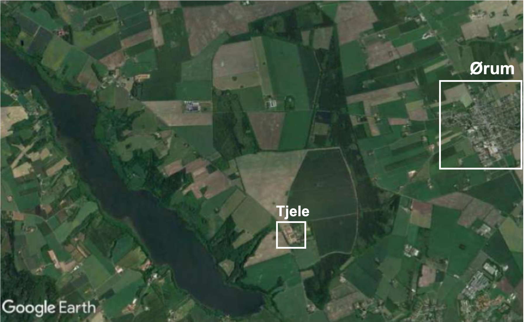
Figure 10: Optical image of the observed scene (drawn from Google Earth ©).

Future research tracks might encompass the extension of such architectures to the heterogeneous environment where the reflectivity coefficient within the window under investigation is not spatially stationary.

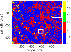
(a) AIC-based competitor

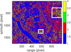
(b) AIC-D-P1

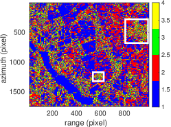
(c) AIC-D-P2

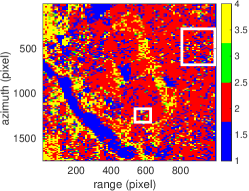
(d) BIC-based competitor

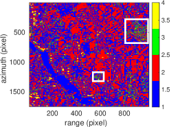
(e) BIC-D-P1

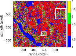
(f) BIC-D-P2

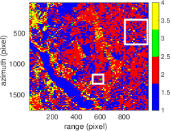
(g) GIC-based competitor

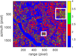
(h) GIC-D-P1

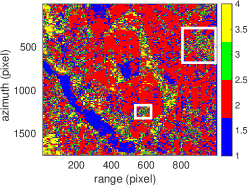
(i) GIC-D-P2

Figure 11: Classification maps with real SAR data: urban area of Tjele (small rectangle) and Orum (great rectangle).

References

• [1] F. Biondi, P. Addabbo, C. Clemente, and D. Orlando, “Measurements of Surface River Doppler Velocities With Along-Track InSAR Using a Single Antenna,” IEEE Journal of Selected Topics in Applied Earth Observations and Remote Sensing, vol. 13, pp. 987–997, 2020.
• [2] F. Biondi, A. Tarpanelli, P. Addabbo, C. Clemente, and D. Orlando, “Water Level measurement using COSMO-SkyMed Synthetic Aperture Radar,” in 2020 IEEE 7th International Workshop on Metrology for AeroSpace (MetroAeroSpace), 2020, pp. 148–153.
• [3] J. Zheng, T. Su, L. Zhang, W. Zhu, and Q. H. Liu, “ISAR Imaging of Targets With Complex Motion Based on the Chirp Rate–Quadratic Chirp Rate Distribution,” IEEE Transactions on Geoscience and Remote Sensing, vol. 52, no. 11, pp. 7276–7289, 2014.
• [4] A. Salberg, O. Rudjord, and A. H. S. Solberg, “Oil Spill Detection in Hybrid-Polarimetric SAR Images,” IEEE Transactions on Geoscience and Remote Sensing, vol. 52, no. 10, pp. 6521–6533, 2014.
• [5] S. Mermoz, S. Allain-Bailhache, M. Bernier, E. Pottier, J. J. Van Der Sanden, and K. Chokmani, “Retrieval of River Ice Thickness From C-Band PolSAR Data,” IEEE Transactions on Geoscience and Remote Sensing, vol. 52, no. 6, pp. 3052–3062, 2014.
• [6] L. M. Novak, S. D. Halversen, G. Owirka, and M. Hiett, “Effects of polarization and resolution on SAR ATR,” IEEE Transactions on Aerospace and Electronic Systems, vol. 33, no. 1, pp. 102–116, 1997.
• [7] D. Gaglione, C. Clemente, L. Pallotta, I. Proudler, A. De Maio, and J. J. Soraghan, “Krogager decomposition and Pseudo-Zernike moments for polarimetric distributed ATR,” in 2014 Sensor Signal Processing for Defence (SSPD), 2014, pp. 1–5.
• [8] F. Garestier, P. Dubois-Fernandez, X. Dupuis, P. Paillou, and I. Hajnsek, “PolInSAR analysis of X-band data over vegetated and urban areas,” IEEE Transactions on Geoscience and Remote Sensing, vol. 44, no. 2, pp. 356–364, 2006.
• [9] A. Lönnqvist, Y. Rauste, M. Molinier, and T. Häme, “Polarimetric SAR Data in Land Cover Mapping in Boreal Zone,” IEEE Transactions on Geoscience and Remote Sensing, vol. 48, no. 10, pp. 3652–3662, 2010.
• [10] S. V. Nghiem, S. H. Yueh, R. Kwok, and F. K. Li, “Symmetry properties in polarimetric remote sensing,” Radio Science, vol. 27, no. 5, pp. 693–711, 1992.
• [11] L. Pallotta, C. Clemente, A. De Maio, and J. J. Soraghan, “Detecting Covariance Symmetries in Polarimetric SAR Images,” IEEE Transactions on Geoscience and Remote Sensing, vol. 55, no. 1, pp. 80–95, 2017.
• [12] L. Pallotta, A. De Maio, and D. Orlando, “A Robust Framework for Covariance Classification in Heterogeneous Polarimetric SAR Images and Its Application to L-Band Data,” IEEE Transactions on Geoscience and Remote Sensing, vol. 57, no. 1, pp. 104–119, 2019.
• [13] A. P. Dempster, N. M. Laird, and D. B. Rubin, “Maximum Likelihood from Incomplete Data via the EM Algorithm,” Journal of the Royal Statistical Society (Series B - Methodological), vol. 39, no. 1, pp. 1–38, 1977.
• [14] P. Addabbo, S. Han, F. Biondi, G. Giunta, and D. Orlando, “Adaptive Radar Detection in the Presence of Multiple Alternative Hypotheses Using Kullback-Leibler Information Criterion-Part I: Detector designs,” IEEE Transactions on Signal Processing, pp. 1–1, 2021.
• [15] P. Stoica and Y. Selen, “Model-order selection: A review of information criterion rules,” IEEE Signal Processing Magazine, vol. 21, no. 4, pp. 36–47, 2004.
• [16] J. Lee and E. Pottier, Polarimetric Radar Imaging: From Basics to Applications, ser. Optical Science and Engineering.   CRC Press, 2017.
• [17] P. Addabbo, S. Han, D. Orlando, and G. Ricci, “Learning Strategies for Radar Clutter Classification,” IEEE Transactions on Signal Processing, vol. 69, pp. 1070–1082, 2021.
• [18] H. Van Trees, Optimum Array Processing: Part IV of Detection, Estimation, and Modulation Theory, ser. Detection, Estimation, and Modulation Theory.   Wiley, 2004.
• [19] K. Murphy, Machine Learning: A Probabilistic Perspective, ser. Adaptive Computation and Machine Learning series.   MIT Press, 2012.
• [20] H. Lütkepohl, Handbook of Matrices, ser. Handbook of Matrices.   Wiley, 1996.