Customizing Graph Neural Networks using Path Reweighting

Abstract

Graph Neural Networks (GNNs) have been extensively used for mining graph-structured data with impressive performance. We argue that the paths in a graph imply different semantics for different downstream tasks. However, traditional GNNs do not distinguish among various downstream tasks. To address this problem and learn the high-level semantics for specific task, we design a novel GNN solution, namely Customized Graph Neural Network with Path Reweighting (CustomGNN for short). CustomGNN can automatically learn the high-level semantics for specific downstream tasks, highlight semantically relevant paths, and filter out task-irrelevant information in the graph. In addition, we analyze the semantics learned by CustomGNN and demonstrate its ability to avoid the three inherent problems in traditional GNNs, i.e., over-smoothing, poor robustness, and overfitting. In experiments with the node classification task, CustomGNN achieves state-of-the-art accuracies on 6 out of 7 datasets and competitive accuracy on the rest one.

1 Introduction

Graph-structured data sets are receiving increasing attentions since they reflect real-world data such as biological networks, social networks, citation networks, and Word Wide Web. In fact, mining graph structure is useful in various real-world problems. Many works focus on semi-supervised learning with graph data [1, 2, 3, 4, 5]; they model the non-Euclidean space of a graph and learn structural information. Among these works, the most notable branch of studies is Graph Neural Networks (GNNs), which embed graph-structured data through feature propagation [3, 6, 7, 8, 9, 10, 11].

Intuitively, on a graph, different applications require different path weighting strategies to emphasize task-related paths and de-emphasize irrelevant ones. For example, if we want to optimize a node classification model by exploiting a paper citation graph, the paths between nodes from intra-class should be emphasized and the paths between nodes from inter-class should be de-emphasized. Concretely, given a citation graph, where path weight captures the relevance among categories. If the downstream task is node classification, the paths with more nodes in the same category will be emphasized more. If the downstream task is to find papers in a specific category (e.g., AI category), then a path contains more nodes relevant to this category (AI) will be selected.

However, traditional GNNs have ignored the differences among paths, which also leads to some potential problems. Gilmer et al. [12] states that GNNs can be regarded as a message-passing method with a low-passing filter, resulting in exponentially information lost with the increment of propagation steps, i.e., the problem of over-smoothing [13, 14, 15]. Although some current GNN SOTAs, such as GRAND [16], GraphMix [17] and S²GNN [18], have considered multi-hop information, they are still based on the theory of message-passing on a graph and ignore the differences among different paths, which also leads to the injection of task irrelated information and the loss of important information in the message-passing process. It seems hard to differentiate different paths with various hops by the message-passing method. But if we look at it in another light, if we could extract the high-level semantics of different paths, and aggregate the high-order information directly instead of passing messages hop by hop, we can avoid the loss of information and injection of noises while differentiating different paths. On the other hand, the poor robustness to graph attack [19, 20] of traditional GNNs also comes from they cannot filter out irrelevant paths and noises. Essentially, the propagation step aggregates all neighborhoods’ information with noises, while some noisy nodes and edges may dominate the representation learning procedure. The third issue derived from semi-supervised learning is that, traditional training processes for GNNs can easily overfit the lacking labeled data [21].

By considering these intuitions, we propose Customized Graph Neural Network with Path Reweighting (CustomGNN). CustomGNN differentiates paths by extracting their high-level semantics and customizes node (graph) embeddings for specific downstream tasks by aggregating high-order information directly. In detail, customGNN first generates multi-perspective subgraphs; then, it calculates multiple path attention maps by extracting specific high-level semantic information from these subgraphs through a neural network with LSTM-based path weighting strategy; after that, customGNN aggregates features through these path attention maps; at last, it infuses these features with a multi-hop GNN. As a consequence, CustomGNN can automatically filter out noises and encode the most useful structural information for a specific task.

Finally, we analyze the semantics of path weights for node classification task. We also empirically demonstrate that our method can effectively avoid the issues of over-smoothing and non-robustness, while mitigating the issue of overfitting. Moreover, we show the novel components proposed in this paper bring significant improvement in ablation experiments.

Our contributions can be concluded as follows:

• We propose a novel GNN architecture, named CustomGNN (Customized Graph Neural Network with Path Reweighting), which extracts task-oriented semantic features from re-weighted paths in sub-graphs and infuses the extracted information with a standard multi-hop GNN. With this design, CustomGNN can automatically filter out noises and encode the most useful path structural information for a specific task.

• We propose two unsupervised loss functions to regularize the learning procedure of CustomGNN. First, we use random walk to generate multi-perspective sub-graphs and apply consistency loss in-between. Second, to enhance the semantics, we use unlabeled data to generate pseudo-labels, and apply triplet loss based on these pseudo-labels. To our knowledge, this is the first work to adopt triplet loss with pseudo-labels in GNNs.

• As demonstrated by comprehensive experiments and analyses, the proposed CustomGNN model achieves state-of-the-art results on seven widely-used graph node classification datasets. It shows good interpretability and effectively mitigates the issues of over-smoothing, non-robustness and overfitting.

2 Related Work

2.1 Graph Neural Networks

Graph neural networks (GNNs) [1, 6, 11, 22] aim to learn the graph-structured information. They learn a vector representation for each node by aggregating its neighbors’ information. The core difference among different GNNs is the message passing (aggregation) method [12]. For example, to aggregate information, GCN [3] proposes graph convolution layer, and GAT [8] presents graph attention layer. Recently, lots of works focus on resolving the issue of over-smoothing for deep GNNs [10, 9, 18, 23]. CustomGNN provides a novel view to learn the graph-structured data, which focuses on learning the high-level semantics of paths for specific downstream applications. This method can naturally prevent the above-mentioned issues of traditional GNNs.

2.2 Graph Representation Learning

Given a graph, node representation aims to learn the low dimensional vector representation of each node and its graph-structured information. There have emerged many methods for node embedding in recent years. These methods can mainly be divided into two categories according to the input graph. The first is sampling based methods which uses random walk [2, 24, 25] or other sampling strategies to sample subgraphs as the input data [7, 26]. The advantage of these methods is that they learn the local information of a graph, which can improve the model’s generalization and reduce space consumption. The second is inputting the whole graph [3, 8], and conducing graph neural network on it to learn the node attributes and graph structure jointly. In addition, some advanced methods have been emerged recently, for example, Xu et al. [5] disentangle the single representation of node attributes and graph structure into two different representations respectively. In this paper, we leverage the advantages of sampling based method to learn the customized high-level semantic information, as well as the advantages of traditional GNNs to learn the generic graph information.

2.3 Semi-Supervised Learning on Graph

One research direction for semi-supervised learning on graphs is to assign pseudo-labels to unlabeled data. Here, in order to utilize the unlabeled data, Lee [27] first used neural network to infer pseudo-labels of unlabeled data. Elezi et al. [28], Iscen et al. [29] used label propagation for pseudo-labels in the field of computer vision. Yang et al. [30] and Hao et al. [31] performed the label propagation and pseudo-labels in the field of GNN. Schroff et al. [32] used triplet loss to enhance the uniqueness of different faces for face recognition. Similarly, for semi-supervised learning, CustomGNN combined the pseudo-labels with triplet loss to enhance the semantics of each path.

A second research direction for semi-supervised learning on graphs is to design powerful regularization methods for regularizing graph neural networks [33, 16, 17, 34, 35, 36]. For example, VBAT [34] and GraphVAT [35] adopted consistency loss in GNNs by virtual adversarial training; GraphMix [17] introduced the mixup strategy [37] in GNNs by utilizing linear interpolation between two nodes for data augmentation; and GRAND [16] used the DropNode method (which is similar to DropEdge [33]) to perturb the graph structure for data augmentation. In contrast, we perform random walks to generate various sub-graphs in each iteration. Each of these sub-graphs could represent a distinct view of the whole graph. After multiple iterations, we get multi-perspective sub-graphs and we compute the consistency loss among them for regularization.

3 The Proposed Method

The overall architecture of CustomGNN is illustrated in Figure 1. Given a graph $G$ with encoded features, we develop a path re-weighting module (blue stream) to capture the customized high-level semantic information, and a multi-hop GNN module (orange stream) to capture the generic graph information. The most salient part proposed in CustomGNN is to re-weight each sub-path by an LSTM-based neural network model, which customizes the paths’ importance for a specific downstream task. Table 1 provides the definitions of the notations we used in this paper.

Notation	Definition
$\mathbf{A}$	The input adjacent matrix of the given graph $G$.
$\mathbf{F}$	The input features.
$\widetilde{\mathbf{F}}$	The output features of feature encoder (Section 3.1).
$\hat{\mathbf{F}}$	The aggregated features after semantic aggregation (Section 3.3).
$\dot{\mathbf{F}}$	The output features of multi-hop gnn module.
$\overline{\mathbf{F}}$	The final concatenated embeddings ($\{\overline{\mathbf{F}}|\mathbf{F}=\hat{\mathbf{F}}\oplus\dot{\mathbf{F}}\}$).
$\mathbf{P^{(k)}_{ij}}$	$k^{th}$ path between node $i$ and node $j$, each row is drawn from $\widetilde{\mathbf{F}}$.
$\mathbf{W}$	The weight matrix computed by LSTM (Section 3.2.2).
$\mathbf{Z}$	The final predictions of classifier.
$\mathbf{\theta_{1}}$	The trainable parameters of encoder.
$\mathbf{\theta_{2}}$	The trainable parameters of LSTM.
$\mathbf{\theta_{3}}$	The trainable parameters of classifier (MLP).
$\mathcal{L}_{sup}$	The supervised loss computed from Eq (6).
$\mathcal{L}_{unsup}$	The unsupervised loss consisted of $\mathcal{L}_{con}$ and $\mathcal{L}_{tri}$ (Eq (5)).
$\mathcal{L}_{con}$	The consistency loss computed from Eq (7).
$\mathcal{L}_{tri}$	The triplet loss computed from Eq (9).

Table 1: The definitions of notations.

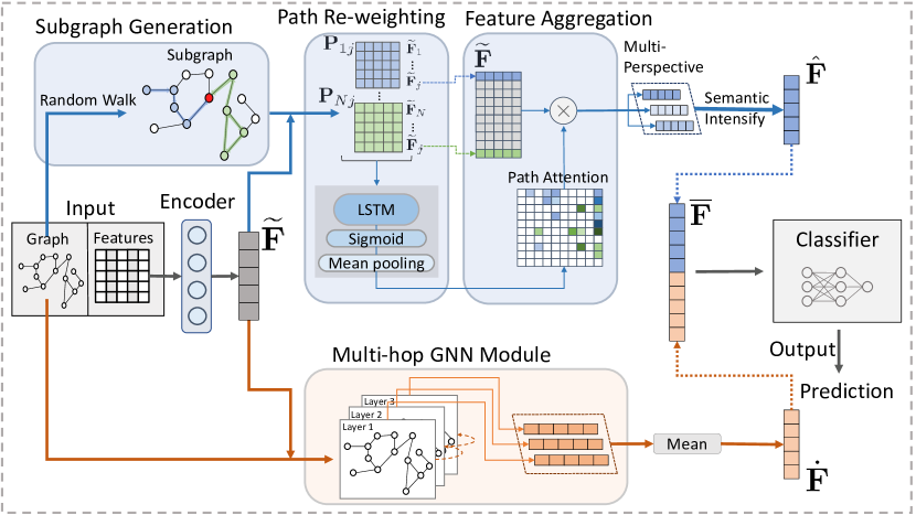
Figure 1: The overall architectural diagram of CustomGNN. There are two paths in CustomGNN. The first path highlighted in blue uses random walk to generate sub-paths (a sub-graph), then, the path re-weighting module is utilized in these sub-paths for generating customized feature $\hat{\mathbf{F}}$; The orange line indicates that we use simple multi-hop GNN to generate general feature $\dot{\mathbf{F}}$. Finally, we feed the aggregated feature $\{\overline{\mathbf{F}}|\mathbf{F}=\hat{\mathbf{F}}\oplus\dot{\mathbf{F}}\}$ into classifier to obtain the predictions.

3.1 Feature Encoder

Let $n$ and $d$ represent the number of nodes and the feature dimension respectively. In the beginning, a feature encoder $f_{enc}$ is employed to compress the sparse features $\mathbf{F}\in\mathbb{R}^{n\times d}$ into low dimensional dense features $\{\widetilde{\mathbf{F}}=f_{enc}(\mathbf{F};\mathbf{\theta}_{1})|\widetilde{\mathbf{F}}\in\mathbb{R}^{n\times D}\}$, where $D$ denotes the dimension of encoded features. The encoder $f_{enc}(\cdot)$ can be written as follow, $f_{enc}(\mathbf{F};\mathbf{\theta}_{1})=\mathbf{F}\cdot\mathbf{\theta}_{1}$, where $\mathbf{\theta}_{1}\in\mathbb{R}^{d\times D}$ are the trainable parameters for the encoding layer.

3.2 LSTM-based Path Re-weighting

3.2.1 Sub-graph Generation

A random walk on the graph could generate multiple paths and extract corresponding node pairs. For example, setting the window size to 3 and path length to 4, we can get a path $(x_{1},x_{2},x_{3},x_{4})$ and a set of sub-paths, i.e., $(x_{1},x_{2})$, $(x_{2},x_{3})$, $(x_{3},x_{4})$, $(x_{1},x_{2},x_{3})$, $(x_{2},x_{3},x_{4})$. The starting and ending node in each sub-path construct a node pair. As illustrated in Figure 1, we perform multiple random walks from a single point, which will generate multiple paths with the same starting node. These paths with the same starting point can be regarded as a sub-graph. Therefore, a sub-graph can be generated by multiple random walks.

3.2.2 Path Re-weighting

In traditional GNNs such as GCN [3], GCNII [10], SGC [9] and S²GC [18], paths were equally treated in their loss functions. Some other methods, such as GAT [8], have computed the attention between a node pair, however, this attention is computed mainly according to the similarity of the node features, and the specific high-level semantic information (such as the importance of paths between this pair of nodes) has been lost. Therefore, attention learned in this way is not always optimal for a given downstream task. To better understand the importance of path re-weighting, we take the Wikipedia knowledge graph as an example. Each path in the graph reflects a piece of knowledge in a particular domain. If we want to enhance the performance of medical Q&A by exploiting Wikipedia knowledge graph, some general knowledge that is not related to the medical domain should be de-emphasized. Thus, we re-weight the paths to indicate their importance scores so that the essential knowledge for a specific task can be selected.

In the path re-weighting step, we generate path weight $w_{ij}$ for a node pair $(x_{i},x_{j})$. On account of homophily assumption [38], nodes with the same label are more likely to be appeared in a same sub-graph, so a sub-graph must imply some semantic information about the labels. Therefore, the challenge is how to extract the implicit high-level semantics from sub-graphs (paths). Naturally, we can use a sequence model (e.g., LSTM [39]) to extract the high-level semantic information from paths.

Formally, if we have a node pair $(x_{i},x_{j})$ and paths (from $x_{i}$ to $x_{j}$) $\mathbf{P}_{ij}^{(0)}$, … , $\mathbf{P}_{ij}^{(k)}$, … , $\mathbf{P}_{ij}^{(N-1)}$, the path weight $w_{ij}$ can be computed by the followed formulation:

$$\small w_{ij}=\frac{1}{N}\sum_{k=0}^{N-1}S(f_{lstm}(\mathbf{P}_{ij}^{(k)};\mathbf{\theta}_{2})),$$ (1)

where $f_{lstm}$ and $\theta_{2}$ denote the LSTM model and the trainable parameters of LSTM respectively. The path matrix $\mathbf{P}_{ij}\in\mathbb{R}^{L\times D\times N}$ is the feature representation of sampled path sequences, where $L$, $D$ and $N$ represent the path length, dimension of $\widetilde{\mathbf{F}}$ and the number of paths between the node pair $(x_{i},x_{j})$.

3.3 Semantic Aggregation

3.3.1 Re-weighted Attention

We aggregate the semantic information from re-weighted paths in an attention matrix. Concretely, the path weights $\{w_{ij}|0\leq i,j<n\}$ are used to construct path attention matrix $\mathbf{W}\in\mathbb{R}^{n\times n}$ whose role is similar to the attention matrix in GAT or the Laplacian matrix in GCN. Each weight value $w_{ij}$ is an entry of $\mathbf{W}$.

3.3.2 Feature Aggregation

In this step, we conduct a convolution operation on $\mathbf{W}$ to embed features $\widetilde{\mathbf{F}}$. This operation could aggregate the high-level semantic information of a sub-graph to center node ($j^{th}$ node) of this sub-graph. The aggregating operation can be expressed as follow:

$$\small\hat{\mathbf{F}}_{j}=\sum_{i=0}^{n-1}w_{ij}\cdot\widetilde{\mathbf{F}}_{ij},$$ (2)

where $w_{ij}$ is the attention (weight) value of $i^{th}$ node to $j^{th}$ node, $n$ represents the number of nodes, and $\hat{\mathbf{F}}_{j}$ denotes the node embedding of $j^{th}$ node.

3.4 Infusion with Multi-hop GNN

3.4.1 Multi-hop GNN

To prevent some graph-structured information from being lost, the multi-hop GNN module is used to learn the generic graph information. In this module, we compute the means of all graph convolutional layers’ output $\dot{\mathbf{F}}$. Formally, $\dot{\mathbf{F}}$ is computed as follow:

$$\small\dot{\mathbf{F}}=\frac{1}{H+1}\sum^{H}_{h=0}\mathbf{A}^{h}\cdot\widetilde{\mathbf{F}},$$ (3)

where $H$ is a hyperparameter which denotes the number of graph convolutional layers.

3.4.2 Semantic Infusion

Finally, we infuse the high-level semantic information into generic graph information by concatenating $\hat{\mathbf{F}}$ and $\dot{\mathbf{F}}$, and feed them into a MLP followed by a softmax function $\sigma(\cdot)$ to get the prediction $Z$. The equation can be written as $\mathbf{Z}=\sigma(f_{mlp}(\dot{\mathbf{F}}\oplus\hat{\mathbf{F}}|\theta_{3}))$, where $\theta_{3}$ is the trainable parameters of MLP, and $\oplus$ represents the concatenating operation.

3.5 Loss Function and Joint Training

In semi-supervised learning problem, most training data are unlabeled, so, how to leverage these unlabeled data is important. Firstly, in the sub-graph generation process (Section 3.2.1), we randomly sample some sub-graphs each iteration, these sub-graphs can be seen as a new perspective of our data. Then, we use consistency regularization in these perspectives. Secondly, we want to enhance the distinctiveness of path semantics. In doing so, we first using path re-weighting module to extract the semantic of each paths, and then, we minimize the distance of same semantic and maximize the distance of different one via triplet loss function. The unsupervised loss consist of the two parts. The whole training and predicting process is stated in Algorithm 1. Next, we will introduce our training process detailedly.

3.5.1 Overall Loss Functions

As formulated in Eq (4), our loss function contains supervised and unsupervised loss, and we use $\lambda$ to control the trade-off between them:

$$\mathcal{L}=\mathcal{L}_{sup}+\lambda\mathcal{L}_{unsup}.$$ (4)

The unsupervised loss is a combination of the triplet loss (Eq (9)) and consistency loss (Eq (7)) showed in Eq (5), and we use two hyper-parameters $\lambda_{1}$ and $\lambda_{2}$ to control the balance of the two parts:

$$\small\mathcal{L}_{unsup}=\lambda_{1}\mathcal{L}_{con}+\lambda_{2}\mathcal{L}_{tri}.$$ (5)

With labeled data $\mathbf{Y}^{L}$ and the predictions $\mathbf{Z}^{(s),L}$ from MLP, we compute the average entropy loss of $\{\mathbf{Z}^{(s),L}|1\leq s\leq S\}$:

$$\small\mathcal{L}_{sup}=-\frac{1}{S}\sum^{S}_{s=1}[\mathbf{Y}^{L}\log{\mathbf{Z}^{(s),L}}+(1-\mathbf{Y}^{L})\log{(1-\mathbf{Z}^{(s),L})}].$$ (6)

Algorithm 1 CustomGNN

Input: adjacency matrix $\mathbf{A}$, feature matrix $\mathbf{F}$, training labels $\mathbf{Y}^{L}$;
Hyperparameters: loss tradeoff parameter $\lambda$, learning rate $\eta$, GNN propagation step $H$, times for regularization in each epoch $S$;
Parameters: encoder $f_{enc}(\mathbf{F};\theta_{1})$, sequence model (LSTM) $f_{lstm}(\mathbf{P};\theta_{2})$, classifier $f_{mlp}(\overline{\mathbf{F}};\theta_{3})$.
Output: predictions $\mathbf{Z}$.

1:  while not converged do

2:     initialize $\mathbf{W}$ with $0$;

3:     for s=0 to s <S do

4:        Encode input features as Section 3.1;

5:        Generate sub-graphs for perspective $s$ by random walk;

6:        Construct path attention matrix from sampled paths via Eq (1);

7:        Aggregate sub-graph information via Eq (2);

8:        Semantic enhancing via Eq (9);

9:        Aggregate general graph information via Eq (3);

10:        Semantic infusion and prediction as described in Section 3.4.2: $\mathbf{Z}^{(s)}=\sigma(f_{mlp}(\dot{\mathbf{F}}\oplus\hat{\mathbf{F}}^{(s)}|\theta_{3}))$;

11:     end for

12:     Compute the unsupervised loss $\mathcal{L}_{unsup}$ via Eq (5);

13:     Compute the supervised loss $\mathcal{L}_{sup}$ via Eq (6);

14:     Update the parameters $\theta_{1}$, $\theta_{2}$ and $\theta_{3}$ by gradients descending: $\Theta=\Theta-\eta\nabla_{\Theta}(\mathcal{L}_{sup}+\lambda\mathcal{L}_{unsup})$;

15:  end while

16:  Output prediction $\mathbf{Z}$ as described in Section 3.5.4: $\mathbf{Z}=\sigma(f_{mlp}(\dot{\mathbf{F}}\oplus\hat{\mathbf{F}}))$.

3.5.2 Multi-Perspective Regularization

To improve robustness and prevent over-fitting, we employ consistency regularization [40] in our model to encourage that different perspectives could get a consistent result.

In doing so, we generate $S$ perspectives each epoch, each perspective is constructed by a separate path generation and re-weighting module (Section 3.2), and produce $S$ different feature matrices $\{\hat{\mathbf{F}}^{(s)}|1\leq s\leq S\}$. We concatenate $\hat{\mathbf{F}}^{(s)}$ with multi-hop GNN feature $\dot{\mathbf{F}}$ to get enhanced feature $\{\overline{\mathbf{F}}^{(s)}|\overline{\mathbf{F}}^{(s)}=\dot{\mathbf{F}}\oplus\hat{\mathbf{F}}^{(s)}\}$, the enhanced features $\overline{\mathbf{F}}^{(s)}$ are fed into MLP module to get the predictions $\{\mathbf{Z}^{(s)}|\mathbf{Z}^{(s)}=f_{mlp}(\overline{\mathbf{F}}^{(s)})\}$. The $S$ predictions $\{\mathbf{Z}^{(s)}|1\leq s\leq S\}$ produced from $S$ perspectives are used for consistency regularization.

The purpose of this regularization is to minimize the $L_{2}$ distance among the predictions $\mathbf{Z}^{(s)}$. For example, setting $S=2$, we want to get $min{\left\|\mathbf{Z}^{(1)}-\mathbf{Z}^{(2)}\right\|}^{2}_{2}$. First, we need to get the average prediction for $i^{th}$ node, i.e., $\overline{\mathbf{Z}}_{i}=\frac{1}{S}\sum_{s=1}^{s=S}\mathbf{Z}^{(s)}_{i}$. Then, we sharpen [40] the $\overline{\mathbf{Z}}_{i}$ with temperature $T$, i.e., $\overline{\mathbf{Z}}_{ic}^{\prime}=\overline{\mathbf{Z}}_{ic}^{\frac{1}{T}}/\sum_{c=0}^{C-1}{\overline{\mathbf{Z}}_{ic}^{\frac{1}{T}}}$, where $\overline{\mathbf{Z}}_{ic}^{\prime}$ is the sharpened average prediction of $i^{th}$ node in $c^{th}$ class. Finally, we compute the $L_{2}$ norm distance between the sharpened average prediction and $S$ individual predictions. The consistency loss can be written as:

$$\small\mathcal{L}_{con}=\frac{1}{S}\sum\limits_{s=1}^{S}\sum\limits_{i=0}^{n-1}{\left\|\mathbf{Z}_{i}^{(s)}-\overline{\mathbf{Z}}_{i}^{\prime}\right\|}^{2}_{2}.$$ (7)

3.5.3 Semantic Enhancing with Triplet Loss

Intuitively, the high-level semantics is implied in the labels for node classification task. Therefore, the essence of semantic enhancing is to make the high-level semantic of paths in same label become close and different labels become distant.

$$\small\mathbf{I}_{ij}=\left\{\begin{array}[]{lr}1,&\mathbf{Y}_{i}=\mathbf{Y}_{j}\\ 0,&\mathbf{Y}_{i}\neq\mathbf{Y}_{j}\end{array}\right.$$ (8)

In doing so, we use matrix $\mathbf{I}\in\{0,1\}^{n\times n}$ to denote the label is same or not. In Eq (8), $\mathbf{Y}\in\{0,1\}^{n\times C}$ denotes the one-hot label vector, $C$ represents the number of classes. Notably, the labeled $i^{th}$ node $\mathbf{Y}_{i}\in\mathbf{Y}^{L}$ is from training set directly, the unlabeled $j^{th}$ node $\mathbf{Y}_{j}\in\mathbf{Y}^{U}$ is “guessed” by our model, the pseudo labels can be generated by $\{\mathbf{Y}_{j}=argmax(\mathbf{Z}_{j})|\mathbf{Y}_{j}\in\mathbf{Y}^{U}\}$, where $\mathbf{Z}$ denotes the probabilities predicted by CustomGNN. Then, the positive node pairs $(\hat{\mathbf{F}}_{i}^{pos},\hat{\mathbf{F}}_{j}^{pos})$ and negative node pairs $(\hat{\mathbf{F}}_{i}^{neg},\hat{\mathbf{F}}_{j}^{neg})$ can be sampled out. We use triplet loss [32] to minimize the $L_{2}$ norm distance between positive node pairs and maximize the distance between negative node pairs. The loss function is as follows:

$$\small\mathcal{L}_{tri}={\left\|\hat{\mathbf{F}}_{i}^{pos}-\hat{\mathbf{F}}_{j}^{pos}\right\|}_{2}+RELU(m-{\left\|\hat{\mathbf{F}}_{i}^{neg}-\hat{\mathbf{F}}_{j}^{neg}\right\|}_{2}),$$ (9)

where $m$ is a hyperparameter that represents the margin between negative node pairs.

3.5.4 Inference

To avoid the path attention matrix $W$ being too sparse we compute this matrix $S$ times ($S=4$ in our setting) by $S$ perspectives and add them together to get a new path attention matrix $\{\mathbf{W}|\mathbf{W}=\sum_{s=1}^{S}\mathbf{W}^{(s)}\}$. The final path attention matrix is used to compute $\hat{\mathbf{F}}$ as Eq (2). Meanwhile, $\dot{\mathbf{F}}$ is computed by multi-hop GNN module. At last, the concatenated embedding $\overline{\mathbf{F}}$ is fed into classifier MLP to get the final prediction $\mathbf{Z}$.

4 Experiments

4.1 Datasets

Following the community convention, we use three benchmark graphs, i.e., Cora, Citeseer and PubMed with their standard public splits in Planetoid [2], which contains 20 nodes per class for training and 1000 nodes for testing. We also did experiments on 4 publicly available large datasets, i.e., Cora Full, Coauthor CS, Amazon Photo and Amazon Computers with their experimental settings in Shchur et al. [41].

These datasets can be downloaded from PyTorch-Geometric library. The datasets details are shown in Table 2. Label rate is the fraction of nodes in training set (the number of training nodes are 20 per class) that can be computed as (#class $\cdot$ 20)/#node.

Dataset	Nodes	Edges	Classes	Features	Label Rate
Cora	2708	5429	7	1433	0.0516
Citeseer	3327	4732	6	3703	0.0360
PubMed	19717	44338	3	500	0.0030
Cora-Full	19749	63262	68	8710	0.0689
Coauthor CS	18333	81894	15	6805	0.0164
Amazon Computer	13752	245861	10	767	0.0145
Amazon Photo	7650	119081	8	745	0.0209

Table 2: Details of datasets after preprocessing.

4.2 Baseline

For the 3 standard split datasets, we choose 19 GNN SOTAs for comparison, including GCN [3] and its evolutions [9, 18, 10], deep GNNs like MixHop [37] and APPNP [42], and some other important specific methods. For the other 4 large datasets, we choose baseline methods that can be scaled to large graphs, including a two-layer MLP (input layer $\rightarrow$ hidden layer $\rightarrow$ output layer) with 128-hidden units, standard GCN and GAT, and two regularization based methods, i.e., GRAND [16] (using MLP as the backbone) and P-reg [30] (using GCN as the backbone).

4.3 Overall Results

Method	Cora	Citeseer	PubMed
GCN (2017)	81.5$\pm$ *	70.3$\pm$ *	79.0$\pm$ *
GraphSAGE (2017)	78.9$\pm$0.8	67.4$\pm$0.7	77.8$\pm$0.6
FastGCN (2018)	81.4$\pm$0.5	68.8$\pm$0.9	77.6$\pm$0.5
GAT (2018)	83.0$\pm$0.7	72.5$\pm$0.7	79.0$\pm$0.3
MixHop (2018)	81.9$\pm$0.4	71.4$\pm$0.8	80.8$\pm$0.6
VBAT (2019)	83.6$\pm$0.5	74.0$\pm$0.6	79.9$\pm$0.4
G3NN (2019)	82.5$\pm$0.2	74.4$\pm$0.3	77.9$\pm$0.4
APPNP (2019)	83.8$\pm$0.3	71.6$\pm$0.5	79.7$\pm$0.3
GraphMix (2019)	83.9$\pm$0.6	74.5$\pm$0.6	81.0$\pm$0.6
DropEdge (2020)	82.8$\pm$ *	72.3$\pm$ *	79.6$\pm$ *
Graph U-Net (2019)	84.4$\pm$0.6	73.2$\pm$0.5	79.6$\pm$0.2
SGC (2019)	81.0$\pm$0.0	71.9$\pm$0.1	78.0$\pm$0.0
GMNN (2019)	83.7$\pm$ *	72.9$\pm$ *	81.8$\pm$ *
GraphNAS (2019)	84.2$\pm$1.0	73.1$\pm$0.9	79.6$\pm$0.4
GCNII (2020)	85.5$\pm$0.5	73.4$\pm$0.6	80.2$\pm$0.4
P-reg (2020)	82.8$\pm$1.2	71.6$\pm$2.2	77.37$\pm$1.5
superGAT (2021)	84.3$\pm$0.6	72.6$\pm$0.8	81.7$\pm$0.5
S2GC (2021)	83.5$\pm$0.02	73.6$\pm$0.09	80.2$\pm$0.02
GraphSAD (2021)	83$\pm$0.42	71.23$\pm$0.22	79.56$\pm$0.11
CustomGNN	85.3$\pm$0.6	76.2$\pm$0.4	82.1$\pm$0.3

Table 3: Results on 3 standard split datasets with over 100 runs. Some papers do not report their std values, which are marked by “*”. Bold denotes the best performance, underline denotes the second best.

Method	Cora-Full	Coauthor CS	Amazon Computer	Amazon Photo
MLP	18.3$\pm$4.9	88.3$\pm$0.7	57.8$\pm$7.0	73.5$\pm$9.7
GCN (2017)	9.0$\pm$4.9	88.1$\pm$2.7	42.3$\pm$16.0	61.4$\pm$12.3
GAT (2018)	13.7$\pm$5.2	90.3$\pm$1.4	65.4$\pm$15.3	80.8$\pm$9.5
GRAND (2020)	42.3$\pm$6.5	92.9$\pm$0.5	80.1$\pm$7.2	72.9$\pm$2.1
P-reg (2020)	–	92.6$\pm$0.3	81.7$\pm$1.4	91.2$\pm$0.8
CustomGNN	44.2$\pm$1.2	93.4$\pm$0.3	81.9$\pm$0.8	92.0$\pm$3.4

Table 4: Results on 4 large datasets with over 100 runs on different random seed for train/test set split and different random seed for weight initialization. Bold denotes the best performance, underline denotes the second best and ”–” denotes the original authors does not run this experiment.

Table 3 compares the accuracy of CustomGNN with 19 state-of-the-art methods. The results of these methods are taken from their original papers directly. It shows that CustomGNN gets the competitive result (0.1%) with SOTA on Cora, and achieves the state-of-the-art accuracy on Citeseer and PubMed. It is notable that CustomGNN gets a good improvements on Citeseer, this may because that the citation graph on Citeseer implies more semantics. We will analyze this in Section 4.5.

Table 4 compares the accuracy of CustomGNN with 3 traditional baselines and 2 regularization based GNNs. The experiments strictly follow the evaluation protocol of Shchur et al. [41]. The results of two-layer MLP (input layer $\rightarrow$ hidden layer $\rightarrow$ output layer) with 128-hidden units, GCN, GAT GRAND and CustomGNN are averaged over 100 runs on different random seed for train/test set split and different random seed for weight initialization. The results of P-reg are taken from its original paper. It shows that CustomGNN outperforms the other 5 methods on all 4 large datasets.

4.4 Ablation Study

Table 5 illustrates the results of ablation study. This study evaluates the contributions of different components in CustomGNN.

Component	Cora	Citeseer	PubMed
w\o path re-weighting	79.2(-6.1)	68.7(-7.5)	77.8(-4.3)
w\o multi-hop gnn	83.4(-0.9)	75.4(-0.8)	81.6(-0.5)
w\o triplet loss	84.6(-0.9)	75.2(-1.0)	81.6(-0.5)
w\o multi-perspective	84.2(-1.1)	75.3(-0.9)	79.2(-2.9)
original	85.3	76.2	82.1

Table 5: Ablation studies, the accuracy of CustomGNN without specific component. The number in parentheses is the decay of accuracy after remove this component.

4.4.1 Without Path Re-weighting

We only use the multi-hop GNN module to generate node embeddings, i.e., $\overline{\mathbf{F}}=\dot{\mathbf{F}}$, the path re-weighting module containing unsupervised loss (Eq (5)) is removed. This result can be regarded as a baseline.

4.4.2 Without Multi-hop GNN

We only use the path re-weighting module to generate the final node embeddings, i.e., $\overline{\mathbf{F}}=\hat{\mathbf{F}}$. In addition, to get a dense path attention matrix ($\mathbf{W}$), we sample paths for all nodes, i.e., fixing sampling batch size to #nodes/S.

4.4.3 Without Semantic Enhancing

The unsupervised loss is only computed by consistency regularization loss to show the efficacy of the proposed semantic enhancing method with triplet loss.

4.4.4 Without Multi-Perspective Regularization

The unsupervised loss is only computed by triplet loss to show the efficacy of the proposed multi-perspective regularization method. To this end, we first set $S=1$ for using only one perspective. Second, we sample paths for all nodes to ensure that this perspective can get more complete information. Third, because that there is no consistency regularization, we decrease the dropout rate.

4.5 Analysis

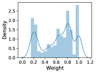
(a) Distribution of re-weighted path attentions.

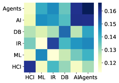
(b) Visualization of relevance between different categories.

Figure 2: (a) The visualization of re-weighted path attentions on Citeseer. We filter out some noisy points whose weight is less than 0.15. (b) The visualization of relevance between different categories on Citeseer. The weight on $(i,j)$ means how much the $i^{th}$ category influenced by $j^{th}$ category.

The re-weighted attentions learned by CustomGNN are customized for different downstream tasks. For example, Figure 2(a) shows the distribution of re-weighted attentions for Citeceer node classification task, which is quite diverse. To better understand these attentions and how CustomGNN benefits the results, we provide some semantic analyses. After that, we study three metrics of our performance, i.e., generalization, robustness, and over-smoothing. In our experiments, we compared CustomGNN with two traditional GNNs (GCN [3] and GAT [8]) and a GNN SOTA (GRAND [16]) which also concentrates on resolving the three issues.

4.5.1 Semantics Explanation

Category	Number
Agents	239
Artificial Intelligence (AI)	537
Data Base (DB)	619
Information Retrieval (IR)	633
Machine Learning (ML)	560
Human–Computer Interaction (HCI)	463

Table 6: Summary of paper citation graph on Citeseer.

In order to mine the semantics of re-weighted paths, we use Citeseer as an example. Papers on Citeseer are classified into 6 categories as described in Table 6. Based on this dataset, the task is to classify a giving paper to its category. After training the model, we generate multiple paths for a pair of nodes, the average of these paths’ weights is the average relevance weight between the corresponding categories of this pair of nodes. We visualize the relevance weights among different categories in Figure 2(b).

Figure 2(b) implies a lot of information. Consistent with our intuition, the average weights of self-loop (computed from paths where the starting and ending nodes are from the same category) is the largest, e.g., weight of (IR,IR) is larger than (IR, others). Moreover, from Figure 2(b), we can see that AI and Agents are highly relevant with each other; AI is much influenced by ML, whereas ML is less influenced by AI; DB influences others more than it is influenced by others, as the column of DB has smaller average weights than its corresponding line in the visualized matrix. All these results coincide with human intuitions.

4.5.2 Weight Correlation

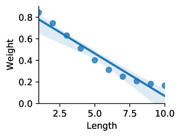
(a) Weight-Length.

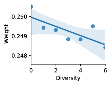
(b) Weight-Diversity.

Figure 3: (a) and (b) are the mean correlations between weight and two properties (length and diversity) of paths on Cora. In (b), to remove the influence of length, the path length is fixed on 10. Y-axis denotes the average weight of the corresponding paths.

To analyze how the properties of paths influence weight scores, we draw the correlations between weight scores and two properties of paths, i.e., length and diversity, on Figure 3. Length is defined as the number of nodes in a path; Diversity is defined as the number of different categories of labeled node in a path. For example, we have a path ($x_{1},x_{2},x_{3}$) and their corresponding categories (AI, Agents, AI), the length and diversity of this path is 3 and 2 respectively. As demonstrated in Figure 3(a), correlations between two nodes decay as distance between them become larger, this corresponds with the homophily assumption [38] that the correlation is strong if two nodes is adjacent; In Figure 3(b), the path weight increases with the reduction of node diversity. Intuitively, if a path contains fewer categories, the path contains more information and less noise about corresponding class. This nature is helpful for the task of node classification.

4.5.3 Generalization Analysis

We examine the generalization of CustomGNN and how the path re-weighting module contributes to the generalization. To measure this, we compute the gap of cross-entropy losses between train set and validation set. The smaller gap illustrate the better generalization ability of model. Figure 4 reports the results, and proves that the techniques of path re-weighting module in CustomGNN can prevent overfitting.

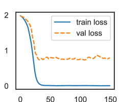
(a) W$\backslash$o re-weigting.

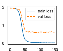
(b) CustomGNN.

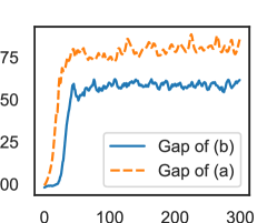
(c) Gap.

Figure 4: (a) is the loss of CustomGNN without path re-weighting, and (b) is the loss of CustomGNN. X-axis denotes training epochs, Y-axis denotes loss values. (c) illustrates the gap between train loss and validation loss of (a) and (b), Y-axis denotes the gap value.

4.5.4 Robustness Analysis

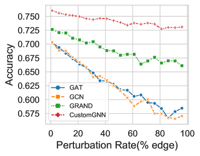
(a) Robustness analysis.

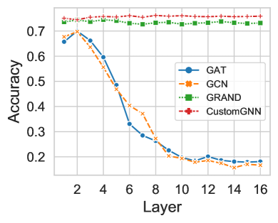
(b) Over-smoothing analysis.

Figure 5: The analysises on Citeseer. On Robustness analysis (a), we gradually increase the perturbation rate (from 1% to 100%). On over-smoothing analysis (b), for GAT, GCN, and GRAND, we increase the propagation layers; For CustomGNN, we increase the propagation layers of multi-hop GNN module, and increase the aggregation orders (window size) of path re-weighting module meanwhile.

We made a noise identification ability and robust analysis of CustomGNN by randomly adding a certain proportion of fake edges. In Figure 5(a), we can observe that the classification accuracy of nodes in GCN and GAT declines rapidly with the increase of fake edges. Although both CustomGNN and GRAND can maintain a slower decline rate in classification accuracy as the number of fake edges increases, CustomGNN is always superior than GRAND in robustness, and the decline curve is smoother.

4.5.5 Over-Smoothing Analysis

Lots of GNN models suffer from the over-smoothing problem. As reported in previous works [13, 18, 47], with the increase of layer numbers, the identification of nodes in different classes become undistinguished, because the multiple propagation steps lead to over-mixing of information and noises [47], then, the node embeddings become similar. Figure 5(b) proved the ability of our model to relieve over-smoothing.

5 Conclusions

In this work, we study the graph neural network from a new view, i.e., customizing GNN for a specific downstream task, and present the Customized Graph Neural Network with Path Reweighting (CustomGNN) which can also resolve the inherent issues of traditional GNNs, such as over-smoothing and over-fitting. In CustomGNN, we capture customized semantic information from weighted paths, which is then infused with a multi-hop GNN model. Moreover, we generate multi-perspective subgraphs to regularize the model and enhance the semantics of features by triplet loss with pseudo-labels. Extensive experiments show that CustomGNN outperforms most SOTAs. In addition, we analyze the semantics learned by CustomGNN and demonstrate the superiority of CustomGNN in terms of resistance to over-smoothing and robustness to data attack. In future work, we aim to apply the impressive semantic extraction ability of CustomGNN to more graph-based tasks.

Appendix A Reproducibility

A.1 Implementation Details

We use PyTorch to implement CustomGNN and all of its components. The LSTM we used in path re-weighting module are implemented in package of torch.nn.LSTM. For the results of large datasets we reported (in Table 4), the implementation of GRAND comes from its public source code, the implementations of GCN and GAT layer come from the PyTorch-Geometric library, and the results of P-reg are taken from its original paper directly. We adopt Adam to optimize parameters of all models in our paper and we perform early stopping strategy to control the training epochs. We employee Dropout in the adjacency matrix, path-weight matrix, encoder, and each layer of prediction module (i.e., MLP) as a general used trick for preventing overfitting. The experiments of Cora, Citeseer are conducted on NVIDIA GeForce RTX 3070 Ti with 8GB memory size, the experiments of PubMed, Cora Full, Amazon Computer, Amazon Photo and Cauthor CS are conducted on Tesla V100 with 32GB memory size. As for software version, we use Pyhton 3.8.5, PyTorch 1.7.1, NumPy 1.19.2, CUDA 11.0.

A.2 Hyperparameter Details

We show the hyperparameters of CustomGNN for results in Table 3. These hyperparameters can be divided into 4 groups, the first controls the training process which are shown in 1 to 12 rows of Table 7, the second controls the customized attention module which are shown in 13 to 16 rows of Table 7, the third controls the triplet loss which are shown in 17 to 20 rows of Table 7, and the fourth control the the consistency loss which are shown in 21 to 22 rows of Table 7.

Hyperparameters	Cora	Citeseer	PubMed
Learning rate $\eta$	0.01	0.01	0.1
Dropout rate of MLP layers	0.5	0.5	0.8
Dropout rate of encoder	0.6	0.6	0.5
Dropout rate of Path Weight Adjacency matrix	0.6	0.6	0.6
Dropout rate of Adjacency matrix	0.5	0.5	0.5
LSTM hidden units	128	128	128
Early stop epochs	300	200	100
L2 weight decay rate	5e-4	5e-4	5e-4
Triplet loss coefficient $\lambda_{1}$ in Eq (5)	1.0	1.0	1.0
Consistency loss coefficient in Eq (5)	1.0	1.0	1.0
Tradeoff $\lambda$, $\dot{\mathbf{F}}\oplus\lambda\hat{\mathbf{F}}$	1.0	10.0	1.0
Embedding dimension (output dimension of Encoder)	512	512	500
Batch size of path sampling	300	300	500
Path length of path sampling	10	10	6
Window size of path sampling	10	5	5
Orders/Layers of Multi-hop GNN module	8	4	5
Number of negative sampling for triplet loss	5000	10000	5000
Number of positive sampling for triplet loss	15000	10000	5000
Margin of negative samples for triplet loss	0.1	1	1
Temperature of consistency loss $T$	0.5	0.5	0.2
Times for regularization $S$	4	4	4

Table 7: Hyperparameters of CustomGNN for reproducing the results reported in Table 3.

Appendix B Additional Experiments

B.1 Dimensional Reduction Analysis

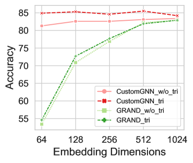
(a) Cora.

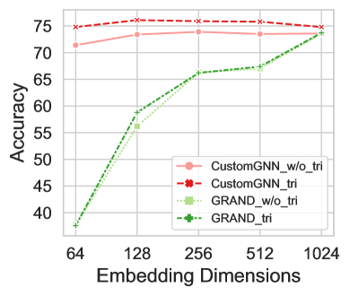
(b) Citeseer.

Figure 6: Analysis of dimension on Cora and Citeseer.

In reality, many nodes attach some auxiliary information, for example, each node on Cora-Full attaches a feature with 8710-dimension. Therefore, the high dimensional features expect low dimensional representations. In this experiment, we conduct encoder $f_{enc}$ to reduce the feature dimension in the beginning, then, CustomGNN is compared with GRAND in different dimensions. As shown in Figure 6, with the decrease of dimension, the accuracy of GRAND declining, however, the accuracy of CustomGNN is stable. The result demonstrates that CustomGNN is not sensitive to different embedding dimensions.

B.2 Weight Correlations Analysis on Citeseer

Figure 7 reports the result of weight correlations analysis on Citeseer, from which we can get the same results as Cora (Section 4.5.2). The settings of Figure 7 are same as Section 4.5.2.

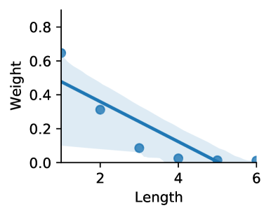
(a) Weight-Length.

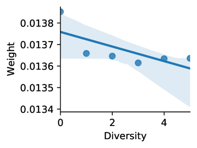
(b) Weight-Diversity.

Figure 7: Analysis of weight correlations on Citeseer.

References

- Gori et al. [2005] M. Gori, G. Monfardini, F. Scarselli, A new model for learning in graph domains, in: IJCNN, 2005.
- Yang et al. [2016] Z. Yang, W. W. Cohen, R. Salakhutdinov, Revisiting semi-supervised learning with graph embeddings, in: ICML, 2016, pp. 40–48.
- Kipf and Welling [2017] T. N. Kipf, M. Welling, Semi-supervised classification with graph convolutional networks, in: ICLR, 2017.
- Ding et al. [2018] M. Ding, J. Tang, J. Zhang, Semi-supervised learning on graphs with generative adversarial nets, in: CIKM, 2018, pp. 913–922.
- Xu et al. [2021] M. Xu, H. Wang, B. Ni, W. Zhang, J. Tang, Graphsad: Learning graph representations with structure-attribute disentanglement, in: ICLR, 2021.
- Scarselli et al. [2009] F. Scarselli, M. Gori, A. C. Tsoi, M. Hagenbuchner, G. Monfardini, The graph neural network model, IEEE Transactions on Neural Networks 20 (2009) 61–80. doi:10.1109/TNN.2008.2005605.
- Hamilton et al. [2017] W. L. Hamilton, Z. Ying, J. Leskovec, Inductive representation learning on large graphs, in: NIPS, 2017, pp. 1024–1034.
- Veličković et al. [2018] P. Veličković, G. Cucurull, A. Casanova, A. Romero, P. Liò, Y. Bengio, Graph attention networks, in: ICLR, 2018.
- Wu et al. [2019] F. Wu, A. H. S. Jr., T. Zhang, C. Fifty, T. Yu, K. Q. Weinberger, Simplifying graph convolutional networks, in: ICML, 2019, pp. 6861–6871.
- Chen et al. [2020] M. Chen, Z. Wei, Z. Huang, B. Ding, Y. Li, Simple and deep graph convolutional networks, in: ICML, 2020, pp. 1725–1735.
- Yang et al. [2022] F. Yang, H. Zhang, S. Tao, Semi-supervised classification via full-graph attention neural networks, Neurocomputing 476 (2022) 63–74. URL: https://www.sciencedirect.com/science/article/pii/S0925231221019330. doi:https://doi.org/10.1016/j.neucom.2021.12.077.
- Gilmer et al. [2017] J. Gilmer, S. S. Schoenholz, P. F. Riley, O. Vinyals, G. E. Dahl, Neural message passing for quantum chemistry, in: ICML, 2017, pp. 1263–1272.
- Li et al. [2018] Q. Li, Z. Han, X.-M. Wu, Deeper insights into graph convolutional networks for semi-supervised learning, in: AAAI, 2018, pp. 3538–3545.
- NT and Maehara [2019] H. NT, T. Maehara, Revisiting graph neural networks: All we have is low-pass filters, CoRR abs/1905.09550 (2019).
- Oono and Suzuki [2020] K. Oono, T. Suzuki, Graph neural networks exponentially lose expressive power for node classification, in: ICLR, 2020.
- Feng et al. [2020] W. Feng, J. Zhang, Y. Dong, Y. Han, H. Luan, Q. Xu, Q. Yang, E. Kharlamov, J. Tang, Graph random neural networks for semi-supervised learning on graphs, in: NeurIPS, 2020.
- Verma et al. [2019] V. Verma, M. Qu, A. Lamb, Y. Bengio, J. Kannala, J. Tang, Graphmix: Improved training of gnns for semi-supervised learning, CoRR abs/1909.11715 (2019).
- Zhu and Koniusz [2021] H. Zhu, P. Koniusz, Simple spectral graph convolution, in: ICLR, 2021.
- Zügner et al. [2018] D. Zügner, A. Akbarnejad, S. Günnemann, Adversarial attacks on neural networks for graph data, in: KDD, 2018, p. 2847–2856.
- Zhu et al. [2019] D. Zhu, Z. Zhang, P. Cui, W. Zhu, Robust graph convolutional networks against adversarial attacks, in: KDD, 2019, p. 1399–1407.
- Olivier et al. [2009] C. Olivier, S. Bernhard, Z. Alexander, Semi-supervised learning, Journal of the Royal Statistical Society 172 (2009) 530–530.
- Lu et al. [2021] Y. Lu, Y. Chen, D. Zhao, D. Li, Mgrl: Graph neural network based inference in a markov network with reinforcement learning for visual navigation, Neurocomputing 421 (2021) 140–150. URL: https://www.sciencedirect.com/science/article/pii/S0925231220312583. doi:https://doi.org/10.1016/j.neucom.2020.07.091.
- Yuan et al. [2022] J. Yuan, M. Cao, H. Cheng, H. Yu, J. Xie, C. Wang, A unified structure learning framework for graph attention networks, Neurocomputing (2022). URL: https://www.sciencedirect.com/science/article/pii/S0925231222000832. doi:https://doi.org/10.1016/j.neucom.2022.01.064.
- Perozzi et al. [2014] B. Perozzi, R. Al-Rfou, S. Skiena, Deepwalk: Online learning of social representations, in: KDD, 2014, pp. 701–710.
- Grover and Leskovec [2016] A. Grover, J. Leskovec, node2vec: Scalable feature learning for networks, in: KDD, 2016, pp. 855–864.
- Chiang et al. [2019] W. Chiang, X. Liu, S. Si, Y. Li, S. Bengio, C. Hsieh, Cluster-gcn: An efficient algorithm for training deep and large graph convolutional networks, in: KDD, 2019, pp. 257–266.
- Lee [2013] D.-H. Lee, Pseudo-label: The simple and efficient semi-supervised learning method for deep neural networks, in: ICML, 2013.
- Elezi et al. [2018] I. Elezi, A. Torcinovich, S. Vascon, M. Pelillo, Transductive label augmentation for improved deep network learning, in: ICPR, 2018, pp. 1432–1437.
- Iscen et al. [2019] A. Iscen, G. Tolias, Y. Avrithis, O. Chum, Label propagation for deep semi-supervised learning, in: CVPR, 2019, pp. 5070–5079.
- Yang et al. [2020] H. Yang, K. Ma, J. Cheng, Rethinking graph regularization for graph neural networks, CoRR abs/2009.02027 (2020).
- Hao et al. [2020] Z. Hao, C. Lu, Z. Huang, H. Wang, Z. Hu, Q. Liu, E. Chen, C. Lee, Asgn: An active semi-supervised graph neural network for molecular property prediction, in: KDD, 2020, pp. 731–752.
- Schroff et al. [2015] F. Schroff, D. Kalenichenko, J. Philbin, Facenet: A unified embedding for face recognition and clustering, in: CVPR, 2015, pp. 815–823.
- Rong et al. [2020] Y. Rong, W. Huang, T. Xu, J. Huang, Dropedge: Towards deep graph convolutional networks on node classification, in: ICLR, 2020.
- Deng et al. [2019] Z. Deng, Y. Dong, J. Zhu, Batch virtual adversarial training for graph convolutional networks, CoRR abs/1902.09192 (2019).
- Gao and Ji [2019] H. Gao, S. Ji, Graph u-nets, in: ICML, 2019, pp. 2083–2092.
- Ma et al. [2019] J. Ma, W. Tang, J. Zhu, Q. Mei, A flexible generative framework for graph-based semi-supervised learning, in: NeurIPS, 2019, pp. 3276–3285.
- Zhang et al. [2018] H. Zhang, M. Cisse, Y. N. Dauphin, D. Lopez-Paz, mixup: Beyond empirical risk minimization, in: ICLR, 2018.
- Mcpherson et al. [2001] M. Mcpherson, L. Smith-Lovin, J. M. Cook, Birds of a feather: Homophily in social networks, Annual Review of Sociology 27 (2001) 415–444.
- Hochreiter and Schmidhuber [1997] S. Hochreiter, J. Schmidhuber, Long short-term memory, Neural Computation 9 (1997) 1735–1780.
- Berthelot et al. [2019] D. Berthelot, N. Carlini, I. Goodfellow, N. Papernot, A. Oliver, C. Raffel, Mixmatch: A holistic approach to semi-supervised learning, in: NeurIPS, 2019, pp. 5050–5060.
- Shchur et al. [2018] O. Shchur, M. Mumme, A. Bojchevski, S. Günnemann, Pitfalls of graph neural network evaluation, CoRR abs/1811.05868 (2018).
- Klicpera et al. [2019] J. Klicpera, A. Bojchevski, S. Günnemann, Predict then propagate: Graph neural networks meet personalized pagerank, in: ICLR, 2019.
- Chen et al. [2018] J. Chen, T. Ma, C. Xiao, Fastgcn: Fast learning with graph convolutional networks via importance sampling, in: ICLR, 2018.
- Qu et al. [2019] M. Qu, Y. Bengio, J. Tang, GMNN: graph markov neural networks, in: ICML, 2019, pp. 5241–5250.
- Gao et al. [2019] Y. Gao, H. Yang, P. Zhang, C. Zhou, Y. Hu, Graphnas: Graph neural architecture search with reinforcement learning, CoRR abs/1904.09981 (2019).
- Kim and Oh [2021] D. Kim, A. Oh, How to find your friendly neighborhood: Graph attention design with self-supervision, in: ICLR, 2021.
- Chen et al. [2020] D. Chen, Y. Lin, W. Li, P. Li, J. Zhou, X. Sun, Measuring and relieving the over-smoothing problem for graph neural networks from the topological view, in: AAAI, 2020, pp. 3438–3445.