Catastrophic Cooling in Superwinds. II. Exploring the Parameter Space

Abstract

Superwinds and superbubbles driven by mechanical feedback from super star clusters (SSCs) are common features in many star-forming galaxies. While the adiabatic fluid model can well describe the dynamics of superwinds, several observations of starburst galaxies revealed the presence of compact regions with suppressed superwinds and strongly radiative cooling, i.e., catastrophic cooling. In the present study, we employ the non-equilibrium atomic chemistry and cooling package maihem, built on the flash hydrodynamics code, to generate a grid of models investigating the dependence of cooling modes on the metallicity, SSC outflow parameters, and ambient density. While gas metallicity plays a substantial role, catastrophic cooling is more sensitive to high mass-loading and reduced kinetic heating efficiency. Our hydrodynamic simulations indicate that the presence of a hot superbubble does not necessarily imply an adiabatic outflow, and vice versa. Using cloudy photoionization models, we predict UV and optical line emission for both adiabatic and catastrophic cooling outflows, for radiation-bounded and partially density-bounded models. Although the line ratios predicted by our radiation-bounded models agree well with observations of star-forming galaxies, they do not provide diagnostics that unambiguously distinguish the parameter space of catastrophically cooling flows. Comparison with observations suggests the possibility of minor density bounding, non-equilibrium ionization, and/or observational bias toward the central outflow regions.

]Received 2021 April 14; revised 2021 July 14; accepted 2021 July 17; published 2021 November 3

1 Introduction

Galactic-scale ionized gaseous outflows, the so-called “superwinds” as defined by Heckman et al. (1990), are commonly observed in starburst galaxies with extreme star formation activity (McCarthy et al., 1987; Heckman et al., 1987; Fabbiano, 1988; Heckman et al., 1990, 1993; Lehnert & Heckman, 1995, 1996; Dahlem, 1997; Dahlem et al., 1997; Heckman, 2002; Rupke et al., 2002, 2005; Martin, 2005; Veilleux et al., 2005). It has been understood that superwinds are driven by the kinetic and thermal energies deposited into the interstellar medium (ISM) by mechanical and radiative feedback from young massive stars (Abbott, 1982; Leitherer et al., 1992; Hopkins et al., 2012) and supernova (SN) explosions (Thornton et al., 1998; Mac Low & Ferrara, 1999; Scannapieco et al., 2002; Creasey et al., 2013), typically in super star clusters (SSCs; Holtzman et al., 1992; O’Connell et al., 1995; Satyapal et al., 1997; Turner et al., 2003; Melo et al., 2005; Smith et al., 2006; Gilbert & Graham, 2007; Galliano et al., 2008). These superwinds are found to be very common in intermediate- and high-redshift star-forming galaxies (Pettini et al., 2001, 2002; Wilman et al., 2005; Steidel et al., 2010), so they may play a crucial role in enriching the intergalactic medium (IGM) in the early Universe (Nath & Trentham, 1997; Lloyd-Davies et al., 2000; Ferrara et al., 2000; Heckman, 2002).

The kinetic and thermal energies from OB stars displace the surrounding ISM and heat it up to $\sim 10^{7}$ K, which can result in large-scale expanding shells, the so-called “superbubbles” (Castor et al., 1975; Bruhweiler et al., 1980; Mac Low & McCray, 1988; Norman & Ikeuchi, 1989) and the production of diffuse X-ray emission (Chu & Mac Low, 1990; Chu et al., 1995; Magnier et al., 1996; Strickland et al., 2002; Silich et al., 2005; Añorve-Zeferino et al., 2009). Superbubbles have been detected around OB stellar clusters (Cash et al., 1980; Abbott et al., 1981; Cash et al., 1980; Mac Low & McCray, 1988; Oey & Massey, 1995; Dove et al., 2000; Reynolds et al., 2001), as well as in many star-forming galaxies (Veilleux et al., 1994; Heckman et al., 1995; Marlowe et al., 1995; Weiß et al., 1999; Strickland & Stevens, 1999; Heckman et al., 2001; Sakamoto et al., 2006; Tsai et al., 2009). These wind-blown bubbles carry off metal-rich material created by massive stars and SN explosions, and enrich the ISM and IGM with the recently produced metals. The dynamics of superbubbles have been modeled by several authors (e.g. Castor et al., 1975; Weaver et al., 1977; Koo & McKee, 1992a, b; Silich et al., 2005). The theoretical calculations by Weaver et al. (1977) suggested the presence of highly ionized ions such as O vi within the hot interior of the superbubble where the temperature spans the range $\sim 10^{5}$–$10^{6}$ K. Moreover, the analytical study by Silich et al. (2005) hinted at the hard (2–8 keV) X-ray emission from the compact hot thermalized ejecta and the soft (0.3–2 keV) diffuse X-ray emission from the superbubble interior.

The mechanical feedback from stellar winds and supernovae have been modeled using adiabatic fluid flow by a number of authors (Castor et al., 1975; Weaver et al., 1977; Chevalier & Clegg, 1985; Cantó et al., 2000). The adiabatic solutions by Castor et al. (1975) and Weaver et al. (1977) were derived by taking an expanding shell surrounded by the H i and H ii regions of a uniform density that leads to the formation of a bubble. Similarly, the adiabatic steady wind solution by Chevalier & Clegg (1985) was obtained by adopting a continuous freely expanding stationary wind without any ambient medium. The analytical solution of Chevalier & Clegg (hereafter CC85; 1985) describes strong superwinds driven by the kinetic and thermal energies supplied by supernovae and massive stars of a stellar cluster. The CC85 model provided the first approximate analytic solution to the adiabatic hydrodynamic properties of the freely streaming stationary superwinds, indicating that density, temperature, and thermal pressure of the superwind around the SSC decrease with radius $r$ as $\rho_{w}\varpropto r^{-2}$, $T_{w}\varpropto r^{-4/3}$, and $P_{w}\varpropto r^{-10/3}$, respectively, while the wind velocity $u_{w}$ approaches the adiabatic terminal speed $V_{A,\infty}$. The numerical simulations of the CC85 model conducted by Cantó et al. (2000) demonstrated that both the analytic adiabatic solutions and their numerical calculations are fully consistent for spherically symmetric homogeneous winds.

Moreover, the semianalytic numerical studies by Silich et al. (2003) and Silich et al. (2004) explored the impact of strongly radiative cooling, called “catastrophic cooling”, on density, temperature, and velocity of an outflow. In particular, Silich et al. (2004) found that the wind temperature predicted by the radiative solution has a departure from the adiabatic approximation of $T_{w}\varpropto r^{-4/3}$ in massive compact clusters. Moreover, an increase in the ejected gas metallicity $Z$ was found to enhance radiative cooling within the cluster volume (Silich et al., 2004; Tenorio-Tagle et al., 2005). The semianalytic modeling and simulations by Tenorio-Tagle et al. (2007) estimated the locus for catastrophic cooling in the plane of cluster size ($R_{\rm sc}$) versus the mechanical luminosity ($L_{\rm mech}=\frac{1}{2}\dot{M}_{\rm sc}V_{A,\infty}^{2}$), which is a function of the total stellar mass-loss rate ($\dot{M}_{\rm sc}$) and the adiabatic terminal speed ($V_{A,\infty}$).

Recent observations are reported to exhibit signs of catastrophic cooling and the suppression of superwinds and superbubbles in SSCs in several starburst galaxies: M82 (Smith et al., 2006; Westmoquette et al., 2014), NGC 2366 (Oey et al., 2017), NGC 5253 (Turner et al., 2017), where the SSCs are embedded within 1–2 pc, dense, ultracompact, high-pressure gas. Similarly, the the most extreme Green Peas (GPs; Jaskot et al., 2017) show kinematics consistent with suppressed superwinds, contrary to other starbursts. Recent ALMA observations of distant star-forming galaxies reveal the presence of extended [C ii] halos that could also be produced by starburst-driven cooling outflows (Fujimoto et al., 2019, 2020; Pizzati et al., 2020). These starburst-driven strongly cooled outflows could be explained by the radiative solution semianalytically derived by Silich et al. (2003, 2004). More recently, Gray et al. (2019a) investigated the occurrence of catastrophic cooling through hydrodynamic simulations including radiative non-equilibrium cooling, which showed the strong enhancement of highly ionized ions such as C iv and O vi.

In the recent work by Gray et al. (2019a, Paper I), the hydrodynamic simulations with the non-equilibrium atomic chemistry and cooling package maihem (Gray et al., 2015; Gray & Scannapieco, 2016; Gray et al., 2019b) were performed assuming a default solar value for the metallicity $Z$ of the outflow, and a typical mass-loss rate of $10^{-2}$ M_⊙ yr^-1. As found by Silich et al. (2004), Tenorio-Tagle et al. (2005), and Gray et al. (2019b), the metallicity can have a significant role in strongly enhancing radiative cooling. Moreover, the mechanical luminosity, i.e. the mass-loss rate and wind terminal speed can affect the domain of catastrophic cooling (Tenorio-Tagle et al., 2007).

In this paper, we therefore investigate a larger parameter space to explore the effect of metallicity $Z$, mass-loss rate $\dot{M}_{\rm sc}$, and wind terminal velocity $V_{\infty}$ on the behavior of catastrophic cooling and superwind suppression. Although our models are parameterized in terms of $\dot{M}_{\rm sc}$ and $V_{\infty}$, we note that these are the effective values that may result after mass-loading or heating efficiency effects. As in Paper I, we use one-dimensional, spherically symmetric hydrodynamic simulations coupled to radiative thermal functions using the non-equilibrium atomic chemistry and cooling package maihem (Gray et al., 2019a) to run an extensive grid of models. In addition, we also investigate some emission-line diagnostics for these conditions. These are generated by post-processing the maihem models with the cloudy photoionization code.

This paper is organized as follows. Section 2 describes the configuration of our hydrodynamic simulations of superwinds, including the radiative thermal functions, initial and boundary conditions. Section 3 describes the implementation of the photoionization modeling, as well as computing population synthesis models for SSCs. The hydrodynamic results from our maihem simulations are presented in Section 4, followed by the emission lines calculated by cloudy and diagnostic diagrams in Section 5. Our results are compared with observations in Section 6, and are discussed in Section 7. Our conclusions are given in Section 8.

2 Hydrodynamic Simulations

We solve the hydrodynamic equations coupled to the radiative cooling and heating functions using the non-equilibrium atomic chemistry and cooling package maihem (Models of Agitated and Illuminated Hindering and Emitting Media; Gray et al., 2015; Gray & Scannapieco, 2016; Gray et al., 2019b), which is a modified version of the adaptive mesh hydrodynamics code flash v4.5 (Fryxell et al., 2000). We use the directionally unsplit pure hydrodynamic solver (Lee et al., 2009; Lee & Deane, 2009; Lee, 2013) together with the second-order Monotone Upwind-centered Scheme for Conservation Laws (MUSCL)–Hancock scheme (van Leer, 1979) developed for arbitrary Lagrangian Eulerian (ALE) and smoothed particle hydrodynamics (SPH) methods. To avoid odd–even instabilities, we also employ a hybrid type of the Riemann solver (Toro et al., 1994), combining the Roe solver (Roe, 1981) and the Harten–Lax–van Leer–Einfeldt (HLLE) solver (Einfeldt, 1988; Einfeldt et al., 1991). The HLLE solver is a modified version of the HLL solver that is positively conservative under certain wavespeed conditions in order to provide more stable and diffusive solutions in strongly shocked regions.

Following Silich et al. (2004), the equations of hydrodynamics applicable to spherically symmetric superwinds in a steady state with the radiative cooling for a spherically symmetric SSC of radius $R_{\rm sc}$ without accounting for the gravitational attraction from the SSC are:

$$\frac{1}{r^{2}}\frac{d}{dr}\left(\rho_{w}u_{w}r^{2}\right)=q_{m},$$ (1)

$$\rho_{w}u_{w}\frac{du_{w}}{dr}+\frac{dP_{w}}{dr}=-q_{m}u_{w},$$ (2)

$$\frac{1}{r^{2}}\frac{d}{dr}\left[\rho_{w}u_{w}r^{2}\left(\frac{u^{2}_{w}}{2}+\frac{\gamma}{\gamma-1}\frac{P_{w}}{\rho_{w}}\right)\right]=q_{e}-q_{c}+q_{h},$$ (3)

where $r$ is the radial distance, $u_{w}$ the wind velocity, $\rho_{w}$ the wind density, $P_{w}$ the wind thermal pressure, $q_{m}=3\dot{M}_{\rm sc}/4\pi R^{3}_{\rm sc}$ the total mass-loss rate per unit volume, $q_{e}=3\dot{E}_{\rm sc}/4\pi R^{3}_{\rm sc}$ the total energy deposition rate per unit volume, $\dot{M}_{\rm sc}$ the total mass-loss rate, $\dot{E}_{\rm sc}$ the total energy deposition rate, $\gamma=5/3$ the ratio of specific heats, $q_{c}=n_{w}^{2}\Lambda(Z,T_{w})$ the cooling rate per unit volume, $q_{h}=n_{w}\Gamma(Z)$ the heating rate per unit volume, $n_{w}$ the wind number density, $\Lambda(Z,T_{w})$ the cooling function (Raymond et al., 1976; Oppenheimer & Schaye, 2013), $\Gamma(Z)$ the heating function (see e.g. Wolfire et al., 2003; Gnedin & Hollon, 2012; Gray & Scannapieco, 2016; Gray et al., 2019b), $T_{w}$ the wind temperature, and $Z$ the metallicity. We adopt the gamma-law equation of state for an ideal gas, $P_{w}=(\gamma-1)\rho_{w}\epsilon_{w}$, where $\epsilon_{w}$ is the internal energy. This accounts for changes in the mean atomic mass due to evolution of the ionization states of all the species. Outside the SSC ($r>R_{\rm sc}$), $q_{m}$ and $q_{e}$ vanish (CC85). The wind model assumes that radiative thermal effects within the SSC are negligible, so $q_{c}$ and $q_{h}$ vanish at $r<R_{\rm sc}$. Taking $q_{c}=0$ and $q_{h}=0$ at $r>R_{\rm sc}$, we recover the adiabatic solution in CC85 and Cantó et al. (2000). The wind terminal velocity is also defined as $V_{\infty}=(2\dot{E}_{\rm sc}/\dot{M}_{\rm sc})^{1/2}$.

Assuming the wind of a uniform density, solving Eqs. (1)–(3) yields the wind density and pressure at $r>R_{\rm sc}$ away from the SSC (Silich et al., 2004):

$$\rho_{w}=\frac{\dot{M}_{\rm sc}}{4\pi u_{w}r^{2}},$$ (4)

$$\frac{dP_{w}}{dr}=\frac{\dot{M}_{\rm sc}}{4\pi r^{3}}\frac{(\gamma-1)r(q_{h}-q_{c})-2\gamma u_{w}P_{w}}{\rho_{w}(u_{w}^{2}-c_{s}^{2})},$$ (5)

where $c_{s}=(\gamma P_{w}/\rho_{w})^{1/2}=(\gamma k_{\rm B}T_{w}/\mu)^{1/2}$ is the sound speed, $\mu$ the mean mass per wind particle, and $k_{\rm B}$ the Boltzmann constant. Following the stationary wind solution of Silich et al. (2004), at $r=R_{sc}$, the Mach number $M=u_{w}/c_{s}=1$ (CC85), so the wind velocity $u_{w}$ is equal to the sound speed $c_{s}$. Following CC85, the wind velocity is $u_{w}=V_{\infty}/2$ at the cluster boundary $r=R_{sc}$. Eq. (4) implies that the wind density at the cluster boundary should be $\rho_{w}=\dot{M}_{\rm sc}/2\pi V_{\infty}R_{\rm sc}^{2}$. As $c_{s}=u_{w}$ at $r=R_{sc}$, the wind temperature and pressure at the cluster boundary should be $T_{w}=\mu V_{\infty}^{2}/4\gamma k_{\rm B}$ and $P_{w}=\rho_{w}V_{\infty}^{2}/4\gamma$, respectively. These values of the wind density and temperature are used as the boundary conditions at $r=R_{sc}$ in our hydrodynamic simulations as described in the following subsection.

2.1 Initial and Boundary Conditions

The hydrodynamic simulations are computed from $t=0$ until an age of 1 Myr at checkpoint intervals of 0.1 Myr. This final age is long enough to generate a mature outflow, but too short for any appreciable evolution in the SED and stellar population. It describes typical superwinds driven by extremely young starbursts. The hydrodynamic model employs one-dimensional, spherical geometry with the initial radius equal to the SSC $R_{\rm sc}$, which is set to 1 pc in our study. This corresponds to the flow injection radius. The outer boundary is set to 250 pc in our hydrodynamic simulations that covers the expansion of fast winds with high mass-loss rates at their final age. We note that the associated Strömgren spheres are often larger, and the outer boundary in our cloudy models are unlimited in radius (described in § 3). The hydrodynamic models are simulated on a base grid consisting of $N_{x}=512$ blocks that are allowed up to two levels of adaptive mesh refinement. This gives a maximum resolution of 0.244 pc. The adaptive mesh algorithm (paramesh; MacNeice et al., 2000) employed by flash uniformly covers the physical space, whose refinement criterion is an error estimator (Löhner, 1987) that is configured to follow the changes in density, temperature, pressure, and velocity. The ambient medium surrounding the SSC does not have any initial kinematics ($u_{w}=0$).

The initial conditions of the wind velocity, temperature, and density at the cluster boundary for the hydrodynamic simulations are adopted based on the analytic radiative solutions (Silich et al., 2004), which are similar to the CC85 adiabatic solutions. The initial values of the temperature and density in the surrounding regions are set to the temperature $T_{\rm amb}$ – that is determined by photoionization of the SSC – and density $n_{\rm amb}$ of the ambient medium, respectively. The initial wind density $\rho_{w,{\rm sc}}$ and temperature $T_{w,{\rm sc}}$ at the cluster boundary ($r=R_{\rm sc}$) are then calculated by assuming the analytic solution:

$$\rho_{w,{\rm sc}}=\frac{\dot{M}_{\rm sc}}{4\pi R_{\rm sc}^{2}u_{w,{\rm sc}}},$$ (6)

$$T_{w,{\rm sc}}=\frac{1}{\gamma}\frac{\mu}{k_{\rm B}}u_{w,{\rm sc}}^{2},$$ (7)

where $u_{w,{\rm sc}}$ is the wind velocity at $r=R_{\rm sc}$ given by the wind terminal speed $V_{\infty}$ (Chevalier & Clegg, 1985; Cantó et al., 2000):

$$u_{w,{\rm sc}}=\tfrac{1}{2}V_{\infty}.$$ (8)

We initialize the boundary wind velocity to $V_{\infty}/2$. This initial wind velocity configuration is based on the wind terminal speed that easily allows us to compare the radiative solution to the adiabatic solution. For the effective area of the outflow $\Omega R^{2}_{\rm sc}$ in Eq. (6), we use $\Omega=4\pi$ corresponding to a fully isotropic outflow, while Gray et al. (2019a) adopted $\Omega=\pi$ describing an anisotropic broken outflow extended perpendicularly to the galactic plane.

Following the CC85 adiabatic solutions, the wind velocity at $r=R_{\rm sc}$ is assumed to be equal to the local sound speed, $u_{w,{\rm sc}}=c_{s,\rm sc}$, which corresponds to a Mach number of 1. The wind terminal speed $V_{\infty}$ is related to the mechanical luminosity as

$$L_{\rm mech}=\tfrac{1}{2}\dot{M}_{\rm sc}V_{\infty}^{2}.$$ (9)

After setting the initial temperature and density from the assumed ambient density, the thermal pressure and internal energy are determined by solving equations (1)–(3) in maihem, using the equation of state. Thus, the wind solution develops from these initial conditions.

The initial thermal pressure derived from the hydrodynamic simulation is found to be consistent with the analytically derived initial pressure:

$$P_{w,{\rm sc}}=\frac{1}{\gamma}\frac{\dot{M}_{\rm sc}u_{w,{\rm sc}}}{4\pi R_{\rm sc}^{2}}.$$ (10)

Alternatively, we could employ the initial analytic pressure $P_{w,{\rm sc}}$ and density $\rho_{w,{\rm sc}}$ and determine the initial temperature $T_{w,{\rm sc}}$ by solving the equation of state in maihem that would provide the same analytic temperature given in Eq. (7). The internal energy per unit mass can also be calculated from the internal pressure and density as follows:

$$\epsilon_{w,{\rm sc}}=\frac{1}{(\gamma-1)}\frac{P_{w,{\rm sc}}}{\rho_{w,{\rm sc}}},$$ (11)

which is calculated by solving the equation of state in maihem. The internal and kinetic energies per unit mass are used to initialize the total energy per unit mass at the cluster boundary ($E_{w,{\rm sc}}=\epsilon_{w,{\rm sc}}+\frac{1}{2}|u_{w,{\rm sc}}|^{2}$).

Following Gray et al. (2019a, b), the gas ejected by the cluster at $R_{\rm sc}$ is approximated to be in collisional ionization equilibrium (CIE) at the boundary, so it depends only on the initial wind temperature and ionizing UV background. The photoionization code cloudy is called to generate the CIE ionization fractions that are a function of temperature and applicable ionizing UV background. Our procedure makes tabulated grids of ionization fractions for all the ions in CIE that span the temperature range of $10^{2}$–$10^{8}$ K, which are linearly interpolated over to yield the ionization fractions at the outflow boundary for a given temperature during our hydrodynamic simulation. The tabulated grids incorporate all the processes considered by cloudy, including collisional excitations, recombination, and collisional ionization. The ionization fractions of the ejected gas at the outflow boundary are then calculated by maihem at runtime through an interpolation on the CIE tabulated grids generated by cloudy.

Table 1 summarizes the parameters used in our maihem hydrodynamic simulations that includes the metallicity used in maihem simulations ($Z$), the mass-loss rate ($\dot{M}_{\rm sc}$), and the wind terminal speed ($V_{\infty}$) in the first three columns. It also lists the metallicities used in Starburst99 models for the Geneva-Rot stellar evolution, high-resolution spectra, and UV spectrum (columns 4–6). The last three columns present Starburst99 outputs: the total luminosity ($L_{\rm tot}$), the fraction of ionizing photons in the H i continuum relative to the total luminosity, $f($H${}^{+})$, and the ionizing luminosity $L_{\rm ion}$. We consider the gas metallicity of $\hat{Z}\equiv Z/$Z${}_{\odot}=1$, $0.5$, $0.25$, and $0.125$, where $Z/$Z${}_{\odot}=1$ corresponds to the ISM abundances listed in Table 2. We adopt the typical ISM abundances of Savage et al. (1977), together with the ISM gas-phase oxygen abundance of Meyer et al. (1998), as the baseline solar metallicity (see Table 2). Typical ISM grains with a dust-to-metal mass ratio of $M_{\rm d}/M_{\rm Z}=0.2$ are incorporated into our initial models of the ionization fraction computed by cloudy  (see also § 3). Dust grains are not included as a distinct species in the maihem simulations, but we use C/O ratios that account for depletion as described in § 3. For the fiducial models with the solar metallicity ($Z/$Z${}_{\odot}=1$), we calculate the boundary density $\rho_{w,{\rm sc}}$ and temperature $T_{w,{\rm sc}}$ using the total mass-loss rate $\dot{M}_{\rm sc}$ of $10^{-1}$, $10^{-2}$, $10^{-3}$, and $10^{-4}$ M_⊙ yr^-1, and the wind terminal speed $V_{\infty}$ of 250, 500, and 1000 km s^-1. For the models with sub-solar metallicities, namely $Z/$Z${}_{\odot}=0.5$, $0.25$, and $0.125$, we scale the mass-loss rates and wind velocities of the solar models according to $\dot{M}_{\rm sc}\varpropto Z^{0.72}$ (Mokiem et al., 2007) and $V_{\infty}\varpropto Z^{0.13}$ (Vink et al., 2001), since we are interested only in extremely young, pre-supernova SSCs that are dominated by stellar winds.

For the ambient medium in our maihem simulations, we adopt the photoionized temperature structure created by the ionizing SED from the parent SSC. This is done using a single cloudy model applied to the density profile predicted by maihem from a preliminary simulation, for the fiducial age of 1 Myr, described in detail § 3.1 (the “PI model”). This sets the ionized radius for the final maihem model, and determines how long the outflow expands into an ionized medium. For most models, the ambient medium remains ionized at 1 Myr. For optically thick models transitioning to a neutral ISM (see §5), which are mostly those with $n_{\rm amb}=10^{3}\ \rm cm^{-3}$, we adopt an ambient temperature of $T_{\rm amb}=5\times 10^{3}$ K. The ionizing SED is generated by the Starburst99 population synthesis model described in § 3 for the fiducial model of $M_{\star}=2.05\times 10^{6}$ M_⊙ at age 1 Myr. This SED is also included as a background UV radiation field in the maihem simulation by using a simple $r^{-2}$ decrease in flux. maihem does not calculate detailed radiative transfer, but since the wind is low density and therefore optically thin, this is a reasonable assumption. Initially, the entire surrounding domain outside the SSC is assumed to have ambient densities of $n_{\rm amb}=1$, $10$, $10^{2}$, and $10^{3}$ cm^-3.

Table 1: Summary of Parameters in Hydrodynamic Simulations by maihem and Stellar Population Models by Starburst99.

Hydro	maihem Outflow Parameters		Starburst99 Inputs			Starburst99 Output
$Z$	$\dot{M}_{\rm sc}(\varpropto Z^{0.72})$	$V_{\infty}(\varpropto Z^{0.13})$	$Z$	$Z$	$Z$	$\log L_{\rm tot}$	$f($H${}^{+})$	$\log L_{\rm ion}$
(Z⊙)	(M⊙ yr-1)	(km s-1)	Geneva-Rot	High Res.Spec.	UV Spec.	(erg s-1)		(erg s-1)
1.0	1.0 $\times$ [$10^{-1}$, $10^{-2}$, $10^{-3}$, $10^{-4}$]	[250, 500, 1000]	0.014	0.020	Solar	42.97	0.41	42.58
0.5	0.607 $\times$ [$10^{-1}$, $10^{-2}$, $10^{-3}$, $10^{-4}$]	[229, 457, 914]	0.008	0.008	LMC/SMC	42.97	0.42	42.60
0.25	0.369 $\times$ [$10^{-1}$, $10^{-2}$, $10^{-3}$, $10^{-4}$]	[209, 418, 835]	0.008	0.008	LMC/SMC	42.97	0.42	42.60
0.125	0.224 $\times$ [$10^{-1}$, $10^{-2}$, $10^{-3}$, $10^{-4}$]	[191, 382, 736]	0.002	0.008	LMC/SMC	42.98	0.50	42.67

• Note. The ambient temperature ($T_{\rm amb}$) is set to the value calculated by the cloudy model for the given Starburst99 SED. Other maihem parameters are as follows: the cluster radius $R_{\rm sc}=1$  pc, the ambient density $n_{\rm amb}=1$, $10$, …, $10^{3}$ cm^-3, the number of blocks $N_{x}=512$, and time intervals $t=0.1$, 0.2, …, $1.0$ Myr. Other Starburst99 parameters are as follows: the total stellar mass $M_{\star}=2.05\times 10^{6}$ M_⊙, and age $t=1$ Myr.

2.2 Non-equilibrium Cooling Functions

To include hydrodynamic heating and background UV radiation, the cooling and heating functions of atomic species are calculated using non-equilibrium ionization (NEI) conditions. The cooling rate per volume $q_{c}(Z,T_{w})$ is determined by the maihem  cooling routine using the cooling function $\Lambda(Z,T_{w})$ based on the gas metallicity $Z$, in addition to the gas temperature $T_{w}$ found by hydrodynamic solutions for given physical conditions and background radiation. We use the cooling routine implemented by Gray et al. (2015), which extended the ion-by-ion cooling efficiencies $\Lambda_{i}(T_{w})$ of Gnat & Ferland (2012) down to 5000 K, for the given ions. Additionally, Gray et al. (2015) included NEI in maihem, which can track non-equilibrium ionization and recombination of species. Furthermore, as fully described by Gray et al. (2019b), the maihem package takes account of the heating rate per volume, $q_{h}(Z)$, by calculating the heating function $\Gamma(Z)$ for the outflow of metallicity $Z$. This atomic chemistry was implemented by incorporating collisional ionization rates (Voronov, 1997), radiative recombination rates (Badnell, 2006), and dielectronic recombination rates (see Table 1 in Gray et al., 2015). With the inclusion of the atomic chemistry package, our simulations are performed using the multispecies extension for the equation of state that accounts for the change in average atomic weight on the thermodynamic quantities. The species and non-equilibrium cooling were incorporated into maihem. These two capabilities, namely non-equilibrium ionization and radiative thermal function allow us to use maihem to investigate the radiative solution of the superwind model.

The package maihem computes the photoionization and photoheating rate for each ion (Verner & Yakovlev, 1995; Verner et al., 1996) to include the effect of an ionizing UV background (Gray & Scannapieco, 2016). The most recent version of maihem updated by Gray et al. (2019b) is able to track non-equilibrium ionization and recombination of 84 species across 13 elements, namely hydrogen (H i–H ii), helium (He i–He iii), carbon (C i–C vii), nitrogen (N i–N viii), oxygen (O i–O ix), neon (Ne i–Ne xi), sodium (Na i–Na vi), magnesium (Mg i–Mg vi), silicon (Si i–Si vi), sulfur (S i–S vi), argon (Ar i–Ar vi), calcium (Ca i–Ca vi), and iron (Fe i–Fe vi). The cooling efficiencies of the new ions in the expanded network of Gray et al. (2019b) were computed using cloudy, in addition to the method used by Gray et al. (2015). The tabulated grids of cooling efficiencies are read into maihem  during the initialization for each model. The latest version models include the column densities of N v and O vi (Gray et al., 2019b).

As mentioned in Gray et al. (2019a), the cooling efficiency $\Lambda_{i}(T_{w})$ of species $i$, the number density $n_{i}$ of species $i$, and the number of electrons $n_{e}$ yield the cooling rate per volume:

$$q_{c}(Z,T_{w})=n_{w}^{2}\Lambda(Z,T_{w})=\sum_{i}n_{i}n_{e}\Lambda_{i}(T_{w}),$$ (12)

which is used in the computations of fluid models to provide radiative cooling. As the ion-by-ion cooling efficiencies $\Lambda_{i}(T_{w})$ are calculated based on the temperature determined by the hydrodynamic simulations for specified physical conditions and background radiation, we see how the mechanical feedback (via $\dot{M}_{\rm sc}$ and $V_{\infty}$) can lead to the catastrophic cooling regime. Furthermore, the cooling function $\Lambda(Z,T_{w})$ is a function of the metallicity specified for the ejected gas.

The heating rate per volume is calculated using the photo-heating efficiency $\Gamma_{i}$ and number density $n_{i}$ of species $i$ as follows (Gray et al., 2019b):

$$q_{h}(Z)=n_{w}\Gamma(Z)=\sum_{i}n_{i}\Gamma_{i},$$ (13)

where the ion-by-ion photo-heating efficiencies $\Gamma_{i}$ are estimated by maihem (see Gray & Scannapieco, 2016) using a background UV spectral energy distribution (SED) and the photoionization cross section of species $i$, taken from Verner & Yakovlev (1995) and Verner et al. (1996).

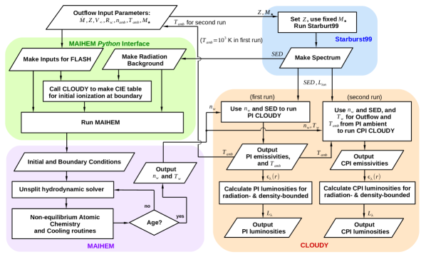
Figure 1: Flowchart of the maihem-cloudy interface implemented in our hydrodynamic simulations. Starburst99 produces the radiation spectrum for the total stellar mass ($M_{\star}=2.05\times 10^{6}$ M_⊙) and given metallicity ($Z$), which is used by maihem and cloudy. The maihem python interface calls cloudy to generate the CIE tables as a function of temperature for the cluster boundary, and produce the background UV SED from the Starburst99 synthetic stellar spectrum to be used by NEI atomic chemistry and cooling routines in maihem. Solving the hydrodynamic fluid equations, together with radiative cooling and heating functions, maihem produces the outflow temperature ($T_{w}$), density profile ($n_{w}$), and NEI states according to the Starburst99 UV SED. The PI cloudy model (pure photoionization) uses only the density profile made by the first maihem hydrodynamic run with an isothermal ambient temperature of $10^{3}$ K, together with the SED model produced by Starburst99. The ambient temperature profile ($T_{\rm amb}$) predicted by the PI cloudy model is employed for the ambient medium in the second maihem hydrodynamic run and the CPI case. The CPI cloudy model (photoionization + hydrodynamic collisional ionization) is calculated in the same way, but uses both the temperature and density profiles of the outflow model produced by the second maihem run, and the ambient temperature structure from the PI model. The radiation- and density-bounded luminosities $L_{\lambda}$ are calculated from the emissivities $\epsilon_{\lambda}(r)$ produced by the PI amd CPI cloudy models, described in Appendix A.

3 Photoionization Calculations

We next carry out photoionization modeling to calculate emissivities of a set of UV/optical emission lines that are typically used for diagnostic purposes. These are used to build diagnostic diagrams (§ 5.1), which we compare with observations (§ 6). The photoionization modeling is implemented as post-processing using the program cloudy v17.02, which is described by Ferland et al. (1998, 2013, 2017). The outflow temperature $T_{w}$ and density $n_{w}$ as a function of the radius $r$ obtained from our hydrodynamic simulations are used as inputs to our photoionization models. Additionally, the SED of the SSC generated by Starburst99 (Leitherer et al., 1999, 2014), together with its predicted ionizing luminosity, as described in § 3.1, is used as an ionizing source for our photoionization models. The stellar evolution and atmosphere models employed by Starburst99 use different increments in metallicity, and so the metallicity in each of our photoionization models is set to the closest match with the metallicity $Z$ (i.e., $Z/$Z${}_{\odot}=1$, $0.5$, $0.25$, and $0.125$) used in the corresponding hydrodynamic simulation, as shown in Table 1.

Similar to Gray et al. (2019a), we model the ionization states for two cases using the same hydrodynamically generated density distribution from maihem: a purely photoionized model based on resetting the entire gas distribution to neutral temperature, and therefore without any hydrodynamic thermal contributions (PI case); and a model with both photoionization and hydrodynamic collisional ionization (CPI case), based on the maihem temperature distribution. These are analogous to models B and C in Paper I. We use a single Cloudy model to generate a more realistic ionization structure, although it is necessarily CIE, since Cloudy cannot model non-CIE. We summarize these models as follows (Figure 1):

1. PI case: This model is only used to generate inputs for the CPI case. The ambient temperature in maihem is initially set to an isothermal value of 1000 K to estimate initial density profiles. Together with the ionizing SED and luminosity from Starburst99, they are employed by cloudy to calculate the photoionization and emissivities due to the stellar radiation of the SSC. The cloudy calculations stop when the temperature drops below 950 K. The resulting temperature profile in the PI case is then used to obtain the photoionized radius and mean ambient temperature for the ionized portion of the ambient medium and shell in the CPI case (see below, and Section 2.1).

2. CPI case: Both the density and temperature profiles generated by maihem together with the ionizing SED and luminosity produced by Starburst99 are used by cloudy to compute the ionization states and emissivities resulting from both the stellar radiation of the SSC and thermal contributions from the hydrodynamic outflow (see Figure 1). The temperature profile found in the PI case is applied to the ambient medium and defines the radius at which the model transitions to neutral and becomes optically thick. The mean ambient ionized temperature in the PI case is adopted for running the maihem model. It is also adopted for the temperature in the ambient medium surrounding the shell, as well as the ionized, isothermal region of the shell, roughly $\sim 1$–2 pc outward from the shell inner boundary. The CPI calculations stop according to the optical depth (H⁺) defined by the PI model.

Thus, the PI cloudy model is used to define the ambient temperature profile in the ambient medium for the hydrodynamic simulation by maihem (see § 2), as well as the ambient medium in the CPI cloudy model. The maihem simulation produces the non-equilibrium ionization states and temperature profile of the outflow. However, we only employ the temperature profile generated by maihem for the CPI model, and not the ionization states, so our cloudy models calculate only CIE conditions. NEI conditions, which can be estimated by including both the ionization states and temperature structure predicted by maihem, generate higher fluxes in certain highly-ionized lines such as C iv and O vi, as shown in Paper I. Our CPI models, which combine the thermal effects and density distribution from both the hydrodynamic outflow and photoionization, are the final, realistic models.

Table 2: ISM abundances and depletion factors for cloudy models

Element	$n({\rm X})/n({\rm H})$	$(1-f_{\rm dpl}({\rm X}))$
He	$0.098$	1.0
C	$2.87\times 10^{-4}$	0.4
N	$7.94\times 10^{-5}$	1.0
O	$3.19\times 10^{-4}$	0.6
Ne	$1.23\times 10^{-4}$	1.0
Na	$3.16\times 10^{-7}$	0.2
Mg	$1.26\times 10^{-5}$	0.2
Si	$3.16\times 10^{-6}$	0.03
S	$3.24\times 10^{-5}$	1.0
Ar	$2.82\times 10^{-6}$	1.0
Ca	$4.10\times 10^{-10}$	$10^{-4}$
Fe	$6.31\times 10^{-7}$	$10^{-2}$

• Note. The abundance $n({\rm X})/n({\rm H})$ of the element ${\rm X}$ is by number relative to the hydrogen abundance. The depletion factor $f_{\rm dpl}({\rm X})$ specifies the depletion fraction of the element ${\rm X}$ onto dust grains. The carbon abundance is set in a way to provide $[n({\rm C})(1-f_{\rm dpl}({\rm C})]/[n({\rm O})(1-f_{\rm dpl}({\rm O})]=0.6$, described in text.

For the cloudy models with $Z/$Z${}_{\odot}=1$, we adopt the ISM abundances derived by Savage et al. (1977) and the ISM oxygen abundance by Meyer et al. (1998), together with their metal depletion onto dust grains (see Table 2), the typical ISM grains, and the C/O ratio parameterized by the metallicity. Several observations implied that the C/O ratio depends on the metallicity (e.g., Garnett et al., 1995, 1999). Considering the C/O measurements by Garnett et al. (1999), the C/O ratio correlates with the O/H abundance as $\log{\rm C}/{\rm O}=3.84+1.16\log{\rm O}/{\rm H}$, so we get ${\rm C}/{\rm O}=0.16$ for the Small Magellanic Cloud (SMC; $\log{\rm O}/{\rm H}=-4$, i.e., $Z/$Z${}_{\odot}\sim 1/5$), ${\rm C}/{\rm O}=0.46$ for the Large Magellanic Cloud (LMC; $\log{\rm O}/{\rm H}=-3.6$, i.e., $Z/$Z${}_{\odot}\sim 1/2$), and ${\rm C}/{\rm O}=0.6$ for the local Galactic ISM ($\log{\rm O}/{\rm H}=-3.5$, i.e., $Z/$Z${}_{\odot}\sim 1$). The carbon abundance is configured to yield the depleted C/O ratio associated with the relevant metallicities (see Table 2). We apply the cloudy “metals” command to the models with the metallicities $Z/$Z${}_{\odot}=0.5$, $0.25$, and $0.125$ to scale down the baseline solar abundances of elements heavier than helium. The same metal depletion and adjusted C/O ratios are also incorporated into cloudy models used by maihem  for initializing CIE states of the ejected gas, as well as for metal species used in the NEI calculations by our maihem simulations.

For our cloudy models, we also include the typical ISM grains with a dust-to-metal mass ratio of $M_{\rm d}/M_{\rm Z}=0.2$, which is typically associated with evolved galaxies (De Vis et al., 2019). Previously, the dust-to-gas versus metallicity correlation (see e.g. Hirashita, 1999; Edmunds, 2001) corresponds to $M_{\rm d}/M_{\rm Z}\sim 0.5$. However, the recent study by De Vis et al. (2019) suggested that evolved galaxies with metallicities above $\log{\rm O}/{\rm H}=-3.8$ have a more or less constant dust-to-metal ratio of $M_{\rm d}/M_{\rm Z}\approx 0.214$, while significantly lower values are expected for unevolved galaxies ($\log{\rm O}/{\rm H}<-3.8$). As we do not consider implications of dust grains in this paper, we assume the standard ISM grains having a constant ratio of $M_{\rm d}/M_{\rm Z}=0.2$. The dust grains along with depleted metallic species are included in cloudy models for initializing CIE states of the outflow in maihem, but not in the NEI module.

3.1 Population Synthesis Models

The spectral energy distribution (SED) of the radiation emitted from stars in the SSC plays an important role in producing the ionization states and emission lines. For the ionizing input of our photoionization models, we employ the latest version of the evolutionary synthesis code Starburst99 (Leitherer et al., 1999, 2014) that was optimized for stellar population with various ages (Vázquez & Leitherer, 2005), as well as extended to include rotational mixing effects (Levesque et al., 2012; Leitherer et al., 2014).

We assume the same fixed SSC mass of $2.05\times 10^{6}$ M_⊙ at all metallicities. This $M_{\star}$ corresponds to $\dot{M}_{\rm sc}=10^{-2}$ M_⊙ yr^-1 for the fiducial Starburst99 model with $Z/$Z${}_{\odot}=1$. We use an initial mass function (IMF) having a power-law $dN/dm\varpropto m^{-\alpha}$ with the Salpeter value $\alpha=2.35$ (Salpeter, 1955), over a mass range of 0.5 to 150 M_⊙. We consider the Geneva stellar evolution with stellar rotation (Geneva-Rot) implemented by Levesque et al. (2012) and Leitherer et al. (2014), which incorporates stellar population grids of Ekström et al. (2012); Georgy et al. (2012). and Georgy et al. (2013). We also employ the stellar wind models of Maeder (1990) and the extended Pauldrach/Hillier atmosphere models (Hillier & Miller, 1998; Pauldrach et al., 2001), which are appropriate for the O-type stellar atmospheres. The Starburst99 high-resolution spectra are built using the evolutionary population synthesis by Martins et al. (2005). The different evolution and atmosphere models have varying metallicity, and we use the closest match to the metallicities in our simulations, as summarized in Table 1.

For our stellar population models, we use an age of 1 Myr, corresponding to the fiducial age of our hydrodynamic simulations. Table 1 also lists the input parameters used in our Starburst99 population synthesis calculations that correspond to the fiducial $M_{*}=2.05\times 10^{6}$ M_⊙ at $Z/$Z${}_{\odot}=1$. The stellar population models yield the ionizing luminosities and SED continua that are used as inputs by our cloudy photoionization models for the adopted fixed $M_{\star}$. Table 1 presents the results from the stellar population models generated by Starburst99: the total luminosity ($L_{\rm tot}$), the fraction of ionizing photons in the H⁺ continuum relative to the total luminosity ($f($H${}^{+})$), and the ionizing luminosity ($L_{\rm ion}$). The ionizing luminosity, which is calculated according to the H⁺ fraction and the total luminosity, together with the synthetic stellar spectrum (SED) are used as inputs in our cloudy photoionization modeling. Decreasing the metallicity $Z/$Z_⊙ with the fixed total stellar mass slightly increases the total luminosity, since metal-poor stars are somewhat hotter and more luminous.

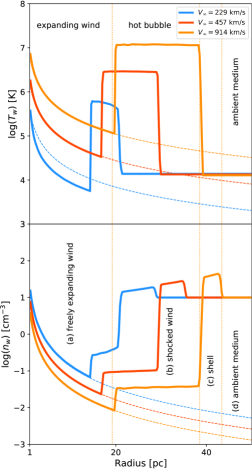
Figure 2: From top to bottom: temperature and density profiles of representative maihem models on a logarithmic scale with ambient density of $n_{\rm amb}=10$ cm^-3, and wind terminal speeds of $V_{\infty}=229$ (blue), $457$ (red), and $914$ km s^-1 (orange solid line). The metallicity is $Z/$Z${}_{\odot}=0.5$ and mass-loss rate $\dot{M}_{\rm sc}=6.07\times 10^{-4}$ M_⊙ yr^-1. The SSC has radius $R_{\rm sc}=1$ pc and age $t=1$ Myr. The different regions separated by dotted lines are labeled for $V_{\infty}=914$ km s^-1: (a) freely expanding wind, (b) shocked-wind, (c) shell, and (d) ambient medium. The adiabatic temperature and density profile for each model are shown by dashed lines. The winds are in the CB (229 km s^-1) and AB ($457$, $914$ km s^-1) modes, described in § 4. The plots for the entire model grid (64 images) are available in the interactive figure in the online journal.

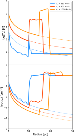
Figure 3: Similar to Figure 2, but showing a catastrophic cooling model with ambient density of $n_{\rm amb}=100$ cm^-3, and wind terminal speed of $V_{\infty}=250\ \rm km\ s^{-1}$ (blue); together with models for $V_{\infty}=500$ (red), and $1000$ km s^-1 (orange solid line). The metallicity is $Z/$Z${}_{\odot}=1$ and mass-loss rate $\dot{M}_{\rm sc}=10^{-3}$ M_⊙ yr^-1. The adiabatic temperature and density profile for each model are shown by dashed lines. The winds are in the CC (250 km s^-1) and AB ($500$, $1000$ km s^-1) modes, described in § 4. The plots for the entire model grid (64 videos) are available in the interactive animation in the online journal.

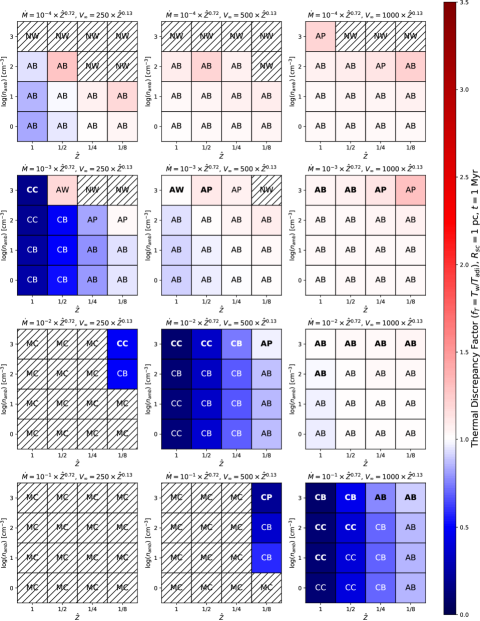
Figure 4: The temperature discrepancy factor ($f_{T}\equiv T_{\rm w}/T_{\rm adi}$) as a function of the metallicity ($\hat{Z}\equiv Z/$Z${}_{\odot}=1$, 0.5, 0.25, and 0.125), the mass-loss rate ($\log\dot{M}_{\rm sc}=-1$, $-2$, $-3$, and $-4$ M_⊙ yr^-1 at $Z=$ Z_⊙) coupled to the metallicity ($\dot{M}_{\rm sc}\varpropto Z^{0.72}$; see Table 1), and the wind terminal velocity ($V_{\infty}=250$, 500, and 1000 km s^-1 at $Z=$ Z_⊙) coupled to the metallicity ($V_{\infty}\varpropto Z^{0.13}$; see Table 1) , and the ambient density ($\log n_{\rm amb}=0$, 1, 2, and 3  cm^-3) computed by the maihem hydrodynamic simulations with the cluster radius of $R_{\rm sc}=1$ pc and the fixed cluster mass of $2.05\times 10^{6}$ M_⊙. The current age of the hydrodynamic iteration is 1 Myr. The wind classification modes based on the temperature profile are presented, namely the adiabatic wind (AW), adiabatic bubble (AB), adiabatic, pressure-confined (AP), catastrophic cooling (CC), catastrophic cooling bubble (CB), catastrophic cooling, pressure-confined (CP), no expanding wind (NW), and momentum-conserving (MC), while the wind modes of the optically thick models are denoted by the bold font.

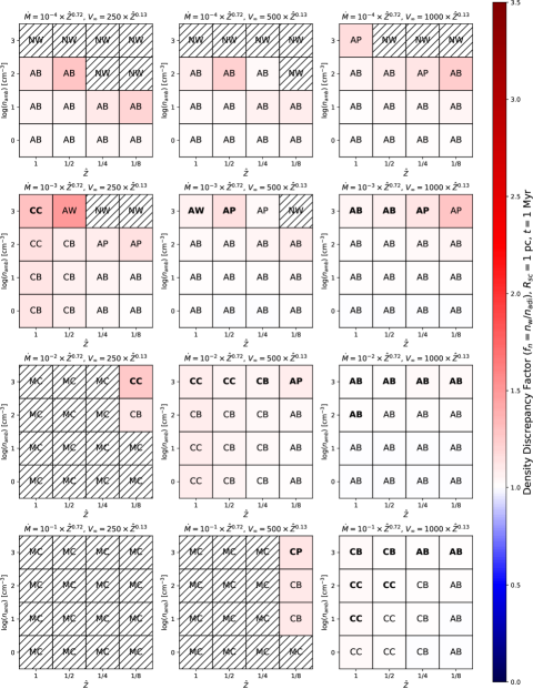
Figure 5: The same as Figure 4, but for the density discrepancy factor ($f_{n}\equiv n_{\rm w}/n_{\rm adi}$)

4 Hydrodynamic Results

In this section, we present the results of our hydrodynamic simulations performed by maihem using the parameters listed in Table 1.

To illustrate different features of the temperature and density profiles in the adiabatic and radiative cooling modes, in Figure 2 we plot the temperature $T_{w}$ and density $n_{w}$ as a function of radius $r$. Considering the hydrodynamic simulations displayed as an example figure at $t=1$ Myr with the metallicity $Z/$Z${}_{\odot}=0.5$, mass-loss rate $\dot{M}_{\rm sc}=6.07\times 10^{-4}$ M_⊙ yr^-1, cluster radius $R_{\rm sc}=1$ pc, ambient density $n_{\rm amb}=10$ cm^-3, and ambient temperature $T_{\rm amb}\sim 1.4\times 10^{4}$ K determined by cloudy: there are two with negligible radiative cooling ($V_{\infty}=457$ and $914$ km s^-1), and one with considerable radiative cooling ($V_{\infty}=229$ km s^-1). The hydrodynamic models ($V_{\infty}=457$ and $914$ km s^-1) without radiative cooling are not continuous freely expanding CC85 winds due to the presence of a shocked-wind region described by Weaver et al. (1977), but possess the CC85 adiabatic solution before the bubble in their temperature and density profiles. The hydrodynamic model ($V_{\infty}=229$ km s^-1) with strongly radiative cooling does not follow the CC85 adiabatic cooling flow before the shell, and it has a radiative solution more similar to that described by Silich et al. (2004).

The adiabatic cooling mode in $V_{\infty}=914$ km s^-1 shown in the example image of Figure 2 has four different regions described in Weaver et al. (1977): (a) freely expanding supersonic wind, (b) shocked wind region, (c) a narrow shell of shocked ambient medium, and (d) the ambient medium. We see that the temperature and density profiles in the region (a) follows the prediction by the CC85 analytic adiabatic solution (dashed line). As the wind propagates into the ambient medium, a hot bubble of shocked wind results, with sharply increased temperature. This leads to the formation of a dense shell due to the confrontation with the ambient medium. The shell has a density higher than the ambient density.

The non-adiabatic, radiative cooling mode is shown in an example figure of Figure 3: this model ($V_{\infty}=250$ km s^-1) has all the regions described in the adiabatic cooling mode, except for the shocked wind region (b) corresponding to the hot bubble. The animated version of this figure shows the evolution for $t=0.1,0.2,\ldots,1$ Myr (available in the online journal). The strong cooling effects suppress the formation of a powerful shocked wind region and an intense temperature bubble. Moreover, the temperature of the freely expanding supersonic wind does not follow the analytic adiabatic solution (dashed line). It can be seen that radiative cooling strongly reduces the temperature of the freely expanding supersonic wind that leads to the deposition of much lower kinetic and thermal energy in the surrounding ambient medium. Thus, we identify three regions in the strongly radiative cooling (catastrophic cooling) mode: freely expanding supersonic wind, a broad shell with density slightly higher than the ambient density, and the surrounding medium. This model corresponds to a momentum-driven shell.

Figure 3 depicts adiabatic cooling with $V_{\infty}=1000$ km s^-1 that does not develop any bubble at ages $t\leq 0.9$ Myr (see its animation in Supplementary Material). However, this model generates a bubble at $t=1$ Myr, so the hot bubble characteristic of the adiabatic solution can take time to develop. In our grid, the model for $V_{\infty}=500$ km s^-1, $n_{\rm amb}=1000$ cm^-3, $Z/$Z${}_{\odot}=1$ at $\dot{M}_{\rm sc}=10^{-3}$ M_⊙ yr^-1 generates bubbles at 1.1 Myr that is greater than the 1 Myr age adopted for all the models. It is important to note that lack of a hot bubble in young objects does not necessarily indicate that the system is strongly cooling or otherwise not adiabatic. Conversely, the hot, shocked wind region can also be present in our simulations at $t=1$ Myr with radiative cooling (e.g. $V_{\infty}=229$ km s^-1 in Figure 2), whose freely expanding wind experiences mildly cooling, but not strong enough to suppress the shocked-wind and hot bubble.

The temperature and density profiles of the superwinds simulated by our hydrodynamic models are therefore classified according to the presence of adiabatic/radiative cooling and the bubble as follows:

1. adiabatic wind (AW) mode: The temperature profile is roughly of freely expanding supersonic winds (CC85) that closely follows the adiabatic solution, and it has not yet produced any bubble, which may develop at a later time. The temperature $T_{\rm w}$ of the expanding wind (region a in Figure 2) produced by maihem is within 0.75 and 1.25 times the temperature $T_{\rm adi}$ analytically derived from the adiabatic solution.

2. adiabatic bubble (AB) mode: This is the classic bubble model (Weaver et al., 1977) where the temperature profile is roughly of adiabatic winds (slightly or without radiative cooling) surrounded by a shocked-wind region (hot bubble; with a thickness $>0.73$ pc and a mean temperature $>10^{5}$ K). The temperature profile closely follows the adiabatic solution of freely expanding supersonic winds (CC85). The temperature $T_{\rm w}$ of the expanding wind computed by maihem  is within 0.75 and 1.25 of the analytic adiabatic temperature $T_{\rm adi}$ over the expanding wind region. The hot bubble (region b in Figure 2) drives the shell expansion.

3. adiabatic, pressure-confined (AP) mode: The expanding wind region is adiabatic, but the bubble expansion is stalled by high ambient pressure from the dense environment. This corresponds to the pressure-confined model predicted by Silich et al. (2007) (also see Koo & McKee, 1992a). The temperature profile is roughly of freely expanding supersonic winds (CC85). The expanding wind temperature $T_{\rm w}$ computed by maihem is between 0.75 and 1.25 times the temperature $T_{\rm adi}$ analytically derived from the adiabatic solution.

4. catastrophic cooling (CC) mode: The temperature profile is of freely expanding winds with strongly radiative cooling (Silich et al., 2003, 2004) without any noticeable shock regions and weak/no bubble. The expanding wind temperature $T_{\rm w}$ of the freely expanding wind (region a) simulated by maihem is at least 25% lower than the temperature $T_{\rm adi}$ analytically derived from the adiabatic solution.

5. catastrophic cooling bubble (CB) mode: The temperature profile has strongly radiative cooling, but still has the bubble and shocked-wind regions. The expanding wind temperature $T_{\rm w}$ of the region (a) is at least 25% below the adiabatic temperature $T_{\rm adi}$ from the analytic solution. Additionally, when the bubble is confined by the high pressure from the ambient medium, we classify it as the cooling, pressure-confined (CP) mode.

6. no wind (NW) mode: The mass-loss rate is extremely low (e.g. $10^{-4}$ M_⊙ yr^-1) and the ambient medium is very dense (e.g. $n=10^{3}$ cm^-3 here), so freely expanding supersonic wind is completely inhibited. The wind solution does not meet the outflow pressure criterion of Cantó et al. (2000) (see below).

7. momentum-conserving (MC) mode: The mass-loss rate is high and the velocity is low, causing catastrophic cooling so that the wind is suppressed. We classify as MC mode those models having a mean initial temperature in region (a) that is a factor of 3 below the expected mean adiabatic temperature within a distance of 1 pc from the cluster boundary.

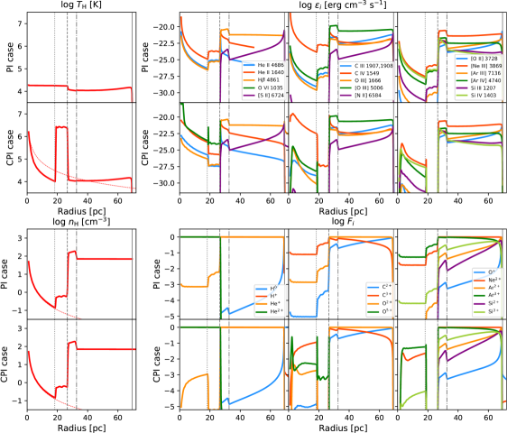
Figure 6: Top Panels: The hydrogen temperature profiles ($T_{\rm H}$ [K]; left panels) along with the adiabatic prediction (red dashed line) in the CPI case, and the line emissivities ($\epsilon_{i}$ [erg cm^-3 s^-1]; right panels) of the superwind models on a logarithmic scale, from top to bottom, in the PI (pure photoionization) and CPI (photoionization $+$ hydrodynamic collisional ionization) cases (§ 3), for wind terminal speed $V_{\infty}=457$ km s^-1, metallicity $\hat{Z}\equiv Z/$Z${}_{\odot}=0.5$, mass-loss rate $\dot{M}_{\rm sc}=0.607\times 10^{-2}$ M_⊙ yr^-1, cluster radius $R_{\rm sc}=1$ pc, and age $t=1$ Myr, surrounded by the ambient medium with density $n_{\rm amb}=100$ cm^-3 and temperature $T_{\rm amb}$ determined by cloudy, producing a wind model in the CB mode (described in § 4). Bottom Panels: The hydrogen density profiles ($n_{\rm H}$ [cm^-3]; left panels) along with the adiabatic prediction (red dashed lines), and the ionic fractions ($F_{i}$; right panels) on a logarithmic scale for the PI and CPI cases. The start and end of the hot bubble (region b), the end of the shell (region c), and the Strömgren radius are shown by dotted, dashed, dash-dotted, and solid lines (gray color), respectively. The plots for all the models (192 images) are available in the interactive figure in the online journal.

The classifications fall into three categories: adiabatic and quasi-adiabatic (AW, AB, AP), radiatively cooling (CC, CB, CP), and suppressed superwinds (NW, MC). The suppressed superwinds are the extreme cases. The NW mode represents the case where the mass-loss rate is too low relative to the ambient density, and a wind cannot launch. As mentioned by Cantó et al. (2000), the existence of the supersonic wind depends on the following outflow pressure:

$$P_{\rm out}\equiv\frac{1}{\gamma}\left(\frac{\gamma-1}{\gamma+1}\right)^{\frac{1}{2}}\left(\frac{\gamma+1}{2}\right)^{\frac{\gamma}{\gamma-1}}\frac{\dot{M}_{\rm sc}V_{\infty}}{4\pi R_{\rm sc}^{2}},$$ (14)

To have the supersonic solution, it is necessary to have the outflow pressure $P_{\rm out}$ higher than the ambient thermal pressure $P_{\rm amb}$ in the surrounding ambient medium. In the ideal gas condition, the ambient thermal pressure $P_{\rm amb}$ is a function of the ambient temperature and density as $P_{\rm amb}=k_{\rm B}T_{\rm amb}\rho_{\rm amb}/\mu$, where $k_{\rm B}$ is Boltzmann’s constant and $\mu$ is the mean mass per particle of the gas. This provides a physical explanation for the dependence of the wind existence upon the mass-loss rate, the wind terminal velocity, and the ambient density, for a given cluster radius ($R_{\rm sc}=1$ pc) and ambient temperature. Outflow with very low mass-loss rate and/or terminal velocity does not support the supersonic solution, so there is no freely expanding supersonic wind. From Eq. (14), it can be seen that supersonic conditions also depend on the cluster radius ($R_{\rm sc}$), so at a very large value of $R_{\rm sc}$, depending on $\dot{M}_{\rm sc}$ and $V_{\infty}$, the existence of freely expanding supersonic winds is also impossible.

Superwinds are also suppressed by the inverse situation where the mass-loss rate is large and the velocity low, causing strong catastrophic cooling. The MC mode corresponds to conditions like these, where there is no significant thermal energy contributing to the outflow, and it roughly proceeds in a momentum-conserving mode only (see e.g. Ostriker & McKee, 1988; Koo & McKee, 1992a, b). For such models with high mass-loss rates and low wind speeds (e.g. $V_{\infty}=250$ km s^-1 for $10^{-2}$ M_⊙ yr^-1), it might often be the case that a supersonic wind cannot be launched at the injection radius $R_{\rm,sc}$ (e.g., Silich & Tenorio-Tagle, 2018). This could arise in situations such as those studied by Silich & Tenorio-Tagle (2018) where hot shocked winds from individual stars strongly cool down inside the cluster before a superwind can be launched into the ambient medium. Previously, it was shown that high mass-loading can contribute to strong radiative cooling in the hot shocked wind (Lochhaas et al., 2018; Silich et al., 2020) that may also suppress or delay the development of a star cluster superwind (Silich et al., 2020).

The parameter space for the different regimes can be seen in Figure 4. This shows the temperature discrepancy factor ($f_{T}\equiv T_{\rm w}/T_{\rm adi}$) defined as the mean value of the expanding wind temperature $T_{\rm w}$ over the predicted analytic adiabatic temperature $T_{\rm adi}\varpropto r^{-4/3}$ for the freely expanding supersonic wind, region (a). A value of $f_{T}$ lower than 0.75 is associated with strongly radiative cooling (CC and CB modes). A value for the temperature discrepancy factor of $\sim 1$ generally corresponds to the adiabatic cooling mode with $0.75<f_{T}<1.25$ (Model AB). It can be seen that, as expected, an increase in the mass-loss rate decreases the temperature discrepancy factor, because the higher density increases cooling. Increasing the metallicity also reduces $f_{T}$, thus also increasing radiative cooling (e.g., Silich et al., 2004). The MC models represent the extreme case, where there is no thermal energy contributing to the outflow. We also see that for a given $\dot{M}_{\rm sc}$, catastrophic cooling occurs for lower outflow velocities. While strong cooling is also promoted by higher metallicity, Figure 4 shows that $\dot{M}_{\rm sc}$ and $V_{\infty}$ are more important over the modeled parameter space.

The pressure-confined models (AP) tend to have higher temperatures, as expected since the adiabatic expansion is reduced, therefore elevating the temperatures in the interior regions according to the ideal gas law. Two models have $f_{T}>1.25$. They are identified in Figure 4 as $\dot{M}_{\rm sc}=10^{-4}$ M_⊙ yr^-1, $V_{\infty}=1000$ km s^-1, $n_{\rm amb}=1000$ cm^-3, $Z/$Z${}_{\odot}=1$; and $\dot{M}_{\rm sc}=0.224\times 10^{-3}$ M_⊙ yr^-1, $V_{\infty}=736$ km s^-1, $n_{\rm amb}=1000$ cm^-3, $Z/$Z${}_{\odot}=0.125$. These are models at the high-density limit, where bubble growth is inhibited the most.

As shown in Figure 5, the density discrepancy factor ($f_{n}\equiv n_{\rm w}/n_{\rm adi}$) defined as the mean value of the expanding wind density $n_{\rm w}$ over the adiabatic density $n_{\rm adi}$ is computed for the freely expanding supersonic wind (region a). It can be seen that the density profiles mostly follow the adiabatic solution. However, the regions with strong cooling (CC, CB) have slightly enhanced densities, as expected. High densities could also lead to high ambient pressures, which also lead to slower bubble growth, sometimes resulting in the adiabatic, pressure-confined (AP) models.

We also see that the wind mechanical power $\frac{1}{2}\dot{M}_{\rm sc}V^{2}_{\infty}$ does not itself determine the outflow’s status with respect to catastrophic cooling; some models with the weakest wind power (upper left group in Figure 4) are still adiabatic. Rather, $\dot{M}_{\rm sc}$ and $V_{\infty}$ are independently the critical parameters in establishing strong cooling. Moreover, we see that there are more catastrophic cooling models that are still capable of supporting hot bubbles (CB) than those without (CC). Thus, the presence of a hot, X-ray superbubble does not necessarily indicate adiabatic feedback.

Figure 4 shows that for the models with fiducial metallicity scalings for the effective mass-loss rate and wind velocity ($\dot{M}_{\rm sc}=10^{-2}$ M_⊙ yr^-1 and $V_{\infty}=1000$  km s^-1), essentially all the models show conventional adiabatic feedback. Reducing $\dot{M}_{\rm sc}$ does not change this scenario until the outflow simply cannot penetrate the ambient density. However, reducing the wind velocity, or otherwise reducing the kinetic heating efficiency, destabilizes these models to catastrophic cooling. Reducing the wind density can mitigate this effect, but only to a point, as seen in these model grids. In practice, regions that tend to be radiation dominated are probably more likely to be mass-loaded due to photoevaporation. A smaller outflow region, which keeps the gas close to the SSC, also promotes these effects. On the other hand, if catastrophic cooling takes place inside the launch radius (e.g., Silich & Tenorio-Tagle, 2018; Silich et al., 2020), it could result in a very small effective $\dot{M}_{\rm sc}\sim 10^{-4}\ \rm M_{\odot}\ yr^{-1}$. This could potentially generate the parameter space of models in that regime, which are otherwise unrealistic for stellar wind outflows.

5 Predicted Emission-Line Ratios

In this section, we present emission line emissivities and luminosities determined using cloudy, for the two different models in § 4, namely, PI (pure photoionization) and CPI (photoionization $+$ hydrodynamic collisional ionization).

Figure 6 (top panels) shows the emissivities calculated for various emission lines as a function of radius for our photoionization models with the two different ionization schemes (PI and CPI; right panels). The PI emissivity profiles, which were made using the Starburst99 SED and luminosity applied to the neutral density profile from the hydrodynamic simulation, are shown in the top panel. The bottom panel presents the emissivities from the CPI model built using both the Starburst99 SED ionizing source and hydrodynamic ionization. Similarly, the ionic fractions for our photoionization models with these two different (PI and CPI) models are presented in Figure 6 (bottom panels).

The CPI models are used to calculate line emissivities in what follows. We classify our photoionization models according to the nebular (H⁺) optical depth of the swept-up shell. Optically thick models are shown with bold-face in Figure 4. Models are optically thin if the ambient medium beyond the shell (region c in Figure 2) is photoionized to produce H⁺ by the SSC. We see that the optically thick models are those in the densest ($n_{\rm amb}\gtrsim 10^{2}$) ambient media, for which dense, optically thick swept-up shells develop more quickly. However, we caution that our 1-D models do not account for shell clumping which can greatly alter the escape fraction of ionizing radiation. We also caution that maihem does not implement radiative transfer, which may be a significant effect in high-density models. Thus, the exact boundary of the ionized edge is approximate, and the ionization structure of the interface region between the optically thin and thick conditions are also approximated. Thus for the optically thick cloudy  models, we adopt the radial temperature profile from the PI model from the radius at which the shell becomes isothermal according to the maihem simulation, roughly 1–2 pc outward from the inner boundary of the dense shell (see Section 3).

Observations of distant, luminous complexes may be biased toward the central, high surface-brightness regions, thereby approximating density bounded observations transverse to the line of sight. To allow for the calculation of partially and fully radiation-bounded models, the total luminosity $L_{\lambda}$ of each emission line at wavelength $\lambda$ is calculated from its volume emissivity $\epsilon_{\lambda}(r)$ as follows (see Appendix A):

$$L_{\lambda}=4\pi\int^{R_{\rm aper}}_{R=0}\left[\int^{R_{\rm max}}_{r=R}\frac{\epsilon_{\lambda}(r)}{\sqrt{r^{2}-R^{2}}}rdr\right]RdR,$$ (15)

where $r$ is the radial distance from the center, $R$ the projected distance from the center, $R_{\rm aper}$ the radius of the circular projected aperture within the object observed, and $R_{\rm max}$ the maximum radius of the object in the line of sight. Thus, for a fully “density-bounded” model, we set $R_{\rm max}=R_{\rm shell}$, i.e., the maximum radius of the dense shell (region c in Figure 2), and $R_{\rm aper}=R_{\rm shell}$. For a fully “radiation-bounded” H ii region, $R_{\rm max}$ and $R_{\rm aper}$ are set to the Strömgren radius $R_{\rm Str}$ predicted by cloudy. Setting $R_{\rm aper}=R_{\rm shell}$ and $R_{\rm max}=R_{\rm Str}$ is radiation bounded in the line of sight, but otherwise density bounded. This geometry is described as a “partially density-bounded” model in what follows. Appendix A fully describes the calculations based on this geometry.

Table 3 partially lists the total luminosities derived from emissivities calculated by cloudy for radiation-bounded, partially density-bounded, and density-bounded models with the two different cases (PI and CPI). The tables for all the photoionization calculations are presented in the machine-readable format in Appendix B.

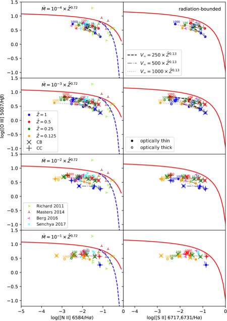
Figure 7: The optical diagnostic BPT diagrams plotted [O iii] $\lambda$5007/H$\beta$ versus [N ii] $\lambda$6584/H$\alpha$ (left) and [O iii] $\lambda$5007/H$\beta$ versus [S ii] $\lambda\lambda$6717,6731/H$\alpha$ (right panels) for the fully radiation-bounded models with mass-loss rates $\log\dot{M}_{\rm sc}=-4$, $-3$, $-2$, and $-1$ M${}_{\odot}/$yr (from top to bottom), ambient densities $n_{\rm amb}=1$, 10, $10^{2}$, and $10^{3}$ cm^-3 (labeled on plots), metallicities $\hat{Z}\equiv Z/$Z${}_{\odot}=1$ (blue), $0.5$ (red), $0.25$ (green), and $0.125$ (yellow color), and wind terminal velocities $V_{\infty}=250$ (dashed), $500$ (dash-dotted), and $1000$ km s^-1 (dotted lines). For the sub-solar models, we use the solar model parameters scaled as $\dot{M}_{\rm sc}\varpropto Z^{0.72}$ and $V_{\infty}\varpropto Z^{0.13}$. The optically thin and thick models are plotted by filled and empty circles, respectively. Line emissivities for optically thick models are somewhat uncertain. The wind catastrophic cooling (CC) and catastrophic cooling with the bubble (CB) modes are labeled by the plus (’$+$’) and cross (’$\times$’) symbols, respectively. The solid (red color) and dashed (blue color) lines show the upper and lower boundaries to star-forming galaxies from Kewley et al. (2001) and Kauffmann et al. (2003), respectively, whereas those above the solid red line are classed as AGN. The plotted observations are from Richard et al. (2011), Masters et al. (2014), Berg et al. (2016), and Senchyna et al. (2017).

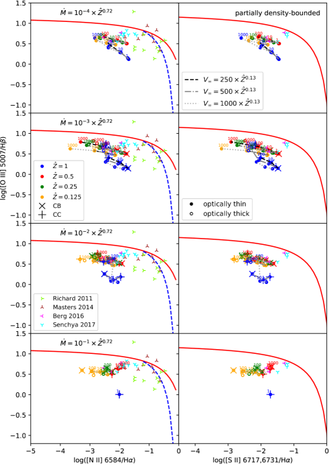
Figure 8: The same as Figure 7, but for the partially density-bounded models.

5.1 Diagnostic Diagrams

Here, we explore the emission-line parameter space generated by our CPI models in a few diagnostic diagrams, including the locus for catastrophic cooling models. We use our total luminosities derived from cloudy emissivities to produce diagnostic diagrams for different metallicities, wind terminal velocities, ambient densities, and mass-loss rates.

Figure 7 shows “BPT diagrams” (Baldwin et al., 1981) based on [O iii] $\lambda$5007/H$\beta$ versus [S ii] $\lambda\lambda$6717,6731/H$\alpha$ and [N ii] $\lambda$6584/H$\alpha$ for our fully radiation-bounded models with optically thin and thick shells plotted by filled and empty circles, respectively. As noted above, given the uncertainties when the transition between optically thin and thick conditions takes place in the shell, the line emissivities for optically thick models are somewhat uncertain. These diagrams are widely used to distinguish between active galactic nuclei (AGN) and starburst galaxies (e.g., Veilleux & Osterbrock, 1987; Osterbrock et al., 1992; Kewley et al., 2001, 2006, 2013; Groves et al., 2004, 2006). Similarly, Figure 8 shows the same models as in Figure 7 but with the emission-line luminosities calculated as density-bounded at the shell outer radius transverse to the line of sight, as described above.

In general, we see that both sets of models in Figures 7 and 8 show line ratios typical of photoionized H ii regions. This applies to both adiabatic and strongly cooling conditions. The models are highly excited, although slightly below the starburst boundaries defined by Kewley et al. (2001) and Kauffmann et al. (2003). This is likely caused by the fact that the ionization parameter is diluted by the outflows in our models, which displace the gas to larger radii at the shells. Higher density models also have higher ionization parameters, as evidenced by their low [N ii] and [S ii] emission. As expected, at higher metallicity, [O iii]/H$\beta$  decreases due to stronger cooling. The partially density-bounded models in Figure 8 are similar to the fully radiation-bounded ones in Figure 7, but lacking the strongest [N ii] and [S ii] emission, which ordinarily dominates in the outer regions. Since the wind itself is more highly ionized and low density, the contributions from kinematic heating are not apparent in the species shown by the BPT diagrams.

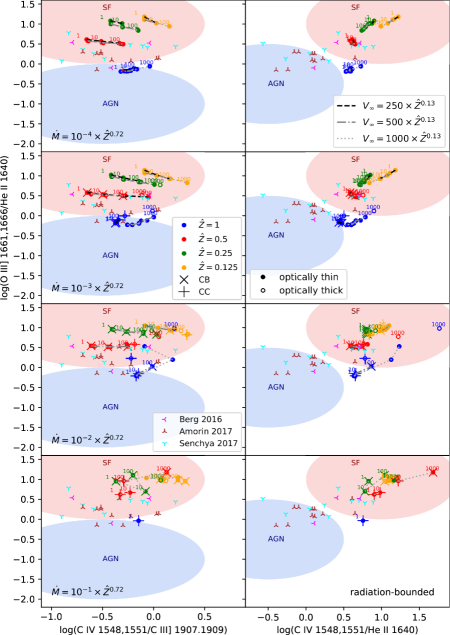
Figure 9: The UV diagnostic diagrams plotted O iii] $\lambda\lambda$1661,1666/He ii $\lambda$1640 versus C iv $\lambda\lambda$1548,1551/C iii] $\lambda\lambda$1907,1909 (left) and O iii] $\lambda\lambda$1661,1666/He ii $\lambda$1640 versus C iv $\lambda\lambda$1548,1551/He ii $\lambda$1640 (right panels). Symbols and line types are as in Figure 7. The red and blue color filled areas represent the approximate regions associated with star-forming (SF) and active (AGN) galaxies from Gutkin et al. (2016) and Feltre et al. (2016), respectively. The plotted observations are from Berg et al. (2016), Amorín et al. (2017), and Senchyna et al. (2017).

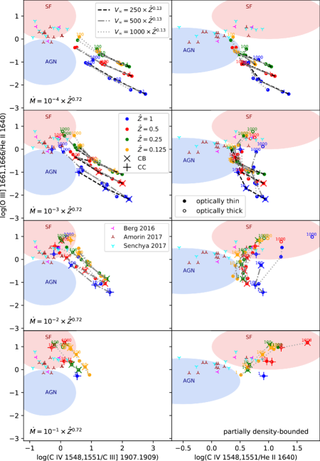
Figure 10: The same as Figure 9, but for the partially density-bounded models.

Similar to the optical BPT diagrams, UV diagnostics diagrams based on ultraviolet emission lines such as C iv $\lambda\lambda$1549,1551, He ii $\lambda$1640, O iii] $\lambda\lambda$1661,1666, C iii] $\lambda\lambda$1907,1909, He ii $\lambda$1640 have been employed to distinguish between AGN and starburst galaxies (Allen et al., 1998; Feltre et al., 2016; Gutkin et al., 2016; Hirschmann et al., 2019), and radiative shock regions (Allen et al., 1998; McDonald et al., 2015; Hirschmann et al., 2019). We select sets of those UV diagnostic line ratios that are typically reported in star-forming regions to make UV diagnostic diagrams. Fully radiation-bounded models are presented in Figures 9 and 11; and models that are density-bounded transverse to the line of sight in Figures 10 and 12.

Figure 9 presents the UV diagnostic diagrams for O iii] $\lambda\lambda$1661,1666/He ii $\lambda$1640 versus C iv $\lambda\lambda$1548,1551/C iii] $\lambda\lambda$1907,1909 and C iv $\lambda\lambda$1548,1551/He ii $\lambda$1640, for our fully radiation-bounded models. In general, these line ratios increase for decreasing metallicity, due to the increasing nebular electron temperature in metal-poor systems. However, at $Z/$Z${}_{\odot}=1$, strong adiabatic feedback generates hot bubbles with strong C iv emission in the interface with the dense shell, displacing some models for $V_{\infty}=1000$ km s^-1 to higher C iv ratios relative to other models. For all other models, the wind heating is unimportant for these emission-line ratios. This highlights the weakness of stellar winds at low metallicity.

These effects are more pronounced in Figure 10, which is the same as Figure 9, but for models that are partially density-bounded. Since these models are weighted toward emission in and near the shell, the C iv emissivity is enhanced in models with significant adiabatic feedback, such as those at lower density and higher velocity. On the other hand, O iii] is more sensitive to the overall electron temperature, which decreases with increasing the ambient density.

The highly ionized doublet O vi $\lambda\lambda$1032,1038 originates from shocks and hydrodynamic collisional ionization, rather than photoionization. Gray et al. (2019b) suggested that it could be a useful diagnostic of catastrophic cooling flows. In Figures 11 and 12, we examine O vi $\lambda\lambda$1032,1038/He ii $\lambda$1640 versus C iv $\lambda\lambda$1549,1551/He ii $\lambda$1640, for fully radiation-bounded, and partially density-bounded transverse to the line of sight, respectively. In our models, the O vi emission is produced primarily in the central region of the free-expanding wind, nearest to the SSC; and in the dense shell interfaces to the hot bubble region (see Figure 6, top panels).

Figures 11 and 12 show that denser winds increase the O vi emission through strong cooling, which correlates strongly with $\dot{M}_{\rm sc}$, as well as showing a slight anticorrelation with $V_{\infty}$. These effects are enhanced in the partially density-bounded plots in Figure 12. This is consistent with the suggestion by Paper I that O vi is associated with catastrophic cooling, but we also see that adiabatic models also show significant O vi. Thus, while O vi is indeed enhanced in most catastrophic cooling models, it is difficult to use as a definitive diagnostic of these conditions without other constraints on the parameter space. Indeed, for the most strongly cooling models, in which the hot bubble region is eliminated, the temperature is too low to generate O vi at all.

We caution that, as demonstrated by Gray et al. (2019b), the O vi emission line can be strong in the outflow due to non-equilibrium ionization states. Moreover, Paper I shows that NEI conditions are expected to contribute to more highly ionized states than in CIE, especially in strongly cooling flows. This is also seen, for example, in supernova remnants (e.g. Patnaude et al., 2009, 2010; Zhang et al., 2019).

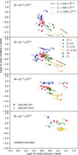
Figure 11: The UV diagnostic diagrams plotted O vi $\lambda\lambda$1032,1038/He ii $\lambda$1640 versus C iv $\lambda\lambda$1548,1551/He ii $\lambda$1640 for the radiation-bounded models. Symbols and line types are as in Figure 7.

Figure 12: The same as Figure 11, but for the partially density-bounded models.

In Figure 7–12, we also see that optically thick models typically appear in denser ambient media. Figure 7 shows that the ambient density of $n_{\rm amb}=10^{3}$ cm^-3 results in weaker singly-ionized emission lines [N ii] and [S ii]. As seen in Figure 9, an increase in the metallicity ($Z/$Z_⊙) mostly tends to decrease the UV line ratios O iii]/He ii and C iv/He ii, since the nebular temperature decreases. It is also not clear that enhanced C iv emission is strongly associated with catastrophic cooling models as suggested in Paper I. However, future work with NEI models are needed to clarify this.

As noted above, our cloudy models include dust grains with $M_{\rm d}/M_{\rm Z}=0.2$ found by De Vis et al. (2019) for evolved galaxies. Dust grains could also form in shocked ejecta from SN explosions (e.g., Nozawa et al., 2010) in starburst-driven superwinds. On the other hand, the dust-to-metal ratio could be lower for unevolved galaxies. Although the optical diagnostic line ratios plotted in the BPT diagrams are not greatly affected by the presence of dust grains, they can have significant changes on the UV line ratios, since dust grains slightly decrease radiation fields. Moreover, metal depletion onto dust grains reduces the ratios of C iv $\lambda\lambda$1549,1551/He ii $\lambda$1640 and O vi $\lambda\lambda$1032,1038/He ii $\lambda$1640. Thus dust grains and depletion onto them are additional sources of uncertainties in these line ratios, as well as in NEI cooling functions (e.g., Richings et al., 2014).

6 Comparison with Observations

We compare our results with optical and UV observations of nearby and distant starburst galaxies, which were found to have detected observations of He ii $\lambda$1640, C iv $\lambda$1550, O iii] $\lambda$1664, and C iii] $\lambda$1908. The observations of low metallicity compact dwarf galaxies studied by Berg et al. (2016) have mean oxygen abundance of $12+\log($O/H$)\approx 7.6$ ($\hat{Z}\approx 0.125$), and electron temperatures $T_{\rm e}($[N ii]$)\approx 15000$ K. Nearby starburst dwarf galaxies studied by Senchyna et al. (2017) have similar parameters, but with $12+\log($O/H$)\lesssim 8.3$ ($\hat{Z}\lesssim 0.6$). More distant starburst galaxies have been extensively analyzed using optical nebular lines, and some have been recently studied through rest-frame UV spectroscopic observations (Stark et al., 2014; Patrício et al., 2016; Steidel et al., 2016; Amorín et al., 2017; Vanzella et al., 2016; Saxena et al., 2020). In particular, Amorín et al. (2017) considered 10 starburst galaxies at redshift $2.4<z<3.5$ with mean metallicity of $12+\log($O/H$)\approx 7.6$, for which they measured Ly$\alpha$ $\lambda$1216, C iv $\lambda$1550, He ii $\lambda$1640, O iii] $\lambda$1664, and C iii] $\lambda$1908. These objects have similar properties and line ratios as the samples of Berg et al. (2016) and Senchyna et al. (2017), and they are also included in Figures 9 and 10. Their properties are largely the same as those of the local sample for the considered line ratios. The galaxy samples occupy the parameter space used for our models, as shown in Figures 7 to 10.

It can be seen in Figures 7 and 8 that, for the appropriate metallicity within $Z/$Z${}_{\odot}=0.125$ and $0.5$, the data agree more with our fully radiation-bounded models than with the partially density-bounded models. This implies that the conditions in these objects do not require significant density bounding for the integrated nebular emission. However, since these apertures are on the order of a few kpc, we note that the observed singly-ionized emission lines could be due to the diffuse interstellar medium, and so some density bounding is not ruled out. These samples have similarities to the Green Pea galaxies, which tend to have higher ionization parameters, with weaker emission from the low-ionization species in Figures 7 and 8.

Figures 9–10 also show the UV observational data from Berg et al. (2016) and Senchyna et al. (2017) plotted on the UV diagnostic diagrams. We again see reasonably good correspondence between the data and models for $Z/$Z${}_{\odot}=0.5$ and 0.25. In Figure 9, the models appear to slightly overpredict O iii]/He ii ratio. For these radiation-bounded conditions, the discrepancy may be due to the CIE approximation in our models. As shown in Paper I, NEI conditions for such outflows generate slightly higher ionization states, which would reduce O iii]/He ii and C iii]/C iv. Furthermore, Figure 10 also shows that only a small degree of density bounding for the high-density models can alleviate the discrepancy. This density bounding could be an observational bias, as suggested earlier; or it could be at least partially real, since similar galaxies have been found to be Lyman-continuum emitters (e.g., Izotov et al., 2016, 2018).

The O vi $\lambda\lambda$1032,1038 emission and absorption lines are more readily associated with active galaxies and AGN feedback, rather than starbursts (e.g., Baldwin et al., 2003; Hainline et al., 2011; Tripp et al., 2008; Savage et al., 2014; Bielby et al., 2019). We do not typically expect O vi emission in ordinary H ii regions, since these highly ionized lines originate from a hot gas phase with $T\sim 3\times 10^{5}$ K. Generally in starbursts, this species is only seen in absorption, associated with adiabatic outflows (e.g., Heckman et al., 2001). But recently, Hayes et al. (2016) spatially resolved O vi $\lambda\lambda$1032,1038 emission in a nearby, intense starburst galaxy (SDSS J115630.63+500822.1, hereafter J1156) through Hubble Space Telescope (HST) imaging, having spectroscopically observed this emission with the Far Ultraviolet Spectroscopic Explorer (FUSE). Moreover, they also detected a blueshifted O vi absorption line associated with an average outflow velocity of $380$ km s^-1. From the O vi column density, they found an O vi mass of $3\times 10^{4}$ M_⊙. The starburst properties of this galaxy are similar to those of our comparison datasets, and it has metallicity $7.87<12+\log($O/H$)<8.34$ (i.e. $0.23<\hat{Z}<0.7$).

Chisholm et al. (2018) confirmed that photoionization models of galactic outflows with cloudy cannot reproduce the observed O vi absorption in a high-redshift starburst, so they again point to the standard model that O vi originates from a mass-loading interface between the photoionized region and unobserved hot wind. However, Gray et al. (2019b) found that NEI models can produce a range of O vi column densities in dense outflows themselves, confirming that relatively high O vi emission can also be due to hydrodynamic heating. Moreover, Paper I also reproduced strong O vi and C iv emission from strongly cooling winds, so they suggested that these lines could be used to trace catastrophically cooling superwinds in starburst regions. In Figure 11, we see that the O vi emission is indeed enhanced by increasing the mass-loss rate and metallicity, and it is typically stronger in catastrophic cooling models. However, the O vi emission plummets in the models at $Z/$Z${}_{\odot}=1$ and $\dot{M}_{\rm sc}$ $=$ $10^{-3}$ M${}_{\odot}/$yr, where strong radiative cooling occurs. Moreover, O vi is also seen in adiabatic models, so additional constraints on the parameter space are necessary when using this line to evaluate the presence of catastrophic cooling.

7 Discussion

The local extreme emission-line galaxies are regarded as analogs of higher redshift starbursts. Various samples of such objects have been reported, and they have similar properties and emission-line ratios as the comparison samples above from Berg et al. (2016) and Senchyna et al. (2017). For example, the recent deep VANDELS spectroscopic survey of He ii emitting galaxies by Saxena et al. (2020) identified 8 objects with high enough SNR at $z\sim 2.5$–3.5 to detect He ii $\lambda$1640, O iii] $\lambda\lambda$1661,1666 lines, and C iii] $\lambda$1909 in emission. The metallicity of these He ii emitters are estimated to be in the range $Z/$Z${}_{\odot}=0.125$ to $0.25$, similar to the low-redshift samples. Other UV observations of intermediate redshift sources have similar physical conditions. Deep spectroscopic observations of low mass, gravitationally lensed galaxies at $z\sim 1.5$–3 conducted by Stark et al. (2014) identified moderately metal-poor gaseous environments with $\sim 0.2$–0.5 Z_⊙, and MUSE integral field spectroscopy of a young lensed galaxy at $z=3.5$ (SMACSJ2031.8-4036) by Patrício et al. (2016) revealed similar physical conditions ($T_{\rm e}\sim 15600$ K) and metallicity ($\lesssim 0.16$ Z_⊙).

These highly excited starbursts appear to be linked to Lyman continuum (LyC) emission. The extreme Green Pea galaxies are to date the only class of objects known to be confirmed LyC emitters (e.g., Izotov et al., 2016, 2018), and they are characterized by their extreme nebular excitation (Cardamone et al., 2009). At intermediate redshift, de Barros et al. (2016) investigated the UV spectrum of a LyC emitter candidate at $z=3.2$, called Ion2, which has $12+\log($O/H$)\approx 8.1$ ($\hat{Z}\approx 0.4$), and strong Ly$\alpha$ [O iii] $\lambda\lambda$4959,5007 and C iii] $\lambda\lambda$1907,1909. Ion2 exhibits an extremely high [O iii]/[O ii] ratio $>10$, which is much higher than expected according to the SFR–$M_{\star}$–$Z$ dependence of [O iii]/[O ii] ratios derived by Nakajima & Ouchi (2014). de Barros et al. (2016) suggest that this could be due to a density-bounded scenario. Indeed, primeval galaxies at the time of cosmic reionization ($z>7$) also have these extreme emission line properties, and similarly are very compact, with high star formation rates and lower masses (e.g., Grazian et al., 2015; Shibuya et al., 2015; Tasca et al., 2015). Stark et al. (2015) analyzed the UV observations of a gravitationally lensed, Ly$\alpha$ emitter at $z=7.045$ (A1703-zd6) and having $12+\log($O/H$)\approx 7.04$. They detected C iv $\lambda$1548 emission with ${\rm FWHM}\lesssim 125$ km s^-1. Although this is similar to measurements in narrow-lined AGNs at lower redshift, it could also originate from a starburst region powered by young, very hot, metal-poor stars.

Catastrophic cooling conditions have been suggested to be present in some of these extreme starbursts (e.g., Silich et al., 2020; Jaskot et al., 2019; Oey et al., 2017) based on kinematic and other evidence. If this is indeed the case, then our results would imply that mostly likely the heating efficiency in these systems is significantly reduced relative to the fiducial scalings for stellar wind velocities (Section 4). It is also possible that mass-loading plays a role, but the degree of mass loading required to induce catastrophic cooling is high. Since these objects tend to be metal-poor, it is unlikely that metallicity plays a significant role in promoting cooling. If this is indeed the case, then our results in Section 4 would imply that either (1) the heating efficiency in these systems is low; (2) mass-loading is high; or (3) the winds are suppressed within the injection radius $R_{\rm sc}$. The first option would imply that the effective wind velocity is reduced by at least a factor of 2–4, since stellar winds are on the order of 1000–2000 km s^-1, even at low metallicity. This would correspond to a decrease in kinetic heating efficiency of 0.25 to 0.06, and could be caused by a variety of factors like entrainment of clouds, turbulence, and magnetic fields. The second option would similarly require an increase in effective $\dot{M}_{\rm sc}$ by an order of magnitude, which could be accomplished by mass-loading. The third option would require both weak velocities and high $\dot{M}_{\rm sc}$ in order to suppress the wind within $R_{\rm sc}$. This has been suggested to be the case in NGC 5253-D1 by Silich et al. (2020).

Thus, our modeled emission-line spectra and outflow parameter space may be relevant to LyC emitters and primordial galaxies. Our comparison with the local extreme starbursts shows that our models for $Z/Z_{\odot}=0.5$ and 0.25 are reasonably good at matching the observed emission-line data for C iv, C iii], O iii], and He ii when invoking a slight density bounding at high ambient densities, on the order of 100 cm^-3. This density bounding would be expected for LyC emitters, although it could also simply be an observational bias favoring the brightest, swept-up gas. Or, as discussed in Section 6, the objects are fully radiation bounded but with NEI conditions in the outflow that cause the modest variation from our modeled emission-line ratios. Both scenarios imply a significant contribution from kinematic heating to generate the observed high ionization states. Indeed, catastrophic cooling has been suggested to be linked to LyC-leaking galaxies (Jaskot et al., 2017, 2019).

As suggested by Paper I, catastrophic cooling models as a group tend to show higher emission in C iv and O vi, especially for the CB models. But for stronger cooling in the CC models, the temperature is too low to support strong emission in these ions. We also see that adiabatic models also produce C iv and O vi, complicating their use as diagnostics of catastrophic cooling, although additional work is needed to evaluate this. Since our models are still limited in parameter space, our comparisons with observations are not conclusive, but illustrate the feasibility of the catastrophic cooling and density bounding as important factors in observed line emissivities. Further study of known LyC emitters with resolved nebular data, such as Haro 11 (e.g., Micheva et al., 2020; Keenan et al., 2017) is also needed to develop robust nebular diagnostics of these conditions.

8 Conclusions

In this paper, we employ the non-equilibrium atomic chemistry and cooling package maihem (Gray et al., 2015; Gray & Scannapieco, 2016; Gray et al., 2019b) to investigate how superwinds driven by super star clusters are subject to radiative cooling. We assume a SSC with mass $2.05\times 10^{6}$ M_⊙, radius of 1 pc, and age of 1 Myr, and we model a range of ambient density ($n_{\rm amb}$ $=$ $1,\ldots,10^{3}$ cm^-3). At solar metallicity, the superwind is parameterized by mass-loss $\dot{M}_{\rm sc}$ $=$ $10^{-1},\ldots,10^{-4}$ M${}_{\odot}/$yr, and wind terminal velocity $V_{\infty}$ $=$ $250,500,1000$ km s^-1). At lower metallicity ($Z/$Z${}_{\odot}=0.5,0.25,0.125$), $\dot{M}_{\rm sc}$ and $V_{\infty}$ are scaled by the metallicity dependencies, i.e. $\dot{M}_{\rm sc}\varpropto Z^{0.72}$ and $V_{\infty}\varpropto Z^{0.13}$. The superwind model is implemented following Gray et al. (2019a), according to the radiative solution presented by Silich et al. (2004).

Our resulting grid of superwind models demonstrates where strongly radiative cooling occurs in this parameter space. The superwind structures produced by our hydrodynamic simulations are classified according to their departure from the expected adiabatic temperature, as well as the formation of the characteristic bubble within the simulated time frame. Our models are parameterized in terms of $\dot{M}_{\rm sc}$ and $V_{\infty}$, which account for mass-loading and/or heating efficiency effects.

We find that decreasing $V_{\infty}$, or equivalently, the kinetic heating efficiency, significantly enhances radiative cooling effects for a given fixed $\dot{M}_{\rm sc}$ and $n_{\rm amb}$ (Figure 4). Similarly, high mass-loss rates ($\dot{M}_{\rm sc}$), or equivalently, high mass loading, can lead to catastrophic cooling in slower stellar winds (lower $V_{\infty}$). Where both of these conditions apply, radiative cooling strongly dominates and prevents any dynamically significant thermal energy contribution, resulting in either momentum-conserving outflows, or winds failing to launch from the cluster injection radius $R_{\rm sc}$. Increasing $Z$ also promotes cooling, but it is not as strong an effect as the wind parameters.

We also find that the presence of the distinctive, hot bubble morphology is not always a reliable indicator of adiabatic status for the outflow. The hot bubble accompanies both adiabatic outflows and ones with strong cooling flows. Therefore, the existence of a hot superbubble is not necessarily indicative of adiabatic feedback. Similarly, some adiabatic models take time to develop the bubble morphology. Thus, for young systems with ages $\lesssim 1$ Myr, the lack of a hot, X-ray bubble is not necessarily an indicator that the system is not adiabatic.

We calculate line emissivities for the density and temperature profiles produced by our superwind models using the photoionization code cloudy (Ferland et al., 1998, 2013, 2017). The line luminosities are computed from the volume emissivities for fully radiation-bounded models, and models that are density-bounded transverse to the line of sight. We construct a few optical and UV diagnostic diagrams from the predicted line luminosities (Figures 7 –12) to compare with observed emission lines from extreme starbursts. As noted above, dust is also a factor in evaluating the UV line ratios.

As suggested by Paper I, O vi and C iv are stronger in modest catastrophic cooling flows, especially the former. For extreme cooling, the temperature is too low to generate strong emission in these ions. Since adiabatic models also produce these emission lines, their use as diagnostics of catastrophic cooling is complicated, and requires careful analysis of the parameter space. Further study is needed to identify unambiguous diagnostics.

Our optical and UV diagnostic line ratios predicted by radiation-bounded models are in general agreement with observations of nearby and distant star-forming galaxies having similar physical properties (see Figures 7 –12). The modest discrepancies observed in our UV diagnostic diagrams in C iv, C iii], O iii], and He ii are consistent with minor density bounding, implying LyC escape, as has been suggested for similar galaxy populations. Or, the observed density bounding could be an observational bias toward the dense, piled-up shells. NEI conditions may also be responsible. However, all of these interpretations imply significant emission from kinetically heated thermal components in our modeled outflows.

We caution that our 1-D hydrodynamic simulations do not reproduce thermal and dynamical instabilities that create clumping in the free-expanding superwind and shell. This would significantly affect the outflow morphology and evolution, and by extension, the expected emission-line spectra. Instability-induced gas clumping within the outflow may be important (e.g., Jaskot et al., 2019), and needs to be investigated through 2-D hydrodynamic simulations. Other important parameters remain to be explored, including the effect of the SSC size, ambient density gradient, system age, and non-equilibrium ionization. Our photoionization calculations are implemented using the typical dust-to-metal mass ratio associated with evolved galaxies, whose metallicity dependence is not well understood. Future computations are required to investigate these effects in order to better understand the occurrence and properties of catastrophic cooling in starburst regions.

Appendix A 2D Surface Brightness and Luminosity Calculations

For comparison of cloudy results with observations, we need to generate the projected 2D surface brightness and the total luminosity from the volume emissivity created by cloudy for each emission line. We can then compare the observed spatially resolved flux with the projected 2D surface brightness, and the observed integrated flux with the total luminosity.

We set the program cloudy to generate the volume emissivity $\epsilon_{\lambda}(r)$ at a given radius $r$ for each emission line at wavelength $\lambda$. Figure 13 shows a schematic of the transformation from the volume emissivity $\epsilon_{\lambda}(r)$ to the surface brightness $I_{\lambda}(R)$ projected onto the $x$-$y$ plane perpendicular to the line of sight along the $z$-axis. We assume that the H ii region is optically thin and spherically symmetric. To calculate the surface brightness of a spherical symmetric object at each point on $x$ and $y$ projected plane, we employ the SciPy package to integrate the volume emissivity $\epsilon_{\lambda}(r)$ over the $z$-axis, $I_{\lambda}(R)=2\int^{z_{\rm max}}_{z=0}\epsilon_{\lambda}(r)dz$, where $z=\sqrt{r^{2}-R^{2}}$ and $dz=rdr/\sqrt{r^{2}-R^{2}}$, so the projected surface brightness at the projected radius from the center of the object is calculated by (see e.g. Sarazin, 1986; Cimatti et al., 2019)

$$I_{\lambda}(R)=2\int^{R_{\rm max}}_{r=R}\frac{\epsilon_{\lambda}(r)}{\sqrt{r^{2}-R^{2}}}rdr,$$ (A1)

where $r$ is the radial distance of the volume emissivity from the center of the object, $R$ is the projected radius of a point on the 2D projected plane from the center of the object, and $R_{\rm max}$ the maximum radius of the geometry where the integral is performed over and the volume emissivity $\epsilon_{\lambda}(r)$ should be also available at the maximum radius ($r=R_{\rm max}$).

We note that Eq. (A1) is an Abel integral, so it can be inverted and deprojected to the volume emissivity as a function of radius as follows (see e.g. Cavaliere, 1980; Longair, 2008):

$$\epsilon_{\lambda}(r)=-\frac{1}{\pi r}\frac{d}{dr}\int^{R_{\rm max}}_{R=r}\frac{I_{\lambda}(R)}{\sqrt{R^{2}-r^{2}}}RdR.$$ (A2)

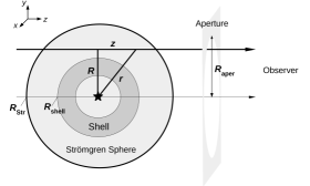
Figure 13: Schematic view of the construction of the projected surface brightness $I_{\lambda}(R)$ as a function of projected radius $R$ according to the volume emissivity $\epsilon_{\lambda}(r)$ as a function of radius $r$. The line of sight is along the $z$-axis, and the object is projected onto the $x$-$y$ plane. The object is a spherical symmetric H ii region having Strömgren radius $R_{\rm Str}$ with a spherical symmetric shell having maximum radius of $R_{\rm shell}$. The observer measures the total luminosity over a circular aperture with radius of $R_{\rm aper}$ partially (or entirely) covering the Strömgren sphere (or the shell).

The total luminosity integrated over a circular aperture entirely or partially covering a spherical symmetric H ii region (see Figure 13) with the surface brightness $I_{\lambda}(R)$ projected on the 2D plane is

$$L_{\lambda}=\int^{2\pi}_{\varphi=0}\int^{R_{\rm aper}}_{R=0}I_{\lambda}(R)RdRd\varphi,$$ (A3)

where $R_{\rm aper}$ is the radius of the circular aperture where the integral is performed over. Substituting Eq. (A1) into the above integral (A3), we restore Eq. (15).

We use Eq. (A1) to construct the 2D projected surface brightness that is comparable with the observed spatially resolved emission-line flux. Moreover, we utilize Eq. (A3) to calculate the total luminosity, which can be compared with the observed integrated emission-line flux.

To model the observed emission that is radiation bounded in the line of sight but density bounded in transverse directions, we set $R_{\rm aper}=R_{\rm shell}$ and $R_{\rm max}=R_{\rm Str}$, i.e. a partially density-bounded model, however, $R_{\rm aper}=R_{\rm max}=R_{\rm shell}$ for a fully density-bounded model, and $R_{\rm aper}=R_{\rm max}=R_{\rm Str}$ for fully radiation-bounded model, where $R_{\rm shell}$ is the outer radius of the dense shell and $R_{\rm Str}$ is the Strömgren radius (see Figure 13).

Appendix B Supplementary Material

The compressed (tar.gz) files of the interactive figure (64 images) of Figure 2, the interactive animation (64 videos) of Figure 3, and the interactive figure (192 images) of Figure 6 are available in the electronic edition of this article, and are archived on Zenodo (doi:10.5281/zenodo.4989577). These interactive figures and animation are also hosted on this URL.

The compressed (tar.gz) file containing the 6 machine-readable tables for the emission-line data (partially presented in Table 3) is available in the electronic edition of this article. Each file is named as table_case_bound.dat such as table_CPI_radi.dat, where case is for the ionization case (PI: purely photoionization and CPI: photoionization and hydrodynamic collisional ionization), and bound for the optical depth model (radi: fully radiation-bounded, pden: partially density-bounded, and dens: fully density-bounded). Each file contains the following information:

Table 3: Integrated luminosities on a logarithmic scale (unit in erg/s) from the different ionization models (see Appendix B for more information).

	radiation-bounded		part.density-bound		density-bounded
case:	PI	CPI	PI	CPI	PI	CPI
Emission Line
Ly$\alpha$ $\lambda$1216	40.836	40.577	40.443	40.191	40.317	40.077
H$\alpha$ $\lambda$6563	40.789	40.789	40.460	40.459	40.181	40.179
H$\beta$ $\lambda$4861	40.350	40.351	40.021	40.021	39.743	39.742
He i $\lambda$5876	39.435	39.440	39.112	39.112	38.834	38.833
He i $\lambda$6678	38.868	38.873	38.544	38.544	38.266	38.264
He i $\lambda$7065	39.111	39.119	38.812	38.814	38.527	38.525
He ii $\lambda$1640	38.801	38.868	38.761	38.805	38.692	38.733
He ii $\lambda$4686	37.011	37.031	37.003	37.018	36.992	37.005
C ii $\lambda$1335	38.403	38.401	37.939	37.937	37.540	37.538
C ii $\lambda$2326	38.390	38.177	37.537	37.360	35.933	35.926
C iii $\lambda$977	38.569	38.571	38.342	38.341	38.110	38.108
C iii] $\lambda$1909	39.880	39.880	39.257	39.265	38.672	38.686
C iii $\lambda$1549	36.898	36.899	36.674	36.673	36.443	36.441
C iv $\lambda$1549	39.419	39.611	39.111	39.423	38.940	39.343
[N i] $\lambda$5200	36.941	36.092	36.019	35.172	31.009	31.001
[N ii] $\lambda$5755	37.478	37.051	36.590	36.207	34.732	34.724
[N ii] $\lambda$6548	38.579	38.179	37.693	37.336	35.991	35.985
[N ii] $\lambda$6583	39.049	38.649	38.163	37.806	36.461	36.455
N iii $\lambda$1750	39.342	39.344	38.674	38.683	37.972	37.983
N iii $\lambda$991	39.056	39.059	38.816	38.816	38.578	38.576
N iv $\lambda$1486	39.152	39.210	38.770	38.861	38.470	38.620
N v $\lambda$1240	38.050	39.040	38.050	39.040	38.050	39.040
O i $\lambda$1304	38.206	38.011	37.289	37.092	33.788	33.784
[O i] $\lambda$6300	37.610	36.234	36.688	35.323	31.560	31.552
[O i] $\lambda$6364	37.114	35.739	36.193	34.827	31.064	31.056
[O ii] $\lambda$3726	38.947	38.609	38.105	37.841	36.955	36.949
[O ii] $\lambda$3729	39.093	38.753	38.248	37.980	37.055	37.049
[O ii] $\lambda$7323	37.601	37.363	36.931	36.812	36.380	36.377
[O ii] $\lambda$7332	37.518	37.280	36.846	36.726	36.290	36.288
O iii] $\lambda$1661	38.783	38.800	38.238	38.275	37.791	37.865
O iii] $\lambda$1666	39.254	39.271	38.710	38.747	38.262	38.336
[O iii] $\lambda$2321	38.542	38.552	38.061	38.076	37.676	37.697
[O iii] $\lambda$4363	39.142	39.152	38.661	38.676	38.276	38.296
[O iii] $\lambda$4959	40.564	40.568	40.162	40.164	39.834	39.834
[O iii] $\lambda$5007	41.038	41.042	40.636	40.639	40.308	40.308
…

• Table 3 is published in its entirety in the machine-readable format. A portion is shown here for guidance regarding its form and content.

• Parameters in the example model are as follows: metallicity $Z/$Z${}_{\odot}=0.5$, mass-loss rate $\dot{M}_{\rm sc}=0.607\times 10^{-2}$ M_⊙ yr^-1, wind terminal speed $V_{\infty}=457$ km s^-1, cluster radius $R_{\rm sc}=1$ pc, total stellar mass $M_{\star}=2.05\times 10^{6}$ M_⊙, age $t=1$ Myr, ambient density $n_{\rm amb}=100$ cm^-3, and ambient temperature $T_{\rm amb}$ calculated by cloudy.

• metal: metallicity $\hat{Z}\equiv Z/$Z${}_{\odot}=1$, $0.5$, $0.25$, and $0.125$.

• dMdt: mass-loss rate $\dot{M}_{\rm sc}=10^{-1}$, $10^{-2}$, $10^{-3}$, and $10^{-4}\times\hat{Z}^{0.72}$ M_⊙ yr^-1.

• Vinf: wind terminal speed $V_{\infty}=250$, $500$, and $1000\times\hat{Z}^{0.13}$ km s^-1.

• Rsc: cluster radius $R_{\rm sc}=1$ pc.

• age: current age $t=1$ Myr.

• Mstar: total stellar mass $M_{\star}=2.05\times 10^{6}$ M_⊙.

• logLion: ionizing luminosity $\log L_{\rm ion}$ (erg/s).

• Namb: ambient density $n_{\rm amb}=1$, 10, $10^{2}$, and $10^{3}$ cm^-3.

• Tamb: mean ambient temperature $T_{\rm amb}$ determined by cloudy.

• Rmax: maximum radius $R_{\rm max}$ (pc) for the surface brightness integration.

• Raper: aperture radius $R_{\rm aper}$ (pc) for the total luminosity integration.

• Rshell: shell outer radius $R_{\rm shell}$ (pc).

• Rstr: Strömgren radius $R_{\rm str}$ (pc) determined by cloudy.

• Rbin: bubble inner radius $R_{\rm b,in}$ (pc).

• Rbout: bubble outer radius $R_{\rm b,out}$ (pc) or shell inner radius.

• Tbubble: median temperature $T_{\rm bubble}$ of the hot bubble (region b in Figure 2).

• Tadi: median temperature $T_{\rm adi,med}$ of the expanding wind predicted by the adiabatic solutions (region a in Figure 2).

• Twind: median temperature $T_{\rm w,med}$ of the expanding wind calculated by maihem with the radiative solutions (region a in Figure 2).

• logUsp: dimensionless ionization parameter $\log U_{\rm sph}$ in a spherical geometry calculated by cloudy, defined as $U_{\rm sph}\equiv Q({\rm H}^{0})/4\pi R^{2}_{\rm str}n_{\rm H}c$, where $Q({\rm H}^{0})$ is the total number of hydrogen-ionizing photons emitted per second, $n_{\rm H}$ the hydrogen density, and $c$ the speed of light.

• thin: optically thin (1) or thick (0) model.

• mode: the cooling/heating radiative/adiabatic modes: 1 (AW: adiabatic wind), 2 (AB: adiabatic bubble), 3 (AP: adiabatic, pressure-confined), 4 (CC: catastrophic cooling), 5 (CB: catastrophic cooling bubble), and 6 (CP: catastrophic cooling, pressure-confined).

• H_1_1216, H_1_6563, …, Ar_5_7006: integrated luminosities of the emission lines Ly$\alpha$ $\lambda$1216 Å, H$\alpha$ $\lambda$6563 Å, …, [Ar v] $\lambda$7006 Å, respectively.

ORCID iDs

Ashkbiz Danehkar https://orcid.org/0000-0003-4552-5997

M. S. Oey https://orcid.org/0000-0002-5808-1320

William J. Gray https://orcid.org/0000-0001-9014-3125

References

- Añorve-Zeferino et al. (2009) Añorve-Zeferino, G. A., Tenorio-Tagle, G., & Silich, S. 2009, MNRAS, 394, 1284
- Abbott (1982) Abbott, D. C. 1982, ApJ, 263, 723
- Abbott et al. (1981) Abbott, D. C., Bieging, J. H., & Churchwell, E. 1981, ApJ, 250, 645
- Allen et al. (1998) Allen, M. G., Dopita, M. A., & Tsvetanov, Z. I. 1998, ApJ, 493, 571
- Amorín et al. (2017) Amorín, R., Fontana, A., Pérez-Montero, E., et al. 2017, Nature Astron., 1, 0052
- Badnell (2006) Badnell, N. R. 2006, ApJS, 167, 334
- Baldwin et al. (2003) Baldwin, J. A., Hamann, F., Korista, K. T., et al. 2003, ApJ, 583, 649
- Baldwin et al. (1981) Baldwin, J. A., Phillips, M. M., & Terlevich, R. 1981, PASP, 93, 5
- Berg et al. (2016) Berg, D. A., Skillman, E. D., Henry, R. B. C., Erb, D. K., & Carigi, L. 2016, ApJ, 827, 126
- Bielby et al. (2019) Bielby, R. M., Stott, J. P., Cullen, F., et al. 2019, MNRAS, 486, 21
- Bruhweiler et al. (1980) Bruhweiler, F. C., Gull, T. R., Kafatos, M., & Sofia, S. 1980, ApJ, 238, L27
- Cantó et al. (2000) Cantó, J., Raga, A. C., & Rodríguez, L. F. 2000, ApJ, 536, 896
- Cardamone et al. (2009) Cardamone, C., Schawinski, K., Sarzi, M., et al. 2009, MNRAS, 399, 1191
- Cash et al. (1980) Cash, W., Charles, P., Bowyer, S., et al. 1980, ApJ, 238, L71
- Castor et al. (1975) Castor, J., McCray, R., & Weaver, R. 1975, ApJ, 200, L107
- Cavaliere (1980) Cavaliere, A. 1980, X-Ray Astronomy, ed. R. Giacconi & G. Setti (Dordrecht: Springer Netherlands), 217–237
- Chevalier & Clegg (1985) Chevalier, R. A. & Clegg, A. W. 1985, Nature, 317, 44, (CC85)
- Chisholm et al. (2018) Chisholm, J., Bordoloi, R., Rigby, J. R., & Bayliss, M. 2018, MNRAS, 474, 1688
- Chu et al. (1995) Chu, Y.-H., Chang, H.-W., Su, Y.-L., & Mac Low, M.-M. 1995, ApJ, 450, 157
- Chu & Mac Low (1990) Chu, Y.-H. & Mac Low, M.-M. 1990, ApJ, 365, 510
- Cimatti et al. (2019) Cimatti, A., Fraternali, F., & Nipoti, C. 2019, Introduction to Galaxy Formation and Evolution: From Primordial Gas to Present-Day Galaxies (Cambridge University Press)
- Creasey et al. (2013) Creasey, P., Theuns, T., & Bower, R. G. 2013, MNRAS, 429, 1922
- Dahlem (1997) Dahlem, M. 1997, PASP, 109, 1298
- Dahlem et al. (1997) Dahlem, M., Petr, M. G., Lehnert, M. D., Heckman, T. M., & Ehle, M. 1997, A&A, 320, 731
- de Barros et al. (2016) de Barros, S., Vanzella, E., Amorín, R., et al. 2016, A&A, 585, A51
- De Vis et al. (2019) De Vis, P., Jones, A., Viaene, S., et al. 2019, A&A, 623, A5
- Dove et al. (2000) Dove, J. B., Shull, J. M., & Ferrara, A. 2000, ApJ, 531, 846
- Edmunds (2001) Edmunds, M. G. 2001, MNRAS, 328, 223
- Einfeldt (1988) Einfeldt, B. 1988, SIAM J. Numer. Anal., 25, 294
- Einfeldt et al. (1991) Einfeldt, B., Roe, P. L., Munz, C. D., & Sjogreen, B. 1991, J. Comput. Phys., 92, 273
- Ekström et al. (2012) Ekström, S., Georgy, C., Eggenberger, P., et al. 2012, A&A, 537, A146
- Fabbiano (1988) Fabbiano, G. 1988, ApJ, 330, 672
- Falgout & Yang (2002) Falgout, R. D. & Yang, U. M. 2002, in Computational Science – ICCS 2002. Lecture Notes in Computer Science, ed. P. Sloot, A. Hoekstra, C. Tan, & J. Dongarra, Vol. 2331 (Berlin, Heidelberg: Springer), 632–641
- Feltre et al. (2016) Feltre, A., Charlot, S., & Gutkin, J. 2016, MNRAS, 456, 3354
- Ferland et al. (2017) Ferland, G. J., Chatzikos, M., Guzmán, F., et al. 2017, RMxAA, 53, 385
- Ferland et al. (1998) Ferland, G. J., Korista, K. T., Verner, D. A., et al. 1998, PASP, 110, 761
- Ferland et al. (2013) Ferland, G. J., Porter, R. L., van Hoof, P. A. M., et al. 2013, RMxAA, 49, 137
- Ferrara et al. (2000) Ferrara, A., Pettini, M., & Shchekinov, Y. 2000, MNRAS, 319, 539
- Folk et al. (2011) Folk, M., Heber, G., Koziol, Q., Pourmal, E., & Robinson, D. 2011, in Proc. EDBT/ICDT 2011 Workshop on Array Databases (New York, NY: ACM), 36–47
- Fryxell et al. (2000) Fryxell, B., Olson, K., Ricker, P., et al. 2000, ApJS, 131, 273
- Fujimoto et al. (2019) Fujimoto, S., Ouchi, M., Ferrara, A., et al. 2019, ApJ, 887, 107
- Fujimoto et al. (2020) Fujimoto, S., Silverman, J. D., Bethermin, M., et al. 2020, ApJ, 900, 1
- Galliano et al. (2008) Galliano, E., Alloin, D., Pantin, E., et al. 2008, A&A, 492, 3
- Garnett et al. (1999) Garnett, D. R., Shields, G. A., Peimbert, M., et al. 1999, ApJ, 513, 168
- Garnett et al. (1995) Garnett, D. R., Skillman, E. D., Dufour, R. J., et al. 1995, ApJ, 443, 64
- Georgy et al. (2013) Georgy, C., Ekström, S., Eggenberger, P., et al. 2013, A&A, 558, A103
- Georgy et al. (2012) Georgy, C., Ekström, S., Meynet, G., et al. 2012, A&A, 542, A29
- Gilbert & Graham (2007) Gilbert, A. M. & Graham, J. R. 2007, ApJ, 668, 168
- Gnat & Ferland (2012) Gnat, O. & Ferland, G. J. 2012, ApJS, 199, 20
- Gnedin & Hollon (2012) Gnedin, N. Y. & Hollon, N. 2012, ApJS, 202, 13
- Gray et al. (2019a) Gray, W. J., Oey, M. S., Silich, S., & Scannapieco, E. 2019a, ApJ, 887, 161, (Paper I)
- Gray & Scannapieco (2016) Gray, W. J. & Scannapieco, E. 2016, ApJ, 818, 198
- Gray et al. (2015) Gray, W. J., Scannapieco, E., & Kasen, D. 2015, ApJ, 801, 107
- Gray et al. (2019b) Gray, W. J., Scannapieco, E., & Lehnert, M. D. 2019b, ApJ, 875, 110
- Grazian et al. (2015) Grazian, A., Fontana, A., Santini, P., et al. 2015, A&A, 575, A96
- Groves et al. (2004) Groves, B. A., Dopita, M. A., & Sutherland, R. S. 2004, ApJS, 153, 75
- Groves et al. (2006) Groves, B. A., Heckman, T. M., & Kauffmann, G. 2006, MNRAS, 371, 1559
- Gutkin et al. (2016) Gutkin, J., Charlot, S., & Bruzual, G. 2016, MNRAS, 462, 1757
- Hainline et al. (2011) Hainline, K. N., Shapley, A. E., Greene, J. E., & Steidel, C. C. 2011, ApJ, 733, 31
- Harris et al. (2020) Harris, C. R., Millman, K. J., van der Walt, S. J., et al. 2020, Nature, 585, 357
- Hayes et al. (2016) Hayes, M., Melinder, J., Östlin, G., et al. 2016, ApJ, 828, 49
- Heckman (2002) Heckman, T. M. 2002, ASP Conf. Ser., Vol. 254, Galactic Superwinds Circa 2001, ed. J. S. Mulchaey & J. T. Stocke, 292
- Heckman et al. (1987) Heckman, T. M., Armus, L., & Miley, G. K. 1987, AJ, 93, 276
- Heckman et al. (1990) Heckman, T. M., Armus, L., & Miley, G. K. 1990, ApJS, 74, 833
- Heckman et al. (1995) Heckman, T. M., Dahlem, M., Lehnert, M. D., et al. 1995, ApJ, 448, 98
- Heckman et al. (1993) Heckman, T. M., Lehnert, M. D., & Armus, L. 1993, in The Environment and Evolution of Galaxies, Astrophysics and Space Science Library, Vol. 188, Galactic Superwinds, ed. J. M. Shull & H. A. Thronson (Springer, Dordrecht), 455
- Heckman et al. (2001) Heckman, T. M., Sembach, K. R., Meurer, G. R., et al. 2001, ApJ, 554, 1021
- Hillier & Miller (1998) Hillier, D. J. & Miller, D. L. 1998, ApJ, 496, 407
- Hirashita (1999) Hirashita, H. 1999, ApJ, 522, 220
- Hirschmann et al. (2019) Hirschmann, M., Charlot, S., Feltre, A., et al. 2019, MNRAS, 487, 333
- Holtzman et al. (1992) Holtzman, J. A., Faber, S. M., Shaya, E. J., et al. 1992, AJ, 103, 691
- Hopkins et al. (2012) Hopkins, P. F., Quataert, E., & Murray, N. 2012, MNRAS, 421, 3522
- Hunter (2007) Hunter, J. D. 2007, Comput. Sci. Eng., 9, 90
- Izotov et al. (2016) Izotov, Y. I., Orlitová, I., Schaerer, D., et al. 2016, Nature, 529, 178
- Izotov et al. (2018) Izotov, Y. I., Schaerer, D., Worseck, G., et al. 2018, MNRAS, 474, 4514
- Jaskot et al. (2019) Jaskot, A. E., Dowd, T., Oey, M. S., Scarlata, C., & McKinney, J. 2019, ApJ, 885, 96
- Jaskot et al. (2017) Jaskot, A. E., Oey, M. S., Scarlata, C., & Dowd, T. 2017, ApJ, 851, L9
- Kauffmann et al. (2003) Kauffmann, G., Heckman, T. M., Tremonti, C., et al. 2003, MNRAS, 346, 1055
- Keenan et al. (2017) Keenan, R. P., Oey, M. S., Jaskot, A. E., & James, B. L. 2017, ApJ, 848, 12
- Kewley et al. (2013) Kewley, L. J., Dopita, M. A., Leitherer, C., et al. 2013, ApJ, 774, 100
- Kewley et al. (2001) Kewley, L. J., Dopita, M. A., Sutherland, R. S., Heisler, C. A., & Trevena, J. 2001, ApJ, 556, 121
- Kewley et al. (2006) Kewley, L. J., Groves, B., Kauffmann, G., & Heckman, T. 2006, MNRAS, 372, 961
- Koo & McKee (1992a) Koo, B.-C. & McKee, C. F. 1992a, ApJ, 388, 93
- Koo & McKee (1992b) Koo, B.-C. & McKee, C. F. 1992b, ApJ, 388, 103
- Lee (2013) Lee, D. 2013, J. Comput. Phys., 243, 269
- Lee & Deane (2009) Lee, D. & Deane, A. E. 2009, J. Comput. Phys., 228, 952
- Lee et al. (2009) Lee, D., Deane, A. E., & Federrath, C. 2009, ASP Conf. Ser., Vol. 406, A New Multidimensional Unsplit MHD Solver in FLASH3, ed. N. V. Pogorelov, E. Audit, P. Colella, & G. P. Zank, 243
- Lehnert & Heckman (1995) Lehnert, M. D. & Heckman, T. M. 1995, ApJS, 97, 89
- Lehnert & Heckman (1996) Lehnert, M. D. & Heckman, T. M. 1996, ApJ, 462, 651
- Leitherer et al. (2014) Leitherer, C., Ekström, S., Meynet, G., et al. 2014, ApJS, 212, 14
- Leitherer et al. (1992) Leitherer, C., Robert, C., & Drissen, L. 1992, ApJ, 401, 596
- Leitherer et al. (1999) Leitherer, C., Schaerer, D., Goldader, J. D., et al. 1999, ApJS, 123, 3
- Levesque et al. (2012) Levesque, E. M., Leitherer, C., Ekstrom, S., Meynet, G., & Schaerer, D. 2012, ApJ, 751, 67
- Lloyd-Davies et al. (2000) Lloyd-Davies, E. J., Ponman, T. J., & Cannon, D. B. 2000, MNRAS, 315, 689
- Lochhaas et al. (2018) Lochhaas, C., Thompson, T. A., Quataert, E., & Weinberg, D. H. 2018, MNRAS, 481, 1873
- Löhner (1987) Löhner, R. 1987, Comp. Meth. Appl. Mech. Eng., 61, 323
- Longair (2008) Longair, M. 2008, Galaxy Formation, Astronomy and Astrophysics Library (Springer Berlin Heidelberg)
- Mac Low & Ferrara (1999) Mac Low, M.-M. & Ferrara, A. 1999, ApJ, 513, 142
- Mac Low & McCray (1988) Mac Low, M.-M. & McCray, R. 1988, ApJ, 324, 776
- MacNeice et al. (2000) MacNeice, P., Olson, K. M., Mobarry, C., de Fainchtein, R., & Packer, C. 2000, Comput. Phys. Comm., 126, 330
- Maeder (1990) Maeder, A. 1990, A&AS, 84, 139
- Magnier et al. (1996) Magnier, E. A., Chu, Y.-H., Points, S. D., Hwang, U., & Smith, R. C. 1996, ApJ, 464, 829
- Marlowe et al. (1995) Marlowe, A. T., Heckman, T. M., Wyse, R. F. G., & Schommer, R. 1995, ApJ, 438, 563
- Martin (2005) Martin, C. L. 2005, ApJ, 621, 227
- Martins et al. (2005) Martins, L. P., González Delgado, R. M., Leitherer, C., Cerviño, M., & Hauschildt, P. 2005, MNRAS, 358, 49
- Masters et al. (2014) Masters, D., McCarthy, P., Siana, B., et al. 2014, ApJ, 785, 153
- McCarthy et al. (1987) McCarthy, P. J., van Breugel, W., & Heckman, T. 1987, AJ, 93, 264
- McDonald et al. (2015) McDonald, M., McNamara, B. R., van Weeren, R. J., et al. 2015, ApJ, 811, 111
- Melo et al. (2005) Melo, V. P., Muñoz-Tuñón, C., Maíz-Apellániz, J., & Tenorio-Tagle, G. 2005, ApJ, 619, 270
- Meyer et al. (1998) Meyer, D. M., Jura, M., & Cardelli, J. A. 1998, ApJ, 493, 222
- Micheva et al. (2020) Micheva, G., Östlin, G., Melinder, J., et al. 2020, ApJ, 903, 123
- Mokiem et al. (2007) Mokiem, M. R., de Koter, A., Vink, J. S., et al. 2007, A&A, 473, 603
- Nakajima & Ouchi (2014) Nakajima, K. & Ouchi, M. 2014, MNRAS, 442, 900
- Nath & Trentham (1997) Nath, B. B. & Trentham, N. 1997, MNRAS, 291, 505
- Norman & Ikeuchi (1989) Norman, C. A. & Ikeuchi, S. 1989, ApJ, 345, 372
- Nozawa et al. (2010) Nozawa, T., Kozasa, T., Tominaga, N., et al. 2010, ApJ, 713, 356
- O’Connell et al. (1995) O’Connell, R. W., Gallagher, John S., I., Hunter, D. A., & Colley, W. N. 1995, ApJ, 446, L1
- Oey et al. (2017) Oey, M. S., Herrera, C. N., Silich, S., et al. 2017, ApJ, 849, L1
- Oey & Massey (1995) Oey, M. S. & Massey, P. 1995, ApJ, 452, 210
- Oppenheimer & Schaye (2013) Oppenheimer, B. D. & Schaye, J. 2013, MNRAS, 434, 1043
- Osterbrock et al. (1992) Osterbrock, D. E., Tran, H. D., & Veilleux, S. 1992, ApJ, 389, 196
- Ostriker & McKee (1988) Ostriker, J. P. & McKee, C. F. 1988, Rev. Mod. Phys., 60, 1
- Patnaude et al. (2009) Patnaude, D. J., Ellison, D. C., & Slane, P. 2009, ApJ, 696, 1956
- Patnaude et al. (2010) Patnaude, D. J., Slane, P., Raymond, J. C., & Ellison, D. C. 2010, ApJ, 725, 1476
- Patrício et al. (2016) Patrício, V., Richard, J., Verhamme, A., et al. 2016, MNRAS, 456, 4191
- Pauldrach et al. (2001) Pauldrach, A. W. A., Hoffmann, T. L., & Lennon, M. 2001, A&A, 375, 161
- Pettini et al. (2002) Pettini, M., Rix, S. A., Steidel, C. C., et al. 2002, ApJ, 569, 742
- Pettini et al. (2001) Pettini, M., Shapley, A. E., Steidel, C. C., et al. 2001, ApJ, 554, 981
- Pizzati et al. (2020) Pizzati, E., Ferrara, A., Pallottini, A., et al. 2020, MNRAS, 495, 160
- Raymond et al. (1976) Raymond, J. C., Cox, D. P., & Smith, B. W. 1976, ApJ, 204, 290
- Reynolds et al. (2001) Reynolds, R. J., Sterling, N. C., & Haffner, L. M. 2001, ApJ, 558, L101
- Richard et al. (2011) Richard, J., Jones, T., Ellis, R., et al. 2011, MNRAS, 413, 643
- Richings et al. (2014) Richings, A. J., Schaye, J., & Oppenheimer, B. D. 2014, MNRAS, 440, 3349
- Roe (1981) Roe, P. L. 1981, J. Comput. Phys., 43, 357
- Rupke et al. (2002) Rupke, D. S., Veilleux, S., & Sanders, D. B. 2002, ApJ, 570, 588
- Rupke et al. (2005) Rupke, D. S., Veilleux, S., & Sanders, D. B. 2005, ApJS, 160, 115
- Sakamoto et al. (2006) Sakamoto, K., Ho, P. T. P., Iono, D., et al. 2006, ApJ, 636, 685
- Salpeter (1955) Salpeter, E. E. 1955, ApJ, 121, 161
- Sarazin (1986) Sarazin, C. L. 1986, Rev. Mod. Phys., 58, 1
- Satyapal et al. (1997) Satyapal, S., Watson, D. M., Pipher, J. L., et al. 1997, ApJ, 483, 148
- Savage et al. (1977) Savage, B. D., Bohlin, R. C., Drake, J. F., & Budich, W. 1977, ApJ, 216, 291
- Savage et al. (2014) Savage, B. D., Kim, T. S., Wakker, B. P., et al. 2014, ApJS, 212, 8
- Saxena et al. (2020) Saxena, A., Pentericci, L., Mirabelli, M., et al. 2020, A&A, 636, A47
- Scannapieco et al. (2002) Scannapieco, E., Ferrara, A., & Madau, P. 2002, ApJ, 574, 590
- Senchyna et al. (2017) Senchyna, P., Stark, D. P., Vidal-García, A., et al. 2017, MNRAS, 472, 2608
- Shibuya et al. (2015) Shibuya, T., Ouchi, M., & Harikane, Y. 2015, ApJS, 219, 15
- Silich & Tenorio-Tagle (2018) Silich, S. & Tenorio-Tagle, G. 2018, MNRAS, 478, 5112
- Silich et al. (2005) Silich, S., Tenorio-Tagle, G., & Añorve-Zeferino, G. A. 2005, ApJ, 635, 1116
- Silich et al. (2020) Silich, S., Tenorio-Tagle, G., Martínez-González, S., & Turner, J. 2020, MNRAS, 494, 97
- Silich et al. (2003) Silich, S., Tenorio-Tagle, G., & Muñoz-Tuñón, C. 2003, ApJ, 590, 791
- Silich et al. (2007) Silich, S., Tenorio-Tagle, G., & Muñoz-Tuñón, C. 2007, ApJ, 669, 952
- Silich et al. (2004) Silich, S., Tenorio-Tagle, G., & Rodríguez-González, A. 2004, ApJ, 610, 226
- Smith et al. (2006) Smith, L. J., Westmoquette, M. S., Gallagher, J. S., et al. 2006, MNRAS, 370, 513
- Stark et al. (2014) Stark, D. P., Richard, J., Siana, B., et al. 2014, MNRAS, 445, 3200
- Stark et al. (2015) Stark, D. P., Walth, G., Charlot, S., et al. 2015, MNRAS, 454, 1393
- Steidel et al. (2010) Steidel, C. C., Erb, D. K., Shapley, A. E., et al. 2010, ApJ, 717, 289
- Steidel et al. (2016) Steidel, C. C., Strom, A. L., Pettini, M., et al. 2016, ApJ, 826, 159
- Strickland et al. (2002) Strickland, D. K., Heckman, T. M., Weaver, K. A., Hoopes, C. G., & Dahlem, M. 2002, ApJ, 568, 689
- Strickland & Stevens (1999) Strickland, D. K. & Stevens, I. R. 1999, MNRAS, 306, 43
- Tasca et al. (2015) Tasca, L. A. M., Le Fèvre, O., Hathi, N. P., et al. 2015, A&A, 581, A54
- Tenorio-Tagle et al. (2005) Tenorio-Tagle, G., Silich, S., Rodríguez-González, A., & Muñoz-Tuñón, C. 2005, ApJ, 620, 217
- Tenorio-Tagle et al. (2007) Tenorio-Tagle, G., Wünsch, R., Silich, S., & Palouš, J. 2007, ApJ, 658, 1196
- Thornton et al. (1998) Thornton, K., Gaudlitz, M., Janka, H. T., & Steinmetz, M. 1998, ApJ, 500, 95
- Toro et al. (1994) Toro, E. F., Spruce, M., & Speares, W. 1994, Shock Waves, 4, 25
- Tripp et al. (2008) Tripp, T. M., Sembach, K. R., Bowen, D. V., et al. 2008, ApJS, 177, 39
- Tsai et al. (2009) Tsai, A.-L., Matsushita, S., Nakanishi, K., et al. 2009, PASJ, 61, 237
- Turk et al. (2011) Turk, M. J., Smith, B. D., Oishi, J. S., et al. 2011, ApJS, 192, 9
- Turner et al. (2003) Turner, J. L., Beck, S. C., Crosthwaite, L. P., et al. 2003, Nature, 423, 621
- Turner et al. (2017) Turner, J. L., Consiglio, S. M., Beck, S. C., et al. 2017, ApJ, 846, 73
- van Leer (1979) van Leer, B. 1979, J. Comput. Phys., 32, 101
- Vanzella et al. (2016) Vanzella, E., De Barros, S., Cupani, G., et al. 2016, ApJ, 821, L27
- Vázquez & Leitherer (2005) Vázquez, G. A. & Leitherer, C. 2005, ApJ, 621, 695
- Veilleux et al. (2005) Veilleux, S., Cecil, G., & Bland-Hawthorn, J. 2005, ARA&A, 43, 769
- Veilleux et al. (1994) Veilleux, S., Cecil, G., Bland-Hawthorn, J., et al. 1994, ApJ, 433, 48
- Veilleux & Osterbrock (1987) Veilleux, S. & Osterbrock, D. E. 1987, ApJS, 63, 295
- Verner et al. (1996) Verner, D. A., Ferland, G. J., Korista, K. T., & Yakovlev, D. G. 1996, ApJ, 465, 487
- Verner & Yakovlev (1995) Verner, D. A. & Yakovlev, D. G. 1995, A&AS, 109, 125
- Vink et al. (2001) Vink, J. S., de Koter, A., & Lamers, H. J. G. L. M. 2001, A&A, 369, 574
- Virtanen et al. (2020) Virtanen, P., Gommers, R., Oliphant, T. E., et al. 2020, Nature Methods, 17, 261
- Voronov (1997) Voronov, G. S. 1997, Atom. Data Nucl. Data Tabl., 65, 1
- Weaver et al. (1977) Weaver, R., McCray, R., Castor, J., Shapiro, P., & Moore, R. 1977, ApJ, 218, 377
- Weiß et al. (1999) Weiß, A., Walter, F., Neininger, N., & Klein, U. 1999, A&A, 345, L23
- Westmoquette et al. (2014) Westmoquette, M. S., Bastian, N., Smith, L. J., et al. 2014, ApJ, 789, 94
- Wilman et al. (2005) Wilman, R. J., Gerssen, J., Bower, R. G., et al. 2005, Nature, 436, 227
- Wolfire et al. (2003) Wolfire, M. G., McKee, C. F., Hollenbach, D., & Tielens, A. G. G. M. 2003, ApJ, 587, 278
- Zhang et al. (2019) Zhang, G.-Y., Slavin, J. D., Foster, A., et al. 2019, ApJ, 875, 81