The peak-and-end rule and differential equations with maxima: a view on the unpredictability of happiness

Abstract

In the 1990s, after a series of experiments, the behavioral psychologist and economist Daniel Kahneman and his colleagues formulated the following Peak-End evaluation rule: the remembered utility of pleasant or unpleasant episodes is accurately predicted by averaging the Peak (most intense value) of instant utility (or disutility) recorded during an episode and the instant utility recorded near the end of the experience (D. Kahneman et al., 1997, QJE, p. 381). Hence, the simplest mathematical model for time evolution of the experienced utility function $u=u(t)$ can be given by the scalar differential equation $u^{\prime}(t)=au(t)+b\max\{u(s):s\in[t-h,t]\}+f(t)\ (*),$ where $f$ represents exogenous stimuli, $h$ is the maximal duration of the experience, and $a,b\in{\mathbb{R}}$ are some averaging weights. In this work, we study equation $(*)$ and show that, for a range of parameters $a,b,h$ and a periodic sine-like term $f$, the dynamics of $(*)$ can be completely described in terms of an associated one-dimensional dynamical system generated by a piece-wise continuous map from a finite interval into itself. We illustrate our approach with two examples. In particular, we show that the hedonic utility $u(t)$ (‘happiness’) can exhibit chaotic behavior.

To the memory of Anatoly Samoilenko (1938-2020)

1 Introduction

In the 1990s, after a series of experiments, the behavioral psychologist (and Nobel laureate in economics) Daniel Kahneman with his colleagues formulated the following Peak-End evaluation rule: the remembered utility of pleasant or unpleasant episodes is accurately predicted by averaging the Peak (most intense value) of instant utility (or disutility) recorded during an episode and the instant utility recorded near the end of the experience (excerpt from [19], p. 381). This rule obtained multiple applications (including customer service, price setting strategies, medical procedures, education etc) and nowadays, the Peak-End theory has become one of the active areas of research in the field of behavioral science, e.g. see [5, 18, 19, 20, 28, 40] and references therein.

Accordingly, the simplest mathematical model for time evolution of the experienced utility function $u=u(t)$ can be given by the scalar differential equation

$$u^{\prime}(t)=au(t)+b\max\limits_{s\in[t-h,t]}u(s)+f(t)$$ (1)

where $f$ represents exogenous stimuli, $h>0$ is the maximal duration of the experience and $a,b$ are some real coefficients. The determination of qualitatively plausible psychological parameters $f,a,b$ seems to be a rather difficult task (which we do not address here); on the other hand, it is reasonable to consider the case when $f$ is a $T$-periodic continuous sine-like function (see Definition 1 below), assuming that the rate of change of the utility $u(t)$ is affected by linear decay (with coefficient $\alpha>0$) and is proportional (with coefficient $\beta>0$) to the difference between its instant value and its peak on the precedent fixed time interval:

$$u^{\prime}(t)=-\alpha u(t)+\beta(u(t)-\max\limits_{s\in[t-h,t]}u(s))+f(t).$$ (2)

Akin evolutionary rules, with the term $u(t-h)$ instead of $\max\{u(s):s\in[t-h,t]\}$, can be found in other comparable cases: see, for instance, the celebrated Kalecki difference-differential equation describing a macroeconomic model of business cycles [9, 21, 23] or the mathematical model of emotional balance dynamics proposed in [36]. The works [4, 7] show how the psychology of agents trading the foreign currency generates a similar dynamical mechanism expressed by the equation

$$u^{\prime}(t)=-b|u(t)|u(t)+a(u(t)-u(t-1)),\quad a,b>0.$$

Comparing equations (1) and (2), we obtain that $a=\beta-\alpha,\ b=-\beta$. In this way, the situation when $b<0$ and $a+b<0$ might appear as more interesting from the applied point of view, and, as we manifest in the present paper, it is certainly more interesting by its mathematical implications. In particular, we will show that for a range of parameters $a,b,h$ and a periodic term $f$, the dynamics of (1) can exhibit chaotic behavior.

Even assuming that equation (2) is a phenomenological model, our study could be considered as another attempt to use mathematics to understand the behaviour of happiness, a topic that goes back at least to Edgeworth’s calculus of pleasure or “hedonimetry” in 1881 [6]. Indeed, ‘Happiness’ [12] is one of the possible interpretations of the experienced utility, and, from their own individual experience, everyone knows that happiness is unpredictable [11]. Remarkably, there exist well-documented descriptions of visibly chaotic time evolution of happiness [17], see Figure 1 and compare it with a numerical solution obtained for a particular case of (1) in Figure 5.

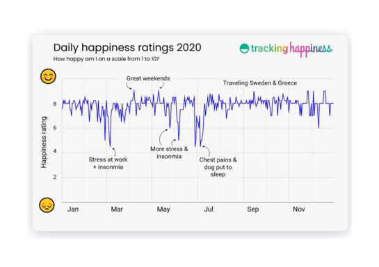
Figure 1: The 2020 Happiness review by H. Huijer taken from [17]. The figure is published with the kind permission of Hugo Huijer.

In any event, the main goal of our studies is the elaboration of a satisfactory mathematical framework to deal with the quasilinear functional differential equation (1). As far as we know, the first article dedicated to equations with maxima appeared in 1964 [31] and in the survey [29, Section 12] on the theory of functional differential equations, A. Myshkis singled out systems with maxima as differential equations with deviating argument of complex structure. Particularly he noted that ‘the specific character of these questions is not yet sufficiently clear’ [29, p. 199]. Denote by $C[-h,0]$ the set of continuous functions from $[-h,0]$ to ${\mathbb{R}}$. We notice that the functional $f:{\mathbb{R}}\times C[-h,0]\to{\mathbb{R}}$ defined by $f(t,\phi)=a\phi(0)+b\max\{\phi(s):s\in[-h,0]\}+f(t)$, which corresponds to the right-hand side of (1), is globally Lipshitzian in $\phi$, which guarantees the existence, uniqueness, global continuation and continuous dependence on initial data of the solutions to (1). However, this functional is not differentiable in $\phi$. By using the representation $\max\{\phi(s),s\in[-h,0]\}=\phi(-\tau(\phi))$ for some $\tau(\phi)\in[0,h]$, we see that (1) can be considered as a functional differential equation with state-dependent delay. Note that function $\tau:C[-h,0]\to[0,h]$ is clearly discontinuous at each constant element. The above considerations show that an appropriate functional space for the evolutionary system (1) should be the space of continuously differentiable functions $C^{1}[-h,0]$ instead of $C[-h,0]$, cf. [32].

We will call (1) the Magomedov equation, in honor of the Azerbaijani mathematician who introduced this model in the late 70s and since then has analyzed several particular cases of it with periodic forcing term $f(t)$, see [1, 3, 27, 34, 35]. In his monograph [27] dedicated to equations with maxima, Magomedov explains how the periodic equation (1) can be used for modeling automatic control of voltage in a generator of constant current, see [27, pp. 4–7].

Besides the above mentioned applications, the periodic equation (1) plays an important role in the stability theory for the delay differential equation

$$u^{\prime}(t)=au(t)+bf(t,u_{t}),$$

where $a,b<0$, $u_{t}(s)=u(t+s),\ s\in[-h,0]$, and the continuous functional $f:{\mathbb{R}}\times C[-h,0]\to{\mathbb{R}}$ satisfies either the following (sublinear) Yorke condition [39]

$$-\max_{s\in[-h,0]}(-\phi(s))\leq f(t,\phi)\leq\max_{s\in[-h,0]}\phi(s),\ t\geq 0,\ \phi\in C[-h,0],$$ (3)

or its generalized (nonlinear) version introduced in [25]. In this context, model (1) is used as a key test equation whose analysis determines the optimal stability regions for equations satisfying one of the aforementioned Yorke conditions. For instance, in the simplest situation when $a=0$, equation (1) has a uniformly asymptotically stable periodic solution for every periodic function $f(t)$ if and only if $0<-bh<3/2$ (that constitutes a variant of the so-called Myshkis-Wright-Yorke 3/2-stability criterion, see [8, 24, 26, 32]).

Among other mathematical objects closely related to equation (1), we would like to mention the Hausrath equation

$$u^{\prime}(t)=b(\max_{s\in[t-h,t]}|u(s)|-u(t)),$$

analyzed in [16, pp. 73-74] and the Halanay inequality

$$u^{\prime}(t)\leq au(t)+b\max_{s\in[t-h,t]}u(s)$$

which became an important tool in the stability theory of functional differential equations, see [2, 3, 10, 13] for the further references.

The present work extends previous studies [3, 32] where, in particular, the existence of multiple periodic solutions to equation (1) was established by using Krasnoselsky’s rotation number and introducing a substitute of the variational equation for the non-smooth model (1). Our approach in this paper is cardinally different, its workhorse is an associated selfmap $\cal R$ of an interval called ‘the return map’ in the paper. This function allows us to reproduce the sequence of consecutive ‘qualified’ local maxima $q_{j}>q$ (i.e. having the property $u(q_{j},p)=\max_{s\in[q_{j}-h,q_{j}]}u(s,p)$) of each solution $u(t,p)$ to (1) with initial condition $u(s,p)=p,$ $s\in[q-h,q]$ (actually, we will define $\cal R$ by ${\cal R}(p)=u(q_{1},p)$). As we will show, the information stored in $\cal R$ is well enough to describe the dynamics in (1). Now, analysing the dependence of the ‘qualified’ local maximum $u(q_{1},p)$ on $p$, one can observe that at some specific values of $p$ this maximum disappears due to a cusp catastrophe. Accordingly, the return map $\cal R$ has a discontinuity at each such point so that important efforts in Section 2 are focused on the studies of the continuity and differentiability properties of $\cal R$. In particular, while computing the derivative ${\cal R}^{\prime}(p)$, we have found another interpretation of the aforementioned variational equation for (1).

Finally, in Section 3 we show that, in spite of the uniqueness of $T$-periodic solution to (1) for all sufficiently small and large values of $hT^{-1}$, in general equation (1) possesses a global attractor ${\cal A}$ with rather complicated dynamical structure. Indeed, for a wide range of parameters $a,b$, the restriction of the map $\cal R$ on an appropriate compact subset of its continuity domain has a generalised horseshoe. Precisely this fact implies the existence of an infinite number of different periodic solutions to (1) as well as sensitive dependence on the initial values (chosen in some subset of continuous functions). Our example in Subsection 3.2 extends a relatively small set of delay differential equations coming from applications where the existence of ‘chaotic’ behaviour has been proved analytically, cf. [38] and its references. As usual, this requires elementary but laborious evaluations of some auxiliary smooth functions on compact sets. This work is realised in an Appendix.

2 Associated one-dimensional dynamics

2.1 Some properties of the solutions to (1)

For $a+b\not=0$, let us consider the following family of initial value problems for periodic functional differential equations:

$$u^{\prime}(t)=au(t)+b\max_{s\in[t-h,t]}u(s)+f(t+\tau),\ \tau\in{\mathbb{R}},$$ (4)

$$u(s+\tau)=\phi(s),s\in[-h,0],\ \phi\in C:=C[-h,0].$$ (5)

If $T$ is the minimal period of $f$, it suffices to consider values $\tau\in[0,T)$. Identifying the points $0$ and $T$, we can replace this interval with the circle $S^{1}$. This means that, once $a,b,f$ are fixed in (4), we can identify each pair (4), (5) with the point $x=(\tau,\phi)$ from the phase space $X=S^{1}\times C$.

Let $u(\cdot,\tau,\phi):[\tau-h,+\infty)\to{\mathbb{R}}$ be the solution to (4),(5). For every $\mu\geq 0$ and $(\tau,\phi)\in X$, we consider the function $\psi(s)=u(\tau+\mu+s,\tau,\phi),\,s\in[-h,0],$ and the representation $\tau+\mu=\tau_{1}+kT,\ \tau_{1}\in[0,T)$. For each $\mu\in{\mathbb{R}}_{+}$, we define the application $F^{\mu}:X\to X$ by $F^{\mu}(\tau,\phi)=(\tau_{1},\psi)$. By definition, $\tau_{1}=(\tau+\mu)\pmod{T}$, $F^{0}=Id$ and $F^{\mu}\circ F^{\nu}=F^{\mu+\nu}$ for all $\mu,\nu\geq 0$. Here, for $x\in{\mathbb{R}}$, we define $x\pmod{T}\in[0,T)$ as the unique real number in $[0,T)$ such that $x=x\pmod{T}+kT$ for some integer $k$.

Moreover, the continuous dependence of the solution $u(t,\tau,\phi)$ on parameters $(\tau,\phi)$ implies that the map $F:X\times{\mathbb{R}}_{+}\to X$ defined by $F(\tau,\phi,\mu)=F^{\mu}(\tau,\phi)$ is continuous. Hence, $F$ determines a skew-product semidynamical system with $C$ as the fibre space and $S^{1}$ as the base space.

In this subsection we identify a subset of parameters $(a,b)\in{\mathbb{R}}^{2}$ for which $F^{\mu}$ has a compact global attractor ${\cal A}(F)$ (i.e., a compact invariant connected subset of $X$ attracting every trajectory of the dynamical system). In view of J. Hale’s general theory in [14], ${\cal A}(F)$ attracts all bounded sets of $X$ and ${\cal A}(F)=\cap_{\mu\geq 0}F^{\mu}{\cal K}$ where ${\cal K}$ is any compact set which attracts all compact sets of $X$. Note that the case $f\equiv 0$ was already studied in [32], where a criterion for the equality ${\cal A}(F)=S^{1}\times\{0\}$ was established.

We will consider sine-like $T$-periodic functions in the sense of the following definition:

Definition 1

We say that a T-periodic continuous function $f:{\mathbb{R}}\to{\mathbb{R}}$ has sine-like shape if there exist $t_{0},t_{1}$ such that $0<t_{1}-t_{0}<T$, $f$ is strictly monotone on $[t_{0},t_{1}]$ and on $[t_{1},t_{0}+T]$, and $t_{1}$ is a turning point of $f$.

Our proof of the existence of a compact global attractor is based on the following lemmas describing some properties of the solutions to equation (1):

Lemma 2

Assume that $h<T$, $a+b\not=0$ and the T-periodic continuous function $f$ has sine-like shape. Let $u:[\alpha,+\infty)\to{\mathbb{R}}$ be a solution to (1). Then at least one of the following options is satisfied:

1. there exists $\tau>\alpha$ such that $u$ strictly increases on $[\tau,+\infty)$ and $u(t)\to+\infty$ as $t\to+\infty$;

2. there exists $\tau_{1}>\alpha+h$ such that $U(t):=\max\limits_{s\in[t-h,t]}u(s)$ decreases on $[\tau_{1},+\infty)$ and $u(t)\to-\infty$ as $t\to+\infty$;

3. there exist $\tau_{2}>\alpha+h$ and $\varepsilon>0$ such that $\max\limits_{s\in[\tau_{2}-h,\tau_{2}+\varepsilon]}u(s)=u(\tau_{2})$.

Proof 1

Consider the function $U:(\alpha+h,+\infty)\to{\mathbb{R}}$ defined in 2). We have the following three alternatives:

(I) $U$ is decreasing on some interval $(\sigma,+\infty)$. If, in addition $U(+\infty)=-\infty$, then the second option of the lemma is satisfied. So, suppose that $U(+\infty)=U_{*}$ is finite. Then $u$ satisfies the differential equation

$$u^{\prime}(t)=au(t)+bU_{*}+bg(t)+f(t),$$

where $g(t):=U(t)-U_{*}\geq 0$ for $t\geq\sigma$, $g(+\infty)=0$.

If, in addition, $a=0$, then $b\not=0$ and

$$u(t)=u(\sigma)+\int_{\sigma}^{t}(f(s)-\bar{f})ds+b\int_{\sigma}^{t}(U_{*}+b^{-1}\bar{f}+g(s))ds,\quad\bar{f}:=T^{-1}\int_{0}^{T}f(s)ds.$$

Since, together with $U$, the solution $u$ is bounded on $[\sigma,+\infty)$, we obtain that $U_{*}+b^{-1}\bar{f}=0$ and

$$u(t)=p_{1}(t)+g_{1}(t),\ t\geq\sigma,$$ (6)

where

$$g_{1}(t)=C+b\int_{\sigma}^{t}g(s)ds$$

is a bounded monotone function. Clearly, we can choose the real number $C$ in such a way that $g_{1}(+\infty)=0$. Moreover,

$$p_{1}^{\prime}(t)=f(t)-f(\theta),\quad\min_{s\in{\mathbb{R}}}f(s)<f(\theta)<\max_{s\in{\mathbb{R}}}f(s),$$

for some fixed $\theta\in[0,T]$, so that $p_{1}$ has exactly two critical points on each half-closed interval of length $T$. Thus $p_{1}$ is a sine-like $T$-periodic function. However, since $h<T$, this implies that $U(t)$ can not be monotone, a contradiction.

Consider now the case when $a\not=0$. Similarly, we find that representation (6) is true in this situation, with $g_{1}(+\infty)=0$ and $p_{1}$ being the unique $T-$periodic solution of the equation

$$x^{\prime}(t)=ax(t)+f_{1}(t),\quad f_{1}(t):=bU_{*}+f(t).$$ (7)

This will produce again a contradiction once it is established that the $T-$periodic function $p_{1}$ is sine-like. First consider $a<0$, then

$$-\frac{f_{1}(T_{2})}{a}=\int^{t}_{-\infty}e^{a(t-s)}f_{1}(T_{2})ds<p_{1}(t)=\int^{t}_{-\infty}e^{a(t-s)}f_{1}(s)ds<-\frac{f_{1}(T_{1})}{a},$$

where $f_{1}(T_{1})=\max_{\mathbb{R}}f_{1}(s),\ f_{1}(T_{2})=\min_{\mathbb{R}}f_{1}(s)$ for some $T_{1}<T_{2}<T_{1}+T$. Therefore the graph of the solution $x$ belongs to the rectangle $[T_{1},T_{1}+T]\times(-a^{-1}f_{1}(T_{2}),-a^{-1}f_{1}(T_{1}))$ of the extended phase plane. The zero isocline for (7) is given by the graph of $x=-a^{-1}f_{1}(t)$. In the open region below this isocline, the solutions of (7) are increasing, while they are decreasing above the zero isocline. Take any point $P_{s}=(s,-a^{-1}f_{1}(s))$ for $s\in(T_{1},T_{2})$; it is easy to see that each trajectory of (7) through $P_{s}$ is strictly decreasing in the backward direction and therefore has a unique intersection with the zero isocline on $[T_{1},s]$. This proves that $x=p_{1}(t)$ has a unique intersection with $x=-a^{-1}f_{1}(t)$ on the interval $[T_{1},T_{2}]$ (say, at some point $s_{*}\in(T_{1},T_{2})$), it is strictly increasing on $[T_{1},s_{*}]$ and strictly decreasing on some maximal interval $[s_{*},s^{*}]$, where $s^{*}\in(T_{2},T_{1}+T)$ and $p_{1}(s^{*})=-a^{-1}f_{1}(s^{*})$. By the same argument as before, we obtain that $x(t)=p_{1}(t)$ cannot cross the zero isocline for $t\in(s^{*},T_{1}+T]$ a second time and therefore $p_{1}$ is strictly increasing on $[s^{*},T_{1}+T]$. This means that $p_{1}$ has sine-like form.

To complete the analysis of the first alternative, we should consider $a>0$. This case can be easily reduced to the previous one since the periodic function $q(t):=p_{1}(-t)$ satisfies the equation $q^{\prime}(t)=-aq(t)-f_{1}(-t)$ so that $q$ has sine-like shape.

(II) Next, we consider the alternative when $U$ is increasing on some interval $(\sigma,+\infty)$. Evidently, if $U$ is eventually strictly increasing, then $U(t)=u(t)$ for all sufficiently large values of $t$. This implies that $u$ satisfies the equation $u^{\prime}(t)=(a+b)u(t)+f(t)$. However, as we have seen in (I), the described situation can occur only if $a+b>0$, with $u(t)\to+\infty$. This is the first option in the statement of Lemma 2.

So assume that $U$ is increasing on $(\sigma,+\infty)$ and there exists a sequence of maximal intervals $[a_{j},b_{j}]$, $a_{j}<b_{j}<a_{j+1},\ \lim a_{j}=+\infty$, such that $U$ is constant on each of them. Then clearly the third option of the lemma is satisfied for each $\tau_{2}=a_{j}$.

(III) Finally, if $U$ is not eventually monotone then there exist $\alpha+2h<s_{1}<s_{2}<s_{3}$ such that $U(s_{1})<U(s_{2})>U(s_{3})$. If $\hat{s}$ is the leftmost point where the absolute maximum of $u(t)$ on the interval $[s_{1},s_{3}]$ is attained, then $\hat{s}\in(s_{1},s_{3})$ and the third option of the lemma is satisfied with $\tau_{2}=\hat{s}$.

This completes the proof of Lemma 2.

Lemma 3

Assume that the trivial solution of the delay equation

$$u^{\prime}(t)=au(t)+b\max_{s\in[t-h,t]}u(s)$$ (8)

is uniformly asymptotically stable, that is, either of the following conditions holds [37]:

$$b+a<0,\ ah\leq 1\quad\mbox{or}\quad bh<-\exp(ah-1),\ ah\geq 1.$$ (9)

Then every solution of (4) is bounded on each interval $[r,+\infty)$, $r\in{\mathbb{R}}$, belonging to its domain.

Proof 2

First, we notice that, by [32, Theorem 2.1], every non-trivial solution of (8) is eventually strictly monotone. This implies that the zero solution to (8) is uniformly exponentially stable if and only if the characteristic function $z-a-be^{-zh}$ associated to the linear delay-differential equation

$$u^{\prime}(t)=au(t)+bu(t-h)$$ (10)

does not have nonnegative real zeros (hence, the exponential stability of equation (10) implies the uniform exponential stability of (8)). It can be proved that this property holds if and only if either of conditions in (9) holds, a stability result established in [37].

In the following, we assume that equation (8) is uniformly exponentially stable. Then, for every solution $v:{\mathbb{R}}_{+}\to{\mathbb{R}}$ of (8) there is a real number $\mu$ such that $\mu>2h>0$ and $\|v_{\mu}\|\leq 0.5\|v_{2h}\|$, where $\|\phi\|=\max\{|\phi(s)|:s\in[-h,0]\}$, $v_{d}(s)=v(d+s),s\in[-h,0]$.

Assume that there is an unbounded solution $u$ of (4). Then there exists a sequence $t_{n}\to+\infty$ such that $|u(t_{n}+\mu)|=\max\limits_{r\in[t_{n},t_{n}+\mu]}|u(r)|\to\infty$ as $n\to\infty$. The sequence $\{v^{(n)}\}$ defined by

$$v^{(n)}(t)=\frac{u(t+t_{n})}{\max\limits_{s\in[t_{n},t_{n}+\mu]}|u(s)|}\,,\;t\in[0,\mu],$$

is relatively compact in $C([0,\mu])$. Then, there exists a subsequence $\{v^{(n_{j})}\}$ that converges uniformly to a function $v\in C([0,\mu])$. Finally, $v$ satisfies equation (8) on the interval $[h,\mu]$ and $1=|v(\mu)|=\|v_{\mu}\|=\max\limits_{r\in[0,\mu]}|v(r)|\geq\|v_{2h}\|$, a contradiction with the definition of $\mu$.

2.2 Construction of the return map

In the sequel, we assume that either of the two conditions in (9) holds, that $h<T$, and consider $T$-periodic continuous functions $f$ with sine-like shape. Set also

$$\tilde{f}(t)=\frac{f(t)}{|a+b|}.$$ (11)

Notice that (9) implies that $a+b<0$.

After appropriate change of variables $u\to v+\min_{t\in{\mathbb{R}}}\tilde{f}(t)$ and $t\to s+const$, without loss of generality, we can assume that the following condition holds:

(H) $f$ is a continuous $T-$periodic function, strictly decreasing on the interval $I_{1}=[0,\beta]$ and strictly increasing on $I_{2}=[\beta,T]$, with $\min_{t\in{\mathbb{R}}}f(t)=0.$

Clearly, if $p\in\tilde{f}(I_{1})$ then $p=\tilde{f}(q)$ for a unique $q\in I_{1}$. Let $u(\cdot,p):[q,+\infty)\to{\mathbb{R}}$ be the solution of the initial value problem $u(s,p)\equiv p,\ s\in[q-h,q]$ for equation (1). Then Lemmas 2 and 3 guarantee the existence of $\nu=\nu(q)>q$ and $\varepsilon>0$ such that

$$u(\nu,p)=\max\limits_{r\in[\nu-h,\nu+\varepsilon]}u(r,p).$$ (12)

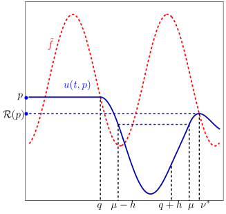
Figure 2: Schematic representation of a $U$-shaped solution and its characteristic points.

Let $\nu^{*}$ be the the smallest $\nu>q$ satisfying (12) and set ${\cal R}(p)=u(\nu^{*},p)$. We refer the reader to Figure 2 below for an illustration of the definition of ${\cal R}$ and some characteristic points involved in our results. The next statement says that ${\cal R}(\tilde{f}([0,\beta]))\subset\tilde{f}([0,\beta))$, in other words, that ${\cal R}(p)>0$ for each $p\in\tilde{f}([0,\beta])$ and the application

$${\cal R}:\tilde{f}([0,\beta])\to\tilde{f}([0,\beta])$$ (13)

is well defined.

Lemma 4

Let $u:[-h,+\infty)\to{\mathbb{R}}$ be a solution of (1), and let $\tau>0$ be a point of local maximum for $u$; moreover, assume that, for some $\epsilon>0$, $u(\tau)\geq u(t)$ for all $t\in[\tau-h,\tau+\epsilon)$. Then $u(\tau)=f(\tau)/|a+b|$ and $\tau^{*}=\tau\pmod{T}\in[0,\beta)$.

Proof 3

The first conclusion of the lemma is evident. We prove the second one by contradiction. Suppose that $\tau^{*}\not\in[0,\beta)$. Then there exists an interval $E=(0,\varepsilon)$, $0<\varepsilon<h$, such that $f(s+\tau)-f(\tau)>0$ and $M=\max\limits_{r\in[\tau-h,\tau]}u(r)\geq u(s+\tau)$ for all $s\in E$. This implies that the function $d(s)=u(s+\tau)-u(\tau)$ satisfies the equation

$$d^{\prime}(s)=ad(s)+f(s+\tau)-f(\tau)$$

for all $s\in E$. Using the variation of constants formula and the equality $d(0)=0$, we get

$$0\geq d(s)\exp(-as)=\int_{0}^{s}\exp(-ar)(f(r+\tau)-f(\tau))dr>0,$$

for all $s\in E$. This contradiction proves that actually $\tau^{*}\in[0,\beta)$.

Note that a partial converse of Lemma 4 is also true:

Lemma 5

Let $u:[-h,+\infty)\to{\mathbb{R}}$ be a solution of (1). If $u(\tau)=\tilde{f}(\tau)=\max\limits_{s\in[\tau-h,\tau]}u(s)$, where $\tau^{*}=\tau\pmod{T}\in[0,\beta)$, then $u$ strictly decreases on $I_{r}:=(\tau,\tau+r)$, where $r=\min\{h,\beta-\tau^{*}\}>0$. In particular, $\tau>0$ is a point of local maximum for $u$.

Proof 4

Indeed, consider the initial value problem $v(\tau)=\tilde{f}(\tau)$ for the equation $v^{\prime}(t)=av(t)+bv(\tau)+f(t)$. The difference $m(t)=v(t)-v(\tau)$ satisfies the equation

$$m^{\prime}(t)=am(t)+f(t)-f(\tau),\quad m(\tau)=0.$$

Thus, by the variation of constants formula, for all $t\in I_{r}$,

$$(v(t)-v(\tau))\exp(-at)=\int_{\tau}^{t}\exp(-as)(f(s)-f(\tau))ds<0,$$

proving that $\tau>0$ is a point of local maximum for $v$ and therefore $u(t)=v(t)$ for all $t\in I_{r}$. The same computation shows that $u(t_{1})=v(t_{1})>v(t_{2})=u(t_{2})$ if $t_{1},t_{2}\in I_{r}$ and $t_{1}<t_{2}$, and therefore $u$ is strictly decreasing on $I_{r}$.

The first recurrence map ${\cal R}$ plays the same role as the Poincaré map in the case of periodic differential equations. The following evident statement summarizes the relations between the delay differential equation (1) and the one-dimensional dynamical system defined by (13).

Lemma 6

For a given solution $u$ of equation (1), the set of all points satisfying the third property of Lemma 2 forms a strictly increasing unbounded sequence $\{\tau_{j},j\in{\mathbb{N}}\}$. Furthermore, $u(\tau_{n+j})={\cal R}^{j}(u(\tau_{n}))$ for all $j\geq 0$ and $n\geq 1$.

We emphasize that, clearly, there is a correspondence between the periodic solutions of (1) and the set of periodic points of ${\cal R}$. In particular, by [3], ${\cal R}$ has at least one fixed point.

2.3 Existence of a compact global attractor

Next, we show how the stability assumptions (9) imply that the semiflow $F^{\mu}:X\times{\mathbb{R}}_{+}\to X$ defined in Subsection 2.1 possesses a compact global attractor.

Lemma 7

Assume that either of the two conditions in (9) holds, that $h<T$, and that the T-periodic continuous function $f$ has sine-like shape. Then, for each $\phi\in C[-h,0]$, there exist $K$, which does not depend on $\phi$, and $t_{0}=t_{0}(\phi)$ such that

$$K\leq u(t,\tau,\phi)\leq f^{*}:=\frac{1}{|a+b|}\max\limits_{t\in[0,T]}f(t),$$ (14)

for all $t\geq t_{0}$ and $\tau\in[0,T)$, where $u(t)=u(t,\tau,\phi)$ denotes the solution of (4), (5).

Proof 5

In view of Lemmas 4 and 6, there is a sequence $\{\tau_{j}\}_{j\in{\mathbb{N}}}$ such that $u(\tau_{j})=-f(\tau_{j})/(a+b)\leq f^{*}$ and $\max\limits_{s\in[\tau_{j}-h,\tau_{j}+\varepsilon_{j}]}u(s)=u(\tau_{j})$, for some $\varepsilon_{j}>0$. Take now two consecutive points $\tau_{k},\tau_{k+1}$ and suppose that

$$u(\tau^{*}):=\max\{u(t):t\in[\tau_{k},\tau_{k+1}]\}>f^{*}.$$

If $\tau^{*}$ is the leftmost point with such a property, then necessarily $\tau^{*}\in\{\tau_{j},j\in{\mathbb{N}}\}$, a contradiction. Therefore $u(t,\tau,\phi)\leq f^{*}$ for all sufficiently large $t$.

By the proof of Lemma 3, we know that for every solution $v:[\tau-h,\infty)\to{\mathbb{R}}$ of (8) there is a real number $\mu$ such that $\mu>2h>0$ and $\|v_{\mu}\|\leq 0.5\|v_{2h}\|$, where $\|\phi\|=\max\{|\phi(s)|:s\in[-h,0]\}.$

On the other hand, in view of Lemma 6, if the ‘universal’ constant $K$ in (14) does not exist, then there are sequences $s_{n}\in[0,T),\ \sigma_{n}\in{\mathbb{R}},\ \phi_{n}(s)\equiv\phi_{n}\in[\min\limits_{t\in{\mathbb{R}}}\tilde{f}(t),\max\limits_{t\in{\mathbb{R}}}\tilde{f}(t)]$, such that the solutions $u(t,s_{n},\phi_{n}):[s_{n}-h,+\infty)\to{\mathbb{R}}$ to (1) satisfy $|u(\sigma_{n},s_{n},\phi_{n})|=\max\limits_{r\in[\sigma_{n}-\mu,\sigma_{n}]}|u(r,s_{n},\phi_{n})|\to\infty$ as $n\to\infty$. Now, the sequence

$$w^{(n)}(s)=\frac{u(\sigma_{n}-\mu+s,s_{n},\phi_{n})}{\max\limits_{r\in[\sigma_{n}-\mu,\sigma_{n}]}|u(r,s_{n},\phi_{n})|}\,,\,s\in[0,\mu],$$

is relatively compact in $C([0,\mu])$. Moreover, every limit function $w$ satisfies equation (8) and $1=|w(\mu)|=\|w_{\mu}\|=\max\limits_{r\in[0,\mu]}|w(r)|\geq\|w_{2h}\|$, a contradiction with the definition of $\mu$.

Corollary 8

Assume all the conditions of Lemma 7 hold. Then the dynamical system $F^{\mu}$ is point dissipative (see [14]). In other words, there exists a positive constant $K_{*}$ such that for each $x\in X$ we can find $t_{0}(x)$ satisfying that $F^{t}x\in S^{1}\times\{\phi:\|\phi\|<K_{*}\}$ for all $t\geq t_{0}(x)$.

Theorem 9

Assume all the conditions of Lemma 7 hold. Then there exists a compact global attractor ${\cal A}(F)$ for $F^{\mu}$.

Proof 6

The existence of the compact global attractor ${\cal A}(F)$ with the mentioned properties is a direct consequence of Corollary 8 and Theorem 5.3 from [15].

It was shown in [3, 10, 24, 32] that if $a+b\not=0$, then equation (1) has at least one $T$-periodic solution or, equivalently, ${\cal A}(F)$ always contains at least one simple closed curve $\Sigma^{1}$ trivially covering the base $S^{1}$. Moreover, ${\cal A}(F)=\Sigma^{1}$ under some additional assumptions (e.g. if one of the following three conditions is satisfied: i) $|b|+a<0$;  ii) $(|a|+|b|)h<1,\ b<-a<0$;  iii) $0<-bh<3/2$ and $\ a=0$). In general, ${\cal A}(F)$ does not coincide with $\Sigma^{1}$: as it was proved in [32] (see also Section 3.1 below), the global attractor can have several periodic orbits. Moreover, in Section 3.2 of the paper we will show that ${\cal A}(F)$ can even possess an infinite set of periodic solutions as well as some solutions with ‘chaotic’ behavior.

2.4 Continuity of the return map

Again, we will assume all the conditions of Lemma 7 hold. We begin by considering the initial value problem $u(\tau)=\tilde{f}(\tau)$ for the ordinary differential equation

$$u^{\prime}(t)=(a+b)u(t)+f(t).$$ (15)

Clearly, there exists some $\delta>0$ such that $f(t)-f(\tau)$ does not change sign on each of the open intervals $(\tau-\delta,\tau)$, $(\tau,\delta+\tau)$. A straightforward computation shows that the solution $u$ of the mentioned initial value problem satisfies, for all $0<|t-\tau|<\delta$,

$$\frac{u(t)-u(\tau)}{t-\tau}(f(t)-f(\tau))=\frac{1}{t-\tau}\int_{\tau}^{t}e^{(a+b)(t-s)}(f(t)-f(\tau))(f(s)-f(\tau))ds>0.$$

This relation implies the following result:

Lemma 10

If $\tau\in(0,\beta)$ [respectively, $\tau\in(\beta,T)$] then the solution $u$ of the initial value problem $u(\tau)=\tilde{f}(\tau)$ for (15) has a strict local maximum [respectively, strict local minimum] at $\tau$. Moreover, $\tau$ is the unique critical point of $u$ in some open neighbourhood of $\tau$. If $\tau=\beta$, then $u^{\prime}(t)>0$ for all $t$ in some punctured neighbourhood of $\beta$. If $\tau=T$, then $u^{\prime}(t)<0$ for all $t$ in some punctured neighbourhood of $T$.

Proof 7

Suppose, for example, that $\tau=\beta$. Then $u(\tau)=0$ and $u(t)<0$ for $t\in(\tau-\delta,\tau)$. Since $a+b<0$ this implies that $u^{\prime}(t)>0$ for $t\in(\tau-\delta,\tau)$. Similarly, $u(t)>0$ for $t\in(\tau,\delta+\tau)$. If we suppose that $u^{\prime}(s_{0})=0$ for some $s_{0}\in(\tau,\delta+\tau)$ then $u(t)$ is strictly decreasing on $(\beta,s_{0})$ (since $f(t)$ is strictly increasing on the same interval), a contradiction. The other cases can be established in a similar fashion.

Set $K=\tilde{f}([0,\beta])$. The goal of this subsection is to describe the continuity properties of the map ${\cal R}:K\to K$. First, we will analyse the trajectory of the solution $u(s,p)$ on the interval $(q,\nu^{*})$ (see Subsection 2.2 and Figure 2 for the notation related to the definition of ${\cal R}$). We next state an assumption that will guarantee good continuity properties of ${\cal R}$ and admits practical verification:

(M) For each $p\in K$ it holds that $u(s,p)<u(\nu^{*},p)$ for all $s\in[\nu^{*}-h,\nu^{*})$.

Note that the last assumption needs to be checked only for those $p$ satisfying ${\cal R}(p)<p$ because of the following simple result:

Lemma 11

Suppose that $p\in K$ and ${\cal R}(p)\geq p$. Then

$$u(s,p)<u(\nu^{*},p)\,,\ s\in[\nu^{*}-h,\nu^{*}).$$ (16)

Proof 8

If ${\cal R}(p)>p$, the result is a consequence of the definition of ${\cal R}$. Assume that ${\cal R}(p)=p$ and (16) does not hold. This means that, if $p=\tilde{f}(q)$, then $\nu^{*}-q\leq h$. But this is a contradiction, because Lemma 4 ensures that $\nu^{*}-q\geq T>h$ if ${\cal R}(p)=p$.

Lemma 12

Assume that (M) holds. Then for each $p=\tilde{f}(q)\in K$ there exists a maximal non-empty interval $(\mu(q),\nu^{*})$ such that $u(t,p)>u(s,p),s\in[t-h,t)$ for all $t\in(\mu(q),\nu^{*})$. In particular, $u^{\prime}(t,p)>0$ (possibly, except for one point $s=\beta+jT$ where $u(s,p)=0$) and $u(t,p)$ satisfies (15) on $(\mu(q),\nu^{*})$.

Proof 9

Indeed, otherwise there exist increasing sequences $s_{n}<t_{n}<\nu^{*},\ s_{n},t_{n}\to\nu^{*}$ such that $u(t_{n})\leq u(s_{n})=\max\{u(s),s\in[s_{n}-h,t_{n}]\}.$ However, this contradicts the definition of $\nu^{*}$.

As a consequence, $u(t,p)$ satisfies (15) on $(\mu(q),\nu^{*})$. By Lemma 10, $u^{\prime}(s,p)=0$ if and only if $s=\beta+jT$ for some integer $j$ and $u(s,p)=\tilde{f}(\beta)=0$.

Corollary 13

For each $p\in K$, the inequality ${\cal R}(p)<\max\{\tilde{f}(t),\ t\in{\mathbb{R}}\}$ holds.

Proof 10

Indeed, if ${\cal R}(p)=\max\{\tilde{f}(t),\ t\in{\mathbb{R}}\}\geq p$ for some $p\in K$, Lemmas 11 and 12 imply that $u(t,p)$ satisfies (15) and increases on some left-hand side neighbourhood of $\nu^{*}=0\pmod{T}$. However, this contradicts the last assertion of Lemma 10.

Corollary 14

With the notations of Lemma 12, $\mu(\beta)=\beta$.

Proof 11

Lemma 10 implies that the solution of the initial problem $u(\beta,0)=0$ increases on some right-hand side neighbourhood of $\beta$. Therefore the graph of $u(t,0)$ increases until its first intersection at some point $(z,{\cal R}(0)),\ z\in(\beta,\beta+T),$ with the decreasing part of the graph of the function $\tilde{f}:[T,\beta+T)\to(0,+\infty)$.

Theorem 15

Assume that (M) holds and $\beta<h$. Let $p_{0}=\tilde{f}(q_{0})$ be a point of discontinuity for ${\cal R}$. Then $u(\beta+jT,p_{0})=0$ for some $\beta+jT\in[\mu(q_{0}),\nu^{*}(q_{0}))$ with $j\in{\mathbb{N}}$. Furthermore,

$${\cal R}(p_{0})={\cal R}(0),\quad\mbox{$\displaystyle\liminf_{p\to p_{0}}{\cal R}(p)=0.$}$$

Proof 12

Indeed, due to the continuous dependence of solutions on the initial values, $u^{\prime}(t,p)$ converges uniformly to $u^{\prime}(t,p_{0})$ on $[\mu(q_{0}),\nu^{*}(q_{0})]$ as $p\to p_{0}$. By Lemma 4 and Corollary 13, $\nu^{*}(q_{0})\in(j_{0}T,j_{0}T+\beta)$ for some $j_{0}$. Set $\mu_{*}(q_{0})=\max\{j_{0}T,\mu(q_{0})\}$. Then Lemma 12 and Corollary 14 assure that for every $\delta>0$ it holds that $u^{\prime}(t,p)>0$ for all $t\in[\mu_{*}(q_{0})+\delta,\nu^{*}(q_{0})-\delta)$ if $p$ is sufficiently close to $p_{0}$. This implies that $u(t,p)>u(s,p),$ $\ s\in[t-h,t)$, for $t\in(\mu_{*}(q_{0})+\delta,\nu^{*}(q_{0})-\delta)$ and therefore $u(t,p)$ has a local maximum point $\hat{\nu}(p)$ such that $\hat{\nu}(p)\to\nu^{*}(p_{0})$ as $p\to p_{0}$. In addition, $u(t,p)$ is strictly monotone in some left and in some right neighbourhoods of $\hat{\nu}(p)$ and $u(\hat{\nu}(p),p)=\max\{u(s,p),\ s\in$ $[\hat{\nu}(p)-h,\hat{\nu}(p)]\}$.

Now, since $\beta<h$, by Lemma 4, $\hat{\nu}(p)$ is the absolute maximum point of $u(t,p)$ on the interval $(j_{0}T,\beta+j_{0}T)$ containing $\nu^{*}(q_{0})$. Therefore, if we suppose that ${\cal R}$ has a discontinuity at $p_{0}$, it should exist a sequence $p_{k}=\tilde{f}(q_{k})\to p_{0}=\tilde{f}(q_{0})$ and a positive integer $j_{1}<j_{0}$ such that $\nu^{*}(q_{k})\in[j_{1}T,\beta+j_{1}T)$ and $\nu^{*}(q_{k})\to\mu^{*}$ $\neq\nu^{*}(q_{0})\pmod{T}.$ Since $u(\nu^{*}(q_{k}),p_{k})=\max\{u(s,p_{k}),\ s\in$ $[\nu^{*}(q_{k})-h,\nu^{*}(q_{k})]\}$, in view of the continuous dependence of $u(t,p)$ on the initial data, we conclude that

$$u(\mu^{*},p_{0})=\max\{u(s,p_{0}),\ s\in[\mu^{*}-h,\mu^{*}]\}.$$

Now, if $\mu^{*}<\beta+j_{1}T$ (i.e. $u(\mu^{*},p_{0})\not=0$), then by Lemma 4, $u(\mu^{*},p_{0})=\max\{u(s,p_{0}),\ s\in[\mu^{*}-h,\beta+j_{1}T]\}$ and $[j_{1}T,\beta+j_{1}T)\ni\mu^{*}=\nu^{*}(q_{0})\in[j_{0}T,\beta+j_{0}T)$, a contradiction.

Therefore $\mu^{*}=\beta+j_{1}T$,

$$\max\{u(s,p_{0}),\ s\in[\mu^{*}-h,\mu^{*}]\}=u(\mu^{*},p_{0})=u(\beta+j_{1}T,p_{0})=0,$$

so that ${\cal R}(p_{0})={\cal R}(0)$ and ${\cal R}(p_{k})=u(\nu^{*}(q_{k}),p_{k})\to u(\mu^{*},p_{0})=u(\beta+j_{1}T,p_{0})=0$.

Theorem 15 allows us to find sufficient conditions for the continuity of ${\cal R}$ in some subsets of its domain $K$. We address this task in the next three colloraries.

Corollary 16

If $h\in(\beta,T)$, ${\cal R}(p_{0})\geq p_{0},$ and ${\cal R}(p_{0})\not={\cal R}(0)$, then ${\cal R}$ is continuous at $p_{0}$.

Proof 13

It is a consequence of Lemma 11 and Theorem 15.

Corollary 17

Suppose that $h\in(\beta,T)$, and let $p=\tilde{f}(q)\in K.$ If the following inequality holds:

$$\int_{0}^{h}e^{as}(f(q+h-s)-f(q))ds\geq 0,$$ (17)

then ${\cal R}$ is continuous at $p$, ${\cal R}(p)\geq p,$ and $\nu^{*}(q)$ $\in(T,T+\beta).$ Moreover, there exists $r\in(q,q+h]$ such that $u(r,p)=p$, $u^{\prime}(r,p)>0$, and $u(t,p)<p$ for all $t\in(q,r]$.

Proof 14

Since ${\cal R}(p)>0$ for all $p\in K$, it suffices to take $p>0$. Consider the solution $u(t,p)$ on the interval $I_{q}=(q,q+h]$. If $u(t,p)\leq p$ for all $t\in I_{q}$, and (17) holds, we obtain

$$u(q+h,p) =e^{ah}p+\int_{q}^{q+h}e^{a(h+q-s)}[bp+f(s)]ds=$$

$$=e^{ah}p+p\frac{b}{a}(e^{ah}-1)+\int_{0}^{h}e^{as}f(q+h-s)ds\geq p.$$

This shows that $u(r,p)=p$ at some leftmost point $r\in(q,q+h]$ where $u^{\prime}(r,p)\geq 0$. If $u^{\prime}(r,p)=0$, then $p=u(r,p)=\tilde{f}(r)$, so that $r\in(\beta,T)$ and therefore, repeating the computation in the proof of Lemma 5, we find that $u(t,p)>p$ for $t\in(\beta,r)$, a contradiction. Thus $u^{\prime}(r,p)>0$ so that, by the definition of $\nu^{*}(q)$, the solution $u(t,p)$ is increasing on the interval $(r,\nu^{*}(q))$.

Moreover, since $h<T$ and $u(t,p)>p\geq 0$ on $(r,\nu^{*}(q))$, the graph of the solution does not intersect the set $\{(\beta+jT,0):j\geq 1\}$. Hence, by Theorem 15, ${\cal R}$ is continuous at $p$ if (17) holds.

Corollary 18

Suppose that $h\in(\beta,T)$, $b<0$. Then ${\cal R}$ is continuous at the point $p$, if

$${\cal R}(p)\not={\cal R}(0)\quad\mbox{and}\quad\int_{0}^{h}e^{as}(f(\nu^{*}(q)-s)-f(\nu^{*}(q)))ds<0.$$ (18)

Proof 15

We claim that $u(s,p)<u(\nu^{*},p)$ for all $s\in[\nu^{*}-h,\nu^{*})$. Indeed, otherwise $\max\{u(s,p),s\in[t-h,t]\}\geq{\cal R}(p)$ for all $t\in[\nu^{*}-h,\nu^{*}]$ so that

$${\cal R}(p) =e^{ah}u(\nu^{*}-h,p)+\int_{\nu^{*}-h}^{\nu^{*}}e^{a(\nu^{*}-s)}[b\max_{w\in[s-h,s]}u(w,p)+f(s)]ds\leq$$

$$\leq e^{ah}{\cal R}(p)+\int_{\nu^{*}-h}^{\nu^{*}}e^{a(\nu^{*}-s)}[b{\cal R}(p)+f(s)]ds=$$

$$=e^{ah}{\cal R}(p)+\int_{0}^{h}e^{as}[b{\cal R}(p)+f(\nu^{*}-s)]ds<{\cal R}(p),$$

a contradiction. Thus condition (M) is satisfied and Theorem 15 implies the continuity of ${\cal R}$ at $p$ once ${\cal R}(p)\not={\cal R}(0)$.

We illustrate the application of Corollaries 17 and 18 with an example that we will consider in Section 3.2.

Example 19

Consider the equation

$$u^{\prime}(t)=0.32u(t)-\max_{t-3\pi/2\leq s\leq t}u(s)+1-\sin t.$$ (19)

We can easily check that the second condition in (9) holds. Since $\beta=\pi<h=1.5\pi<T=2\pi$, we can apply Corollaries 17 and 18 to conclude that ${\cal R}$ is continuous on the interval $[0,0.9]\subset K=[0,2(a+b)^{-1}]\approx[0,2.94118]$, where ${\cal R}(p)>p$ (by Corollary 17) and ${\cal R}$ is continuous at each point of the set ${\cal R}^{-1}([1.43\dots,2.94\dots]\setminus{{\cal R}(0)})$ (by Corollary 18). The graph of the return map for equation (19) is numerically plotted in Figure 4. The next result shows that the graph in this figure is a continuous curve at least till its first intersection with the diagonal. Theorem 28 in Section 3 describes in more detail the main continuity properties of the return map for (19).

Corollary 20

Assume that either of the stability conditions in (9) holds and suppose that $h\in(\beta,T)$. Then there are $\delta>0$ and $p^{*}$ such that ${\cal R}(p^{*})=p^{*}$ and ${\cal R}(p)>p$ for all $p\in[0,p^{*})$. Furthermore, ${\cal R}$ is continuous on $[0,p^{*}+\delta)$. If, in addition, (M) is satisfied and $[0,c)\subset K$ is the maximal half-open interval where ${\cal R}$ is continuous then either $[0,c]=K$ and $\inf{\cal R}(K)>0$ or ${\cal R}(c-)=0,\ {\cal R}(c)={\cal R}(0)>0$.

Proof 16

In view of Lemma 10 and Corollary 13, the graph of $u(t,0)$ increases until its first intersection at some point $(z,{\cal R}(0)),\ z\in(T,\beta+T)$ with the decreasing part of the graph $\Gamma$ of $\tilde{f}:(T,\beta+T)\to(0,+\infty)$. Since $u(t,0)$ has a strict maximum at $z$, it follows that

$$u(z,0)>u(s,0),\ \mbox{for all}\ s\in[z-h,z+\epsilon]\setminus\{z\},$$

for all small $\epsilon>0$, and hence we conclude that for $p>0$ close to $0$ the solutions $u(t,p)$ have also strict maxima at some points close to $z$. Therefore the continuous dependence of $u(t,p)$ on the variables $(t,p)$ implies that the point $(\nu^{*}(q),{\cal R}(p))$ changes continuously belonging to $\Gamma$ while ${\cal R}(p)\geq p$. By the continuity of $u(t,p)$, our argument still works when $p$ belongs to some right-hand neighbourhood of the least fixed point $p^{*}$.

Finally, if (M) holds, then condition ${\cal R}(p)\geq p$ can be omitted in the above argumentation and ${\cal R}$ has a continuous graph until the first intersection of its closure with the real axis at some point $c$, where ${\cal R}(c-)=0,\ {\cal R}(c)={\cal R}(0)>0$.

Corollary 20 provides an alternative proof of the existence of at least one $T-$periodic solution for equation (1) with sine-like $T$-periodic continuous function $f(t)$. In [3] this result was obtained by using the topological degree method.

2.5 Differentiability of the return map

Hereafter, we again assume that all the conditions of Lemma 7 hold and $\beta<h$. It is not difficult to prove the differentiability (possibly, one-side differentiability) of the return map ${\cal R}$ in the case when the graph of $u=u(t,p)$ on the interval $(q,\nu^{*}(q))$ is $U$-shaped in the following sense:

Definition 21

We will say that the solution $u(t,p)$ is $U$-shaped if on the interval $\Omega_{q}=(q,\nu^{*}(q))$ it has only one critical point, in which it reaches its minimal value, and if in some left-side neighborhood of $\nu^{*}$, $u(t,p)$ satisfies the ordinary differential equation (15). Set $U(t,p)=\max\{u(s,p),s\in[t-h,t]\}.$ If $u(t,p)$ is $U$-shaped, then the interval $\Omega_{q}$ can be represented as the disjoint union of the subintervals $I_{1}=(q,\lambda(q)]$, $I_{2}=(\lambda(q),\mu(q)]$ and $I_{3}=(\mu(q),\nu^{*}(q))$, where either $\lambda(q)=q+h,$ or $\lambda(q)=\mu(q)$ and $I_{2}=\emptyset$, such that $U(t,p)=p$ on $I_{1}$, $U(t,p)=u(t-h,p)$ on $I_{2}$, and $U(t,p)=u(t,p)$ on $I_{3}$.

Due to Theorem 15, ${\cal R}$ is continuous at $p$ if $u(t,p)$ is $U$-shaped and its graph does not intersect the set $\{(\beta+kT,0),k\geq 1\}\subset{\mathbb{R}}^{2}$.

Assuming $u(t,p)$ is $U$-shaped, we introduce the following variational equation along $u(t,p)$:

$$w^{\prime}(t)=\begin{cases}aw(t)+bw(q),&\text{if $q\leq t\leq\lambda(q)$,}\\ aw(t)+bw(t-h),&\text{if $\lambda(q)\leq t<\mu(q)$,}\\ (a+b)w(t),&\text{if $\mu(q)\leq t<\nu^{*}(q),$}\end{cases}$$ (20)

where $\lambda(q)\in\{q+h,\mu(q)\}$.

Let $v$ denote the fundamental solution of the linear delay-differential equation (10). Then, if $w(t)$ satisfies the variational equation (20), we obtain (see [16, Chapter 1, Theorem 6.1]) hat $w(\nu^{*}(q))=\Delta(q)w(q),$ where

$$\Delta(q)=\left(v(\mu-q)+b\int_{\mu-q-h}^{\mu-q}v(s)ds\right)e^{(a+b)(\nu^{*}-\mu)}.$$

To simplify and shorten our proofs, hereafter we assume the following additional assumption that is fulfilled in the example considered in Subsection 3.2:

(T) $f$ is a $C^{1}$-smooth $T$-periodic function having exactly two critical points on each half-open interval of length $T$. Moreover, $a>0$, $b<0$ and $h\in(\beta,T)$.

Using (T), we can easily establish that $u(t,p)$ has at most one critical point on the time interval $(q,T]\cap(q,q+h)$. If $p=0$, this fact follows from Lemma 10. Next, Lemma 5 shows that $u(t,p)$ with $p>0$ decreases on some maximal non-empty interval $I\supset(q,\min\{q+h,\beta\})$. In fact, if $\hat{q}>\beta$ is the leftmost point satisfying $\tilde{f}(\hat{q})=p$, then

$$u^{\prime}(t,p)=au(t,p)+bp+f(t)<(a+b)p+f(q)=0,$$

for all $t\in(q,\min\{q+h,\hat{q}\}]$.

If $u(t,p)$ has a leftmost critical point $t_{m}\in(\hat{q},q+h)$ then $0\leq u^{\prime\prime}(t_{m})=f^{\prime}(t_{m})$ implying that $\beta<t_{m}\leq T$ and $0<u^{\prime\prime}(t_{m})$ if $t_{m}<T$. In particular, $u(t,p)$ can have at most one critical point on $(q,T)$. Now, suppose that $u^{\prime}(T,p)=0$ and $t_{m}<T<q+h$. Then $u(t,p)<p$ for all $t\in(q,T]$ so that $v(t)=u^{\prime}(t,p)$ satisfies $v^{\prime}(t)=av(t)+f^{\prime}(t),\ v(T)=0,$ in some small neighbourhood of $T$. Since $f^{\prime}(t)$ is changing its sign at $T$ from positive to negative, $v(t)$ is negative in some small punctured vicinity of $T$. Thus $u(t,p)$ should have an additional local maximum point between $t_{m}$ and $T$, a contradiction. In this way, $u(t,p)$ can have at most one critical point on $(q,T]\cap(q,q+h)$.

The above reasoning is useful in proving the following result:

Lemma 22

Assume that (T) and all the conditions of Lemma 7 hold. If (17) is true then the graph of $u=u(t,p)$ is $U$-shaped.

Proof 17

With the notations of Corollary 17 and the above comments, it suffices to establish that $t_{m}$ is the unique critical point of $u(t,p)$ on the interval $(q,r)$. Indeed, if $u(t,p)$ has a different critical point $t_{*}\in(T,r)\subset(T,\beta+T)$, then $u^{\prime\prime}(t_{*},p)=f^{\prime}(t_{*})<0$ and therefore $t_{*}$ is the unique critical point of $u(t,p)$ on $(T,r)$ where a local maximum is reached. Thus $u^{\prime}(r,p)<0$, which is impossible by Corollary 17.

By the same arguments, if $q+h>T$ then $u(t,p)$ can have at most one additional critical point on $(T,q+h]$ where a local maximum is reached. Clearly, this can happen only when $u(t,p)<p$ for $t\in(q,q+h]$. Furthermore, suppose that there exists the leftmost point $r\in(q,q+h]$ such that $u(r,p)=p$. We claim that then the inequality (17) is necessarily satisfied. Indeed, otherwise the solution $u_{p}(t)$ of the initial value problem $u^{\prime}(t)=au(t)+bp+f(t),$ $u_{p}(q)=p$ satisfies $u_{p}(q+h)<p$ (observe that the inequality $u_{p}(q+h)\geq p$ amounts to (17)). Thus $u_{p}(t)$ reaches its absolute maximum on $[r,q+h]$ at some point $t^{*}\in(T,q+h]$. Since $h<T$ this implies that $f(t^{*})>f(q)$ and, consequently, $0=u^{\prime}_{p}(t^{*})=au(t^{*})+bp+f(t^{*})>ap+bp+f(t^{*})=f(t^{*})-f(q)>0$, a contradiction.

Hence, under the assumptions of Lemma 22, $\mu(q)\leq q+h$ if and only if the inequality (17) holds. For simplicity, it is convenient to consider the following assumption:

(C) The set of all $q\in[0,\beta)$ satisfying inequality (17) is a nonempty interval $S=(\beta_{1},\beta)$.

For example, condition (C) holds for equation (19) introduced in Example 19 with $\beta_{1}\approx 0.39289$ (see Example 24).

By the implicit function theorem, if (17) and (C) hold then the equation $u(t,p(q))=p(q)$, where we denote $p=\tilde{f}(q)=p(q)$, has a unique solution $t=\lambda(q)\in(q,q+h],$ smoothly depending on $q\in[\beta_{1},\beta)$. Also $\lambda(q)=\mu(q)$ if $q\in[\beta_{1},\beta)$ and $\lambda(q)=q+h$, if $q\leq\beta_{1}$.

Next, if $q\in(\beta_{1},\beta)$, then

$$p=e^{a(\lambda(q)-q)}p+\int_{q}^{\lambda(q)}e^{a(\lambda(q)-s)}(bp+f(s))ds,$$ (21)

so that

$$1=\left(p(a+b)+f(\lambda(q))\right)\partial_{p}\lambda(q)+\left(1+\frac{b}{a}\right)e^{a(\lambda(q)-q)}-\frac{b}{a},$$

where $\partial_{p}$ denotes the partial derivation with respect to $p$. Next, for $q\in(\beta_{1},\beta)$,

$${\cal R}(p)=u(\nu^{*}(q),p)=pe^{(a+b)(\nu^{*}(q)-\lambda(q))}+\int^{\nu^{*}(q)}_{\lambda(q)}e^{(a+b)(\nu^{*}(q)-s)}f(s)ds,$$

where $\nu^{*}$ is $C^{1}$-smooth function of $q$ as the solution of the equation $F(\nu,q)=0,$ where $F(\nu,q)=au(\nu,p(q))+bp(q)+f(\nu),\ \partial_{\mu}F(\nu,p)=au^{\prime}(\nu,p)+f^{\prime}(\nu)=f^{\prime}(\nu)<0$. A straightforward computation shows that

$${\cal R}^{\prime}(p)= u^{\prime}(\nu^{*}(q),p)\partial_{p}\nu^{*}(q)+e^{(a+b)(\nu^{*}(q)-\lambda(q))}-$$

$$p(a+b)e^{(a+b)(\nu^{*}(q)-\lambda(q))}\partial_{p}\lambda(q)-e^{(a+b)(\nu^{*}(q)-\lambda(q))}f(\lambda(q))\partial_{p}\lambda(q)=$$

$$e^{(a+b)(\nu^{*}(q)-\lambda(q))}-e^{(a+b)(\nu^{*}(q)-\lambda(q))}\left(p(a+b)+f(\lambda(q))\right)\partial_{p}\lambda(q)=$$

$$e^{(a+b)(\nu^{*}(q)-\lambda(q))}\left(\left(1+\frac{b}{a}\right)e^{a(\lambda(q)-q)}-\frac{b}{a}\right)=\Delta(q(p)).$$

As a consequence, we have the following result:

Theorem 23

Assume (T) and (C) hold, and let $q\in(\beta_{1},\beta)$. Then $\mu(q)=\lambda(q)$ and

$${\cal R}^{\prime}(p)=e^{(a+b)(\nu^{*}(q)-\mu(q))}\left(\left(1+\frac{b}{a}\right)e^{a(\mu(q)-q)}-\frac{b}{a}\right)=\Delta(q(p)).$$ (22)

Therefore, $b>a/(e^{-ah}-1)$ implies that ${\cal R}^{\prime}(p)>0$ for all $p\in(0,\tilde{f}(\beta_{1}))\subset(0,p^{*})$. On the other hand, if $b<a/(e^{-ah}-1)$ and the only root of equation

$$f(\tau)+b\int_{0}^{\frac{1}{a}\ln\frac{b}{a+b}}e^{-au}f(u+\tau)du=0$$ (23)

is $\tau=q_{0}\in(\beta_{1},\beta)$, then ${\cal R}^{\prime}(p)>0$ for $p\in(0,\tilde{f}(q_{0}))$ and ${\cal R}^{\prime}(p)<0$ for $p\in(\tilde{f}(q_{0}),\tilde{f}(\beta_{1}))$.

Proof 18

Since $\lambda(q)-q<h$ for all $q\in(\beta_{1},\beta)$, it follows that $\Delta(q)>0$ for all $q\in(\beta_{1},\beta)$ if $h\leq(1/a)\ln(b/(b+a)).$

On the other hand, if $h>(1/a)\ln(b/(b+a))$, then by the intermediate value theorem, there is $q_{0}\in(\beta_{1},\beta)$ such that

$$\lambda(q_{0})-q_{0}=\frac{1}{a}\ln\left(\frac{b}{b+a}\right)$$

and therefore ${\cal R}^{\prime}(p(q_{0}))=0$. Furthermore, it follows from (21) that $q_{0}$ satisfies (23), which proves the uniqueness of $q_{0}$ (under our assumptions). Hence,

$$\lambda^{*}(q)-q<\frac{1}{a}\ln\left(\frac{b}{b+a}\right),\ \mbox{for}\ \,q\in(q_{0},\beta);\quad\lambda(q)-q>\frac{1}{a}\ln\left(\frac{b}{b+a}\right),\ \mbox{for}\ q\in(\beta_{1},q_{0}),$$

which finalises the proof.

Example 24

For the equation (19) considered in Example 19, we get $\beta=0.5\pi$, $b<a/(e^{-ah}-1)$, and we numerically find $\beta_{1}\approx 0.39289$, $\tilde{f}(\beta_{1})\approx 0.90754$, $q_{0}\approx 1.18459422$, $\tilde{f}(q_{0})\approx 0.10831425.$ Thus, the return map ${\cal R}$ is $C^{1}$-smooth on the interval $[0,0.9]$, where it has a unique critical point $p_{c}=\tilde{f}(q_{0})$. Moreover, ${\cal R}$ reaches its absolute maximum at $p_{c}$. See Figure 4.

It is quite remarkable that the expression for ${\cal R}^{\prime}(p)$ in (22) does not depend on the derivatives $\partial_{q}\nu^{*}(q)$ and $\partial_{q}\mu(q)$. As one can see in the proof of our next result, it is due to the following three circumstances: a) that $u^{\prime}(s,p)=0$ for all $s\in[q-h,q]$ (this eliminates the dependence on $\partial_{q}\mu(q)$); b) that $u^{\prime}(\nu^{*}(q),p)=0$ (this eliminates the dependence on $\partial_{q}\nu^{*}(q)$); and c) that the graph of $u(t,p)$ is $U-$shaped.

The next result can be viewed as a natural extension of Theorem 23 for $q\leq\beta_{1}$.

Theorem 25

Suppose that assumptions (T) and (C) are satisfied, equation (23) has a unique root $\tau\in(\beta_{1},\beta)$, and there is $\alpha\in(0,\beta)$ such that the solutions $u(t,p(q))$ of equation (1) are $U$-shaped for all $q\in(\alpha,\beta]$. If $\Delta(q)<0$ for $q\in(\alpha,\beta_{1}]$, then there is an increasing sequence (either finite or infinite) of real numbers $p_{i}$, with $0<\tilde{f}(\tau)<p_{1}<\dots<p_{j}<\dots<\tilde{f}(\alpha),$ such that ${\cal R}$ is differentiable on the intervals $D_{1}=[0,p_{1}),\dots,D_{j}=[p_{j-1},p_{j}),\dots$, strictly increasing on the interval $(0,\tilde{f}(\beta_{1}))$, and strictly decreasing on the interval $(\tilde{f}(\beta_{1}),p_{1})$ and on every $D_{j},\ j>1.$ Moreover, ${\cal R}(p)$ is right continuous at $p_{i}$ and ${\cal R}(p_{j}-)=0,\ {\cal R}(0)={\cal R}(p_{j})$. Finally, ${\cal R}^{\prime}$ is continuous on every $D_{j}$ and ${\cal R}^{\prime}(p)=\Delta(q(p))$, ${\cal R}^{\prime}(p_{j}-)<{\cal R}^{\prime}(p_{j}+)$.

Proof 19

By Theorem 15, ${\cal R}$ is continuous at $p$ if $u(t,p)$ is $U$-shaped and if the graph of $u(t,p)$ does not intersect the set $\{(\beta+kT,0):k\in{\mathbb{N}},\,k\geq 1\}$ on the interval $(q,\nu^{*}(q))$. Suppose that ${\cal R}$ is continuous at a point $p_{0}=p(q_{0})$, with $q_{0}<\beta_{1}.$ We claim that ${\cal R}^{\prime}(p_{0})=\Delta(q_{0})$. Indeed, since $q_{0}<\beta_{1}$, we have that $\lambda(q_{0})=q_{0}+h<\mu(q_{0})$ and therefore, for all $p$ close to $p_{0}$, it holds

$${\cal R}(p) =u(\nu^{*}(q),p)=u(\mu(q),p)e^{(a+b)(\nu^{*}(q)-\mu(q))}+\int^{\nu^{*}(q)}_{\mu(q)}e^{(a+b)(\nu^{*}(q)-s)}f(s)ds,$$

$${\cal R}^{\prime}(p) =e^{(a+b)(\nu^{*}(q)-\mu(q))}\left(\partial_{p}(u(\mu(q),p))-((a+b)u(\mu(q),p)+f(\mu(q))\partial_{p}\mu(q)\right).$$

Now, we have to calculate the partial derivative $\partial_{p}(u(\mu(q),p))$. A key observation here is that, since $u(t,p)$ is $U$-shaped, it satisfies the following delay differential equation on $[q,\mu(q)]$:

$$u^{\prime}(t)=au(t)+bu(t-h)+f(t),\ t\in[q,\mu(q)],\quad u(s)=p,\ s\in[q-h,q].$$

Thus, using the above mentioned fundamental solution $v$, from [16, Section 1.6] we obtain that

$$u(\mu(q),q)=v(\mu(q)-q)p+bp\int_{q-h}^{q}v(\mu(q)-s-h)ds+\int_{q}^{\mu(q)}v(\mu(q)-s)f(s)ds.$$

As a consequence, since $u(\mu(q),p)=u(\mu(q)-h,p)$, we find that

$$\partial_{p}u(\mu(q),q) =u^{\prime}(\mu(q),q)\partial_{p}\mu(q)+v(\mu(q)-q)+b\int_{q-h}^{q}v(\mu(q)-s-h)ds+$$

$$\left(-v^{\prime}(\mu(q)-q)p-v(\mu(q)-q)f(q)+bpv(\mu(q)-q-h)-bpv(\mu(q)-q)\right)\partial_{p}q=$$

$$u^{\prime}(\mu(q),q)\partial_{p}\mu(q)+v(\mu(q)-q)+b\int_{q-h}^{q}v(\mu(q)-s-h)ds=$$

$$\left[(a+b)u(\mu(q),q)+f(\mu(q))\right]\partial_{p}\mu(q)+v(\mu(q)-q)+b\int_{q-h}^{q}v(\mu(q)-s-h)ds.$$

In this way,

$${\cal R}^{\prime}(p)=e^{(a+b)(\nu^{*}(q)-\mu(q))}\left[v(\mu(q)-q)+b\int_{q-h}^{q}v(\mu(q)-s-h)ds\right]=\Delta(q).$$ (24)

Next, integrating equation (20) we find that $\Delta(q)$ is a combination of some elementary functions depending on $a$, $b$, $h$, $\lambda(q)$, $\mu(q)$ and $\nu^{*}(q)$. The continuous dependence of $\lambda(q)$, $\mu(q)$ and $\nu^{*}(q)$ on $q$ belonging to some small neighbourhood ${\cal O}$ of $q_{0}$ implies the continuity of ${\cal R}^{\prime}(p)=\Delta(q)$ in ${\cal O}$.

Observe also that the sign of ${\cal R}^{\prime}(p)$ is completely defined by the factor given in brackets in (24). In view of the $U$-shaped form of $u(t,p)$, the function $\mu(q)$ is $C^{1}$-smooth so that the aforementioned factor depends continuously on $p$. Differently, $\nu^{*}(q)$ is discontinuous at the preimages of the discontinuity points $p_{j}=\tilde{f}(q_{j})$ of ${\cal R}$. Assuming that there exist ${\cal R}^{\prime}(p_{j}+)$ and ${\cal R}^{\prime}(p_{j}-)$, we find immediately that

$${\cal R}^{\prime}(p_{j}+)={\cal R}^{\prime}(p_{j}-)e^{(a+b)(\nu^{*}(\beta)-\beta)}<{\cal R}^{\prime}(p_{j}-).$$

By Corollary 20, either ${\cal R}$ is continuous on $K$ or there exists a leftmost discontinuity point $p_{1}$. In the first case, ${\cal R}$ has a unique critical point $\tilde{f}(\tau)$ on $K$ and $\nu^{*}(q)<T+\beta$ for all $q$. In the second case, ${\cal R}$ is continuous and strictly decreasing on $[\tilde{f}(\tau),p_{1})$, with ${\cal R}(p_{1}-)=0,\ {\cal R}(0)={\cal R}(p_{1})$.

Next, we claim that $\nu^{*}(q)>\beta+T$ for $p>p_{1}$. Indeed, if $\nu^{*}(\hat{q})<\beta+T$ for some $\hat{p}=\tilde{f}(\hat{q})>p_{1}$, then the negativity of ${\cal R}^{\prime}(p)$ yields $\nu^{*}(q)<\beta+T$ for all $q\in(\hat{q},\beta)$, a contradiction. Therefore, considering the $U$-shaped form of $u(t,p)$ and the inequality ${\cal R}^{\prime}(p)<0$, we conclude that the graph of $u(t,p)$ does not contain the point $(\beta+T,0)$ for $p>p_{1}$. This allows us to repeat the argumentation of Corollary 20 for the case when $\nu^{*}(q)\in(2T,\beta+2T)$. In particular, we obtain that ${\cal R}$ is continuous and strictly decreasing on some maximal open right neighbourhood ${\cal O}_{1}$ of $p_{1}$ and that, if $p_{2}:=\sup{\cal O}_{1}$ is an interior point of $K$, then ${\cal R}(p_{2}-)=0,\ {\cal R}(0)={\cal R}(p_{2})$.

By applying repeatedly the above procedure, we construct the sequence $\{p_{j}\}$ with the properties mentioned in the statement of the theorem.

Corollary 26

Let $D_{j}$ be the intervals defined in the statement of Theorem 25. Suppose that ${\cal R}(0)\in D_{m}$ for some $m\geq 1$. Then equation (1) has $m$ sine-like periodic solutions $p_{j}(t)$ with minimal periods $jT$ and such that $\zeta_{j}:=\max_{\mathbb{R}}p_{j}(t)<\max_{\mathbb{R}}p_{k}(t)$ for each pair of indexes $j<k$.

Proof 20

If ${\cal R}(0)\in D_{m}$ then ${\cal R}$ has exactly $m$ fixed points $\zeta_{i}\in D_{i},\ i=1,\dots,m$.

Remark 27

Let $v$ denote the fundamental solution of (10), and consider the function

$$V(t)=v(t)+b\int_{t-h}^{t}v(s)ds,\quad t\geq 0.$$

Note that $V(0)=1$. Suppose that $V(t)>0$ for $t\in[0,\alpha_{*})$ and $V(t)<0$ for $t\in(\alpha_{*},\beta_{*})$. Assume that all conditions of Theorem 23 hold, and let each $u(t,p)$ be $U$-shaped. Then the inequalities $\alpha_{*}<\mu(q)-q<\beta_{*}$ clearly guarantee that $\Delta(q)<0$.

As an application, consider the equation (19) defined in Example 19, for which $\alpha_{*}\approx 1.2,$ $\beta_{*}\approx 12.11$. Since $\mu(q)-q>1.5\pi>\alpha_{*}$ for $q<q_{0}$, and $\mu(q)-q<12.11$ if $\mu(q)\leq 1.5\pi,\ q\geq-0.5\pi$, we can conclude that ${\cal R}^{\prime}(p)<0$ for all $p\in(\tilde{f}(q_{0}),p_{1})$ (in the Appendix, we will prove that the corresponding solutions $u(t,p)$ are $U$-shaped).

3 Two examples

In this section, we give two applications of our results.

3.1 Equation with multiple attracting solutions

The equation

$$u^{\prime}(t)=-\max\limits_{s\in[t-3\pi/2,t]}u(s)+f(t),$$ (25)

with $f(t)=-\sin t+\max_{t-3\pi/2\leq\tau\leq t}\cos\tau$ was studied in [32]. Function $u_{1}(t)=\cos t$ is an evident solution of (25) and the existence of another $8\pi$-periodic solution $u_{2}$ was established in the cited work. However, the full description of the dynamics of (25) was not provided in [32]. This can be easily done by analysing the return map ${\cal R}$ for (25), whose graph is presented in Figure 3. We see that, in fact, the minimal period of $u_{2}$ is $4\pi$. Moreover, $u_{1}$, $u_{2}$ and $u_{3}(t)=u_{2}(t+2\pi)$ exhaust the set of all periodic solutions to (25), and $u_{2}$, $u_{3}$ attract all solutions to (25) (clearly, excepting $u_{1}$). We find that ${\cal R}^{\prime}(1)=(1-7\pi/4+\pi^{2}/32)\exp(-\pi/4)\approx-1.91$, which coincides with the unique non-zero characteristic multiplier determined by the variational equation along $u_{1}(t)=\cos t$ (see [32, Theorem 1.2] for more details).

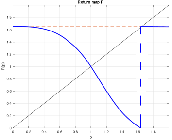
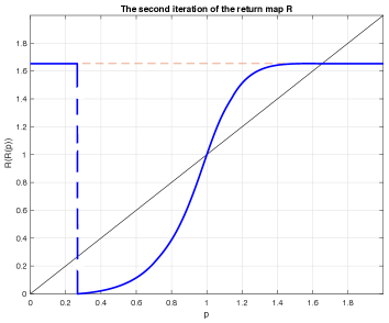
Figure 3: Return map ${\cal R}$ for equation (25) (on the left) and its second iteration ${\cal R}^{2}$ (on the right). The dashed horizontal line corresponds to ${\cal R}(0)$. Note that ${\cal R}^{2}$ and ${\cal R}$ share one point of discontinuity (not appreciable on the right frame).

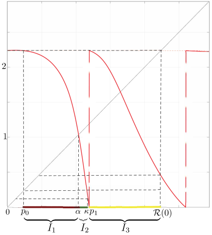
Figure 4: Graph of the return map ${\cal R}$ for equation (19) (discontinuous red solid curve). The upper dashed horizontal line corresponds to ${\cal R}(0)$. The closed subintervals $I_{1}$ (brown), $I_{2}$ (green), $I_{3}$ (yellow) of $K$ have pairwise disjoint interiors and satisfy the relations $I_{2}\cup I_{3}\subset{\cal R}(I_{1})$, $I_{1}\subset{\cal R}(I_{2})$ , $I_{2}\cup I_{3}\subset{\cal R}(I_{3})$.

3.2 Chaotic behavior in the Magomedov equation

The forcing term $f(t)$ in (25) is close to the function $g(t)=1-\sin t$. In fact, the replacement of $f(t)$ with $1-\sin t$ in (25) produces dynamically insignificant changes in the return map so that the modified system has the same simple dynamics. However, by adding the linear term $0.32u(t)$ to (25), the behavior of the solutions changes dramatically. Indeed, as we show below, equation (19) introduced in Example 19 exhibits chaotic behaviour.

In the Appendix, we prove the following result (see also Figure 4, which represents the return map ${\cal R}$ for (19)).

Theorem 28

The return map ${\cal R}:K\to K$ for (19) has exactly two points of discontinuity $p_{1}\approx 1.11$ and $p_{2}\approx 2.61$ on the interval $[0,p_{2}]\supset{\cal R}(K)$, where

$${\cal R}(p_{1})={\cal R}(p_{2})={\cal R}(0)\approx 2.23,\quad{\cal R}(p_{1}-)={\cal R}(p_{2}-)=0.$$

Furthermore, ${\cal R}$ is differentiable on $[0,1.316]\setminus\{p_{1}\}$ and has a unique critical point $p_{c}\approx 0.108$ on this interval, where it reaches its absolute maximum. Finally, ${\cal R}^{\prime}(p_{1}-)<{\cal R}^{\prime}(p_{1}+)$, ${\cal R}(p)>p$ for all $p\in[0,0.9]$ and ${\cal R}({\cal R}(0))<0.9$.

This theorem implies the existence of a leftmost fixed point $\alpha\in(0.9,p_{1})$ for ${\cal R}$. Let $p_{0}\in(0,p_{1})$ be defined by ${\cal R}(p_{0})={\cal R}(0)$ and let $\kappa\in(\alpha,p_{1})$ be sufficiently close to $p_{1}$ to satisfy ${\cal R}(\kappa)<p_{0}$. Consider the following closed subintervals of $K$ with pairwise disjoint interiors

$$I_{1}=[p_{0},\alpha],\quad I_{2}=[\alpha,\kappa],\quad I_{3}=[p_{1},{\cal R}(0)].$$

These intervals are shown in Figure 4. Clearly, the return map is continuous on each of these intervals and

$$I_{2}\cup I_{3}\subset{\cal R}(I_{1}),\quad I_{1}\subset{\cal R}(I_{2}),\quad I_{2}\cup I_{3}\subset{\cal R}(I_{3}).$$

Writing the inclusion $I_{1}\subset{\cal R}(I_{2})$ in the form $I_{2}\to I_{1}$, and similarly the others, we obtain the following directed Markov graph associated with the collection $I_{1},I_{2},I_{3}$:

The adjacency matrix ${\cal A}=\{a_{ij}\}$ of the graph is defined as follows: $a_{ij}=1$ if and only if there is an edge from vertex $I_{i}$ to vertex $I_{j}$; otherwise, $a_{ij}=0$. Thus:

$${\cal A}=\begin{bmatrix}0&1&1\\ 1&0&0\\ 0&1&1\end{bmatrix}.$$

Consider the space $\Omega_{\cal A}^{+}$ of all one-sided paths on the above Markov graph (for example, $\omega=(I_{3},I_{3},I_{2},I_{1},I_{2},I_{1},I_{3},\dots)$) provided with the metrisable topology of component-wise convergence. It is easy to realise that $\Omega_{\cal A}^{+}$ is a closed perfect subspace of the product space $\{I_{1},I_{2},I_{3}\}^{\mathbb{N}}$ so that it is a Cantor set. Let $\sigma:\Omega_{\cal A}^{+}\to\Omega_{\cal A}^{+}$ denote the one-sided shift defined by $\sigma(\{I_{n_{k}}\})=\{I_{n_{k+1}}\}$ (e.g. $\sigma(I_{3},I_{3},I_{2},I_{1},I_{2},I_{1},I_{3},\dots)=(I_{3},I_{2},I_{1},I_{2},I_{1},I_{3},\dots)$). Since all elements of the matrix ${\cal A}^{3}$ are positive (hence, the matrix $\cal A$ is transitive [22, Definition 1.9.6]), the dynamical system $\sigma:\Omega_{\cal A}^{+}\to\Omega_{\cal A}^{+}$ is topologically mixing and its periodic points are dense in $\Omega_{\cal A}^{+}$, see [22, Proposition 1.9.9]. Then, an application of Theorem 15.1.5, Corollaries 1.9.5, 15.1.6, 15.1.8, and Proposition 3.2.5 in [22] yields the following result (notice that the greatest eigenvalue of ${\cal A}$ is $\lambda_{{\cal A}}^{max}=(\sqrt{5}+1)/2$).

Theorem 29

There is a closed subset $J\subset I_{1}\cup I_{2}\cup I_{3}$ and a continuous surjection $h:J\to\Omega_{\cal A}^{+}$ such that ${\cal R}(J)\subset J$ and the following diagram is commutative

Moreover, to each periodic orbit $\omega\in\Omega_{\cal A}^{+}$ corresponds at least one periodic point of the same period in $h^{-1}(\omega)$ so that ${\cal R}:J\to J$ has an infinite set of periodic solutions. In fact, the number of different $n$-periodic orbits of $\cal R$ is bigger than or equal to the trace $Tr{\cal A}^{n}$, and the topological entropy of ${\cal R}:J\to J$ is at least $\log((\sqrt{5}+1)/2)>0$.

In this way, equation (19) has an infinite set of periodic solutions. In particular, Figure 4 shows that it has a $2\pi$-periodic solution $u_{1}$ with $\alpha=\max_{t\in{\mathbb{R}}}u_{1}(t)\approx 1.037,$ and a $4\pi$-periodic solution $u_{2}$ with $\gamma=\max_{t\in{\mathbb{R}}}u_{2}(t)\approx 1.65$. The graph of the second iteration ${\cal R}^{2}$ restricted to the interval $[\alpha,\gamma]$ suggests that ${\cal R}$ has an infinite set of unstable periodic solutions. In Figure 5, we represent two particular solutions of equation (19): the curve $(t,u(t))$ of the solution $u=u(t,1)$, $t<350$, and the projection of the solution $u=u(t,0)$ on the plane $(u(t),u(t-h))$.

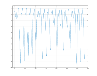
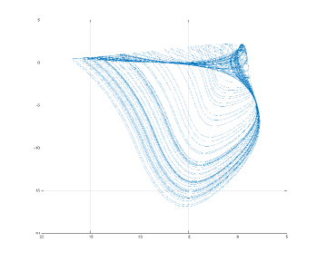
Figure 5: On the left, we represent the solution $u=u(t,1)$ of equation (19); on the right, the projection of the solution $u=u(t,0)$ of (19) on the plane $(u(t,0),u(t-h,0))$.

Appendix

Here, we present a proof of Theorem 28 based on the analysis of the explicit formulae for the solutions of the initial value problem

$$u^{\prime}(t)=au(t)-u(t-h)+1-\sin t,\ u(s)\equiv p=(1-\sin q)/d,\ s\in[q-h,q],$$ (26)

where $a=0.32$, $h=3\pi/2$, $d=0.68$ and $q\in[-0.5\pi,0.4]$ (note that, by Example 24, $\beta_{1}\approx 0.39289<0.4$). For our purposes, it suffices to integrate (26) on two steps: $[q,q+h]$ and $[q+h,q+2h]$. First, we observe that the unique periodic solution $p(t)$ of the ordinary differential equation $u^{\prime}(t)=au(t)+k\sin(t+\varphi)$ has the form

$$u(t)=-\frac{k}{\sqrt{a^{2}+1}}\sin(t+\varphi+\theta_{0}),\ \mbox{where}\ \theta_{0}:=\arcsin\frac{1}{\sqrt{a^{2}+1}}.$$

Thus, integrating (26) on $[q,q+h]$, we easily find that

$$u(t)=C_{0}\sin(t+\theta_{0})+C_{1}+C_{2}e^{a(t-q)},\ \mbox{where}\ C_{0}=\frac{1}{\sqrt{a^{2}+1}},\ C_{1}=\frac{p-1}{a},$$ (27)

$$C_{2}=p-C_{1}-C_{0}\sin(q+\theta_{0}).$$

Hence, solving (26) on $[q+h,q+2h]$ amounts to the integration of the linear inhomogeneous ordinary differential equation

$$u^{\prime}(t)=au(t)-(C_{0}\sin(t-h+\theta_{0})+C_{1}+C_{2}e^{a(t-h-q)})+1-\sin t,\$$ (28)

subject to the initial condition

$$u(q+h)=-C_{0}\cos(q+\theta_{0})+C_{1}+C_{2}e^{ah}=:C_{3}.$$ (29)

The solution of (28), (29) is given by

$$u(t)=C^{*}_{0}\cos(t+2\theta_{0})+C_{0}\sin(t+\theta_{0})+C^{*}_{1}-C_{2}(t-h-q)e^{a(t-h-q)}+C^{*}_{2}e^{a(t-h-q)},$$ (30)

where

$$\ C^{*}_{0}=\frac{1}{a^{2}+1},\ C^{*}_{1}=\frac{C_{1}-1}{a},\ C_{2}^{*}=C_{3}-C^{*}_{0}\sin(q+2\theta_{0})+C_{0}\cos(q+\theta_{0})-C^{*}_{1}.$$

This implies that the first derivative $u^{\prime}(t)$ is an analytic function of the variables $q\in[-0.5\pi,0.4]$ and $t\in[q+h,q+2h]$:

$$u^{\prime}(t)=-C^{*}_{0}\sin(t+2\theta_{0})+C_{0}\cos(t+\theta_{0})+\left[-C_{2}a(t-h-q)+(C^{*}_{2}a-C_{2})\right]e^{a(t-h-q)}.$$

Note also that

$$u(q+2h)-u(q+h)=-C^{*}_{0}\cos(q+2\theta_{0})-C_{0}\sin(q+\theta_{0})+C^{*}_{1}-C_{2}he^{ah}+C^{*}_{2}e^{ah}-C_{3}.$$

Lemma 30

For all $q\in[0.105,0.4]$, $t\in[q+h,q+2h]$, it holds that $u^{\prime}(t)>0$. Furthermore, $u(q+2h)-u(q+h)>0$ for all $q\in[-0.12,0.4]$.

Proof 21

It is convenient to introduce the new variable $s=t-q-h\in[0,h]=[0,1.5\pi]$. Then we have to evaluate the elementary function

$$\Psi(s,q)=C_{0}\sin(s+q+\theta_{0})+C^{*}_{0}\cos(s+q+2\theta_{0})+\left[-C_{2}as+(C^{*}_{2}a-C_{2})\right]e^{as}$$

on the rectangle $\Pi=[0,1.5\pi]\times[0.105,0.4]$. Since $\min\{\Psi(s,q),\ (s,q)\in\Pi\}=0.0086\dots$, the first assertion of the lemma is proved. Similarly, the second conclusion follows from the computation of $\min\{u(q+2h)-u(q+h),\ q\in[-0.12,0.4]\}\approx 0.02057.$

Since the inequality $u^{\prime}(q+h)>0$ guarantees that the only critical point of $u(t)$ on the interval $[q,q+h]$ is a minimum point and $[0,1.316]\subseteq[0,\tilde{f}(0.105)]$, we obtain the following result:

Corollary 31

For all $p\in[0,1.316]$, the solution $u(t,p)$ is $U$-shaped on the interval $(q,\nu^{*}(q))$ (see Figure 6). Moreover, $\mu(q)-q<3\pi$ so that ${\cal R}^{\prime}(p+)<0$ for all $p\in(\tilde{f}(q_{0}),1.316]$, where $q_{0}\approx 1.1845$ is computed in Example 24.

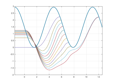
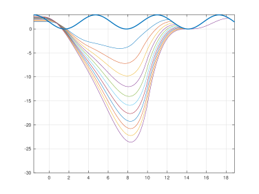
Figure 6: Graphs of solutions $u=u(t,p_{j})$ on $t\in[q_{j},\nu^{*}(q_{j})]$ together with the sine-like function $\tilde{f}$. On the left: $p_{j}=\tilde{f}(q_{j})=0.125\sqrt[4]{1000j},\ j=0,\dots,10$. On the right: $p_{j}=\tilde{f}(q_{j})=1+0.125\sqrt{15i},\ i=1,\dots 11.$

Lemma 32

The graph of $u(t,p)$ does not contain the point $(2.5\pi,0)$ and condition (M) is satisfied whenever $p\in{\cal I}=[1.26,2/0.68]$.

Proof 22

First, note that $u(t,p)=u(t),\ t\in[q,q+1.5\pi],$ for all $p\in{\cal I}$. In particular, $u(t)$ has a unique critical point (global minimum point) on the interval $(q,q+1.5\pi]$ so that $u(t)<0$ on $[\pi,q+1.5\pi]$ if $u(\pi)<0$ and $u(q+1.5\pi)=C_{3}<0$. It is easy to check that these inequalities hold for all $q\in[-0.5\pi,0.15]$.

Next, for all $t\in[q+1.5\pi,q+3\pi]$, we find that

$$u^{\prime}(t,p)=0.32u(t,p)-U(t,p)+1-\sin t\leq 0.32u(t,p)-u(t-h,p)+1-\sin t.$$

Thus a standard comparison argument shows that $u(t,p)\leq u(t)$, $t\in[q+1.5\pi,q+3\pi]$, where $u(t)$ is given by (30). Now, setting $s=t-q-h\in[0,h]=[0,1.5\pi]$, we present $u(t)$ as

$$\Phi(s,q)=C^{*}_{0}\sin(s+q+2\theta_{0})-C_{0}\cos(s+q+\theta_{0})+C^{*}_{1}+\left[-C_{2}s+C^{*}_{2}\right]e^{as}.$$

Then the inequality $u(t)<0,\ t\in[q+1.5\pi,2.5\pi],$ holds for all $q\in[-0.5\pi,0.15]$ if $\Phi(s,q)<0$ on the set $\Pi_{2}=\{(s,q):s+q\leq\pi,q\in[-0.5\pi,0.15],s\geq 0\}$. Now, we find that

$$\max\{\Phi(s,q),\ (s,q)\in\Pi_{2}\}=-0.0615\dots<0.$$

Thus $u(t,p)<0$ for all $t\in[\pi,2.5\pi]$ whenever $q\in[-0.5\pi,0.15]$. This proves the first assertion of the lemma. Finally, since ${\cal R}(p)>0$, condition (M) is satisfied for each $p\in[\tilde{f}(0.15),\tilde{f}(-\pi/2)]=[1.25\dots,2/0.68]$.

Now we are in a position to prove Theorem 28.

Proof 23 (of Theorem 28)

Since the computation of ${\cal R}(\bar{p})$ for each given $\bar{p}=\tilde{f}(\bar{q})\in K$ amounts to the explicit integration of some first order inhomogeneous linear differential equations with constant coefficients on a finite interval $[\bar{q},\nu^{*}(\bar{q})]$, and founding zeros of simple elementary functions on the same interval, we will assume that the value of ${\cal R}(\bar{p})$ can be found with the required accuracy. For example, the value of ${\cal R}(0)\approx 2.2$ can be found by solving the equation $u(t)=\tilde{f}(t)$ on the interval $[1.5\pi,2.5\pi]$, where $u(t)$ is given by (27). In a similar way, we can compute the value of ${\cal R}({\cal R}(0))\approx 0.45.$

Next, Corollary 31 and Remark 27 allow to apply Theorem 25 on the $q$-interval $(\alpha,\beta]=(0.105,0.5\pi]$. In order to prove that the associated $p$-interval $[\tilde{f}(\beta),\tilde{f}(\alpha))=[0,1.3\dots)$ contains one point $p_{1}$ of discontinuity, it suffices to take $q$ such that $\tilde{f}(q)=1.25$ and to check that $\nu^{*}(q)\in(3.5\pi,4.5\pi)$ (this $q$ corresponds to $q_{10}$ in the left frame of Figure 6). Invoking also Example 19, we establish all stated properties of ${\cal R}$ on the interval $[0,1.316]$. Concerning the computation of the approximate value of $p_{1}$, note that $p_{1}\in(a_{1},a_{2})\subset[0,1.316]$ if ${\cal R}(a_{1})<{\cal R}(a_{2})$ (particularly, we obtain immediately that $p_{1}\in(0.9,1.25)$ while a more accurate similar estimate implies that $p_{1}\approx 1.1$).

Finally, Lemma 32 shows that condition (M) is satisfied for all $p\in{\cal I}=[1.26,2/0.68]$. Then Theorem 15 and the proof of Corollary 20 imply that the restriction ${\cal R}:[p_{1},p_{2})\to K$ has continuous graph until the first eventual intersection of its closure with the real axis at some point $p_{2}$, where ${\cal R}(p_{2}-)=0,\ {\cal R}(p_{2})={\cal R}(0)>0$. In order to establish the existence of such $p_{2}$ and find its approximate value, it is enough to take $p^{*}_{i}=\tilde{f}(q_{i}^{*})=1+0.125\sqrt{15k}\in\{2.53\dots,2.60\dots\},$ with $k=10,11$, and to note that $\nu^{*}(q_{11}^{*})\in(5.5\pi,6.5\pi)$ while $\nu^{*}(q_{10}^{*})\in(3.5\pi,4.5\pi)$, see the right frame of Figure 6. In particular, this shows that $p_{2}>2.53>{\cal R}(0)$.

References

- [1] D. D. Bainov, S. Hristova, Differential Equations with Maxima, Chapman & Hall/CRC Pure and Applied Mathematics, 2011.
- [2] C.T.H. Baker, Development and application of Halanay-type theory: Evolutionary differential and difference equations with time lag, J. Comput. Appl. Math. 234 (2010), 2663–2682.
- [3] N. Bantsur, E. Trofimchuk, Existence and stability of the periodic and almost periodic solutions of quasilinear systems with maxima, Ukrainian Math. J. 50 (1998), 847–856.
- [4] P. Brunovský, A. Erdélyi, H.-O. Walther, On a model of a currency exchange rate - local stability and periodic solutions, J. Dyn. Differ. Equ. 16 (2004), 393–432.
- [5] I. Cojuharenco, D. Ryvkin, Peak-End rule versus average utility: How utility aggregation affects evaluations of experiences, J. Math. Psychol. 52 (2008), 326–335.
- [6] F. Y. Edgeworth, Mathematical Psychics: An Essay on the Application of Mathematics to the Moral Sciences (1881); reprinted (M. Kelly, New York, 1967).
- [7] A. Erdélyi, A delay differential equation model of oscillations of exchange rates, Ph.D. Thesis Bratislava, 2003.
- [8] T. Faria, E. Liz, J.J. Oliveira, S. Trofimchuk, On a generalized Yorke condition for scalar delayed population models, Discrete Contin. Dyn. Syst., Ser A 12 (2005), 481–500.
- [9] R. Franke, Reviving Kalecki’s business cycle model in a growth context, J. Econ. Dyn. Control 91 (2018), 157–171.
- [10] A. Ivanov, E. Liz, S. Trofimchuk, Halanay inequality, Yorke 3/2 stability criterion, and differential equations with maxima, Tohoku Math. J. 54 (2002), 277–295.
- [11] J. Gertner, The futile pursuit of happiness, The New York Times Magazine, (2003) https://www.nytimes.com/2003/09/07/magazine/the-futile-pursuit-of-happiness.html?smid=wa-share (last accessed June 2021).
- [12] D. Gilbert, Stumbling on Happiness. Knopf, New York, 2006.
- [13] A. Halanay, Differential Equations: Stability, Oscillations, Time Lags, Academic Press, New York and London, 1966.
- [14] J. K. Hale, Asymptotic Behavior of Dissipative Systems, Mathematical Surveys and Monographs 25, A.M.S., Providence, Rhode Island, 1988.
- [15] J. Hale, L. Magalhães, W. Oliva, An Introduction to Infinite Dynamical Systems–Geometric Theory, Springer-Verlag, New York, 1984.
- [16] J. K. Hale, S. M. Verduyn Lunel, Introduction to Functional Differential Equations, Applied Mathematical Sciences 99, Springer-Verlag, New York, 1993.
-
[17]
H. Huijer, Tracking happiness: My happiness review 2020,
https://www.trackinghappiness.com/happiness-diary-review-2020/ (last accessed June 2021). - [18] D. Kahneman, B. L. Fredrickson, Ch. A. Schreiber, D. A. Redelmeier, When more pain is preferred to less: adding a better end, Psychol. Sci. 4 (1993), 401–405.
- [19] D. Kahneman, P. P. Wakker, R. Sarin, Back to Bentham? Explorations of Experienced Utility, Q. J. Econ. 112 (1997), 375–405.
- [20] D. Kahneman, A.Tversky (Eds.), Choices, Values, and Frames, Cambridge University Press, Cambridge, 2000.
- [21] M. Kalecki, A macroeconomic theory of the business cycle, Econometrica 3 (1935), 327–344.
- [22] A. Katok, B. Hasselblatt, Introduction to the Modern Theory of Dynamical Systems, Encyclopedia of Mathematics and its Applications, vol. 54, Cambridge Univ. Press, Cambridge, 1995.
- [23] A. A. Keller, Time-Delay Systems: with Applications to Economic Dynamics and Control, LAP Lambert Academic Publishing, 2011.
- [24] T. Krisztin, On stability properties for one-dimensional functional differential equations, Funkc. Ekvacioj, Ser. Int. 34 (1991), 241–256 .
- [25] E. Liz, V. Tkachenko and S. Trofimchuk, A global stability criterion for scalar functional differential equations, SIAM J. Math. Anal. 35 (2003), 596–622.
- [26] E. Liz, V. Tkachenko, S. Trofimchuk, Yorke and Wright 3/2-stability theorems from a unified point of view, Discrete Contin. Dyn. Syst., suppl. (2003), 580–589.
- [27] A.R. Magomedov, Ordinary Differential Equations with Maxima (in Russian), Baku, Elm, 1991.
- [28] C. K. Morewedge, D. T. Gilbert, T. D. Wilson, The least likely of times: how remembering the past biases forecasts of the future, Psychol. Sci. 16 (2005), 626–630.
- [29] A.D. Myshkis, On certain problems in the theory of differential equations with deviating argument, Russ. Math. Surv. 32 (1977), 181–213.
- [30] A.D. Myshkis, Soviet Mathematicians: My Memories (In Russian), Editorial LKI, Moscow, 2007.
- [31] V. Petukhov, Questions about qualitative investigations of differential equations with “maxima”. Izv. Vyssh. Uchebn. Zaved. Mat. 3 (1964), 116–119 (In Russian).
- [32] M. Pinto, S. Trofimchuk, Stability and existence of multiple periodic solutions for a quasilinear differential equation with maxima, Proc. Roy. Soc. Edinburgh Sect. A 130 (2000), 1103–1118.
- [33] M. Rontó, A. Samoilenko, S. Trofimchuk, The theory of the numerical-analytic method: Achievements and new trends of development. III. Ukrainian Math. J. 50 (1998), 1091–1114.
- [34] A. Samoilenko, E. Trofimchuk, N. Bantsur, Periodic and almost periodic solutions of the systems of differential equations with maxima (in Ukrainian), Reports of the National Academy of Sciences of Ukraine 1 (1998), 47–52.
- [35] G.H. Sarafova, D.D. Bainov, Application of A. M. Samoilenko’s numerical-analytic method to the investigation of periodic linear differential equations with maxima. (Russian) Rev. Roumaine Sci. Tech. Ser. Mec. Appl. 26 (1981), 595–603.
- [36] J. Touboul, A. Romagnoni, R. Schwartz, On the dynamic interplay between positive and negative affects, Neural Comput. 29 (2017), 897–936.
- [37] H. Voulov, D. Bainov, On the asymptotic stability of differential equations with ‘maxima’. Rend. Circ. Mat. Palermo 40 (1991), 385–420.
- [38] Walther, H.-O. The impact on mathematics of the paper “Oscillation and Chaos in Physiological Control Systems”, by Mackey and Glass in Science, 1977. arXiv:2001.09010, (2020).
- [39] J. A. Yorke, Asymptotic stability for one dimensional differential-delay equations, J. Difffer. Equ. 7 (1970), 189–202.
- [40] P.J. Zak, Kaleckian lags in general equilibrium, Rev. Political Economy 11 (1999), 321–330.