TeV-scale Lepton Number Violation: Connecting Leptogenesis, Neutrinoless Double Beta Decay, and Colliders

Abstract

In the context of TeV-scale lepton number violating (LNV) interactions, we illustrate the interplay between leptogenesis, neutrinoless double beta ($0\nu\beta\beta$) decay, and LNV searches at proton-proton colliders. Using a concrete model for illustration, we identify the parameter space where standard thermal leptogenesis is rendered unviable due to washout processes and show how $0\nu\beta\beta$ decay and $pp$ collisions provide complementary probes. We find that the new particle spectrum can have a decisive impact on the relative sensitivity of these two probes.

1 Introduction

With the current knowledge of the Standard Model (SM) of particle physics, lepton number appears to be an accidentally conserved quantum number at the classical level. However, many beyond the Standard Model (BSM) scenarios contain lepton number violating (LNV) interactions. Consider, for instance, a minimal extension of the SM with right-handed neutrinos (RHN). A lepton-number conserving Dirac mass term would lead to massive neutrinos as required by neutrino oscillations. However, unless one explicitly requires lepton number conservation, one may also include a LNV RHN mass term. Diagonalization of the full mass matrix for the neutral leptons implies that that light neutrinos are also Majorana particles. For sufficiently heavy RHN, the Dirac mass Yukawa couplings may be as large as $\mathcal{O}(1)$ while accommodating the scale of light neutrino masses implied by neutrino oscillations and cosmological neutrino mass bounds. The light neutrino interactions then inherit the LNV properties of Majorana neutrinos as a consequence of this well-known see-saw neutrino mass mechanism.

At the same time, LNV interactions can play an important role in generating the baryon asymmetry of the Universe (BAU), which is usually quantified in terms of the baryon-to-photon number density based on the PLANCK 2018 data Zyla:2020zbs ; Aghanim:2018eyx

$$\eta_{B}^{\mathrm{obs}}=\frac{n_{B}}{n_{\gamma}}=(6.12\pm 0.04)\times 10^{-10}\,,$$ (1)

or the yield, normalized to the entropy density $s$,

$$Y_{B}^{\mathrm{obs}}=\frac{n_{B}}{s}=(8.71\pm 0.06)\times 10^{-11}\,.$$ (2)

As a key test of standard cosmology, this value is in agreement with limits coming from Big Bang Nucleosynthesis Zyla:2020zbs . According to the established three Sakharov conditions Sakharov:1967dj , a mechanism explaining the BAU needs to include (i) baryon number (B-) violation, (ii) C- and CP-violation and (iii) an out-of-equilibrium condition (or CPT-violation). As these conditions are not sufficiently satisfied within the SM, the observed BAU clearly requires BSM physics. Due to the SM ($B+L$) violating electroweak sphalerons being active above the electroweak scale, one possibility is to generate first a lepton asymmetry which then gets translated into a baryon asymmetry (baryogenesis via leptogenesis) Fukugita:1986hr . Hence, the observation of LNV interactions can have far-reaching consequences. It could not only give indications on a Majorana contribution to neutrino masses but also have implications for the validity of different leptogenesis scenarios.

If LNV interactions exist in nature, then it is natural to explore the possible associated mass scale, $\Lambda$. In context of standard thermal leptogenesis and the simplest scenario with RHNs, consistency with light neutrino phenomenology implies $\Lambda>10^{9}$ GeV Davidson:2002qv . Direct experimental access to new particles and LNV interactions at these scales is clearly unfeasible, though indirect indications could be seen via searches for neutrinoless double beta ($0\nu\beta\beta$) decay. Searches to date have yielded null results, with the present strongest limit on the half-life of ¹³⁶Xe having been set by the KamLAND-Zen experiment KamLAND-Zen:2016pfg

$$T^{0\nu\beta\beta}_{1/2}>1.07\times 10^{26}~{}\textrm{years at 90\% C.L.}\,$$ (3)

The next generation of “tonne-scale” $0\nu\beta\beta$ decay searches aim to increase this sensitivity by two orders of magnitude, with a variety of isotopes under consideration Albert:2017hjq ; Kharusi:2018eqi ; Abgrall:2017syy ; Armengaud:2019loe ; CUPIDInterestGroup:2019inu ; Paton:2019kgy . Should the three light neutrinos have Majorana masses and an inverted mass hierarchy spectrum, then the ton scale searches would expect to observe a signal. In the “standard mechanism”, wherein the underlying process involves the exchange of three light Majorana neutrinos, the observation of a signal would point to a high scale for $\Lambda$ associated with standard thermal leptogenesis and the conventional seesaw mechanism.

In the absence of further experimental information, it is interesting to ask whether LNV interactions may live at multiple scales, including not only the high scale required by standard thermal leptogenesis but also at lower scales. In this work, we investigate the possibility that additional LNV interactions may exist with the associated $\Lambda$ as low as $\mathcal{O}(\mathrm{TeV})$. LNV interactions at this scale could contribute directly to $0\nu\beta\beta$ decay at an observable level, regardless of the contribution from the light neutrino spectrum. In fact, discovery of LNV in $0\nu\beta\beta$ decay would not yield information about the underlying mechanism. On the other hand, observation of an LNV signal in high energy proton-proton collisions, such as pairs of same sign leptons and an associated di-jet pair, would point to LNV at the TeV scale. One would naturally wonder about the resulting implications for leptogenesis.

In this work we explore these implications in detail using a concrete, simplified model for illustration. Our study builds on earlier analyses that addressed this question in an effective field theory (EFT) context Deppisch:2015yqa ; Deppisch:2017ecm ; Li:2019fhz ; Deppisch:2020oyx . For sufficiently heavy $\Lambda$, one may integrate the new degrees of freedom, yielding a set of non-renormalizable LNV interactions built from SM fields only. These operators have odd mass dimension $d$, starting with the well-known “Weinberg operator” ($d=5$) that gives rise to light neutrino Majorana masses. For surveys of LNV effective operators up to $d=11$, see, e.g. Refs. Babu:2001ex ; deGouvea:2007qla ; Deppisch:2017ecm . Importantly, the EFT analyses imply that in the context of TeV scale LNV, observation of a signal in either $0\nu\beta\beta$ decay and/or $pp$ collisions could be fatal for the viability of standard thermal leptogenesis. The reason is that the observation of LNV interactions based on higher dimensional operators would imply a strong washout of a pre-existing lepton-asymmetry that was potentially generated at a high scale.

EFT analyses, however, are limited in their validity and lack information of concrete values for couplings and masses of the new physics (NP) involved. Hence, we confront in this work the previous EFT results with a simplified model. Doing so allows us to investigate in detail the interplay of leptogenesis with LNV searches. We include the new interactions explicitly in the leptogenesis Boltzmann equations, allowing us to analyze in detail the dependence of the BAU on the masses and couplings associated with the new particles and their interactions. From the Boltzmann equation solutions, we identify the regions of the model mass and coupling parameter space for which the TeV scale LNV interactions would render unviable standard thermal leptogenesis (assuming also the presence of the heavy RHN as described above). We then utilize state-of-the-art hadronic and nuclear physics methods relevant to $0\nu\beta\beta$ decay and machine learning techniques for collider LNV searches to delineate the sensitivity of these probes to the leptogenesis unviable parameter space. In the context of our illustrative model, we find that

• The observation of an LNV signal at the Large Hadron Collider (LHC) and/or a future 100 TeV $pp$ collider would preclude the viability of standard thermal leptogenesis.

• The observation of $0\nu\beta\beta$ decay could also rule out the standard leptogenesis paradigm, assuming the $0\nu\beta\beta$ decay amplitude is dominated by the TeV scale LNV mechanism. Additional information, such as the results from $pp$ collider LNV searches, knowledge of the light neutrino mass hierarchy, and/or the sum of light neutrino masses would be needed identify the underlying $0\nu\beta\beta$ decay mechanism.

• The relative reaches of $0\nu\beta\beta$ decay and collider LNV searches depends decisively on the new particle spectrum — a feature not readily seen within the previously used pure EFT approach.

• The observation of experimental signature would be consistent with the scale of light neutrino masses implied by neutrino oscillation experiments as well as cosmological and astrophysical neutrino mass probes.

The outcome of our analysis leading to these conclusions is organized as follows: In Section 2, we first introduce the simplified model set-up that we used for our study. Then, we introduce the Boltzmann-equation framework and the consequences with respect to leptogenesis in Section 3. In Section 4, we discuss the performed collider analysis and in Section 5 the treatment with respect to $0\nu\beta\beta$ decay. In Section 6, we present our results and conclude in Section 7.

2 A simplified model for TeV-scale LNV

For the standard leptogenesis scenario Fukugita:1986hr , at least two heavy right-handed neutrinos $N_{j}$ are needed to generate a CP-asymmetry via the one-loop decay of the lightest right-handed neutrino Nanopoulos:1979gx ; Kolb:1979qa . We consider the broadly studied situation Davidson:2008bu ; Buchmuller:2004nz ; Giudice:2003jh where the lepton asymmetry is produced in a single flavor, the neutrino masses are hierarchical ($M_{1}\ll M_{2},M_{3}$), and the decays of the two heavier neutrinos ($N_{2}$ and $N_{3}$) are neglected. Henceforth, we will refer to the lightest neutrino $N_{1}$ simply as $N$, dropping the flavor subscript. The interaction part of the Lagrangian is given by:

$$\mathscr{L}=y_{N}\,\overline{L}(i\tau^{2})H^{\ast}N-\frac{m_{N}}{2}\overline{N^{c}}N+\mathrm{h.c.}\ ,$$ (4)

where $L=(\nu_{e},e)_{L}$ and $\tau$’s are the Pauli matrices in isospace. While assuming that a lepton-asymmetry might have been generated via the decay of right-handed neutrinos at a high scale, we want to investigate the impact of additional LNV interactions at the TeV scale. For these purposes, we introduce a simplified model set-up that represents a possible realisation of the dim-9 effective operator studied in Prezeau:2003xn ; Deppisch:2015yqa ; Graesser:2016bpz as we will discuss in more detail later. The model includes a scalar $S$ transforming as $(1,2,1)$ under $SU(3)_{C}\times SU(2)_{L}\times U(1)_{Y}$ and a Majorana fermion $F$ that transforms as an SM gauge singlet. Note, we use the convention $Y=Q_{\mathit{EM}}-T_{3}$. The Lagrangian reads

$$\widetilde{\mathscr{L}}=g_{Q}\,\overline{Q}Sd_{R}+g_{L}\,\overline{L}(i\tau^{2})S^{\ast}F-m_{S}^{2}\,S^{\dagger}S-\frac{m_{F}}{2}\,\overline{F^{c}}F+\lambda_{HS}\,(S^{\dagger}H)^{2}+...\ ,$$ (5)

where $Q=(u_{L},d_{L})$ and $q_{R}=(u_{R},d_{R})$ are the left-handed and right-handed quark isospinors, respectively. The ellipsis indicates other possible terms such as $SH^{3}$ and $S^{3}H$. For simplicity, we omit those terms and also assume that the heavy neutrino $N$ will not interact with the new fields introduced.

Besides the generation of small Majorana neutrino masses via the see-saw mechanism Minkowski:1977sc ; Yanagida:1980xy ; Glashow:1979nm ; GellMann:1980vs ; Mohapatra:1980yp induced by the right-handed neutrino $N$, additional contributions can be generated at one-loop level via the interactions in the Lagrangian (5), as shown in Fig. 1. The magnitude of the contribution to the neutrino mass matrix is controlled by the coupling $\lambda_{HS}$ and can be estimated as

$$m_{\nu}\sim\dfrac{\lambda_{HS}}{\Lambda}\dfrac{\left(g_{L}\,\langle H\rangle\right)^{2}}{16\pi^{2}}\ .$$ (6)

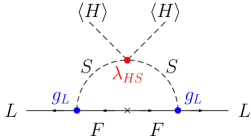
Figure 1: One-loop contribution to the Weinberg operator Weinberg:1979sa induced by the interactions in Eq. 5. Note that the magnitude of this contribution is proportional to the coupling $\lambda_{HS}$ that does not enter the amplitudes for $0\nu\beta\beta$-decay or same-sign dilepton plus di-jet production in $pp$ collisions.

For low energy $0\nu\beta\beta$-decay process, the heavy particles in the Lagrangian (5) can be integrated out, yielding the effective dimension-nine LNV interaction:

$$\mathscr{L}_{\mathit{LNV}}^{\mathrm{eff}}=\frac{C_{1}}{\Lambda^{5}}\mathcal{O}_{1}+\mathrm{h.c.}\ ,\quad\mathcal{O}_{1}=\bar{Q}\tau^{+}d\bar{Q}\tau^{+}d\bar{L}L^{c}\,.$$ (7)

We can match

$$C_{1}=g_{L}^{2}\,g_{Q}^{2}\quad\mathrm{and}\quad\Lambda^{5}=m_{S}^{4}\,m_{F}\ .$$ (8)

Interestingly, this demonstrates that TeV-scale masses for $m_{S}$ and $m_{F}$ are not in conflict with constraints from neutrino masses, (6), as in such a model realisation the contribution to ${0\nu\beta\beta}$-decay (depending on $g_{L},g_{Q}$ only) is independent from lowest order contribution to the neutrino mass (depending on $\lambda_{HS}$). In the following, we will study the impact of the new interactions in (5) on the baryon asymmetry generated from the heavy-right handed neutrinos and their detection possibilities at colliders and ${0\nu\beta\beta}$-decay experiments.

Figure 2: The realization of the $0\nu\beta\beta$-decay dim-9 operator induced by the interactions in Eq. 5. The scalar $S$ transforms as $(1,2,1)$ under $SU(3)_{C}\times SU(2)_{L}\times U(1)_{Y}$, and the Majorana fermion $F$ transforms as an SM gauge singlet.

3 Leptogenesis

One of the most popular explanations for the observed baryon asymmetry is baryogenesis via leptogenesis Fukugita:1986hr . In this mechanism, a lepton asymmetry is generated via the $B-L$ violating decays of right-handed heavy neutrinos. Due to the interference of the tree-level and one-loop contribution to the decays and the presence of at least two right-handed neutrinos, a net $CP$-asymmetry can occur. When the decays fall out of equilibrium during the cooling of the Universe, a final lepton asymmetry is generated. If this happens before the electroweak phase transition, the Standard Model electroweak sphaleron processes can transfer this lepton asymmetry into a baryon asymmetry. In the standard leptogenesis scenario, the same interactions that induce the right-handed neutrino decays, cause also $\Delta L=1$ and $\Delta L=2$ scattering processes that can destroy again this asymmetry, the so-called “washout” processes. If the latter are too strong, the generated asymmetry can be again destroyed. In Deppisch:2013jxa , it was shown that the observation of a generic $\Delta L=2$ lepton number violating signal at the LHC or in ${0\nu\beta\beta}$-decay experiments (via an operator of dimension seven or higher), would directly imply a significant washout rate and hence would render the asymmetry generation insufficient Deppisch:2015yqa ; Deppisch:2017ecm . While this interplay has been previously described in an effective field theory approach only, we want to investigate this within our simplified model set-up as described in Section 2. To this end, we analyze the potential to generate the observed baryon asymmetry within our simplified model which consists out of the SM extended by a right-handed neutrino (standard leptogenesis scenario) and an additional new physics contribution as defined in Eq. (5) leading to additional LNV washout processes experimentally accessible at the TeV scale.

First, we classify and study the relevant processes that will have an impact on the predicted baryon asymmetry. Hereby, we indicate the contributions that arise from Eq. (5), with a tilde ( $\widetilde{}$ ) and the contributions arising from the standard thermal leptogenesis Lagrangian, Eq. (4), without any additional marker (see Fig. 3):

• Decays and inverse decays ($\Delta L=1$):

  $$D \equiv[N\leftrightarrow H^{\pm}L^{\mp}]\,.$$ (9)

  $$\widetilde{D} \equiv[F\leftrightarrow S^{\pm}L^{\mp}]\,.$$ (10)

• Scattering processes ($\Delta L=1$), with the subscript indicating exchange via $s$- or $t$-channel:

  $$S_{s} =[LN\leftrightarrow U_{3}D_{3}]\quad,\qquad 2S_{t}=[N\bar{U}_{3}\leftrightarrow D_{3}\bar{L}]+[N\bar{D}_{3}\leftrightarrow U_{3}\bar{L}]\,.$$ (11)

  $$\widetilde{S}_{s} =[LF\leftrightarrow U_{1}D_{1}]\quad,\qquad 2\widetilde{S}_{t}=[F\bar{U}_{1}\leftrightarrow D_{1}\bar{L}]+[F\bar{D}_{1}\leftrightarrow U_{1}\bar{L}]\,.$$ (12)

• Scattering processes ($\Delta L=2$) with the Majorana fermion $F$ as mediator:

  $$N_{s} \equiv[LH\leftrightarrow\bar{L}\bar{H}]\qquad\textrm{and}\qquad N_{t}\equiv[LL\leftrightarrow\bar{H}\bar{H}]\,.$$ (13)

  $$\widetilde{N}_{s} \equiv[LS\leftrightarrow\bar{L}\bar{S}]\qquad\textrm{and}\qquad\widetilde{N}_{t}\equiv[LL\leftrightarrow\bar{S}\bar{S}]\,.$$ (14)

(a) $\widetilde{S}_{s}$ with $\Delta L=1$

(b) $\widetilde{S}_{t}$ with $\Delta L=1$

(c) $\widetilde{S}_{t}$ with $\Delta L=1$

(d) $\widetilde{N}_{s}$ with $\Delta L=2$

(e) $\widetilde{N}_{s}$ with $\Delta L=2$

(f) $\widetilde{N}_{t}$ with $\Delta L=2$

Figure 3: Relevant lepton-number violating processes arising from our extended Lagrangian that contribute to the washout additionally to the usual washout processes which occur within the standard leptogenesis scenario including right-handed neutrinos.

Hereby, the subscript $s$($t$) depicts a corresponding $s$($t$)-channel exchange as indicated in Fig. 3. In our analysis we generally neglect scattering processes with gauge bosons in order to avoid an unphysical logarithmic enhancement of $g^{2}\ln(gT/m_{N})$ that would not occur in a full thermal calculation at NLO. In principle, IR divergences would arise for a soft gauge boson. If regularized with a thermal mass, a logarithmic dependence ($g^{2}\ln(gT/m_{N})$) would remain. As was demonstrated in Salvio:2011sf for the standard leptogenesis scenario with right-handed neutrinos, this logarithmic dependence would cancel, when including the corresponding thermal distribution of the gauge bosons in a thermal plasma. This cancellation would, for instance, naturally occur in a calculation using the Closed Time Path formalism Garbrecht:2018mrp . As the scattering processes can be generally seen as higher-order correction to the corresponding decays, it was recommended by Salvio:2011sf not to take these problematic processes into account, as a regularization with a thermal mass would lead to bigger uncertainties than when directly neglecting those. As a similar behaviour is expected for the gauge scattering in our extended model (the dominant washout contribution arises from the inverse decay as will be discussed later in more detail), we neglect these processes also in our washout calculation. Following the same argumentation, we also neglect the scattering with light quarks that would give rise to IR divergences in the standard leptogenesis scenario. As IR divergences do not appear in the quark scattering in our extended model set-up due to the massive scalar $S$ in the propagator (cp. Fig. 3 (a)-(c)), we systematically include these scattering processes in our washout calculation.

For describing the evolution of the lepton asymmetry we include all the outlined processes, Eqs. (9)-(14) and derive the Boltzmann equations for the yield of the right-handed neutrino $Y_{N}=n_{N}/s$ and the ($B-L$) asymmetry $Y_{{B-L}}$. For example, for the evolution of $Y_{N}$, we can write

$$zHs\frac{dY_{N}}{dz}=-\sum_{a,i,j}[Na\leftrightarrow ij]\,,$$ (15)

with $z=m_{N0}/T$ being the dimensionless time parameter, $m_{N0}$ is the zero-temperature mass, and $s$ the entropy density. Hereby, $[Na\leftrightarrow ij]$ comprises all relevant processes and permutations:

$$[Na\leftrightarrow ij] = \left[\dfrac{n_{N}n_{a}}{n_{N}^{\mathrm{(eq)}}n_{a}^{\mathrm{(eq)}}}-\dfrac{n_{i}n_{j}}{n_{i}^{\mathrm{(eq)}}n_{j}^{\mathrm{(eq)}}}\right]\gamma^{\mathrm{(eq)}}(ij\leftrightarrow Na)\,,$$ (16)

with $\gamma^{\mathrm{(eq)}}(ij\leftrightarrow Na)$ indicating the corresponding equilibrium reaction rates. In the derivation, we neglected Pauli blocking or Bose enhancement, which is to a good accuracy valid ($\langle E\rangle\approx 3T$ such that $(1\pm f)\approx 1$ Strumia:2006qk ). The expression for the $2-2$ scattering processes is given by

$$\gamma^{\mathrm{(eq)}}_{S}(ij\leftrightarrow ab)=\dfrac{T}{64\pi^{4}}\int_{s_{\min}}^{\infty}ds\ \sqrt{s}\,\hat{\sigma}(s)\,K_{1}\left(\dfrac{\sqrt{s}}{T}\right)\,,$$ (17)

with the reduced cross section $\hat{\sigma}\equiv 2s\,\lambda[1,m_{i}^{2}/s,m_{j}^{2}/s]\,\sigma$. Hereby, $\sigma$ is the total cross section summed over initial and final states, $\lambda[a,b,c]$ the Källen function, and $s$ the square of the centre-of-mass energy. The corresponding relation for decays reduces to

$$\gamma^{\mathrm{(eq)}}_{D}(N\leftrightarrow ij\cdots)=n_{N}^{\mathrm{(eq)}}\dfrac{K_{1}(z)}{K_{2}(z)}\Gamma_{N}\qquad\textrm{with}\quad n_{N}^{\mathrm{(eq)}}=\dfrac{3\zeta(3)g_{N}T^{3}}{8\pi^{2}}z^{2}K_{2}(z)\,,$$ (18)

with $n_{N}^{\mathrm{(eq)}}$ being the equilibrium number density, $\Gamma_{N}$ the decay width, and $g_{N}=2$ the number of degrees of freedom. Collecting all relevant processes that change the abundance of the neutrino, $Y_{N}$, and the one of the ($B-L$)-asymmetry, $Y_{B-L}$, we finally arrive at two coupled Boltzmann equations

$$\dfrac{dY_{N}}{dz} = -(D+S)\Big{(}Y_{N}-Y_{N}^{\mathrm{(eq)}}\Big{)}$$ (19)

$$\dfrac{dY_{B-L}}{dz} = -\epsilon\,D\,\Big{(}Y_{N}-Y_{N}^{\mathrm{(eq)}}\Big{)}-W^{\mathrm{tot}}\,Y_{B-L}\,.$$ (20)

We assume that all SM particles are in thermal equilibrium at all time. Due to its fast gauge interactions, we can assume equilibrium also for the new, heavy particle $S$. The new particle $F$, however, is not strictly in equilibrium during all of the relevant time, but we have checked that the assumption of equilibrium will not affect the evolution of $Y_{{B-L}}$, while having a significant advantage with respect to the computing time. Furthermore, $D,~{}W$ and $S$ indicate the relevant (inverse) decay, washout and scattering processes including both, the usual standard leptogenesis interactions as well as the ones arising from our new Lagrangian. We define the usual washout parameter $K$ as

$$K=\frac{\Gamma_{N}}{H(z=1)}\,.$$ (21)

In the following, we will study both, the strong ($K=10^{2}$) and weak ($K=10^{-2}$) washout scenario. As the new contribution in our model, Eq. (5) is not directly interacting with the sterile neutrino sector, the Boltzmann equation for the change of the heavy neutrino number density remains unaltered with respect to the standard leptogenesis case. The decay rate $D$ is given by

$$D(z)=\dfrac{\gamma_{D}}{zH(z)n_{N}^{\mathrm{(eq)}}}=\dfrac{1}{zH(z)}\dfrac{\,K_{1}(z)}{K_{2}(z)}\Gamma_{D}\,,$$ (22)

with $H(z)=1.66(\sqrt{g_{*}}m^{2}_{N0})/(M_{\mathrm{Pl}}\,z^{2})$ and $K_{n}(z)$ being the modified Bessel function of the second kind. The scattering rates, $S=2S_{s}+4S_{t}$, in Eq. (19) are given as

$$S_{s/t}(z)=\dfrac{\gamma_{S_{s/t}}}{zH(z)n_{N}^{\mathrm{(eq)}}}=\dfrac{1}{zH(z)}\dfrac{m_{N}}{48\pi^{2}\zeta(3)K_{2}(z)}I_{S_{s/t}}(z)\,,$$ (23)

with

$$I_{\{S_{s/t},N\}}(z)=\int_{x_{\min}}^{\infty}dx\ \sqrt{x}\,\hat{\sigma}_{\{S_{s/t},N\}}(x)\,K_{1}(\sqrt{x}\,z)\,.$$ (24)

For the simplification of some expressions, we have introduced the parameter $x=s/m_{N}^{2}$. In these expressions, $m_{N}$ differs from $m_{N0}$ because it will have a $T$-dependent component when thermal effects are included.

In contrast, the Boltzmann equation describing the $Y_{B-L}$-asymmetry evolution has to be adjusted to incorporate the new processes involved. However, as we do not assume any other $CP$ violating source than the heavy neutrino decay, the decay rate $D$ in the $Y_{B-L}$ Boltzmann evolution remains unaltered. However, for the washout we have to consider both, the standard washout contributions and our new interactions such that we adjust the washout term $W$ as follows

$$W^{\mathrm{tot}}(z)=W(z,Y_{N})+\widetilde{W}(z)\,.$$ (25)

The contribution $W(z,Y_{N})$ corresponds to the expression of the standard case

$$W(z,Y_{N})=2\Big{[}N(z)+S_{t}(z)\Big{]}\left(\dfrac{Y_{N}^{\mathrm{(eq)}}}{Y_{B-L}^{\mathrm{(eq)}}}\right)+S_{s}(z)\left(\dfrac{Y_{N}}{Y_{B-L}^{\mathrm{(eq)}}}\right)\,,$$ (26)

with the $\Delta L=1$ scattering rates $S_{s/t}$ as defined in Eqs. (23) (24), and the $\Delta L=2$ scattering $N(z)=N_{s}(z)+N_{t}(z)$ given as

$$N(z)=\dfrac{\gamma_{N}}{zH(z)n_{N}^{\mathrm{(eq)}}}=\dfrac{1}{zH(z)}\dfrac{m_{N}}{48\pi^{2}\zeta(3)K_{2}(z)}I_{N}(z)\,,$$ (27)

with the integral $I_{N}(z)$ stated in Eq. (24). Note that the inclusion of real intermediate states (RIS) in the $N_{s}$ scattering can lead to double counting with respect to the decays of the heavy right-handed neutrinos. Hence, as suggested in Salvio:2011sf , we do not include the decay term in the washout contribution in order to prevent for double counting. The new contributions to the washout can be expressed as

$$\widetilde{W}(z)=\left[\frac{1}{2}\widetilde{D}(z)+2\widetilde{N}(z)+2\widetilde{S}_{t}(z)+\widetilde{S}_{s}(z)\right]\left(\dfrac{Y_{N}^{\mathrm{(eq)}}}{Y_{B-L}^{\mathrm{(eq)}}}\right)\,,$$ (28)

where the decay rate of the heavy particles $F$ or $S$, depending on their mass hierarchy, is given by

$$\widetilde{D}(z)=\dfrac{\gamma_{\widetilde{D}}}{zH(z)n_{N}^{\mathrm{(eq)}}}=\dfrac{1}{zH(z)}f_{F,S}\left(\dfrac{m_{F,S}}{m_{N}}\right)^{2}\dfrac{\,K_{1}(z\,m_{F,S}/m_{N})}{K_{2}(z)}\Gamma_{F,S}\,.$$ (29)

Comparing with the decay rate of the heavy neutrino in Eq. (22) and the interaction rate in Eq. (18), we have to perform small adjustments. First, we rescaled the argument of the Bessel function by $(m_{F,S}/m_{N})$. Secondly, we accounted for the equilibrium number density of $F$ or $S$ in $\gamma_{\widetilde{D}}$. Due to the following relation of the equilibrium number densities

$$n_{F}^{\mathrm{(eq)}}(z) = n_{N}^{\mathrm{(eq)}}(z)\,\left(\dfrac{m_{F}}{m_{N}}\right)^{2}\dfrac{K_{2}(z\,m_{F}/m_{N})}{K_{2}(z)}\,,$$

$$n_{S}^{\mathrm{(eq)}}(z) = n_{N}^{\mathrm{(eq)}}(z)\,\dfrac{2}{3}\left(\dfrac{m_{S}}{m_{N}}\right)^{2}\dfrac{K_{2}(z\,m_{S}/m_{N})}{K_{2}(z)}\,,$$

we have to rescale our expression by $f_{F,S}(m_{F,S}/m_{N})^{2}$ with $f_{F}=1$ or $f_{S}=2/3$ due to the different number of degrees of freedom of $F,S$ with respect to $N$. Similarly, we can proceed with the scattering rates in Eqs. (23) and (27) to adjust for the new physics contributions,

$$\widetilde{S}_{s/t}(z)=\dfrac{\gamma_{\widetilde{S}_{s/t}}}{zH(z)n_{N}^{\mathrm{(eq)}}}=\dfrac{1}{zH(z)}\dfrac{m_{N}}{48\pi^{2}\zeta(3)K_{2}(z)}\left(\dfrac{m_{F}}{m_{N}}\right)^{3}I_{\widetilde{S}_{s/t}}(z)\,,$$ (30)

$$\widetilde{N}(z)=\dfrac{\gamma_{\widetilde{N}}}{zH(z)n_{N}^{\mathrm{(eq)}}}=\dfrac{1}{zH(z)}\dfrac{m_{N}}{48\pi^{2}\zeta(3)K_{2}(z)}\left(\dfrac{m_{F}}{m_{N}}\right)^{3}I_{\widetilde{N}}(z)\,,$$ (31)

with

$$I_{\{\widetilde{S}_{s/t},\widetilde{N}\}}(z)=\int_{y_{\min}}^{\infty}dy\ \sqrt{y}\,\hat{\sigma}_{\{\widetilde{S}_{s/t},\widetilde{N}\}}(y)\,K_{1}(\sqrt{y}\,z\,m_{F}/m_{N})\,.$$ (32)

For convenience we have defined $y=\sqrt{s}/m_{F}^{2}$. Note that in contrast to the standard leptogenesis scenario, we do not include the RIS subtraction in this case, as in the relevant regime (until the lepton asymmetry is wiped out below the experimental value), the hierarchy $m_{S}>m_{F}$ always holds (see Fig. 4). Hence, no double counting occurs as the contribution $\widetilde{D}$ in Eq. 28 includes only the inverse decays $FL\rightarrow S$ and not $SL\rightarrow F$. Only the latter one would lead to a double counting as it is already accounted for in the scattering processes $\widetilde{N}_{s}$ when the $F$ in the propagator is produced resonantly (cp. Fig. 3 (d)). As we will later show, before $z=10^{6}$, $\widetilde{W}$ is dominated by the contribution $\widetilde{D}$. Therefore, we approximate the new washout only by the inverse decays for later times (concretely, $z>100$) such that no RIS subtraction needs to be included. This approximation eases the numerical solution of the Boltzmann equation up to the electroweak scale, leading to a conservative limit of the washout and hence on the viable parameter space.

In our set-up, we consider a heavy neutrino with $m_{N0}=10^{10}~{}\mathrm{GeV}$ around which scale the generation of the asymmetry takes place roughly. As at such high temperatures, masses can receive sizeable thermal corrections, which could even lead to an altered mass hierarchy with respect to $T=0$. Hence, we consider thermal masses in our evolution of the neutrino and lepton number density:

$$m_{N}^{2}(T) =m^{2}_{N0}+\frac{1}{8}y^{2}_{N}T^{2}$$ (33)

$$m_{F}^{2}(T) =m^{2}_{F0}+\frac{1}{8}g^{2}_{L}T^{2}$$ (34)

$$m_{S}^{2}(T) =m^{2}_{S0}+\left[\frac{3}{16}g_{2}^{2}+\frac{1}{16}g_{Y}^{2}+\frac{3}{12}g_{Q}^{2}+\frac{1}{12}g_{L}^{2}\right]T^{2}$$ (35)

$$m_{H}^{2}(T) =\left[\frac{3}{16}g_{2}^{2}+\frac{1}{16}g_{Y}^{2}+\frac{1}{4}y_{t}^{2}+\frac{1}{2}\lambda_{H}\right]T^{2}$$ (36)

$$m_{Q}^{2}(T) =\left[\frac{1}{6}g_{3}^{2}+\frac{3}{32}g_{2}^{2}+\frac{1}{288}g_{Y}^{2}+\frac{1}{16}y_{t}^{2}+\frac{1}{16}g_{Q}^{2}\right]T^{2}$$ (37)

$$m_{u}^{2}(T) =\left[\frac{1}{6}g_{3}^{2}+\frac{1}{18}g_{Y}^{2}+\frac{1}{8}y_{t}^{2}\right]T^{2}$$ (38)

$$m_{d}^{2}(T) =\left[\frac{1}{6}g_{3}^{2}+\frac{1}{72}g_{Y}^{2}+\frac{1}{8}y_{b}^{2}+\frac{1}{8}g_{Q}^{2}\right]T^{2}$$ (39)

$$m_{L}^{2}(T) =\left[\frac{3}{32}g_{2}^{2}+\frac{1}{32}g_{Y}^{2}+\frac{1}{16}g_{L}^{2}\right]T^{2}\,,$$ (40)

where we can express $T$ as $T=m_{N0}/z$. The definitions of $m_{F0}$ and $m_{S0}$ are analogous to $m_{N0}$. Here, we neglect contributions from the right-handed neutrino to the standard model masses, as those will only become relevant for $T>m_{N}$. In this regime, however, contributions are negligible with respect to the ones originating from the SM itself due to a comparably small coupling ($y^{\mathrm{strong}}_{N}=0.02$, $y^{\mathrm{weak}}_{N}=0.0002$). Hence they can be safely neglected. We show the evolution of the thermal masses in Fig. 4, where we have chosen $K=10^{2}$ such that $y_{N}=0.02$ and $g_{L}=g_{Q}=10^{-2}$. Relative to the heavy neutrino mass at zero temperature, the thermal corrections have almost no impact on $m_{N}(T)$, except for $z>10^{-2}$. This is in contrast to the evolution of the other particle masses. For instance, even when choosing at zero temperature $m_{F0}>m_{S0}$, the thermal corrections grow faster for $S$ than $F$ such that in the relevant temperature regime, the hierarchy of the particles changes (e.g. at $z=1$, $m_{S}>m_{F}$). Another interesting feature happens for the mass hierarchy of the Higgs boson and the right-handed neutrino. For $z\gtrsim 0.6$, the Higgs boson becomes heavier than the right-handed neutrino such that at higher temperatures, the decay $H\rightarrow NL$ opens up. We account for this effect by adapting $\Gamma_{D}$ in Eq. (22) to be $\Gamma_{D}=\Gamma(N\rightarrow LH)$ for $m_{N}(T)>m_{H}(T)$ and $\Gamma_{D}=(H\rightarrow LN)$ for $m_{N}(T)<m_{H}(T)$.

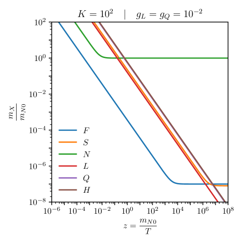
Figure 4: Evolution of the thermal masses. Due to a negligible difference between the thermal masses of $Q$, $u$, and $d$, we only show $m_{Q}$. In this regime, the thermal masses are basically independent of the initial $m_{X}(T=0)$ value. This is in contrast to the thermal mass of the right-handed neutrino whose thermal correction leave the large $m_{N0}=10^{10}~{}\mathrm{GeV}$ unchanged until small values of $z<10^{-2}$.

In order to study the impact of the additional contributions of our model, we choose $\epsilon=10^{-6}$ and $m_{N0}=10^{10}~{}\mathrm{GeV}$. We show the Boltzmann evolution for the yield of the right-handed neutrino $Y_{N}$ (blue solid line) and the yield of the ($B-L$) asymmetry in Fig. 5. We compare the $Y_{B-L}$ evolution of the standard scenario without (green dashed line) and with our new contributions (orange solid line). The evolution in the weak washout (left panels) and strong washout (right panels) regime is shown for two different example values $g_{L}=g_{Q}=\{10^{-2},10^{-3}\}$. Generally, we observe that the equilibrium yield of the right-handed neutrino $Y_{N}^{\mathrm{(eq)}}$ is reached much faster in the strong washout regime due to the larger decay rate (cp. Fig. 6, green solid line). Additionally, we present the evolution of the different, relevant contributions in Fig. 6.

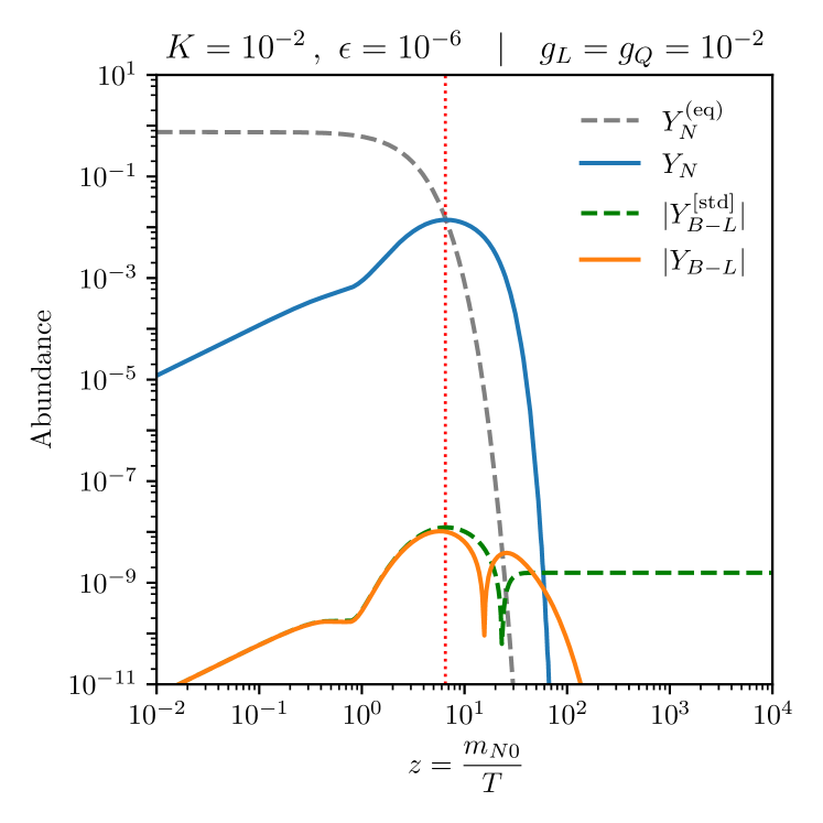
(a)

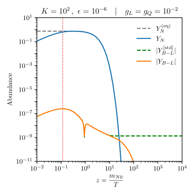
(b)

(c)

(d)

Figure 5: Evolution of the yield of the right-handed neutrino $Y_{N}$ (blue solid line) and the yield of the ($B-L$) asymmetry for the standard scenario $Y^{[\mathrm{std}]}_{B-L}$ (green dashed line) and including our new contributions $Y_{B-L}$ (orange solid line) for the weak (left panels) and strong (right panels) washout regime and two different example values for $g_{L}=g_{Q}=\{10^{-2},10^{-3}\}$. The equilibrium yield $Y_{N}^{\mathrm{(eq)}}$ is given as gray dashed line. The red dotted line indicates $z_{\mathrm{eq}}$.

(a)

(b)

(c)

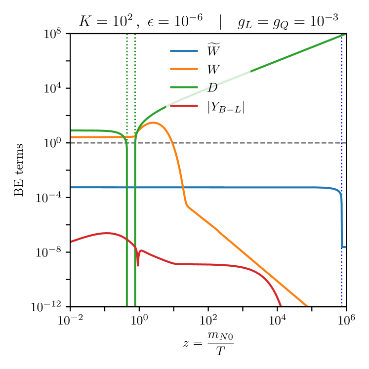
(d)

Figure 6: Evolution of the different contributions relevant for the yield of the ($B-L$) asymmetry $Y_{B-L}$ (orange solid line) for the weak (left panels) and strong (right panels) washout regime and two different example values for $g_{L}=g_{Q}=\{10^{-2},10^{-3}\}$. The green dotted lines show when $m_{H}(z)=m_{N}(z)+m_{L}(z)$ and $m_{N}(z)=m_{H}(z)+m_{L}(z)$, respectively. The blue dotted line shows when $m_{S}(z)=m_{F}(z)+m_{L}(z)$.

Scenario I ($\bm{g_{L}=g_{Q}=10^{-2}}$). As naively expected, for larger couplings, the largest effect of the new TeV-scale LNV washout terms can be observed. Comparing Figs. 5(a) and 6(a) (weak washout), we see that the constant behaviour of $Y_{B-L}$ at around $z\approx 0.6$ is caused by the dip that the decay rate $D$ receives due to the closing of $N\rightarrow HL$ and the opening of $H\rightarrow NL$ for small $z$. Even though the washout originating from $\widetilde{W}$ is stronger than the standard contribution $W$, it has no visible impact on the evolution of $Y_{B-L}$ (this picture changes for couplings of $\mathcal{O}(10^{-1})$). Around $z>7$, when the $W$ contribution decreases strongly, the $\widetilde{W}$ contribution remains constant and leads to a strong washout such that $Y_{B-L}$ falls below the observed value for the baryon asymmetry in contrast to the standard leptogenesis scenario.

A comparable situation is found for the strong washout regime (Figs. 5(b) and 6(b)). Due to the larger coupling, $y_{N}$, the washout originating from the standard leptogenesis scenario $W$ is now dominant $z<10$, see Fig. 6(b). Hence, the behavior of the standard leptogenesis scenario is followed longer up to larger $z$. However, when $W$ decreases significantly while $\widetilde{W}$ remains constant, $Y_{B-L}$ gets again fully washout out.

The $T$-independent washout term $\widetilde{W}$ in Fig. 6 can be understood as follows. The dominant contribution to $\widetilde{W}$ is given by the inverse decay $\widetilde{D}$ involving $F\leftrightarrow SL$ or $S\leftrightarrow FL$. This expression is a function of the decaying particle’s mass over temperature ($m_{F,S}/T$) and the right-handed neutrino mass ($m_{N}$). As shown in Fig. 4, for the relevant temperature range, both $m_{F}(T)$ and $m_{S}(T)$ are linear in temperature and $m_{N}(T)\approx m_{N0}$. Consequently, all quantities involved are effectively independent of the temperature.

The magnitude of $\widetilde{W}$ can be naively estimated from a power counting on the lepton number violating couplings, generically referred as $g$. Since this washout term is dominated by the inverse decay, and this process involves one lepton number violating vertex, then $\widetilde{W}=\mathcal{O}(g^{2})$. It is important to highlight the fact that, in a zero temperature approximation, the most relevant contribution to $\widetilde{W}^{T=0}$ is given by the scattering terms. Since these terms involve two lepton number violating vertices, it follows that $\widetilde{W}^{T=0}=\mathcal{O}(g^{4})$. Therefore, the inclusion of thermal effects is necessary to avoid an artificial suppression of the washout contribution coming from our simplified model. For lower temperatures, around $z=10^{6}$, the $\widetilde{D}$ contribution drops due to the mass hierarchy inversion, $m_{F}(T)\approx m_{S}(T)$, leading to the corresponding drop in $\widetilde{W}$.

Scenario II ($\bm{g_{L}=g_{Q}=10^{-3}}$). For smaller couplings, the washout contribution $\widetilde{W}$ is much smaller (see Figs. 6(c) and 6(d)) and only at later times dominant in comparison to the conventional washout processes. Hence, the $(B-L)$ asymmetry $Y_{B-L}$ drops below the observed baryon asymmetry also at later times for both the strong and weak washout scenario (see Figs. 5(c) and 5(d)).

Finally, we can relate the final yield $Y_{B-L}$ with the yield of the baryon asymmetry $Y_{B}$ Chen:2007fv ,

$$Y_{B}=\frac{28}{79}Y_{B-L}\,,$$ (41)

and compare it with the experimentally observed value in Eq. (2). The results are summarized in Fig. 7, choosing $m_{N0}=10^{10}~{}\mathrm{GeV}$. We show in red the parameter space that cannot account for the observed baryon asymmetry for the strong and weak washout scenario for two choices of the CP-asymmetry parameter, the usual choice $\epsilon=10^{-6}$ and the maximal possible CP-asymmetry $\epsilon=1$. As expected, the parameter space that implies a full wipe out of the baryon asymmetry created by the standard thermal leptogenesis does not depend on the lepton-number conserving coupling $g_{Q}$, but only on $g_{L}$. We observe that standard thermal leptogenesis is rendered unviable for lepton-number violating couplings $g_{L}$ of the order of $3\times 10^{-6}$ for $\epsilon=10^{-6}$ and $7\times 10^{-6}$ for $\epsilon=1$, respectively. Note that this is a conservative limit, as we have neglected the washout from scattering processes for numerical reasons as discussed before. Therefore, a discovery of lepton-number violating new physics at collider or ${0\nu\beta\beta}$-decay experiments in this parameter range would have far-reaching consequences on the validity of standard thermal leptogenesis.

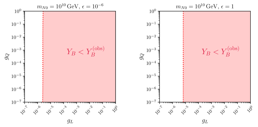
Figure 7: $g_{L}$-$g_{Q}$–plane for $\epsilon=10^{-6}$ (left panel) and $\epsilon=1$ (right panel), with $m_{N0}=10^{10}~{}\mathrm{GeV}$. The red area indicates the couplings that lead to a too strong washout and does not result in the observed baryon asymmetry. Considering the weak ($K=10^{-2}$) or strong ($K=10^{2}$) washout regime does not affect the plot visibly.

4 Collider study

The current experimental literature presents different results of various searches for LNV signals, ranging from specific decay modes of new particles (e.g., searches for $H^{\pm\pm}\to\ell^{\pm}\ell^{\pm}$ Chatrchyan:2012ya ; Aaboud:2017qph ) to comprehensive studies of BSM theories (e.g., Left-Right symmetric models Aaboud:2018spl or $R-$parity violating SUSY Chatrchyan:2013xsw ), including the connection with CP-violating effects at the LHC (e.g., rare $W$ decays Najafi:2020dkp ). The current status of those searches shows no evidence for significant deviations from the SM Khachatryan:2016kod ; Sirunyan:2017uyt .

The goal of our work is to study the interplay and complementarity between collider phenomenology and ${0\nu\beta\beta}-$decay experiments. Since the latter one involves both electrons and quarks –at a fundamental level–, our analysis is focused on studying the production of two same-sign electrons and two jets in a proton-proton collider, namely $pp\to jje^{\pm}e^{\pm}$. Our simplified model allows two topologies associated with the signal, as shown in Fig. 8.

Figure 8: Feynman diagrams of the two-jet, same-sign dilepton signal ($pp\to e^{\pm}e^{\pm}jj$) in our simplified model. Diagram (a) matches the ${0\nu\beta\beta}-$decay diagram in Fig. 2.

In principle, some direct searches might also restrict our model. The first term in Eq. 5 makes this model sensitive to current experimental limits from di-jet resonant production. The ATLAS collaboration has recently published searches for low-mass Aaboud:2019zxd and high-mass Aad:2019hjw resonances in mass distributions of two jets. Reinterpreting those results, specifically the generic Gaussian-shaped distributions, we find that values for $g_{Q}\gtrsim 0.1$ are roughly excluded for our parameter region of interest. The second term in Eq. 5 shows a potential sensitivity to single lepton plus missing $E_{T}$ searches CMS:2021pmn if $F$ decays outside the detector. However, based on our estimations for the decay length Banerjee:2019ktv , we conclude that $F$ will decay promptly for the parameter region of interest.

4.1 Event generation and classification

To perform our collider study, we have implemented the model (5) using FeynRules Alloul:2013bka to generate events with Madgraph Alwall:2014hca at the parton level. We rely on PYTHIA Sjostrand:2014zea for parton showering and jet matching, and Delphes deFavereau:2013fsa for fast detector simulation. For both, signal and background, we impose a set of basic selection cuts ($p_{T_{j}},p_{T_{\ell}}>20\,\mathrm{GeV}$, $|\eta_{j}|<2.8$, $|\eta_{\ell}|<2.5$) at the generator level Peng:2015haa , and a pre-selection rule ($N_{j}\geq 2$, $N_{\ell^{\pm}\ell^{\pm}}\geq 2$) at the classification level.

Our analysis is focused on the potential reach of the LHC at 14 TeV, in addition to the hypothetical FCC-hh Mangano:2017tke and SppC Tang:2015qga at 100 TeV. The Delphes software package deFavereau:2013fsa incorporates the configuration card for ATLAS and CMS detectors at the LHC, while the equivalent one for the FCC-hh baseline detector is available online and a detailed description of the implementation is available in Ref. Selvaggi:2717698 .

The event classification is based on a custom-made Recurrent Neural Network (RNN) inspired by previous experiences Paganini:2157570 in the context of event discrimination using Deep Learning. An RNN allows us to classify events with unordered, variable length inputs, such as the number of jets or electrons Guest:2016iqz . Our implementation uses the kinematic properties of jets, electrons, and missing $E_{T}$ to differentiate signal-like and background-like events. A detailed description of our topology is given in Appendix A.2 where we have also included a brief introduction to RNNs.

Additionally, we also implemented a Boosted Decision Tree (BDT) to compare these two machine learning approaches’ results. We found that both the RNN and the BDT implementations presented a similar performance, consistent with previous comparisons available in the literature Bradshaw:2019ipy ; Alves:2016htj ; Buzatu:2651122 . As both implementations have similar performance, our choice of using an RNN is based on its ease of use since it offers a little more flexibility than a BDT.

4.2 Signal generation and phenomenology

The cross section associated with a $t-$channel production in Fig. 8, $\sigma_{[t]}$, has a coupling dependence given by $(g_{L}\,g_{Q})^{4}$ and it is relatively insensitive of the mass hierarchy between $F$ and $S^{\pm}$. Additionally, the $s-$channel cross section in Fig. 8, $\sigma_{[s]}$, always involves the production of an on-shell particle. These two facts make the latest one to dominate the cross section over the first one, $\sigma(pp\to jje^{\pm}e^{\pm})\approx\sigma_{[s]}(pp\to jje^{\pm}e^{\pm})$. Consequently, the behavior of diagram (b) gives us insights about the total cross section.

To understand the coupling dependence of $\sigma_{[s]}$, notice that the physical processes vary depending on the mass hierarchy due to kinematic constraints as summarized in Table 1. Each sub-process corresponds to the successive production or decay chains of the signal.

Case	Mass hierarchy	Process
C1	$m_{S}<m_{F}$	$pp\to e^{\pm}F$,	$F\to e^{\pm}S^{\mp}$,	$S^{\mp}\to jj$
C2	$m_{S}=m_{F}$	$pp\to e^{\pm}F$,	$F\to e^{\pm}jj$
C3	$m_{S}>m_{F}$	$pp\to S^{\pm}$,	$S^{\pm}\to e^{\pm}F$,	$F\to e^{\pm}jj$

Table 1: Kinematic classification of production and successive decays involved in diagram (b), Fig. 8, in our simplified model.

If we use the narrow-width approximation, it is possible to decompose the different sub-processes in Table 1 in the following manner:

• When $F$ is heavier than $S^{\pm}$, the cross section corresponds to the production of an on-shell $F$ in addition to an electron –with $\sigma_{[s]}(pp\to e^{\pm}F)\propto(g_{L}\,g_{Q})^{2}$– followed by two cascade decays. These decay modes have branching ratios that are coupling independent since those are the only ones kinematically allowed:

  $$\sigma_{[s]}(pp\to e^{\pm}e^{\pm}jj)=\underbrace{\sigma_{[s]}(pp\to e^{\pm}F)}_{\propto\ (g_{L}\,g_{Q})^{2}}\times\underbrace{\mathrm{Br}(F\to e^{\pm}S^{\mp})}_{=\ 2/3}\times\underbrace{\mathrm{Br}(S^{\pm}\to jj)}_{=\ 1}\,.$$ (42)

• In the same fashion, if both $S^{\pm}$ and $F$ have equal masses then the cross section also corresponds to the production of an on-shell $F$ accompanied by an electron, followed by the decay of $F$ into a pair of jets and an electron. This decay, again, is the only one possible –so it has a branching ratio equal to one– and it is mediated by an off-shell $S^{\pm}$ propagator:

  $$\sigma_{[s]}(pp\to e^{\pm}e^{\pm}jj)=\underbrace{\sigma_{[s]}(pp\to e^{\pm}F)}_{\propto\ (g_{L}\,g_{Q})^{2}}\times\underbrace{\mathrm{Br}(F\to e^{\pm}jj)}_{=\ 2/3}\,.$$ (43)

• Finally, the case where $m_{S}>m_{F}$ provides a more subtle dependence. The full cross section can be thought as the on-shell production of $S^{\pm}$ –with $\sigma_{[s]}(pp\to S^{\pm})\propto g_{Q}{}^{2}$– followed by two successive decays. In this regime, $S^{\pm}$ is allowed to decay into two jets or a pair $e^{\pm}F$. The branching ratio is a function of the two couplings, as shown in Eq. 44:

  $$\sigma_{[s]}(pp\to e^{\pm}e^{\pm}jj)=\underbrace{\sigma_{[s]}(pp\to S^{\pm})}_{\propto\ g_{Q}{}^{2}}\times\underbrace{\mathrm{Br}(S^{\pm}\to e^{\pm}F)}_{=\ \left[1+\kappa\,\left(\frac{g_{Q}}{g_{L}}\right)^{2}\right]^{-1}}\times\underbrace{\mathrm{Br}(F\to e^{\pm}jj)}_{=\ 2/3}\,,$$ (44)

  where $\kappa$ depends on the ratio between the two masses satisfying $\kappa>1$ for $m_{S}>m_{F}$. It is worthwhile to highlight two limiting cases:

  • If $g_{Q}\gg g_{L}$, then $\mathrm{Br}(S^{\pm}\to e^{\pm}F)\propto(g_{L}/g_{Q})^{2}$ and the cross section scales with $g_{L}{}^{2}$.

  • If $g_{Q}\ll g_{L}$, then the $\mathrm{Br}(S^{\pm}\to e^{\pm}F)\approx 1$ and the cross section scales with $g_{Q}{}^{2}$.
    

A key difference between the three cases is the magnitude of the respective cross sections. To illustrate, consider the production cross sections in cases C1-C2 and C3, i.e., $\sigma_{[s]}(pp\to e^{\pm}F)$ and $\sigma_{[s]}(pp\to S^{\pm})$, respectively. In the first one, notice that the momentum transfer along the $s-$channel needed to produce an on-shell $F$ implies a suppression since the particle in the propagator is off-shell. However, the production in the latest one directly creates an on-shell $S^{\pm}$ so no suppression is applied. The different order in the couplings reinforces the difference between the magnitudes of the cross sections for the same set of parameters, as we illustrate in Table 2.

	$m_{S}=0.5\,\mathrm{TeV}$	$m_{S}=2\,\mathrm{TeV}$
$\sigma(pp\to jje^{\pm}e^{\pm})$	$1.199\times 10^{-8}\,\mathrm{pb}$	$8.874\times 10^{-5}\,\mathrm{pb}$
$\sigma_{[s]}(pp\to jje^{\pm}e^{\pm})$	$1.195\times 10^{-8}\,\mathrm{pb}$	$8.874\times 10^{-5}\,\mathrm{pb}$
Production mode	$pp\to e^{\pm}F$	$pp\to S^{\pm}$
Production cross section	$4.012\times 10^{-8}\,\mathrm{pb}$	$3.545\times 10^{-4}\,\mathrm{pb}$

Table 2: Numerical example of the phenomenological behavior of the signal cross section at $\sqrt{s}=14\,\mathrm{TeV}$. We took $m_{F}=1\,\mathrm{TeV}$, $g_{L}=0.1$, and $g_{Q}=0.01$ in both scenarios. The results were obtained from Madgraph Alwall:2014hca .

4.3 Background generation and validation

Backgrounds in the same-sign dilepton final state can be divided into three categories Khachatryan:2016kod :

• SM processes with same-sign dileptons, including diboson production (considering $W$, $Z$, $H$, and prompt $\gamma$), single boson production in association with a $t\overline{t}$ pair, and “rare” processes (e.g., $t\overline{t}t\overline{t}$ and double-parton scattering).

• Charge misidentification from events with opposite-sign isolated leptons in which the charge of an electron is misidentified, mostly due to severe bremsstrahlung in the tracker material.

• Jet-fake leptons from heavy-flavor decays, where hadrons are misidentified as leptons, or electrons from unidentified conversions of photons in jets.

For our analysis, we study the effects of the dominant contributions: EW diboson processes, charge misidentification involving $\gamma/Z^{\ast}$, and jet-fakes produced by $t\overline{t}$ and $W+3j$ processes Peng:2015haa ; Sirunyan:2017uyt . The diboson simulation involved the generation of $WW$, $WZ$, and $ZZ$ events plus jets, and their respective leptonic decays, as implemented in Ref. Peng:2015haa .

Due to the difficulty of precisely simulating jet-fakes, we implement the “FakeSim” method proposed in Ref. Curtin:2013zua as an additional module in Delphes. This data-driven approach takes into account the relation between the originating jet and the fake lepton. It is based on two functions:

1. A mistag efficiency, $\epsilon_{j\to\ell}(p_{T_{j}})$, representing the probability that a particular jet $j$ is mistagged as a lepton $\ell$.

2. A transfer function, $\mathcal{T}_{j\to\ell}$, modeling the probability distribution function that maps $p_{T_{j}}$ into the fake $p_{T_{\ell}}$.

Using data or simulations from ATLAS or CMS collaborations, it is possible to fit the set of parameters to find consistent results for different phenomenological studies Izaguirre:2015pga ; Dib:2016wge ; Nemevsek:2016enw . In Fig. 9, we compare representative CMS results (digitized from Fig. 3 in Ref. Sirunyan:2017uyt ) with our result obtained using the FakeSim method. As can be seen from the plot, we reproduce the overall behavior after a parameter fitting. It is possible to optimize the choice of the FakeSim parameters if, for instance, flavor effects are included by introducing flavor-dependent mistag efficiencies Priv_Comm_Li .

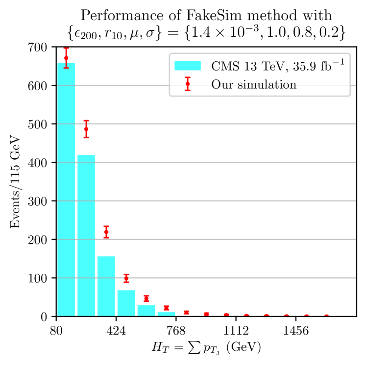
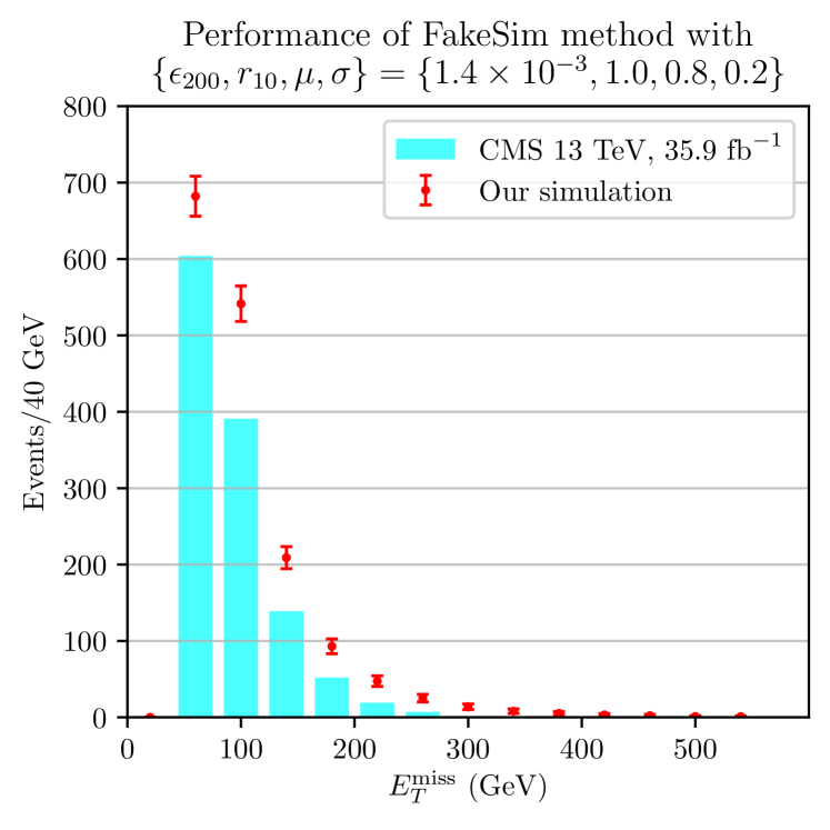
Figure 9: Comparison between the CMS results in Ref. Sirunyan:2017uyt and our implementation of the FakeSim method proposed in Ref. Curtin:2013zua for a particular choice of its parameters, as mentioned in Note (3). Distributions of the kinematic variables $H_{T}$ and $E_{T}^{\mathrm{miss}}$ are shown in the left and right panels, respectively.

To estimate the charge misidentification background, we introduce a misidentification probability for electrons from current doubly charged Higgs boson searches by the ATLAS collaboration Aaboud:2017qph . The electron charge misidentification probability is modeled as a separable function of electron’s $p_{T}$ and $\eta$, $P(p_{T},\eta)=\sigma(p_{T})f(\eta)$, and its data-driven values are extracted from Fig. 3 in Ref. Aaboud:2017qph . We follow a common approach in collider phenomenological studies Helo:2018rll ; Pan:2019wwv to incorporate this probability as a weight in opposite-sign generated events, as detailed in Section 7.1.3 in Ref. Muskinja:2643902 . In Table 3, we compare our background estimation with the ATLAS results extracted from Fig. 2 in Ref. Aaboud:2017qph for a $Z\to ee$ peak data sample. The ratio of same-charge/opposite-charge events for ATLAS is 0.93% and we obtained 0.70%.

	Number of events
	Opposite-charge	Same-charge	SC/OC
	(OC)	(SC)	ratio
ATLAS	$1.23\times 10^{7}$	$1.14\times 10^{5}$	0.93%
Our estimation	$9.41\times 10^{6}$	$6.59\times 10^{4}$	0.70%

Table 3: Validation of the charge misidentification implementation. The ATLAS results extracted from Fig. 2 in Ref. Aaboud:2017qph , and our results make use of the probability density defined in Ref. Muskinja:2643902 .

Notice that the two data-driven methods previously described were validated using LHC data. Table 4 presents the background cross section for the three classes, detailing the effects of the signal selection rule $(N_{j}\geq 2,\ N_{\ell^{\pm}\ell^{\pm}}\geq 2)$ and the background discrimination by using the RNN. The first column shows the cross section before the signal selection ($\sigma_{\mathrm{before}}$), as given directly by Madgraph. The second column shows the cross sector after applying the signal selection rule ($\sigma_{\mathrm{after}}$), where the number of events is initially reduced. Finally, the third column shows the background cross section classified by the RNN ($\sigma_{\mathrm{RNN}}$), and we notice the background reduction provided by our machine learning implementation. Since there are no estimations for these types of background for a future 100 TeV hadron collider, we use the same set of parameters and functions varying only the energy of the center of mass. Table 5 presents the results of our estimation.

Background type		$\sigma_{\mathrm{before}}$ (pb)	$\sigma_{\mathrm{after}}$ (pb)	$\sigma_{\mathrm{RNN}}$ (pb)
Diboson	$WW$	$3.28\times 10^{-3}$	$6.40\times 10^{-4}$	$6.87\times 10^{-5}$
	$WZ$	$2.59\times 10^{-2}$	$6.65\times 10^{-3}$	$2.10\times 10^{-4}$
	$ZZ$	$1.32\times 10^{-3}$	$5.62\times 10^{-4}$	$1.14\times 10^{-5}$
Jet-fake	$W+3j$	$1.79\times 10^{-1}$	$4.34\times 10^{-2}$	$1.78\times 10^{-4}$
	$t\bar{t}$	$9.11\times 10^{-2}$	$2.64\times 10^{-2}$	$6.10\times 10^{-5}$
Charge misidentification	$t\bar{t}$	$3.33\times 10^{-2}$	$1.54\times 10^{-2}$	$4.45\times 10^{-4}$
	$Z/\gamma^{\ast}$	$2.54\times 10^{-1}$	$1.37\times 10^{-1}$	$4.89\times 10^{-3}$
		$5.88\times 10^{-1}$	$2.30\times 10^{-1}$	$5.86\times 10^{-3}$

Table 4: Individual contributions to the cross section for the different types of background for the LHC at 14 TeV. $\sigma_{\mathrm{before}}$ corresponds to the cross section before the signal selection, $\sigma_{\mathrm{after}}$ corresponds to the cross section after the signal selection, and $\sigma_{\mathrm{RNN}}$ is the cross section tagged as background events by the RNN. The last row shows the total background cross section.

Background type		$\sigma_{\mathrm{before}}$ (pb)	$\sigma_{\mathrm{after}}$ (pb)	$\sigma_{\mathrm{RNN}}$ (pb)
Diboson	$WW$	$3.56\times 10^{-2}$	$1.76\times 10^{-2}$	$2.27\times 10^{-3}$
	$WZ$	$3.78\times 10^{-1}$	$1.88\times 10^{-1}$	$5.88\times 10^{-3}$
	$ZZ$	$1.95\times 10^{-2}$	$1.35\times 10^{-2}$	$2.53\times 10^{-4}$
Jet-fake	$W+3j$	$2.21$	$7.16\times 10^{-1}$	$6.72\times 10^{-3}$
	$t\bar{t}$	$3.85$	$1.43$	$6.82\times 10^{-3}$
Charge misidentification	$t\bar{t}$	$5.11\times 10^{-1}$	$3.36$	$1.60\times 10^{-1}$
	$Z/\gamma^{\ast}$	$3.33$	$2.02$	$1.51\times 10^{-1}$
		$10.33$	$7.75$	$3.33\times 10^{-1}$

Table 5: Individual contributions to the cross section for the different types of background for the FCC-hh at 100 TeV. The definitions of $\sigma_{\mathrm{before}}$, $\sigma_{\mathrm{after}}$, and $\sigma_{\mathrm{RNN}}$ are equivalent as in Table 4. The last row shows the total background cross section.

5 ${0\nu\beta\beta}$ Decay

The results from searches for ${0\nu\beta\beta}$ place complementary constraints on the model parameters in a manner that can complement the collider search results. However, in order to account for the different scales, we need to evolve the operator $\mathcal{O}_{1}$ in Eq. (7) from the TeV scale to the GeV scale using renormalization group running. Hereby, operators receive QCD and electroweak corrections and mix with other operators. The RGE evolution was studied in Ref. Peng:2015haa , with the dominant QCD corrections considered. The relevant part of $\mathcal{O}_{1}$ contributing to ${0\nu\beta\beta}$-decay is:

$$\mathscr{L}_{\mathit{LNV}}^{\mathrm{eff}}=\frac{C_{\mathrm{eff}}}{2\Lambda^{5}}\left(\mathcal{O}_{2+}^{++}-\mathcal{O}_{2-}^{++}\right)\overline{e_{L}}e_{R}^{c}\ +\ \mathrm{h.c.}\,,$$ (45)

where $e_{R}^{c}\equiv(e_{L})^{c}$, $C_{\mathrm{eff}}\approx C_{1}(1\,\mathrm{GeV})=0.092C_{1}(\Lambda)$ Peng:2015haa , and the operator $\mathcal{O}_{2}$ being Prezeau:2003xn :

$$\mathcal{O}_{2\pm}^{ab}=(\bar{q}_{R}\tau^{a}Q)(\bar{q}_{R}\tau^{b}Q)\pm(\bar{Q}\tau^{a}q_{R})(\bar{Q}\tau^{b}q_{R})\,.$$ (46)

When $a=b$, the operator with subscript $+(-)$ are even (odd) eigenstates of parity. As the hadronic (four quark) part of the operator carries no dependence on the lepton kinematics, the matrix element for the process factorizes into a leptonic and hadronic part. Computation of the former is straightforward. For the latter, we first match the four-quark operator $\mathcal{O}_{2+}^{++}-\mathcal{O}_{2-}^{++}$ onto hadronic degrees of freedom most appropriate for computation of the nuclear transition matrix element, following the effective field theory (EFT) approach delineated in Refs. Prezeau:2003xn ; Cirigliano:2018yza . The leading order contribution to the nuclear matrix element (NME) arises from the pion-exchange amplitude of Fig. 10, where the LNV $\pi\pi ee$ interaction emerges from matching $\mathcal{O}_{2+}^{++}{\bar{e}_{L}}e_{R}^{c}$ onto the two pion-two electron operator in Eq. 45:

$$\frac{C_{\mathrm{eff}}\Lambda_{H}^{2}F_{\pi}^{2}}{2\Lambda^{5}}\pi^{-}\pi^{-}{\bar{e}_{L}}e_{R}^{c}+\mathrm{h.c.}\,,$$ (47)

where $F_{\pi}=92.2\pm 0.2$ MeV is the pion decay constant DGH:14 and $\Lambda_{H}$ is a mass scale associated with the hadronic matrix element (HME) of the four quark operator $\mathcal{O}_{2+}^{++}$,

$$\Lambda_{H}^{2}F_{\pi}^{2}=\frac{1}{2}\left\langle 0\right\rvert\left(\mathcal{O}_{2+}^{++}-\mathcal{O}_{2-}^{++}\right)\left\lvert\pi^{-}\pi^{-}\right\rangle\,.$$ (48)

In the earlier work of Ref. Peng:2015haa $\Lambda_{H}^{2}$ was obtained using factorization/vacuum saturation to estimate the HME, yielding $\Lambda_{H}^{2}=m_{\pi}^{4}/(m_{u}+m_{d})^{2}\approx-7.5$ GeV² for $m_{\pi^{+}}=139$ MeV and $m_{u}+m_{d}=7$ MeV. Subsequently, the authors of Ref. Cirigliano:2017ymo noted that one may relate $\mathcal{O}_{2+}^{++}$ to analogous $\Delta S\not=0$ four-quark operators using SU(3) flavor symmetry. Consequently, one may exploit flavor SU(3) to obtain estimates of $\Lambda_{H}^{2}$ from the corresponding strangeness changing $K^{0}\to{\bar{K}^{0}}$ and $K\to\pi\pi$ matrix elements. The result yields $\Lambda_{H}^{2}=-(3.16\pm 0.7)$ GeV² at the matching scale $\mu=3$ GeV. The Cal-Lat collaboration performed a direct computation of the matrix element in Eq. (48), obtaining $\Lambda_{H}^{2}=-(2.15\pm 0.36)$ GeV² at $\mu=3$ GeV in the RI/SMOM scheme Nicholson:2018mwc . In what follows, we will adopt the Cal-Lat value.

When used to evaluate the amplitude in Fig. 10, the interaction in Eq. (47) yields an effectivce two nucleon-two electron operator whose nuclear matrix elements (NMEs) may be evaluated using state-of-the-art many-body methods. The resulting expression for the decay rate is

$$\frac{1}{T_{1/2}} = \left[G_{0\nu}\times(1\,\mathrm{TeV})^{2}\right]\left(\frac{\Lambda_{H}}{\mathrm{TeV}}\right)^{4}\left(\frac{1}{144}\right)$$

$$\times \left(\frac{v}{\mathrm{TeV}}\right)^{8}\left(\frac{1}{\cos\theta_{C}}\right)^{4}|M_{0}|^{2}\,\left[\frac{C_{\mathrm{eff}}^{2}}{(\Lambda/\mathrm{TeV})^{10}}\right]\ \ \ ,$$

$$G_{0\nu} = (G_{F}\cos\theta_{C}g_{A})^{4}\left(\frac{\hbar c}{R}\right)^{2}\left(\frac{1}{32\pi^{2}\hbar\ln 2}\right)I(E_{\beta\beta})\ \ \ ,$$

with $\theta_{C}$ being the Cbibbo angle, $I(E_{\beta\beta})$ the electron phase space integral

$$\int_{m_{e}}^{E_{\beta\beta}-m_{e}}dE_{1}\,F(Z+2,E_{1})F(Z+2,E_{2})p_{1}E_{1}p_{2}E_{2}\ \ \ ,$$ (50)

$E_{2}=E_{\beta\beta}-E_{1}$, and $F(Z+2,E_{1,2})$ being factors that account for distortion of the electron wave functions in the field of the final state nucleus. The NME is given by

$$M_{0}=\left\langle{\Psi_{f}}\right|\sum_{i\not=j}\frac{R}{\rho_{ij}}\left[F_{1}{\vec{\sigma}}_{i}\cdot{\vec{\sigma}}_{j}+F_{2}T_{ij}\right]\tau^{+}_{i}\tau^{+}_{j}\left|{\Psi_{i}}\right\rangle\,,$$ (51)

where $T_{ij}=3{\vec{\sigma}}_{i}\cdot{\hat{\rho}}_{ij}{\vec{\sigma}}_{j}\cdot{\hat{\rho}}_{ij}-{\vec{\sigma}}_{i}\cdot{\vec{\sigma}}_{j}$, $R=r_{0}A^{1/3}$, ${\vec{\rho}}_{ij}$ is the separation between nucleons $i$ and $j$, and the functions $F_{1,2}(|\vec{\rho}_{ij}|)$ are given in Ref. Prezeau:2003xn . Note that we have normalized the rate to the conventionally-used factor $G_{0\nu}$ that contains quantities associated with the SM weak interaction, even though the LNV mechanism here involves no SM gauge bosons. Note also that Eq. (5) corrects two errors in the corresponding expression in Ref. Peng:2015haa : (a) the inclusion here of a factor of $g_{A}^{4}$ and (b) an additional overall factor of $1/8$. The latter arises from a factor of $1/2$ due to the presence of two electrons in the final state and a factor of $(1/2)^{2}$ that one must include to avoid double counting in the NME since the sum runs over $i\not=j$ rather than $i<j$.

In the analysis of Ref. Peng:2015haa , a value of $M_{0}=-1.99$ for the transition ${{}^{76}\mathrm{Ge}}\to{{}^{76}\mathrm{Se}}$ was adopted from the quasiparticle random phase approximation (QRPA) computation of Ref. Faessler:1998qv . Here, we use the results of a more recent proton-neutron (pn) QRPA computation of Ref. Hyvarinen:2015bda . The resulting value for $M_{0}({{}^{76}\mathrm{Ge}}\to{{}^{76}\mathrm{Se}})=-4.74$. At present, the most sensitive limit on the half life has been obtained using ¹³⁶Xe, for which the matrix element in Ref. Hyvarinen:2015bda is $M_{0}({{}^{136}\mathrm{Xe}}\to{{}^{136}\mathrm{Ba}})=-2.63$. Both pnQRPA values assume no “quenching” of $g_{A}$.

It is important to emphasize that the calculated NMEs exhibit considerable theoretical uncertainties. The earlier work of Ref. Peng:2015haa accounted for the combined effect of these uncertainties as well as those in HMEs by varying the value of $M_{0}$ by a factor of two. The subsequent chiral SU(3) and lattice computations of $\left\langle 0\right\rvert\mathcal{O}_{2+}^{++}\left\lvert\pi^{-}\pi^{-}\right\rangle$ have reduced the hadronic uncertainty to the $\mathcal{O}(10\%)$ level. In the case of the NME, however, it has been realized that in the context of few-nucleon effective field theory, consistent renormalization requires the presence of a contact interaction in addition to the long-range two-pion exchange amplitude Cirigliano:2018hja . The corresponding operator coefficient and nuclear matrix element are presently unknown. We thus retain a factor of two uncertainty in the NME to account for both the bona fide nuclear many-body uncertainties as well as the effect of the “counterterm” contribution.

Figure 10: Contribution of dim-9 LNV $\pi\pi ee$ interaction to ${0\nu\beta\beta}-$decay at tree level.

6 Combined results and discussion

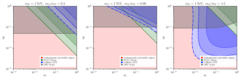
Figure 11: Interplay between leptogenesis, collider searches, and ${0\nu\beta\beta}-$decay experiments for $m_{F}=1$ TeV, and $m_{S}/m_{F}=\{0.5,0.99,1.5\}$. As in Fig. 7, we present the nonviable leptogenesis region in red; in dark green, we show the ${0\nu\beta\beta}-$decay exclusion from KamLAND-Zen (dotted line) and future tonne-scale experiments (dashed line); the collider LNV (same sign dilepton plus dijet) exclusion is shown in blue for the LHC at 14 TeV with integrated luminosities of 100 fb^-1 (dotted line) and 3 ab^-1 (dashed line), and the FCC-hh at 100 TeV with 30 ab^-1 (dash-dotted line); and, in dark gray, we present the LHC di-jet exclusion, as discussed in Section 4.

In the following, we combine our results from the previous sections in order to investigate the reach and interplay of collider and ${0\nu\beta\beta}$-decay experiments and the implications of a possible discovery for the generation of the baryon asymmetry.

In Fig. 7, we illustrated the parameter space (red) that was found to lead to a baryon asymmetry smaller than the observed one because of to a too strong washout due to the new TeV-scale interactions. Fixing the masses of the new particles $F$ and $S$ around the TeV scale, we can read off the couplings $g_{L}$ and $g_{Q}$ for which we would expect a strong washout that would prevent a large enough baryon asymmetry. Hence, a discovery of a process within this parameter space would preclude the viability of the standard thermal leptogenesis scenario.

As depicted in Fig. 2, the new interactions in the Lagrangian, Eq. (5), can lead to ${0\nu\beta\beta}$-decay. We show in green in Fig. 11, the region currently excluded region by KamLAND-Zen (green dotted line), but also the future reach of tonne-scale experiments (green dashed line). With this region lying in the red area, we can conclude that an observation of ${0\nu\beta\beta}$-decay realized by a dim-9 operator with new physics at the TeV scale would rule out the standard leptogenesis paradigm. As demonstrated in Fig. 7 (right), this conclusion remains valid even for the most optimistic choice of maximal CP asymmetry.

With ${0\nu\beta\beta}$-decay being a low energy process, it is not sensitive to the mass hierarchy $m_{S}/m_{F}$ and explicit couplings $g_{L}$ and $g_{Q}$ of the new degrees of freedom at the TeV scale, but only to the effective coupling $C_{1}$ and scale $\Lambda$, as stated in Eq. (8). Therefore, the decreased reach from left to right in Fig. 11, is caused by the increase in $\Lambda$, leading to a suppression of the process.

High-energy collider experiments, however, can resolve the TeV-mass scale, and hence depend on the mass hierarchy of the new particles $F$ and $S$. We show the current 14 TeV collider limits with $100~{}\mathrm{fb}^{-1}$ integrated luminosity for the different mass hierachies (blue dotted line), as well as for future $3~{}\mathrm{ab}^{-1}$ integrated luminosity (blue dashed line) and the FCC-hh with 100 TeV and $30~{}\mathrm{ab}^{-1}$ (blue dashed-dotted line). As discussed in detail in Sec. 4, the mass hierarchy is crucial for the reach of the collider searches. For $m_{S}>m_{F}$, $S$ can be produced resonantly followed by subsequent decays into a signature of two same-sign electrons and two jets, leading to the strongest constraints (see the dominant s-channel process depicted in Fig. 8 (b)). We also reiterate that for $g_{Q}>g_{L}$ the limits are mainly restricted by $g^{2}_{L}$ and independent of $g_{Q}$, while for $g_{L}>g_{Q}$ the limits are mainly constrained by $g^{2}_{Q}$ (and not $g_{L}$). For $m_{S}\lesssim m_{F}$, in contrast, the collider constraints are much weaker, as $S$ can be produced only off-shell. If we compare the the current and future collider sensitivities (blue) to the red region for all three mass hierarchies, we see that an observation of two same-sign electrons and two jets would similarly rule out the standard thermal leptogenesis scenario for weak and strong washout.

While a same sign di-electron plus di-jet signature directly points to a LNV process, direct searches for the particles $F$ and $S$ also constrain the model parameter space. We show the limits from dijet resonant searches in gray. While covering already the full collider reach for $m_{S}\lesssim m_{F}$, they are less sensitive for $m_{S}>m_{F}$. The interplay of the di-jet, same sign di-electron, and $0\nu\beta\beta$-decay sensitivities in Fig. 11 illustrates the complementarity of these probes. Drawing on all of them will be important if a non-zero LNV signal is seen at either low- or high-energies.

As apparent from Fig. 11, the relative reaches of ${0\nu\beta\beta}$-decay experiments and collider LNV searches depend decisively on the new particle spectrum. This emphasizes the importance of pursuing and combining the low- and high-energy frontier in order to cover wide ranges of the parameter space but also to identify, in case of an observation, the underlying new physics. For instance, for $m_{S}\gtrsim m_{F}$, the observation of ${0\nu\beta\beta}$-decay would imply an observable signal at the LHC or would point towards another underlying $0\nu\beta\beta$-decay mechanism.

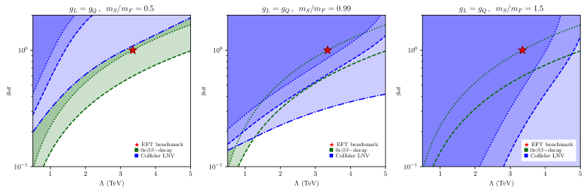
Figure 12: Complementarity between collider searches and ${0\nu\beta\beta}-$decay experiments for $g_{L}=g_{Q}$ and $m_{S}/m_{F}=\{0.5,0.99,1.5\}$. Comparison with an EFT analysis for the scale of new physics $\Lambda=(m_{S}^{4}m_{F})^{1/5}$ and the effective coupling $g_{\mathrm{eff}}=g_{L}=g_{Q}$. In dark green, we show the ${0\nu\beta\beta}-$decay exclusion from KamLAND-Zen (dotted line) and future tonne-scale experiments (dashed line); and the collider LNV exclusion is shown in blue for the LHC at 14 TeV with integrated luminosities of 100 fb^-1 (dotted line) and 3 ab^-1 (dashed line), and the FCC-hh at 100 TeV with 30 ab^-1 (dash-dotted line). The EFT benchmark point is shown as a red star, where $g_{\mathrm{eff}}=1$ is assumed for the discussion.

It is interesting to compare our simplified model results with those obtained using the EFT framework. To that end, we show in Fig. 12 the effective coupling $g_{\mathrm{eff}}=g_{L}=g_{Q}=C_{1}^{1/4}$ versus the scale of new physics $\Lambda=(m_{S}^{4}\,m_{F})^{1/5}$ for the different mass hierarchies shown in the previous figures. Note that we fix the absolute masses $m_{F},m_{S}$ only indirectly via the scale $\Lambda$. We indicate the limit on the scale of new physics when naively assuming $g_{\mathrm{eff}}=g_{L}=g_{Q}=1$ with a red star. Comparing the three different panels, it becomes again obvious that whether $0\nu\beta\beta$ decay or collider searches are more sensitive crucially depends on the relative mass hierarchy. As $0\nu\beta\beta$ decay is cannot resolve the heavy new physics, combining both experimental approaches is crucial.

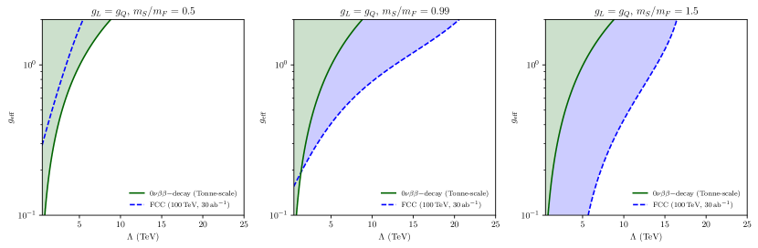
Figure 13: Complementarity between the next generation of colliders and ${0\nu\beta\beta}-$decay experiments for $g_{L}=g_{Q}$ and $m_{S}/m_{F}=\{0.5,0.99,1.5\}$. The definitions of $\Lambda$ and $g_{\mathrm{eff}}$ are the same as in Fig. 12. In dark green, we show the ${0\nu\beta\beta}-$decay exclusion from future tonne-scale experiments, and the reach the FCC-hh LNV searches at 100 TeV with 30 ab^-1 is shown in blue.

In Fig. 13, we finally show a similar set of plots, in which we allow for a larger new physics scale $\Lambda$, demonstrating the future reach of a tonne-scale $0\nu\beta\beta$-decay experiment and the FCC-hh. While $0\nu\beta\beta$-decay experiments will reach a sensitivity of $\Lambda\approx 10~{}\mathrm{TeV}$, the FCC-hh will reach between $\Lambda\approx 5~{}\mathrm{TeV}$ and $\Lambda\approx 15~{}\mathrm{TeV}$, depending on the mass hierarchy.

These results demonstrate that observing a LNV signal at $0\nu\beta\beta$-decay or collider experiments has the potential to exclude the standard thermal leptogenesis scenario. Given their complementary experimental reach, the combination of the high- and low-energy frontier is crucial to probe the mechanism behind the baryon asymmetry generation.

7 Conclusions

The observation of LNV would have profound implications for our understanding of nature, from the origin of neutrino masses to the matter-antimatter asymmetry of the Universe. In this work, we studied the interplay between three different physical aspects linked by LNV at the TeV scale: ${0\nu\beta\beta}$-decay, collider phenomenology, and thermal leptogenesis. Previous studies have been performed Deppisch:2015yqa ; Deppisch:2017ecm from an effective field theory (EFT) standpoint, showing the complementarity between current and future experimental results and their potential to falsify the standard thermal leptogenesis mechanism as explanation for the origin of matter. We extended previous work by focusing on a concrete, simplified model in order to study aspects that are not possible to capture by an EFT approach such as different mass hierarchies of the new physics involved.

To this end, we considered the SM extended by at least two right-handed neutrinos leading to neutrino masses via the Type I see-saw mechanism and additionally a scalar doublet $S$ and a Majorana singlet $F$, both having masses around the TeV-scale. This model was introduced in Ref. Peng:2015haa , where the interplay between collider searches at the LHC and ${0\nu\beta\beta}$-decay experiments was studied. Besides a detailed analysis of the implications of a possible observation of a $\Delta L=2$ lepton-number violating signal for the validity of standard thermal leptogenesis, we extended previous works by using the latest hadronic and nuclear matrix elements, improving on the derivation of the ${0\nu\beta\beta}$-decay half-life, and updating the corresponding predictions.

We also revisited the collider study in Ref. Peng:2015haa , where a prompt signature of two electrons plus jets in the final state at the LHC was analyzed. There, the different backgrounds (generated using standard MC techniques with misidentification and mistagging probabilities) were differentiated from signal using a cut-based analysis. Our collider study is different from that of Ref. Peng:2015haa in both generation and analysis of events. Firstly, we extended the $\Delta L=2$ lepton-number violating prompt signature by considering both $e^{-}e^{-}$ and $e^{+}e^{+}$ in the final state. The background contributions were improved by the implementation of data-driven methods to emulate the effects of misidentification and mistagging. Finally, the event classification was based on cutting-edge machine learning (ML) algorithms, specifically boosted decision trees and neural networks. Our experience with ML techniques resonates with current literature in terms of versatility and implementation time. With these techniques, we identified the already excluded region from the latest LHC runs as well as the future exclusion potential of the high-luminosity LHC or a hypothetical 100 TeV $pp$ collider. For comparison with the reach of ${0\nu\beta\beta}$-decay, we identified three scenarios with different mass hierarchies between the new particles $S$ and $F$. We demonstrate that collider searches are more sensitive to heavier $S$ due to an enhancement via on-shell production.

To study the effect of these new TeV-scale interactions in the context of thermal leptogenesis, we have implemented a set of Boltzmann equations including the usual expressions involving RHNs Giudice:2003jh ; Buchmuller:2004nz . In order to account for the washout processes arising from the new interactions of our model, we extended this set-up by the corresponding rates of the relevant LNV terms. We have studied the implications of these new interactions for the weak and strong washout regimes. For both of them, we have found that for couplings larger than $g_{L}\approx\mathcal{O}(10^{-6})$, an observation of a TeV-scale interaction implies a fast enough washout of any asymmetry previously generated by the out-of-equilibrium decay of RHNs at a high scale, as shown in Fig. 7.

Based on our analysis, we could demonstrate that the discovery of LNV via the observation of $0\nu\beta\beta$-decay could preclude the viability of standard thermal leptogenesis if the decay process is dominated by TeV-scale LNV interactions. Our results are generally consistent with previous EFT estimates Deppisch:2015yqa ; Deppisch:2017ecm ; Chun:2017spz . However, in order to confirm that the dominant contribution arises from a dim-9 contribution, additional information is needed. Different ideas for identifying the underlying mechanism exist such as comparison of results from different isotopes Bilenky:2004um ; Deppisch:2006hb ; Gehman:2007qg , observation of a discrepancy with the sum of neutrino masses determined by cosmology DellOro:2015kys , a deviation in meson decays Li:2019fhz ; Deppisch:2020oyx , or signals of LNV TeV-scale new physics from $pp$ collider searches. Besides being able to possibly confirm the underlying new physics, the observation of an LNV signal at the Large Hadron Collider and/or a future 100 TeV $pp$ collider would independently render standard thermal leptogenesis invalid. We could demonstrate that the relative potential of $0\nu\beta\beta$-decay and collider experiments to falsify the standard thermal leptogenesis scenario, depends decisively on the new particle spectrum. We would like to stress that the observation of such an experimental signature would not necessarily be in conflict with the scale of light neutrino masses implied by neutrino oscillation experiments as well as cosmological and astrophysical neutrino mass probes.

While our analysis was focused on the generation of a lepton asymmetry at a high-scale via the decay of right-handed neutrinos, the general implications can be in principal transferred to similar mechanisms such as other high-scale leptogenesis scenarios. Specific models however might escape the general implications, e.g. scenarios with a dark sector featuring a global $U(1)_{X}$ symmetry Frandsen:2018jfi . Therefore, in order to conclusively falsify models, a dedicated analysis should be performed. Moreover, while we concentrated in our analysis on the electron sector only, there is the caveat that a lepton asymmetry was generated in another (decoupled) flavor sector. In order to address this point, we plan to extend our work by studying flavor effects, which open up interesting links to new collider signatures and low-energy observables.

As the discovery of a TeV-scale LNV signal at ${0\nu\beta\beta}$-decay experiments or current and future colliders will have far-reaching consequences on the validity of standard thermal leptogenesis, such searches are of high relevance in the quest for new physics and in particular for the origin of the baryon asymmetry of our Universe.

Appendix A Machine Learning techniques in Collider Analysis

Differentiating the signal ($S$) from the background ($B$) is a typical classification problem that can be solved using machine learning techniques. Given an ensemble of observables $X$, for each collider event, one can train a model $\mathcal{M}$ to separate signal events from background events with high accuracy. In this paper, we primarily use a recurrent neural network (RNN) to train the classification and a boosted decision tree (BDT) to cross-check the performance of our discriminant.

A.1 Boosted Decision Tree (BDT)

A decision tree is a set of criteria, in a tree-based structure, that recursively splits the events into two groups. Following the simplified diagrammatic representation shown in Fig. 14, one can start with a set of unclassified events. At each node, the criterion is defined such that “background-like” events are removed and this continues until the signal events are efficiently separated from the background. An ensemble algorithm such as boosting can be applied to this decision tree to further improve the classification and this forms the BDT.

At each node split, the $S$ and $B$ separation can be improved further by using certain criteria such as the Gini index and entropy factor. These criteria are defined such that minimizing them at each node increases the purity of the $S$ and $B$ data sets, hence maximizing the discriminating power. The detailed mathematical definition of the Gini index and entropy could be found in any machine learning textbook.

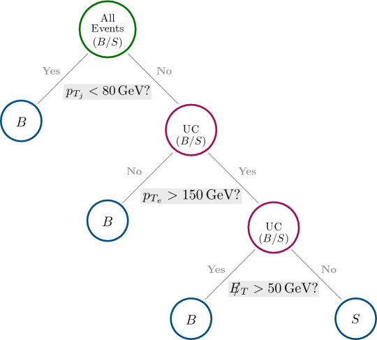
Figure 14: A simple 3-depth decision tree example, in which each note represents a cut based on the input parameters ($p_{T_{j}}$, $p_{T_{e}}$, and $E\!\!\!/_{T}$). “UC” standards of “unclassified” in the picture. Notice, this is only an illustration of a decision tree, and it is not reflecting the true classification result of our collider study.

The decision tree method is powerful but can be easily over-fitted, i.e, a tiny change in the input data set may result in large differences and inconsistencies in the classification results. To avoid this, a set of BDTs can be trained in a sequence such that the successive tree is created to minimize the error of the previous tree. Several sets of these can be trained and the final classification result is determined by the majority vote from all the BDTs. In this study, we use the AdaBoost (Adaptive Boost) to test a small part of the parameter space of our simplified model.

The details of the algorithm are described as follows. The $i-$th tree trained is called $T^{i}$, $W^{i}$ is its voting weight, and $w_{j}^{i}$ is the weight of the $j-$th sample in the $i-$th tree:

• The first tree ($T^{1}$) is trained such that all the samples have the same weight. Either the Gini or the entropy criteria can be used for this training. For each sample the tree predicts if the event is “signal-like” or “background-like”. The discrete output for each event is as follows:

  $$y_{j}^{i}=\left\{\begin{array}[]{cl}+1&\textrm{for signal-like events,}\\ -1&\textrm{for background-like events.}\end{array}\right.$$

• Each tree, $T^{i}$, has the voting weight $W^{i}$ which is defined as :

  $$W^{i}=\frac{1}{2}\log\left(\frac{1-\it err}{\it err}\right)$$ (52)

  with $\it err$ being the ratio of the misclassified samples to the total samples. A sample is misclassified if its prediction $y_{j}^{i}$ is different than the truth value $\hat{y}$, where $\hat{y}$ is 1 for signal events and -1 for background events. The voting weight is higher for trees with better classification. A small shift inside the logarithm will be added in practice to prevent infinity when error is 1 or 0.
  

• Subsequent trees ($T^{2}$, $T^{3}$, …, $T^{N}$) are generated. For each tree, $T^{i}$, that is trained, every sample is re-weighted depending on how it was classified. If the classification is correct, the sample weight is given as $w_{j}^{i}=w_{j}^{i-1}e^{-W^{i-1}}$. If the classification is incorrect then the sample weight is given by $w_{j}^{i}=w_{j}^{i-1}e^{W^{i-1}}$. After the training and the re-weighting, all weights ($w_{j}^{i}$) will be normalized meaning, for each tree the weights ($w_{j}^{i}$) will sum to 1.

• In each of the training, when certain samples are misidentified by the tree, they would be emphasized in the next tree due to the re-weighting. This is because, misidentified samples from the previous tree would have a higher weight in the next training, forcing the Gini or entropy criteria to classify them correctly.

• The process of tree training will end when a previously determined total number of trees $N$ has been reached.

• The final classification result, $y_{j}$ for the $j-$th sample is

  $$y_{j}=\frac{1}{N}\sum_{i=1}^{N}{y_{j}^{i}\,W^{i}}\ ,$$ (53)

  where $W^{i}$ is the voting weight of the $i-$th tree and $N$ is the total number of trees that are trained.

This BDT method is a powerful algorithm for signal-background classification however is very time consuming. This is because each tree must be generated sequentially and a completely new series of trees must be trained with new parameter choices for the simplified model. Given that we are interested in several different choices of masses and couplings in the model, we implement a different method described in the next section. This method allows us to build a classification model for the whole parameter space efficiently.

A.2 Recurrent Neural Network (RNN)

A neural network (NN) is a deep learning model comprising of a series of linear and non-linear transformations. The goal is to find an optimal set of parameters that transform a set of initial inputs to approximate the target. The idea is that this predictive model is made of connected units or nodes that mimic the neurons in the brain. The network consists of a series of layers that “learn” to classify the events as signal or background through transformations. The type of the layer and number of layers is defined by the network topology and is optimized to improve the classification. When we provide the network with a set of inputs, $x$, it passes through these layers, undergoing transformations, one after the other. The network then outputs its set of predictions $y$.

To improve the NN, one can define a loss function $\mathcal{L}(y,\hat{y})$, where $\hat{y}$ is the truth value and $y$ is the model output. As the NN becomes a better classifier, the predictions $(y)$ will get closer to the truth value $(\hat{y})$ hence reducing the loss. Hence one can optimize the parameters inside the NN by minimizing the loss function.

Usually, the inputs of a NN have fixed length. However, our simulations contain events with different numbers particles and the inputs do not have the same length. We can use a recurrent neural network (RNN) as our deep learning tool as it allows inputs of variable lengths using Gated Recurrent Units (GRUs) DBLP:journals/corr/ChoMGBSB14 ; DBLP:journals/corr/ChungGCB14 . A standard RNN has the property that the structure of the hidden layers will be updated when new inputs are provided and it also has the ability to “remember” parts of the previous input for optimized classification. This is depicted in Fig. 15.

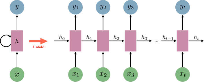
Figure 15: Visual representation of a standard RNN in folded version (left) and unfolded version (right). The sequence $\{x_{1},x_{2},x_{3},\ldots,x_{t}\}$ represents the input, $\{y_{1},y_{2},y_{3},\ldots,y_{t}\}$ represents the predicted output, and $\{h_{0},h_{1},h_{2},\ldots,h_{t}\}$ holds the information from the previous input. The graph illustrates that, at any given time $t$, the current layer will be updated with respect to a new input.

As stated before, we use this RNN to separate signal and background events. Kinematic properties of jets, electrons, and missing $E_{T}$ are used as inputs to three independent, recurrent networks. These are initially trained in parallel and then merged together into a fully connected sequential neural network. The described topology is depicted in Fig. 16. Based on the input variables, the network assigns a decision score ($d$) to every event. This score goes from $d=0$, indicating a perfectly-background-like event, indicating a perfectly-background-like event, to $d=1$, indicating a perfectly-signal-like event. We then determine a cutoff $d^{\ast}$ such that all events satisfying $d>d^{\ast}$ are classified as signal $S$ and the rest is background, maximizing the signal significance $S/\sqrt{S+B}$.

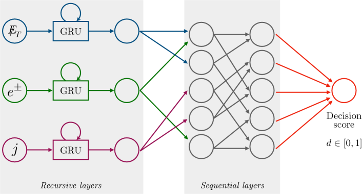
Figure 16: Visual representation of the Recurrent Neural Network (RNN) used in our study. The kinematic properties of jets, electrons, and missing energy are analyzed by independent Gated Recurrent Units (GRUs). The outcome is merged into a sequential neural network that produces a decision score $d$ between 0 and 1.

References

- (1) Particle Data Group collaboration, P. Zyla et al., Review of Particle Physics, PTEP 2020 (2020) 083C01.
- (2) Planck collaboration, N. Aghanim et al., Planck 2018 results. VI. Cosmological parameters, 1807.06209.
- (3) A. D. Sakharov, Violation of CP Invariance, C asymmetry, and baryon asymmetry of the universe, Pisma Zh. Eksp. Teor. Fiz. 5 (1967) 32–35.
- (4) M. Fukugita and T. Yanagida, Baryogenesis Without Grand Unification, Phys. Lett. B 174 (1986) 45–47.
- (5) S. Davidson and A. Ibarra, A Lower bound on the right-handed neutrino mass from leptogenesis, Phys. Lett. B 535 (2002) 25–32, [hep-ph/0202239].
- (6) KamLAND-Zen collaboration, A. Gando et al., Search for Majorana Neutrinos near the Inverted Mass Hierarchy Region with KamLAND-Zen, Phys. Rev. Lett. 117 (2016) 082503, [1605.02889].
- (7) nEXO collaboration, J. B. Albert et al., Sensitivity and Discovery Potential of nEXO to Neutrinoless Double Beta Decay, Phys. Rev. C 97 (2018) 065503, [1710.05075].
- (8) nEXO collaboration, S. A. Kharusi et al., nEXO Pre-Conceptual Design Report, 1805.11142.
- (9) LEGEND collaboration, N. Abgrall et al., The Large Enriched Germanium Experiment for Neutrinoless Double Beta Decay (LEGEND), AIP Conf. Proc. 1894 (2017) 020027, [1709.01980].
- (10) E. Armengaud et al., The CUPID-Mo experiment for neutrinoless double-beta decay: performance and prospects, Eur. Phys. J. C 80 (2020) 44, [1909.02994].
- (11) CUPID collaboration, W. R. Armstrong et al., CUPID pre-CDR, 1907.09376.
- (12) SNO+ collaboration, J. Paton, Neutrinoless Double Beta Decay in the SNO+ Experiment, in Prospects in Neutrino Physics, 3, 2019, 1904.01418.
- (13) F. F. Deppisch, J. Harz, M. Hirsch, W.-C. Huang and H. Päs, Falsifying High-Scale Baryogenesis with Neutrinoless Double Beta Decay and Lepton Flavor Violation, Phys. Rev. D 92 (2015) 036005, [1503.04825].
- (14) F. F. Deppisch, L. Graf, J. Harz and W.-C. Huang, Neutrinoless Double Beta Decay and the Baryon Asymmetry of the Universe, Phys. Rev. D 98 (2018) 055029, [1711.10432].
- (15) T. Li, X.-D. Ma and M. A. Schmidt, Implication of for generic neutrino interactions in effective field theories, Phys. Rev. D 101 (2020) 055019, [1912.10433].
- (16) F. F. Deppisch, K. Fridell and J. Harz, Constraining lepton number violating interactions in rare kaon decays, JHEP 12 (2020) 186, [2009.04494].
- (17) K. S. Babu and C. N. Leung, Classification of effective neutrino mass operators, Nucl. Phys. B 619 (2001) 667–689, [hep-ph/0106054].
- (18) A. de Gouvea and J. Jenkins, A Survey of Lepton Number Violation Via Effective Operators, Phys. Rev. D 77 (2008) 013008, [0708.1344].
- (19) D. V. Nanopoulos and S. Weinberg, Mechanisms for Cosmological Baryon Production, Phys. Rev. D 20 (1979) 2484.
- (20) E. W. Kolb and S. Wolfram, Baryon Number Generation in the Early Universe, Nucl. Phys. B 172 (1980) 224.
- (21) S. Davidson, E. Nardi and Y. Nir, Leptogenesis, Phys. Rept. 466 (2008) 105–177, [0802.2962].
- (22) W. Buchmuller, P. Di Bari and M. Plumacher, Leptogenesis for pedestrians, Annals Phys. 315 (2005) 305–351, [hep-ph/0401240].
- (23) G. Giudice, A. Notari, M. Raidal, A. Riotto and A. Strumia, Towards a complete theory of thermal leptogenesis in the SM and MSSM, Nucl. Phys. B 685 (2004) 89–149, [hep-ph/0310123].
- (24) G. Prezeau, M. Ramsey-Musolf and P. Vogel, Neutrinoless double beta decay and effective field theory, Phys. Rev. D 68 (2003) 034016, [hep-ph/0303205].
- (25) M. L. Graesser, An electroweak basis for neutrinoless double decay, JHEP 08 (2017) 099, [1606.04549].
- (26) P. Minkowski, at a Rate of One Out of Muon Decays?, Phys. Lett. B 67 (1977) 421–428.
- (27) T. Yanagida, Horizontal Symmetry and Masses of Neutrinos, Prog. Theor. Phys. 64 (1980) 1103.
- (28) S. L. Glashow, The Future of Elementary Particle Physics, NATO Sci. Ser. B 61 (1980) 687.
- (29) M. Gell-Mann, P. Ramond and R. Slansky, Complex Spinors and Unified Theories, Conf. Proc. C 790927 (1979) 315–321, [1306.4669].
- (30) R. N. Mohapatra and G. Senjanovic, Neutrino Masses and Mixings in Gauge Models with Spontaneous Parity Violation, Phys. Rev. D 23 (1981) 165.
- (31) S. Weinberg, Baryon and Lepton Nonconserving Processes, Phys. Rev. Lett. 43 (1979) 1566–1570.
- (32) F. F. Deppisch, J. Harz and M. Hirsch, Falsifying High-Scale Leptogenesis at the LHC, Phys. Rev. Lett. 112 (2014) 221601, [1312.4447].
- (33) A. Salvio, P. Lodone and A. Strumia, Towards leptogenesis at NLO: the right-handed neutrino interaction rate, JHEP 08 (2011) 116, [1106.2814].
- (34) B. Garbrecht, Why is there more matter than antimatter? Calculational methods for leptogenesis and electroweak baryogenesis, Prog. Part. Nucl. Phys. 110 (2020) 103727, [1812.02651].
- (35) A. Strumia, Baryogenesis via leptogenesis, in Les Houches Summer School on Theoretical Physics: Session 84: Particle Physics Beyond the Standard Model, pp. 655–680, 8, 2006, hep-ph/0608347.
- (36) M.-C. Chen, TASI 2006 Lectures on Leptogenesis, in Theoretical Advanced Study Institute in Elementary Particle Physics: Exploring New Frontiers Using Colliders and Neutrinos, 3, 2007, hep-ph/0703087.
- (37) CMS collaboration, S. Chatrchyan et al., A Search for a Doubly-Charged Higgs Boson in Collisions at TeV, Eur. Phys. J. C 72 (2012) 2189, [1207.2666].
- (38) ATLAS collaboration, M. Aaboud et al., Search for doubly charged Higgs boson production in multi-lepton final states with the ATLAS detector using proton–proton collisions at , Eur. Phys. J. C 78 (2018) 199, [1710.09748].
- (39) ATLAS collaboration, M. Aaboud et al., Search for heavy Majorana or Dirac neutrinos and right-handed gauge bosons in final states with two charged leptons and two jets at TeV with the ATLAS detector, JHEP 01 (2019) 016, [1809.11105].
- (40) CMS collaboration, S. Chatrchyan et al., Search for Top Squarks in -Parity-Violating Supersymmetry using Three or More Leptons and B-Tagged Jets, Phys. Rev. Lett. 111 (2013) 221801, [1306.6643].
- (41) F. Najafi, J. Kumar and D. London, CP violation in rare lepton-number-violating decays at the LHC, JHEP 04 (2021) 021, [2011.03686].
- (42) CMS collaboration, V. Khachatryan et al., Search for new physics in same-sign dilepton events in proton–proton collisions at , Eur. Phys. J. C 76 (2016) 439, [1605.03171].
- (43) CMS collaboration, A. M. Sirunyan et al., Search for physics beyond the standard model in events with two leptons of same sign, missing transverse momentum, and jets in proton–proton collisions at , Eur. Phys. J. C 77 (2017) 578, [1704.07323].
- (44) ATLAS collaboration, M. Aaboud et al., Search for low-mass resonances decaying into two jets and produced in association with a photon using collisions at TeV with the ATLAS detector, Phys. Lett. B 795 (2019) 56–75, [1901.10917].
- (45) ATLAS collaboration, G. Aad et al., Search for new resonances in mass distributions of jet pairs using 139 fb-1 of collisions at TeV with the ATLAS detector, JHEP 03 (2020) 145, [1910.08447].
- (46) CMS collaboration, Search for new physics in the lepton plus missing transverse momentum final state in proton-proton collisions at 13 TeV center-of-mass energy, .
- (47) S. Banerjee, B. Bhattacherjee, A. Goudelis, B. Herrmann, D. Sengupta and R. Sengupta, Determining the lifetime of long-lived particles at the HL-LHC, Eur. Phys. J. C 81 (2021) 172, [1912.06669].
- (48) A. Alloul, N. D. Christensen, C. Degrande, C. Duhr and B. Fuks, FeynRules 2.0 - A complete toolbox for tree-level phenomenology, Comput. Phys. Commun. 185 (2014) 2250–2300, [1310.1921].
- (49) J. Alwall, R. Frederix, S. Frixione, V. Hirschi, F. Maltoni, O. Mattelaer et al., The automated computation of tree-level and next-to-leading order differential cross sections, and their matching to parton shower simulations, JHEP 07 (2014) 079, [1405.0301].
- (50) T. Sjöstrand, S. Ask, J. R. Christiansen, R. Corke, N. Desai, P. Ilten et al., An Introduction to PYTHIA 8.2, Comput. Phys. Commun. 191 (2015) 159–177, [1410.3012].
- (51) DELPHES 3 collaboration, J. de Favereau, C. Delaere, P. Demin, A. Giammanco, V. Lemaître, A. Mertens et al., DELPHES 3, A modular framework for fast simulation of a generic collider experiment, JHEP 02 (2014) 057, [1307.6346].
- (52) T. Peng, M. J. Ramsey-Musolf and P. Winslow, TeV lepton number violation: From neutrinoless double- decay to the LHC, Phys. Rev. D 93 (2016) 093002, [1508.04444].
- (53) Physics at the FCC-hh, a 100 TeV pp collider, 1710.06353.
- (54) J. Tang et al., Concept for a Future Super Proton-Proton Collider, 1507.03224.
- (55) M. Selvaggi, A Delphes parameterisation of the FCC-hh detector, Tech. Rep. CERN-FCC-PHYS-2020-0003, CERN, Geneva, May, 2020.
- (56) M. Paganini, An Introduction to Deep Learning with Keras. 2nd Developers@CERN Forum, .
- (57) D. Guest, J. Collado, P. Baldi, S.-C. Hsu, G. Urban and D. Whiteson, Jet Flavor Classification in High-Energy Physics with Deep Neural Networks, Phys. Rev. D 94 (2016) 112002, [1607.08633].
- (58) L. Bradshaw, R. K. Mishra, A. Mitridate and B. Ostdiek, Mass Agnostic Jet Taggers, SciPost Phys. 8 (2020) 011, [1908.08959].
- (59) A. Alves, Stacking machine learning classifiers to identify Higgs bosons at the LHC, JINST 12 (2017) T05005, [1612.07725].
- (60) ATLAS collaboration, A. Buzatu. Machine Learning for Higgs boson physics at the LHC.
- (61) D. Curtin, J. Galloway and J. G. Wacker, Measuring the coupling from same-sign dilepton measurements, Phys. Rev. D 88 (2013) 093006, [1306.5695].
- (62) E. Izaguirre and B. Shuve, Multilepton and Lepton Jet Probes of Sub-Weak-Scale Right-Handed Neutrinos, Phys. Rev. D 91 (2015) 093010, [1504.02470].
- (63) C. O. Dib, C. Kim, K. Wang and J. Zhang, Distinguishing Dirac/Majorana Sterile Neutrinos at the LHC, Phys. Rev. D 94 (2016) 013005, [1605.01123].
- (64) M. Nemevšek, F. Nesti and J. C. Vasquez, Majorana Higgses at colliders, JHEP 04 (2017) 114, [1612.06840].
- (65) G. Li. Private communication, March, 2021.
- (66) J. C. Helo, H. Li, N. A. Neill, M. Ramsey-Musolf and J. C. Vasquez, Probing neutrino Dirac mass in left-right symmetric models at the LHC and next generation colliders, Phys. Rev. D 99 (2019) 055042, [1812.01630].
- (67) J. Pan, J.-H. Chen, X.-G. He, G. Li and J.-Y. Su, Triply charged Higgs bosons at a 100 TeV collider, 1909.07254.
- (68) M. Muskinja, Search for new physics processes with same charge leptons in the final state with the ATLAS detector using proton–proton collisions at TeV. Iskanje procesov nove fizike s pari enako nabitih leptonov v končnem stanju z detektorjem ATLAS s trki protonov pri energiji TeV, Aug, 2018.
- (69) V. Cirigliano, W. Dekens, J. de Vries, M. L. Graesser and E. Mereghetti, A neutrinoless double beta decay master formula from effective field theory, JHEP 12 (2018) 097, [1806.02780].
- (70) J. Donoghue, E. Golowich and B. Holstein, Dynamics of the Standard Model (Second Edition), Dynamics of the Standard Model (Second Edition) Cambridge Univ. Press (2014) .
- (71) V. Cirigliano, W. Dekens, M. Graesser and E. Mereghetti, Neutrinoless double beta decay and chiral , Phys. Lett. B 769 (2017) 460–464, [1701.01443].
- (72) A. Nicholson et al., Heavy physics contributions to neutrinoless double beta decay from QCD, Phys. Rev. Lett. 121 (2018) 172501, [1805.02634].
- (73) A. Faessler, S. Kovalenko and F. Simkovic, Pions in nuclei and manifestations of supersymmetry in neutrinoless double beta decay, Phys. Rev. D 58 (1998) 115004, [hep-ph/9803253].
- (74) J. Hyvärinen and J. Suhonen, Nuclear matrix elements for decays with light or heavy Majorana-neutrino exchange, Phys. Rev. C 91 (2015) 024613.
- (75) V. Cirigliano, W. Dekens, J. De Vries, M. L. Graesser, E. Mereghetti, S. Pastore et al., New Leading Contribution to Neutrinoless Double- Decay, Phys. Rev. Lett. 120 (2018) 202001, [1802.10097].
- (76) E. J. Chun et al., Probing Leptogenesis, Int. J. Mod. Phys. A 33 (2018) 1842005, [1711.02865].
- (77) S. M. Bilenky and S. T. Petcov, Nuclear matrix elements of 0 nu beta beta decay: Possible test of the calculations, hep-ph/0405237.
- (78) F. Deppisch and H. Pas, Pinning down the mechanism of neutrinoless double beta decay with measurements in different nuclei, Phys. Rev. Lett. 98 (2007) 232501, [hep-ph/0612165].
- (79) V. M. Gehman and S. R. Elliott, Multiple-Isotope Comparison for Determining 0 nu beta beta Mechanisms, J. Phys. G 34 (2007) 667–678, [hep-ph/0701099].
- (80) S. Dell’Oro, S. Marcocci, M. Viel and F. Vissani, The contribution of light Majorana neutrinos to neutrinoless double beta decay and cosmology, JCAP 12 (2015) 023, [1505.02722].
- (81) M. T. Frandsen, C. Hagedorn, W.-C. Huang, E. Molinaro and H. Päs, Asymmetric dark matter, baryon asymmetry and lepton number violation, Phys. Lett. B 782 (2018) 387–394, [1801.09314].
- (82) A. Hoecker, P. Speckmayer, J. Stelzer, J. Therhaag, E. von Toerne, H. Voss et al., TMVA-toolkit for multivariate data analysis, physics/0703039.
- (83) D. Guest, K. Cranmer and D. Whiteson, Deep Learning and its Application to LHC Physics, Ann. Rev. Nucl. Part. Sci. 68 (2018) 161–181, [1806.11484].
- (84) K. Cho, B. van Merrienboer, Ç. Gülçehre, F. Bougares, H. Schwenk and Y. Bengio, Learning phrase representations using RNN encoder-decoder for statistical machine translation, CoRR abs/1406.1078 (2014) , [1406.1078].
- (85) J. Chung, Ç. Gülçehre, K. Cho and Y. Bengio, Empirical evaluation of gated recurrent neural networks on sequence modeling, CoRR abs/1412.3555 (2014) , [1412.3555].