Two-Stream Consensus Network: Submission to HACS Challenge 2021 Weakly-Supervised Learning Track

Abstract

This technical report presents our solution to the HACS Temporal Action Localization Challenge 2021, Weakly-Supervised Learning Track. The goal of weakly-supervised temporal action localization is to temporally locate and classify action of interest in untrimmed videos given only video-level labels. We adopt the two-stream consensus network (TSCN) [5] as the main framework in this challenge. The TSCN consists of a two-stream base model training procedure and a pseudo ground truth learning procedure. The base model training encourages the model to predict reliable predictions based on single modality (, RGB or optical flow), based on the fusion of which a pseudo ground truth is generated and in turn used as supervision to train the base models. On the HACS v1.1.1 dataset, without fine-tuning the feature-extraction I3D models, our method achieves $22.20\%$ on the validation set and $21.68\%$ on the testing set in terms of average mAP. Our solution ranked the 2nd in this challenge, and we hope our method can serve as a baseline for future academic research.

1 Our Solution

We adopt the two-stream consensus network (TSCN) [5] as the main framework. It consists of two main procedures: two-stream base model training and pseudo ground truth learning. Figure 1 shows the framework of our method.

1.1 Feature Extraction

We construct our model upon snippet-level feature sequences extracted from the raw video volume. The RGB and optical flow features are extracted with pre-trained I3D [1]) from non-overlapping fixed-length RGB frame snippets and optical flow snippets, respectively. Formally, given a video with $T$ non-overlapping snippets, we denote the RGB features and optical flow features as $\{\mathbf{f}_{\text{RGB},i}\}_{i=1}^{T}$ and $\{\mathbf{f}_{\text{flow},i}\}_{i=1}^{T}$, respectively, where $\mathbf{f}_{\text{RGB},i},\mathbf{f}_{\text{flow},i}\in\mathbb{R}^{D}$ are the feature representations of the $i$-th RGB frame and optical flow snippet, respectively, and $D$ represents the channel dimension.

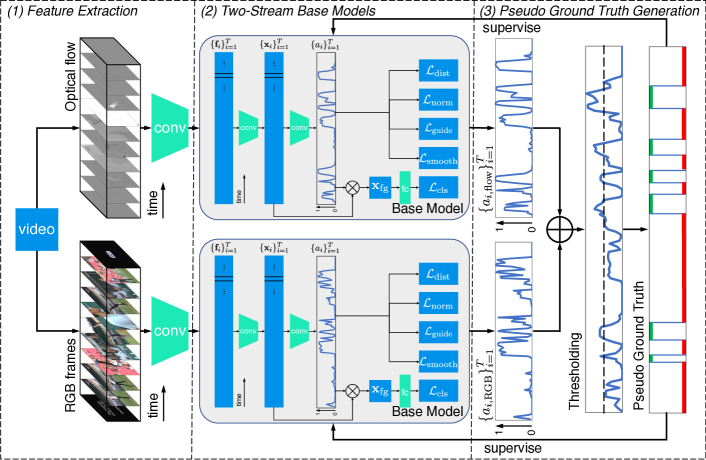
Figure 1: An overview of the Two-Stream Consensus Network, which consists of three parts: (1) feature extraction, where RGB and optical flow snippet-level features are pre-extracted; (2) two-stream base models, where action recognition is performed on the two modalities with two-stream base models, respectively; (3) pseudo ground truth generation, where a frame-level pseudo ground truth is generated from the two-stream late-fusion attention sequence and in turn provides frame-level supervision to two-stream base models.

1.2 Two-Stream Base Models

After obtaining the RGB and optical flow features, we first use two-stream base models to perform the video-level action classification. The features of two modalities are fed into two separate base models, respectively, and the two base models use the same architecture but do not share parameters. Therefore, we omit the subscript RGB and flow to denote a general operation for both modalities.

To embed the extracted features to task-specific space, we use a single temporal convolutional layer with a kernel size $3$ to embed the input feature, and generate a set of new features $\{\mathbf{x}_{i}\}_{i=1}^{T}$, where $\mathbf{x}_{i}\in\mathbb{R}^{D}$.

As a video may contain background snippets, to perform video-level classification, we need to select snippets that are likely to contain action instances and meanwhile filter out snippets that are likely to contain background. To this end, an attention value $a_{i}\in(0,1)$ to measure the likelihood of the $i$-th snippet containing an action is given by a fully-connected (FC) sigmoid layer. We then perform attention-weighted pooling over the feature sequence to generate a single foreground feature $\mathbf{x}_{\text{fg}}$, and feed it to an FC softmax layer to get the video-level prediction:

$$\mathbf{x}_{\text{fg}}=\frac{1}{\sum_{i=1}^{T}a_{i}}\sum_{i=1}^{T}a_{i}\mathbf{x}_{i},$$ (1)

$$\hat{y}_{c}=\frac{e^{\mathbf{w}_{c}\cdot\mathbf{x}_{\text{fg}}+b_{c}}}{\sum_{i=1}^{C}e^{\mathbf{w}_{i}\cdot\mathbf{x}_{\text{fg}}+b_{i}}},$$ (2)

where $\hat{y}_{c}$ is the probability that the video contains the $c$-th action, and $\mathbf{w}_{c}$ and $b_{c}$ are the weight and bias of the FC layer for category $c$, respectively. The classification loss function $\mathcal{L}_{\text{cls}}$ is defined as the standard binary cross entropy loss.

In addition, the temporal-class activation map (T-CAM) $\{\textbf{s}_{i}\}_{i=1}^{T}$, $\textbf{s}_{i}\in\mathbb{R}^{C}$ is also generated by sliding the classification FC softmax layer over all snippet features:

$$s_{i,c}=\frac{e^{\mathbf{w}_{c}\cdot\mathbf{x}_{i}+b_{c}}}{\sum_{j=1}^{C}e^{\mathbf{w}_{j}\cdot\mathbf{x}_{i}+b_{j}}},$$ (3)

where $s_{i,c}$ is the T-CAM value of $i$-th snippet for category $c$.

For better attention and T-CAM learning, we further adopt a smooth loss, the attention normalization loss [5], a distinctness loss, and a variant of the self-guided attention loss [2] in the base model training.

The smooth loss enforces temporally proximate snippets to give similar attention predictions, and thus helps generate a more smooth attention sequence:

$$\mathcal{L}_{\text{smooth}}=\frac{1}{T-1}\sum_{t=1}^{T-1}|a_{t}-a_{t+1}|$$ (4)

The attention normalization loss [5] maximizes the difference between the average top-$l$ attention values and the average bottom-$l$ attention values, and forces the foreground attention to be $1$ and background attention to be $0$:

$$\mathcal{L}_{\text{norm}}=\frac{1}{l}\min_{\begin{subarray}{c}a\subset\{a_{i}\}\\ |a|=l\end{subarray}}\sum_{\phi\in a}\phi-\frac{1}{l}\max_{\begin{subarray}{c}a\subset\{ai\}\\ |a|=l\end{subarray}}\sum_{\phi\in a}\phi,$$ (5)

where $l=\max\left(1,\lfloor\frac{T}{k}\rfloor\right)$ and $k$ is a hyperparameter to control the selected snippets.

The distinctness loss $\mathcal{L}_{\text{dist}}$ encourages the foreground feature $\mathbf{x}_{\text{fg}}$ and background feature $\mathbf{x}_{\text{bg}}$ to be distinct in the feature space:

$$\mathcal{L}_{\text{dist}}=\max\left(0,\frac{\mathbf{x}_{\text{fg}}\cdot\mathbf{x}_{\text{bg}}}{\|\mathbf{x}_{\text{fg}}\|\|\mathbf{x}_{\text{bg}}\|}-m\right),$$ (6)

where $\|\cdot\|$ is the L2 norm, and $m$ is a hyperparameter empirically set to $0.5$.

The self-guided attention loss [2] pursues a consensus between the bottom-up attention and the top-down T-CAM. In our method, as we do not exploit the background classification, we discard the background modeling term in the original guide loss. Besides, we empirically observe that the attention tends to produce more reliable activations than the T-CAM, and thus we detach the gradient for the attention in the guide loss. The guide loss variant employed in our method is formulated as:

$$\mathcal{L}_{\text{guide}}=\frac{1}{T}\sum_{i=1}^{T}|\text{sg}(a_{i})-s_{i,c^{*}}|,$$ (7)

where $\text{sg}(\cdot)$ denotes stop gradient, and $c^{*}$ is the ground truth action class.

The overall loss for the base model training is a weighted sum of the loss terms:

$$\mathcal{L}_{\text{base}}=\mathcal{L}_{\text{cls}}+\lambda_{1}\mathcal{L}_{\text{smooth}}+\lambda_{2}\mathcal{L}_{\text{norm}}+\lambda_{3}\mathcal{L}_{\text{dist}}+\lambda_{4}\mathcal{L}_{\text{guide}},$$ (8)

where $\lambda_{1}$, $\lambda_{2}$, $\lambda_{3}$ and $\lambda_{4}$ are weight parameters.

1.3 Pseudo Ground Truth Learning

We iteratively refine the two-stream base models with a frame-level pseudo ground truth, which is generated by two-stream prediction fusion. Specifically, we divide the whole training process into several refinement iterations. At refinement iteration $0$, only video-level labels are used for training. And at refinement iteration $n+1$, a frame-level pseudo ground truth is generated at refinement iteration $n$, and provides frame-level supervision for the current refinement iteration.

Speficially, we use the fusion attention sequence $\{a_{\text{fuse},i}^{(n)}\}_{i=1}^{T}$ at refinement iteration $n$ to generate pseudo ground truth $\{\mathcal{G}_{i}^{(n+1)}\}_{i=1}^{T}$ for refinement iteration $n+1$, where $a_{\text{fuse},i}^{(n)}=\beta a_{\text{RGB},i}^{(n)}+(1-\beta)a_{\text{flow},i}^{(n)}$, and $\beta\in[0,1]$ is a hyperparameter to control the relative importance of RGB and flow attentions.

The pseudo ground truth thresholds the attention sequence to generate a binary sequence:

$$\mathcal{G}_{i}^{(n+1)}=\left\{\begin{array}[]{lr}1,\quad a_{\text{fuse},i}^{(n)}>\theta;&\\ 0,\quad a_{\text{fuse},i}^{(n)}\leq\theta,&\\ \end{array}\right.$$ (9)

where $\theta$ is the threshold value.

After obtaining the frame-level pseudo ground truth, we force the attention sequence generated by each stream to be similar to the pseudo ground truth with a binary cross entropy loss:

$$\mathcal{L}_{\text{pseudo}}^{(n+1)}= -\frac{1}{T}\sum_{i=1}^{T}\mathcal{G}_{i}^{(n+1)}\log\left(a_{i}^{(n+1)}\right)+$$ (10)

$$\left(1-\mathcal{G}_{i}^{(n+1)}\right)\log\left(1-a_{i}^{(n+1)}\right)$$

At refinement iteration $n+1$, the total loss for each stream is

$$\mathcal{L}_{\text{total}}^{(n+1)}=\mathcal{L}_{\text{cls}}+\lambda_{3}\mathcal{L}_{\text{dist}}+\lambda_{4}\mathcal{L}_{\text{guide}},+\lambda_{5}\mathcal{L}_{\text{pseudo}}^{(n+1)},$$ (11)

where $\lambda_{5}$ is a hyperparameter to control the relative importance of two losses. Note that we remove the attention normalization loss and in the pseudo ground truth learning, as the loss term assumes at least $\frac{1}{k}$ and $\frac{1}{k}$ of each video are actions and backgrounds, respectively. However, it does not always hold (some videos do not contain background), and will bring noise for the pseudo ground truth learning. The smooth loss is also removed as it leads to trivial solution where all videos are actions without the supervision the attention normalization loss.

1.4 Action Localization

During testing, we first temporally upsample the attention sequence and T-CAM by a factor of $8$ via linear interpolation. Then, we select top-$2$ action categories from the fusion video-level prediction $\hat{\textbf{y}}_{\text{fuse}}$ to perform action localization, where $\hat{\textbf{y}}_{\text{fuse}}=\beta\hat{\textbf{y}}_{\text{RGB}}+(1-\beta)\hat{\textbf{y}}_{\text{flow}}$. Action proposals are generated by progressively thresholding the attention sequence from $0$ to $1.0$, with a step size of $0.025$, and concatenating proximate snippets. The action proposals are scored following TSCN [5]. Formally, given action proposal $(t_{s},t_{e},c)$, fusion attention $\{a_{\text{fuse},i}\}_{i=1}^{T}$ and T-CAM $\{\textbf{s}_{\text{fuse},i}\}_{i=1}^{T}$, where $\textbf{s}_{\text{fuse},i}=\beta\textbf{s}_{\text{RGB},i}+(1-\beta)\textbf{s}_{\text{flow},i}$, the score $\psi$ is computed as

$$\psi= \frac{\sum_{i=t_{s}}^{t_{e}}a_{\text{fuse},i}s_{\text{fuse},i,c}}{t_{e}-t_{s}}-$$ (12)

$$\frac{\sum_{i=T_{s}}^{T_{e}}a_{\text{fuse},i}s_{\text{fuse},i,c}-\sum_{i=t_{s}}^{t_{e}}a_{\text{fuse},i}s_{\text{fuse},i,c}}{T_{e}-T_{s}-(t_{e}-t_{s})},$$

where $T_{s}=t_{s}-\frac{L}{4}$, $T_{e}=t_{e}+\frac{L}{4}$, and $L=t_{e}-t_{s}$. We finally use NMS with IoU threshold $0.6$ to filter out redundant detections.

2 Experiments and Discussions

2.1 Implementation Details

The optical flow is estimated via the TV-L1 algorithm [4]. The feature-extraction backbone I3D [1] is pre-trained on the Kinetics dataset [1], and is not fine-tuned on the HACS dataset [6]. In this competition, we use the off-the-shelf $2$ FPS RGB snippet-level features provided by the dataset [6], and extract the optical flow features with a snippet length of $16$ frames. The majority of the hyperparameters are set according to [2, 5]: $\lambda_{1}=\lambda_{2}=\lambda_{4}=0.1$, $k=8$, and $\theta=0.5$. Other hyperparameters are set according to a grid search: $\beta=0.6$, $\lambda_{3}=0.1$ and $\lambda_{5}=0.01$. We use the AdamW optimizer with a fixed learning rate $0.0005$. We train the model for a total of $5$ refinement iterations, with each refinement iteration contains $10$ epochs. At each refinement iteration, we simply select the latest model from the last refinement iteration to generate the pseudo ground truth.

Table 1: Single-stream performance with different loss combinations on the HACS validation set.

$\mathcal{L}_{\text{cls}}$	$\mathcal{L}_{\text{smooth}}$	$\mathcal{L}_{\text{norm}}$	$\mathcal{L}_{\text{dist}}$	$\mathcal{L}_{\text{guide}}$	mAP@IoU (%)
					0.5	0.75	0.95	Avg
✓	-	-	-	-	9.23	4.45	1.12	5.03
✓	✓	-	-	-	17.53	11.41	4.54	11.69
✓	✓	✓	-	-	25.82	15.77	5.42	16.33
✓	✓	✓	✓	-	26.54	16.18	5.50	16.86
✓	✓	✓	✓	✓	27.46	17.19	6.26	17.69

(a) RGB stream-only localization performance.

$\mathcal{L}_{\text{cls}}$	$\mathcal{L}_{\text{smooth}}$	$\mathcal{L}_{\text{norm}}$	$\mathcal{L}_{\text{dist}}$	$\mathcal{L}_{\text{guide}}$	mAP@IoU (%)
					0.5	0.75	0.95	Avg
✓	-	-	-	-	5.60	2.17	0.19	2.63
✓	✓	-	-	-	14.47	9.43	3.40	9.64
✓	✓	✓	-	-	19.08	11.73	4.75	12.31
✓	✓	✓	✓	-	19.24	11.84	4.83	12.40
✓	✓	✓	✓	✓	19.57	12.17	4.90	12.74

(b) Flow stream-only localization performance.

Table 2: Performance w/ pseudo ground truth learning in different refinement iterations on the HACS validation and testing sets.

	Modality	Validation				Test
		0.5	0.75	0.95	Avg	Avg
0	RGB	27.46	17.19	6.26	17.69	-
	Flow	19.57	12.17	4.90	12.74	-
	Fusion	29.91	18.50	6.99	19.12	18.75
1	RGB	26.85	16.98	6.27	17.38	-
	Flow	23.57	13.86	5.27	14.74	-
	Fusion	31.30	19.14	6.96	19.83	-
2	RGB	30.45	18.42	6.39	19.16	-
	Flow	24.09	14.39	5.43	15.16	-
	Fusion	33.47	20.03	6.81	20.91	20.30
3	RGB	32.62	19.32	6.36	20.18	-
	Flow	23.21	13.97	4.82	14.58	-
	Fusion	35.07	20.85	6.87	21.82	-
4	RGB	33.54	19.57	6.17	20.54	-
	Flow	23.12	13.74	4.50	14.38	-
	Fusion	35.43	20.94	6.80	21.93	21.33

2.2 Results

Two-stream base models. The performance of two-stream base models w/o pseudo ground truth supervision is reported in Table 1, where different combinations of loss terms are evaluated. The results show the addition of each loss contributes to the performance improvement.

Pseudo ground truth learning. Table 2 reports the performance changes in different refinement iterations. The results reveal that pseudo ground truth consistently improves the fusion results, and eventually saturates at the $3$-rd and $4$-th refinement iterations. The pseudo ground truth also greatly improves the single-stream models. Specifically, it improves the performance of the RGB model from $17.69\%$ to $20.54\%$ in terms of average mAP, and improves the performance of the flow model from $12.74\%$ to $15.16\%$.

Exponential moving average emsemble. Inspired by the mean teacher [3], after the pseudo ground truth learning, we ensemble the models from all $5$ refinement iterations by exponentially moving average their parameters with a successive weight $0.2$. The final ensemble model achieves $22.20\%$ average mAP on the HACS validation set, and $21.68\%$ on the HACS testing set.

References

- [1] Joao Carreira and Andrew Zisserman. Quo vadis, action recognition? a new model and the kinetics dataset. In CVPR, pages 6299–6308, 2017.
- [2] Phuc Xuan Nguyen, Deva Ramanan, and Charless C Fowlkes. Weakly-supervised action localization with background modeling. In ICCV, pages 5502–5511, 2019.
- [3] Antti Tarvainen and Harri Valpola. Mean teachers are better role models: Weight-averaged consistency targets improve semi-supervised deep learning results. arXiv preprint arXiv:1703.01780, 2017.
- [4] Christopher Zach, Thomas Pock, and Horst Bischof. A duality based approach for realtime tv-l 1 optical flow. In PR, pages 214–223, 2007.
- [5] Yuanhao Zhai, Le Wang, Wei Tang, Qilin Zhang, Junsong Yuan, and Gang Hua. Two-stream consensus network for weakly-supervised temporal action localization. In ECCV, pages 37–54, 2020.
- [6] Hang Zhao, Antonio Torralba, Lorenzo Torresani, and Zhicheng Yan. Hacs: Human action clips and segments dataset for recognition and temporal localization. In ICCV, pages 8668–8678, 2019.