Lossy Compression for Lossless Prediction

Abstract

Most data is automatically collected and only ever “seen” by algorithms. Yet, data compressors preserve perceptual fidelity rather than just the information needed by algorithms performing downstream tasks. In this paper, we characterize the bit-rate required to ensure high performance on all predictive tasks that are invariant under a set of transformations, such as data augmentations. Based on our theory, we design unsupervised objectives for training neural compressors. Using these objectives, we train a generic image compressor that achieves substantial rate savings (more than $1000\times$ on ImageNet) compared to JPEG on 8 datasets, without decreasing downstream classification performance.

1 Introduction

Progress in important areas requires processing huge amounts of data. For climate prediction, models are still data-limited [1], despite the Natl. Center for Computational Sciences storing 32 million gigabytes (GB) of climate data [2]. For autonomous driving, capturing a realistic range of rare events with current methods requires around 3 trillion GB of data. At these scales, data are only processed by task-specific algorithms, and storing data in human-readable formats can be prohibitive. We need compressors that retain only the information needed for algorithmic execution of downstream tasks.

(a) Source

(b) Standard rec.

(c) Our rec.

Figure 0: Our unsupervised coder improves compression by only keeping information necessary for typical tasks. (left) source augmented MNIST digit; (center) a neural perceptual compressor achieves 130 bit-rate; (right) our invariant compressor achieves 48 bit-rate.

Existing lossy compressors are not up to the challenge, because they aim to reconstruct the data for human perception [5, 6, 7, 8, 9, 10]. However, much of perceptual information is not needed to perform the tasks that we care about. Consider classifying images, which can require about 1 MB to store. Classification is typically invariant under small image transformations, such as rescalings or rotations, and could instead be performed using a representation that discards such information (see Fig. 1). The amount of unnecessary perceptual information is likely substantial, as illustrated by the fact that typical image classification can be performed using a detailed caption, which requires only about 1 kB to store ($1000\times$ fewer bits).

Our goal is to quantify the bit-rate needed to ensure high performance on a collection of prediction tasks. In the simple case of a single supervised task, the minimum bit-rate is achieved by compressing predicted labels, and essentially corresponds to the Information Bottleneck (IB; [11]). Our challenge, instead, is to ensure good performance on any future tasks of interest, which will rarely be completely known at compression time, or might be too large to enumerate.

We overcome this challenge by focusing on sets of tasks that are invariant under user-defined transformations (e.g., translation, brightness, cropping), as is the case for many tasks of interest to humans [12, 13]. This structure allows us to characterize a worst-case invariant task, which bounds the relative predictive performance on all invariant tasks. As a result, the bit-rate required to perform well on all invariant tasks is exactly the rate to compress the worst-case labels. At a high level, the worst-case task is to recognize which examples are transformed versions of one another, and rate savings come from discarding information from those transformations.

We also provide two unsupervised neural compressors to target the optimal rates. One is similar to a variational autoencoder [14] that reconstructs canonical examples (Fig. 1). Our second is a simple modification of contrastive self-supervised learning (SSL; [15]), which allows us to convert pre-trained SSL models into powerful, generic compressors. Our contributions are:

• We formalize the notion of compression for downstream predictive tasks.

• We characterize the bits needed for high performance on any task invariant to augmentations.

• We provide unsupervised objectives to train compressors that approximate the optimal rates.

• We show that our compressor outperforms JPEG by orders of magnitude on 8 datasets on which it was never trained (i.e., zero-shot). E.g., on ImageNet [16], it decreases the bit-rate by $1000\times$.

2 Rate-distortion theory background

The goal of lossy compression theory is to find the number of bits (bit-rate) required to store outcomes $x$ of a random variable (r.v.) $X$, so that it can be reconstructed within a certain tolerance. This is accomplished in Shannon’s [17] rate-distortion (RD) theory by mapping $X$ into a r.v. $Z$ with low mutual information $\operatorname{I}\negthinspace\left[X;Z\right]$. Specifically, given a distortion measure $\operatorname{D}\negthinspace\left[X,Z\right]$, the RD theory characterizes the minimal achievable bit-rate for a distortion threshold $\delta$ by

$$Rate(\delta)=\min_{p(Z|X)}\operatorname{I}\negthinspace\left[X;Z\right]\quad\text{such that}\quad\operatorname{D}\negthinspace\left[X,Z\right]\leq\delta\,.$$ (1)

In lossy compression, $Z$ is usually a reconstruction of $X$, i.e., it aims to faithfully approximate $X$. As a result, typical distortions, e.g., the mean squared error (MSE), assume that the sample spaces $\mathcal{X},\mathcal{Z}$ of both r.v.s are the same. This assumption is not required. Indeed, any distortion $d:\mathcal{X}\times\mathcal{Z}\to\mathbb{R}_{\geq 0}$ of the form $\operatorname{D}\negthinspace\left[X,Z\right]=\operatorname{E}_{p(X,Z)}\negthinspace\left[d(X,Z)\right]$, where there exists a $z\in Z$ such that $\operatorname{D}\negthinspace\left[X,z\right]$ is finite, is a valid choice [18]. This shows that RD theory can be used outside of reconstructions. In the following we refer to $Z$ as a compressed representation of $X$ to distinguish it from a reconstruction.

3 Minimal bit-rate for high predictive performance

In this section, we characterize the bit-rate needed to represent $X$ to ensure high performance on downstream tasks. Our argument has three high-level steps: 1 define a distortion that controls downstream performance when predicting from $Z$ instead of $X$; 2 simplify and validate this distortion when desired tasks satisfy an invariance condition; 3 apply RD theory with the valid distortion. For simplicity, our presentation is relatively informal; formal proofs are in Apps. A and B.

3.1 A distortion for worst-case predictive performance

Suppose $X$ is an image. Potential downstream tasks might include $Y_{\text{dog}}$, whether the image displays a dog; or $Y_{\text{hd}}$, whether the image is hand-drawn. Formally, these and other downstream tasks are expressed as $\mathcal{T}=\negthinspace\left\{Y_{\text{dog}},Y_{\text{hd}},\ldots\right\}$, a set of random variables that are jointly distributed with $X$. Let $\operatorname{R}\negthinspace\left[Y\,|\,X\right]$ denote the Bayes (best possible) risk when predicting $Y$ from $X$. For ease of presentation in the main paper, we consider only classification tasks $\mathcal{T}$ and Bayes risk of the standard log loss $\operatorname{R}\negthinspace\left[Y\,|\,X\right]\vcentcolon=\inf_{q}\operatorname{E}_{p(X,Y)}\negthinspace\left[-\log q(Y|X)\right]$. We deal with MSE and regression in Sec. B.6.

In this setting, a meaningful distortion $\operatorname{D_{\scriptscriptstyle\mathcal{T}}}\negthinspace\left[X,Z\right]{}$ quantifies the difference between predicting any $Y\in\mathcal{T}$ from the compressed $Z$, as opposed to using $X$. This is the worst-case excess risk,

$$\operatorname{D_{\scriptscriptstyle\mathcal{T}}}\negthinspace\left[X,Z\right]{}\vcentcolon=\sup_{Y\in\mathcal{T}{}}\quad\operatorname{R}\negthinspace\left[Y\,|\,Z\right]-\operatorname{R}\negthinspace\left[Y\,|\,X\right].$$ (2)

If $\operatorname{D_{\scriptscriptstyle\mathcal{T}}}\negthinspace\left[X,Z\right]{}=0$, it is possible to achieve lossless prediction: performing as well using $Z$ as using $X$. More generally, bounding $\mathrm{D}_{\scriptscriptstyle\mathcal{T}}$ by $\delta$ ensures that $\operatorname{R}\negthinspace\left[Y\,|\,Z\right]-\operatorname{R}\negthinspace\left[Y\,|\,X\right]\leq\delta$ for all tasks in $\mathcal{T}$. However, there are two issues that need to be addressed before Eq. 2 can be used. First, it is not clear whether $\mathrm{D}_{\scriptscriptstyle\mathcal{T}}$ is a valid distortion for RD theory. Second, the worst excess-risk $\mathrm{D}_{\scriptscriptstyle\mathcal{T}}$ assumes access to all downstream tasks of interest $\mathcal{T}{}$ during compression, which is unrealistic in general.

3.2 Invariant tasks

The tasks that we care about are not arbitrary, and often share structure. One such structure is invariance to certain pre-specified transformations of input data. For example, computer vision tasks are often invariant to mild transformations such as brightness changes. Such invariance structure is common in realistic tasks, as seen by the wide-spread use of data augmentations [13] in machine learning (ML), which encourage predictions to be the same for an unaugmented $x$ and an augmented $x^{+}$. Motivated by this we focus on sets of invariant tasks $\mathcal{T}{}$.

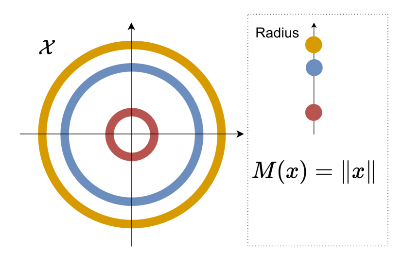
(a) Rotation

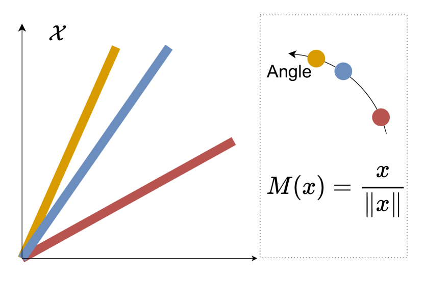
(b) Scaling

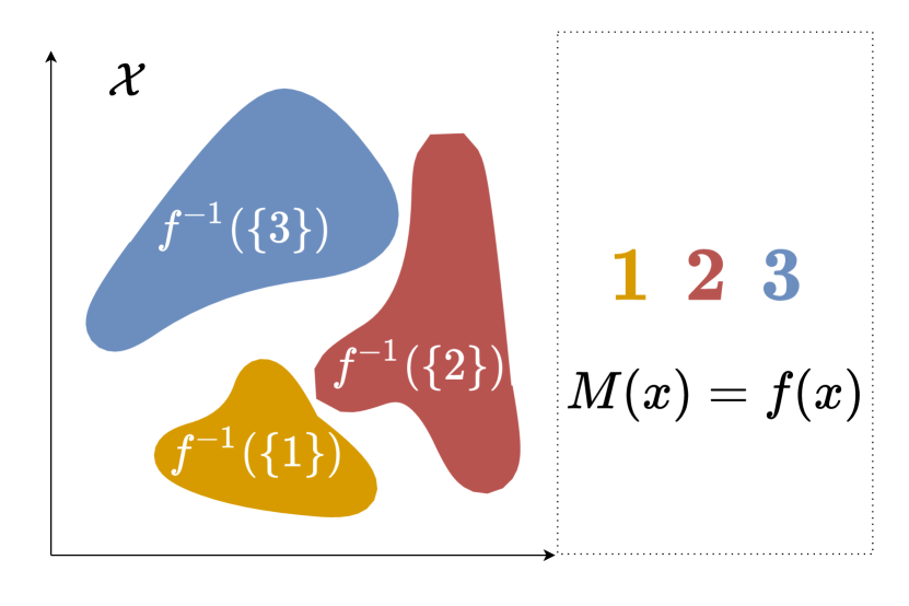
(c) Any transformation $f$

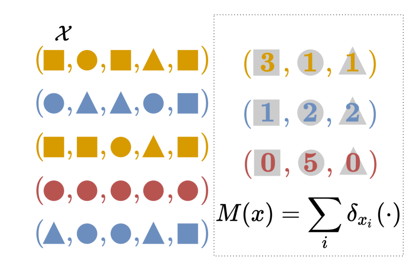
(d) Permutation

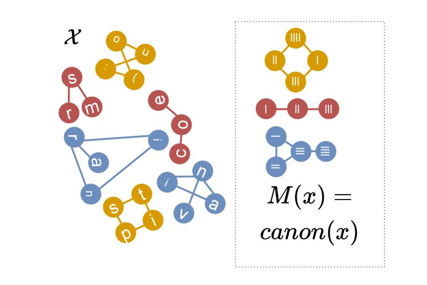
(e) Graph isomorphism

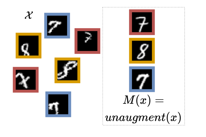
(f) Any data augmentation

Figure 1: Maximal invariants $M(X)$ are representatives of equivalence classes. Example $M$s include the: (a) Euclidean norm for rotations; (b) unit vector for scaling; (c) $f$ when equivalence classes are pre-images by $f$; (d) empirical measure for permutations; (e) canonical graph for graph isomorphisms; (f) unaugmented input for data augmentations.

We consider a general notion of invariance, namely invariance specified by an equivalence relation $\sim$ on $\mathcal{X}$. The equivalence induces a partition of $\mathcal{X}$ into disjoint equivalence classes, and we are interested in tasks whose conditional distributions are constant within these classes.

Definition 1.

The set of invariant tasks of interest with respect to an equivalence $(\mathcal{X},\sim)$, denoted $\mathcal{T}_{\scriptscriptstyle\sim}{}$, is all random variables $Y$ such that $x\sim x^{+}\implies p(Y\,|\,x)=p(Y\,|\,x^{+})$ for any $x,x^{+}\in\mathcal{X}$.

3.3 Rate-distortion theory for invariant task prediction

The key to simplifying $\mathrm{D}_{\scriptscriptstyle\mathcal{T}_{\scriptscriptstyle\sim}{}}$ is the existence of a (non-unique) worst-case invariant task, denoted $M(X)$. Such task contains all and only information to which tasks $Y\in\mathcal{T}_{\scriptscriptstyle\sim}$ are not invariant; we call them maximal invariants. A maximal invariant $M({\,\vbox{\hbox{\scalebox{0.75}{$\bullet$}}}\,})$ with respect to $\sim$ is any function satisfying

$$x\sim x^{+}\iff M(x)=M(x^{+})\quad\text{for any $x,x^{+}\in\mathcal{X}$.}$$ (3)

A maximal invariant removes all information that tasks are invariant to, as it maps equivalent inputs to the same output, i.e., $M(x)=M(x^{+})$. Yet, it retains the minimal information needed to perform invariant tasks, by mapping non-equivalent inputs $x\not\sim x^{-}$ to different outputs $M(x)\neq M(x^{-})$. In other words, $M(x)$ indexes the equivalence classes. For example, the Euclidean norm is a maximal invariant for rotation invariance, as all vectors that are rotated versions of one another can be characterized by their radial coordinate. For data augmentations, the canonical (unaugmented) version of the input is a maximal invariant. Other examples are shown in Fig. 1.

We prove in Sec. B.2 that under weak regularity conditions, maximal invariant tasks exist in $\mathcal{T}_{\scriptscriptstyle\sim}{}$, and that they achieve the supremum in Eq. 2. This allows us to show that $\mathrm{D}_{\scriptscriptstyle\mathcal{T}_{\scriptscriptstyle\sim}{}}$ reduces to the Bayes risk of predicting $M(X)$ from $Z$ and that it is a valid distortion measure. Crucially, this allows us to quantify downstream performance without enumerating invariant tasks.

Proposition 1.

Let $(\mathcal{X},\sim)$ be an equivalence relation and $M$ a maximal invariant that takes at most countably many values, with $\operatorname{H}\negthinspace\left[M(X)\right]<\infty$. Then $\mathrm{D}_{\scriptscriptstyle\mathcal{T}_{\scriptscriptstyle\sim}{}}$ (2) with log loss is a valid distortion and

$$\operatorname{D_{\scriptscriptstyle\mathcal{T}_{\scriptscriptstyle\sim}{}}}\negthinspace\left[X,Z\right]{}{}=\operatorname{R}\negthinspace\left[M(X)\,|\,Z\right]\;.$$ (4)

Here we used $\operatorname{R}\negthinspace\left[M(X)\,|\,X\right]=0$, as $M$ is a deterministic function. Also, note that the countable requirement holds when tasks are invariant to some rounding of the input, as is typically the case due to floating-point storage. We accommodate the uncountable case for squared-error loss in Sec. B.6.

With a valid distortion in hand, we invoke the RD theorem with $\mathrm{D}_{\scriptscriptstyle\mathcal{T}_{\scriptscriptstyle\sim}{}}$ to obtain our “Rate-Invariance” (RI) theorem. The RI theorem characterizes the bit-rate needed to store $X$ while ensuring small log-loss on invariant tasks. We obtain analogous results for squared-error loss.

Theorem 2 (Rate-Invariance).

Assume the conditions of Prop. 1. Let $\delta\geq 0$, and $Rate(\delta)$ denote the minimum achievable bit-rate for transmitting $Z$ such that for any $Y\in\mathcal{T}_{\scriptscriptstyle\sim}$ we have $\operatorname{R}\negthinspace\left[Y\,|\,Z\right]-\operatorname{R}\negthinspace\left[Y\,|\,X\right]\leq\delta$. Then $Rate(\delta)=0$ if $\delta\geq\operatorname{H}\negthinspace\left[M(X)\right]$ and otherwise it is finite and

$$Rate(\delta)\quad=\quad\underbrace{\ \vphantom{\sum}\operatorname{H}\negthinspace\left[M(X)\right]}_{\begin{subarray}{c}\text{information needed}\\ \text{to predict }\mathcal{T}_{\scriptscriptstyle\sim}{}\end{subarray}}\quad\underbrace{-\ \vphantom{\sum}\delta}_{\begin{subarray}{c}\text{acceptable decrease}\\ \text{in predictive loss}\end{subarray}}\quad=\quad\underbrace{\vphantom{\sum}\operatorname{H}\negthinspace\left[X\right]}_{\begin{subarray}{c}\text{standard}\\ \text{compression}\end{subarray}}\quad\underbrace{-\ \vphantom{\sum}\operatorname{H}\negthinspace\left[X\,|\,M(X)\right]}_{\begin{subarray}{c}\text{gains due to}\\ \text{invarainces}\end{subarray}}\quad-\ \delta.$$ (5)

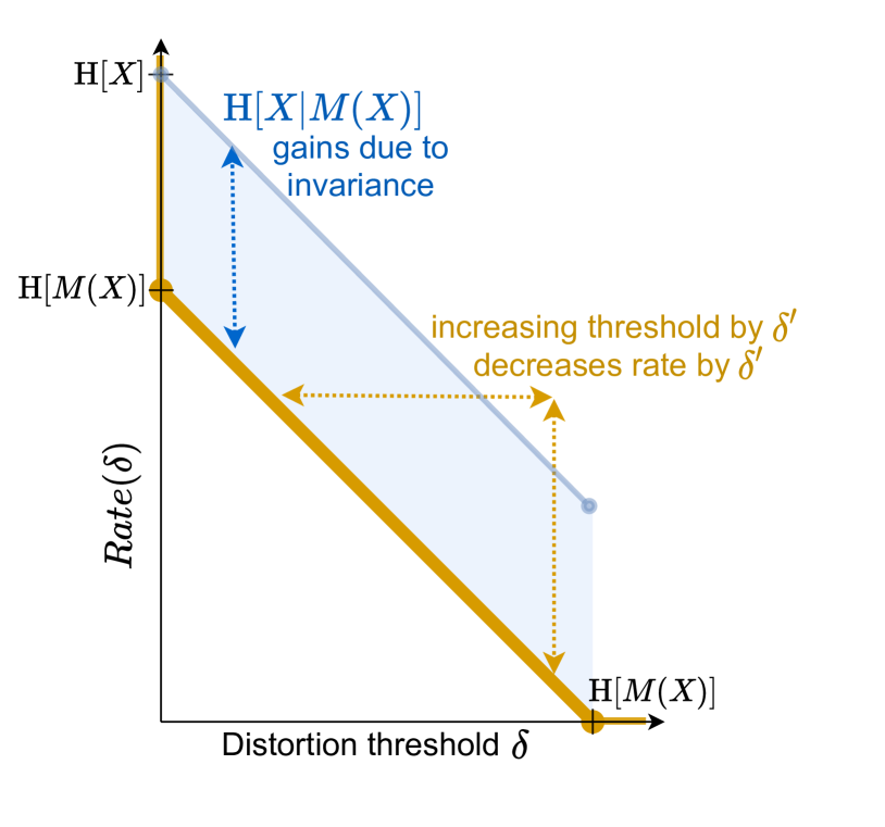
Figure 2: Rate-Invariance function.

To ensure lossless prediction, i.e., $Rate(0)$, our theorem states that we require a bit-rate of $\operatorname{H}\negthinspace\left[M(X)\right]$. Intuitively, this is because $M(X)$ contains the minimal information needed to predict losslessly any $Y\in\mathcal{T}_{\scriptscriptstyle\sim}{}$. Furthermore, the theorem relates compression and prediction by showing that allowing a $\delta$ decrease in log-loss performance on all tasks can save exactly $\delta$ bits. Intuitively, this is a linear relationship, because expected log-loss is measured in bits. On the right of Eq. 5 we further decompose $\operatorname{H}\negthinspace\left[M(X)\right]$ into two terms to provide another interpretation: (i) $\operatorname{H}\negthinspace\left[X\right]$, which, for discrete $X$, is the bit-rate required to losslessly compress $X$, and (ii) $\operatorname{H}\negthinspace\left[X\,|\,M(X)\right]$, which quantifies the information removed due to the invariance of desired tasks. Importantly, removing this information does not impact the best possible predictive performance. See Fig. 2.

The bit-rate gains can be substantial, depending on the invariances. Consider compressing a sequence of $n$ i.i.d. fair coin flips. Suppose one is only interested in predicting permutation invariant labels. Then instead of compressing the entire sequence in $\operatorname{H}\negthinspace\left[X^{n}\right]=n\operatorname{H}\negthinspace\left[X\right]=n$ bits, one could compress the number of heads, which is a maximal invariant for permutation invariance, in $\mathcal{O}(\log n)$ bits. As more interesting examples, we recover in Sec. B.4 results from 1 unlabeled graph compression [20]; 2 multiset compression [21]; 3 single task compression (IB; [11]). The equivalence $\sim$ can be induced by any transformations, such as transforming an image to its caption. We use this idea in Sec. 5.3 to obtain >$1000\times$ compression on ImageNet without sacrificing predictive performance.

4 Unsupervised training of invariant neural compressors

In this section, we design practical, invariant neural compressors that bound optimal rates. Derivations are in Appx. C. In particular, we are interested in the $\operatorname*{arg\,min}$ encoders $p(Z|X)$ of the RD function (Eq. 1) under the invariance distortion $\mathrm{D}_{\scriptscriptstyle\mathcal{T}_{\scriptscriptstyle\sim}{}}$. To accomplish this, we can optimize the following equivalent (i.e., it induces the same RI function) Lagrangian, where $\beta$ takes the role of $\delta$,

$$\operatorname*{arg\,min}_{p(Z|X)}\quad\operatorname{I}\negthinspace\left[X;Z\right]\;+\;\beta\cdot\operatorname{R}\negthinspace\left[M(X)\,|\,Z\right].$$ (6)

In ML, the maximal invariant $M$ is often not available. Instead, invariances are implicitly specified by sampling a random augmentation from $A$, applying it to a datapoint $X$, and asking that the model’s prediction be invariant between $X$ and $A(X)$. For example, invariance to cropping can be enforced by randomly cropping images while retaining the original label. We show in Appx. C, that in such case, we can treat the augmented $A(X)$ as the new source, $Z$ as the representation of $A(X)$, and the unaugmented $X$ as the maximal invariant task $M(A(X))$. Indeed, $\operatorname{R}\negthinspace\left[M(A(X))\,|\,Z\right]$ is equal to $\operatorname{R}\negthinspace\left[X\,|\,Z\right]$ up to a constant, so we can rewrite Eq. 6 as the following equivalent objective,

$$\operatorname*{arg\,min}_{p(Z|A(X))}\quad\operatorname{I}\negthinspace\left[A(X);Z\right]\;+\;\beta\cdot\operatorname{R}\negthinspace\left[X\,|\,Z\right].$$ (7)

Such reformulation is possible if random augmentations retain the invariance structure $X\sim A(X)$ but “erase” enough information about equivalent inputs, specifically, if $X{\perp\!\!\!\perp}A(X)\,|\,M(X)$. We discuss the second requirement in Appx. C but note that it will likely not be a practical issue if the dataset is small compared to the support $|\mathcal{D}|\ll|\mathcal{X}|$. With this, we have an objective whose r.v.s. are easy to sample from. However, both terms in Eq. 7 are still challenging to estimate.

In the following, we develop two practical variational bounds to Eq. 7, which can be optimized by stochastic gradient descent [23] over the encoder’s parameters. Both approximations use the standard lossy neural compression bound $\operatorname{I}\negthinspace\left[Z;A(X)\right]\leq\operatorname{H}\negthinspace\left[Z\right]\leq\min_{\theta}\operatorname{E}_{p(Z)}\negthinspace\left[-\log q_{\theta}(Z)\right]$ where $q_{\theta}(Z)$ is called an entropy model (or a prior) [24, 25]. This has the advantage that the learned $q_{\theta}$ can be used for entropy coding $Z$ [26, 27]. See Ballé et al. [28] for possible entropy models. Our two approximations differ in how they upper bound $\operatorname{R}\negthinspace\left[X\,|\,Z\right]$. The first uses a reconstruction loss, which attempts to reconstruct the unaugmented input $x\in\mathcal{D}$ from $A(x)$. The second uses a discrimination loss, which attempts to recognize which examples are augmented versions of the input.

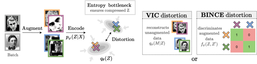
Figure 3: Our unsupervised objectives for invariant image compression under data augmentation use the same encoder, but differ in their approximation to the invariance distortion. Both models encode the augmented data, pass the representation through an entropy bottleneck which ensures that they are compressed, and use a distortion to retain the information about the identity of the original data. The models differ in how they retain that information: (VIC) by reconstructing unaugmented inputs; (BINCE) by recognizing which inputs come from the same original data.

4.1 Variational Invariant Compressor (VIC)

Our first model is a modified neural compressor in which inputs are augmented but target reconstructions are not. We refer to it as a variational invariant compressor (VIC). See Fig. 3 for an illustration. VIC has an encoder $p_{\varphi}(Z|A(X))$, an entropy model $q_{\theta}(Z)$, and a decoder $q_{\phi}(X|Z)$. Given a data sample $x\in\mathcal{D}$, we apply a random augmentation $A(x)$, and encode it to get a representation $Z$. The decoder then attempts to reconstruct the unaugmented $x$ from $Z$. This leads to the objective,

$$\mathcal{L}_{\scriptscriptstyle\text{VIC}}{}(\phi,\theta,\varphi)\vcentcolon=-\sum_{x\in\mathcal{D}}\operatorname{E}_{p(A)p_{\varphi}(Z|A(x))}\negthinspace\left[\log q_{\theta}(Z)+\beta\cdot\log q_{\phi}(x\,|\,Z)\right].$$ (8)

The term $\log q_{\theta}(Z)$ is an entropy bottleneck, which bounds the rate $\operatorname{I}\negthinspace\left[A(X);Z\right]$ and ensures that unnecessary information is removed. The term $\log q_{\phi}(x\,|\,Z)$ bounds the distortion $\operatorname{R}\negthinspace\left[X\,|\,Z\right]\leq\operatorname{E}_{p(X,Z)}\negthinspace\left[-\log q_{\phi}(X\,|\,Z)\right]$ and ensures that VIC preserves the information needed for invariant tasks.

4.2 Bottleneck InfoNCE (BINCE)

Our second compressor retains all predictive information without reconstructing the data. It has two components: an entropy bottleneck and an InfoNCE [15] objective, which is the standard in contrastive SSL. We refer to this as the bottleneck InfoNCE (BINCE), see Fig. 3. BINCE has an advantage over VIC in that it avoids the problem of reconstructing possibly high dimensional data.

Algorithm 1 BINCE’s forward pass for $x$

1:$p_{\varphi}$, $q_{\theta}$, $f_{\psi}$, $\mathcal{D}$, $A$, $\beta$, $n$, $x$

2:$\tilde{x}\leftarrow\text{sample}(A(x))$ $\triangleright$ Augment

3:$z\leftarrow\mathrm{sample}(p_{\varphi}(Z|\tilde{x}))$ $\triangleright$ Encode

4:$\mathrm{rate\_loss}\leftarrow-\log q_{\theta}(z)$

5:$\{x_{i}^{-}\}_{i=1}^{n}\leftarrow\mathrm{select}(\mathcal{D}\setminus\negthinspace\left\{x\right\})$ $n$ times

6:$\tilde{\mathbf{x}}\leftarrow\text{sample}([A(x),A(x_{1}^{-}),\dots,A(x_{n}^{-})])$

7:$\mathbf{z}\leftarrow\mathrm{sample}(p_{\varphi}(Z|\tilde{\mathbf{x}}))$

8:$z^{+}\leftarrow\mathbf{z}[0]$

9:$\mathrm{softmax}\leftarrow\frac{\exp f_{\psi}(z^{+},z)}{(\sum_{z^{\prime}\in\mathbf{z}}\exp f_{\psi}(z^{\prime},z))}$

10:$\mathrm{distortion\_loss}\leftarrow-\log(\mathrm{softmax})$

11:return $\mathrm{rate\_loss}+\beta\cdot\mathrm{distortion\_loss}$

Algorithm 1 shows how to train BINCE, where each call to $A$ returns an independent augmentation of its input. As with VIC, for every datapoint $x\in\mathcal{D}$, we obtain a representation $Z$ by applying an augmentation $A(x)$ and passing it through the encoder $p_{\varphi}(Z\,|\,A(X))$. We then sample a “positive” example $Z^{+}$ by encoding a different augmented version of the same underlying datapoint $x$. Finally, we sample $n$ “negative” examples $Z_{i}^{-}$ by encoding augmentations $A(x_{i}^{-})$ of datapoints $x_{i}^{-}\in\mathcal{D}$ that are different from $x$. This results in a sequence $\bm{Z}=(Z^{+},Z_{1}^{-},\ldots,Z_{n}^{-})$. For conciseness we will denote the above sampling procedure as $p_{\varphi}(Z,\bm{Z}\,|\,A,\mathcal{D},x)$. The final loss uses a discriminator $f_{\psi}$ that is optimized to score the equivalence of two representation,

$$\mathcal{L}_{\scriptscriptstyle\text{BINCE}}{}(\varphi,\theta,\psi)\vcentcolon=-\sum_{x\in\mathcal{D}}\operatorname{E}_{p(A)p_{\varphi}(Z,\bm{Z}|A,\mathcal{D},x)}\negthinspace\left[\log q_{\theta}(Z)+\beta\cdot\log\frac{\exp f_{\psi}(Z^{+},Z)}{\sum_{Z^{\prime}\in\mathbf{Z}}\exp f_{\psi}(Z^{\prime},Z)}\right].$$ (9)

BINCE retains the necessary information by classifying (as seen by the softmax) which $Z$ is associated with an equivalent example $X$. Both VIC and BINCE give rise to efficient compressors by passing $X$ through $p_{\varphi}(Z|X)$ and entropy coding using $q_{\theta}(Z)$. In theory they can both recover the optimal rate for lossless predictions, i.e., $\operatorname{H}\negthinspace\left[M(X)\right]$, in the limit of infinite samples ($|\mathcal{D}|$,$n$) and unconstrained variational families. In practice, BINCE has the advantage over VIC of 1 not requiring a high dimensional decoder; and 2 giving (for suitable $f_{\psi}$) representations that are approximately linearly separable [29, 30, 31] and thus easy to predict from [32, 15]. The disadvantages of BINCE are that it 1 does not provide to reconstructions diminishes interpretability; and 2 has a high bias, unless the number of negative samples $n$ is large [33, 34], which is computationally intensive.

5 Experiments

We evaluated our framework focusing on two questions: 1 What compression rates can our framework achieve at what cost? 2 Can we train a general purpose predictive image compressor? For all experiments, we train the compressors, freeze them, train the downstream predictors, and finally evaluate both on a test set. For classical compressors, standard neural compressors (VC) and our VIC, we used either reconstructions $\tilde{X}$ as inputs to the predictors or representations $Z$. As BINCE does not provide reconstructions, we predicted from the compressed $Z$ using a multi-layer perceptron (MLP). We used ResNet18 [35] for encoders and image predictors. For entropy models we used Ballé et al.’s [28] hyperprior, which uses uniform quantization. We optimized hyper-parameters on validation using random search. For classification tasks, we report classification error instead of log-loss. The former is more standard and gave similar results (see Sec. F.2). For experimental details see Appx. E. For additional results see Appx. F. Code is at github.com/YannDubs/lossyless.

5.1 Building intuition with toy experiments

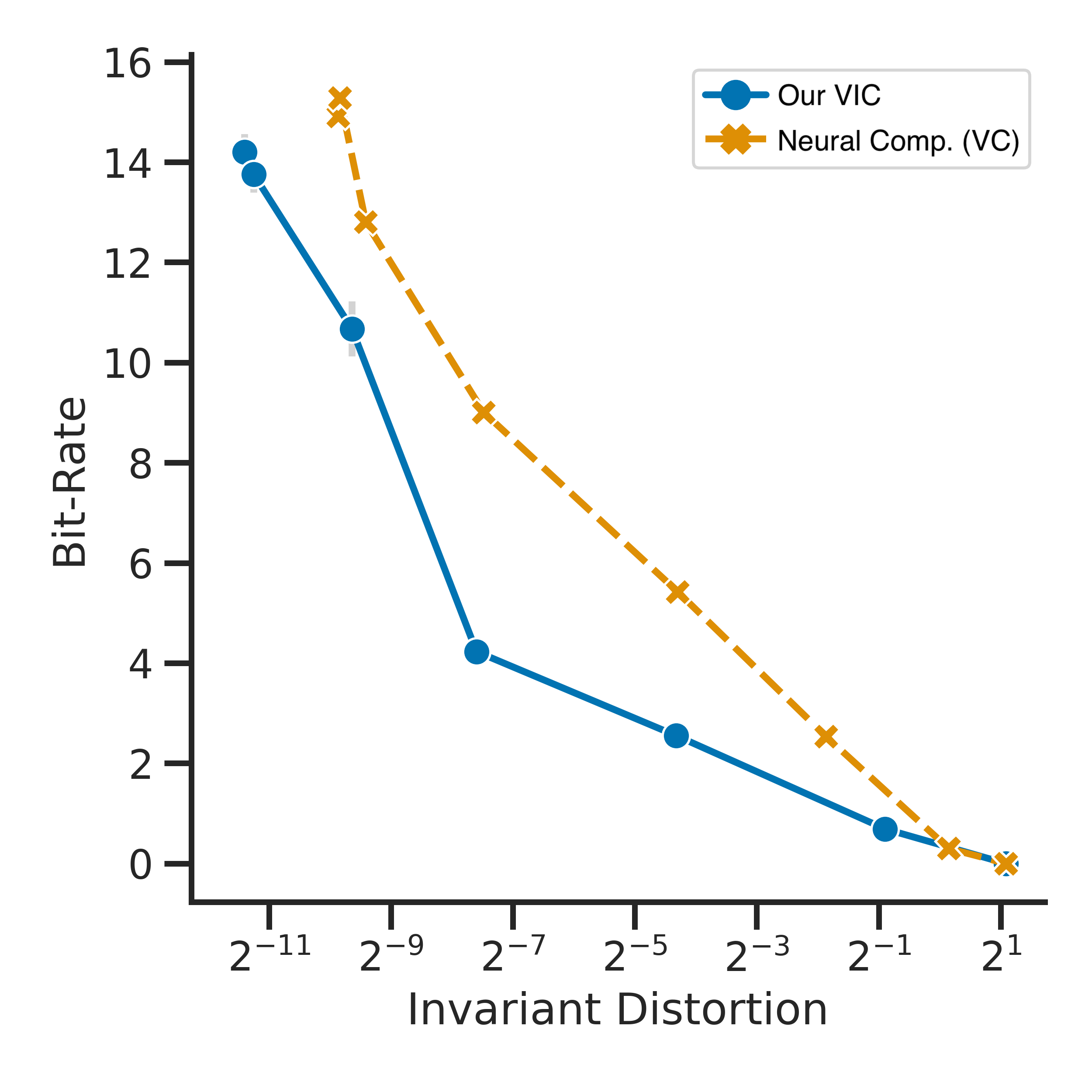
(a) Rate-Invariance curves

(b) VC high rate

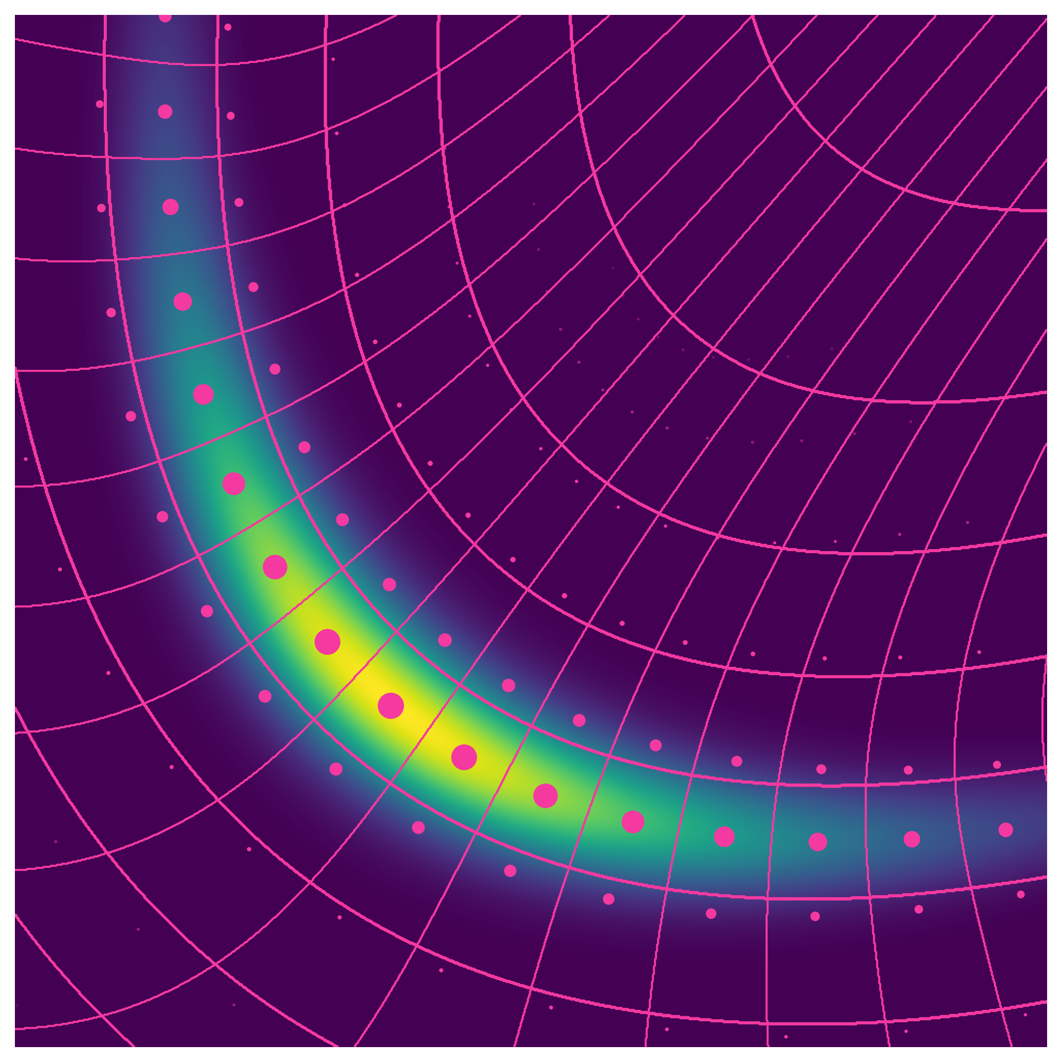
(c) VC

(d) VC low rate

(e) VIC high rate

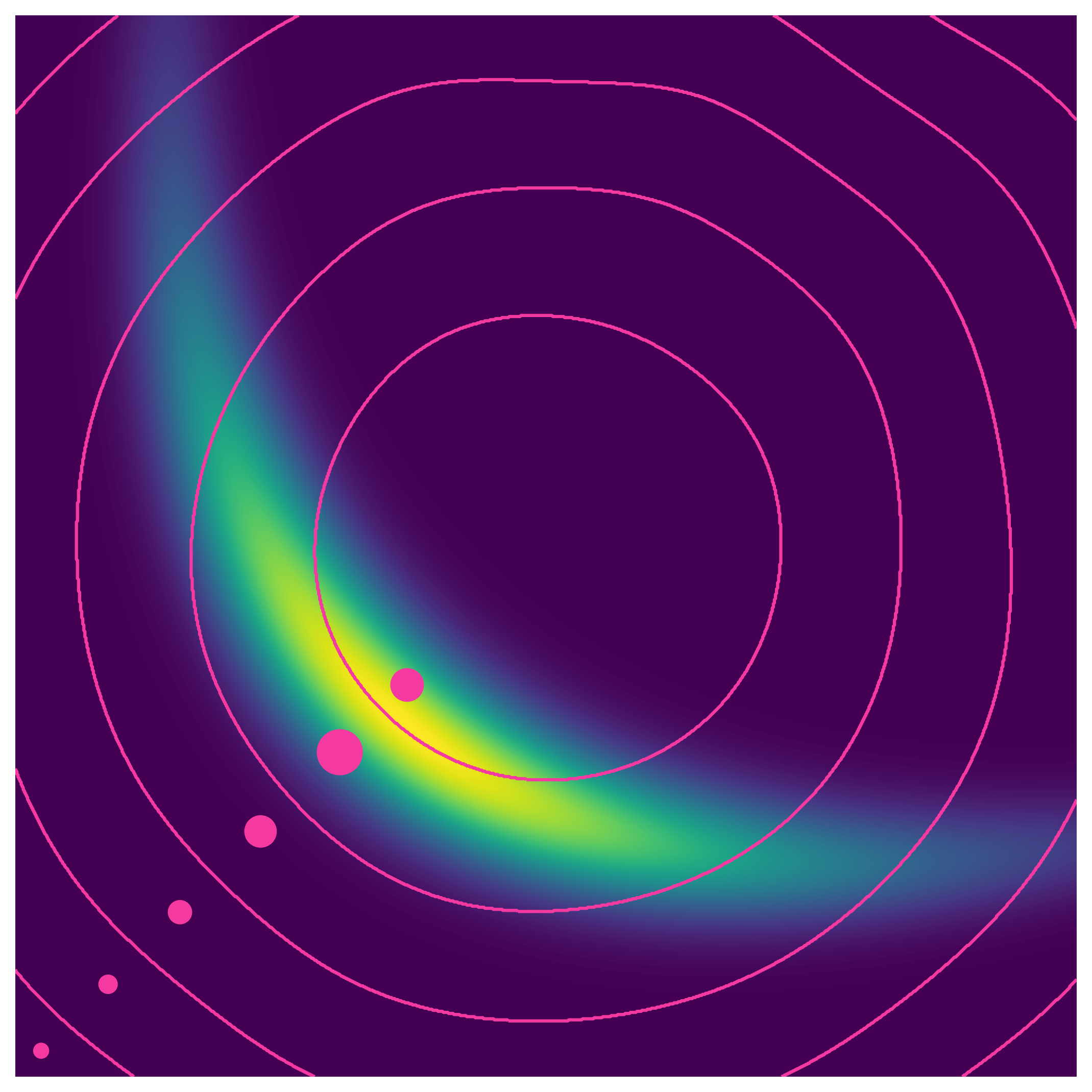
(f) VIC

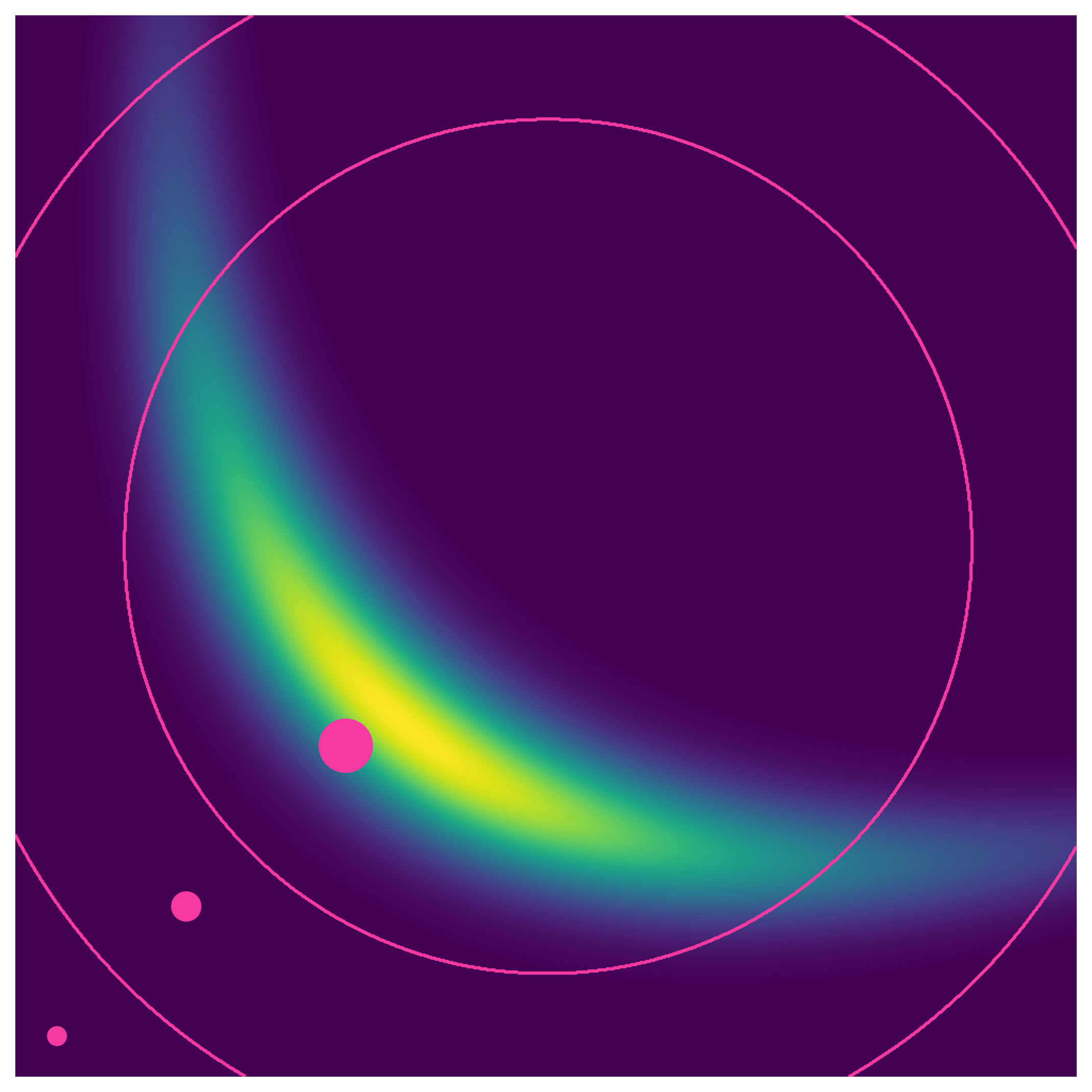
(g) VIC low rate

Figure 4: Compression rates of a Banana source [36] can be decreased when downstream tasks are rotation invariant. (Left) Our invariant compressor (VIC, blue) outperforms neural compressors (VC, orange). 5 runs with standard errors in gray. (Right) VIC quantizes the space using disks to remove unnecessary angular information. Pink lines are quantization boundaries, dots are code vectors with size proportional to learned probabilities. Low rates correspond to low $\beta$ in Eq. 7.

To build an visual intuition, we compressed samples from a 2D banana source distribution [36], assuming rotation invariant tasks, e.g., classifying whether points are in the unit circle. We also compressed MNIST digits as in Fig. 1. Digits are augmented (rotations, translations, shearing, scaling) both at train and test time to ensure that our invariance assumption still holds.

Where do our rate gains come from? For rotation invariant tasks, our method (VIC) discards unnecessary angular information by learning disk-shaped quantizations (Fig. 4, bottom right). Specifically, VIC retains only radial information by mapping all randomly rotated points (disks) back to maximal invariants (pink dots). In contrast, standard neural compressors (VC) attempt to reconstruct all information, which requires a finer partition (Fig. 4, top right). As a result (Fig. 4(a)), VIC needs a smaller bit-rate ($y$-axis) for the same desired performance ($\mathrm{D}_{\scriptscriptstyle\mathcal{T}_{\scriptscriptstyle\sim}{}}$, $x$-axis). The area under the RD curve (AURD) for VIC is $35.8{\scriptsize\pm 4.2}$ against $48.1{\scriptsize\pm 0.3}$ for VC, i.e., expected bit-rate gains are around $70\%$. Similar gains are achieved for augmented MNIST in Fig. 5 by reconstructing canonical digits.

(a) Rate-Error curve

(b) Reconstructions that allow $99\%$ downstream accuracy

Figure 5: (Left) By reconstructing prototypical digits our VIC (blue) achieves higher compression of augmented MNIST digits than standard neural compressors (VC, orange) without hindering downstream classification. 5 runs. (Right) The source examples (first row) as well as reconstructions for the non-invariant (second row) and invariant compressor (last row).

Can we recover the optimal bit-rate? We investigated whether our losses can achieve the optimal bit-rate for lossy prediction by using supervised augmentations, i.e., $A(x)$ randomly samples a train example $x^{+}$ that has the same label. For MNIST the single-task optimal bit-rate is $\operatorname{H}\negthinspace\left[Y\right]=\log(10)\approx 3.3$ bits. VIC and BINCE respectively achieve $5.7$ and $5.9$ bits, which shows that our losses are relatively good despite practical approximations. Details in Sec. F.2.

What is the impact of the choice of augmentations? The choice of augmentation $A$ implicitly defines the desired task-set $\mathcal{T}{}$, i.e., $\mathcal{T}{}$ is the set of all tasks for which $A$ does not remove information. As a result Theorem 2 can be rewritten as $Rate(\delta)=\operatorname{I}\negthinspace\left[X;A(X)\right]-\delta$, so the rate decreases when $A$ removes more information from $X$. To illustrate this we trained our VIC using three augmentation sets on MNIST, all of which keep the true label invariant but progressively discard more $X$ information. VIC respectively achieves a rate of $185.3$, $79.0$, and $5.7$ bits, which shows the importance of using augmentations that remove $X$ information. Details and BINCE results are in Sec. F.2.

5.2 Evaluating our methods with controlled experiments

To investigate our methods, we compressed the STL10 dataset [37]. We augment (flipping, color jittering, cropping) the train and test set, to ensure that the task invariance assumptions are satisfied. We focus on more realistic settings in the next section. In each experiment, we sampled $100$ combinations of hyper-parameters to ensure equal computational budget across models and baselines.

Table 1: Invariant compressors (BINCE, VIC) outperform classical (PNG, JPEG, WebP) and neural (VC) compressors on STL10. BINCE achieves lossless prediction but compresses $121\times$ better.

	PNG [38]	JPEG [39]	WebP [40]	VC $\tilde{X}$	VIC $\tilde{X}$	VIC $Z$	BINCE
Decrease in test acc.	$0$	$0.7$	$1.1$	$21.0$	$25.1$	$16.1$	$0.0$
Compression gains	$1\times$	$3\times$	$13\times$	$63\times$	$269\times$	$175\times$	$121\times$

How do our BINCE and VIC compare to standard compressors? In Table 1 we compare compressors at the lowest downstream error that they achieved. As benchmark, we use PNG’s lossless compression. Predicting from PNG corresponds to standard image classification, and obtains a rate of $1.42\text{e}4$ bits per image for $80.8\%$ accuracy. Classical lossy methods (JPEG, WebP) achieved up to $13\times$ bit-rate gains with little drop in performance. In comparison, our BINCE method achieved $121\times$ compression gains with no impact on predictions. Both our invariant (VIC) and standard (VC) neural compressors significantly decreased classification accuracy, which we believe can be explained by the encoders architecture (ResNet18) that we use for consistency (see Sec. F.3).

Should we predict from representations $Z$ or reconstructions $X$? In Table 1 we analyzed the impact of predicting from $Z$ instead of $\tilde{X}$ for VIC and see that this increases accuracy by $9\%$. In contrast, predicting from $Z$ for VC decreases performance by $12\%$ (see Sec. F.3). This suggests that invariant reconstructions $\tilde{X}$ might not be easy to predict from with standard image predictors.

Are we learning invariant compressors? Invariant compressors should provide RD curves that are robust to test distribution shift in the desired augmentations. We thus trained our VIC by applying the augmentations $50\%$ of the time but varying that probability $p$ at test time. In Sec. F.3 we show that this distribution shift have negligible influence on RD curves.

5.3 A zero-shot compressor using pre-trained self-supervised models

BINCE includes a standard contrastive SSL loss. So, we investigated whether existing pre-trained SSL models [32, 41] can be used to build generic compressors. In particular, we investigated whether CLIP [41] could be quickly turned into a powerful task-centric compressor for computer vision. In the introduction, we motivated large compression gains by noting that typical image classification tasks can be predicted from detailed captions instead of images (around $1000\times$ more bits). CLIP is a vision transformer [42] pre-trained on 400M pairs of images and text $(x_{image},x^{+}_{text})$ using a contrastive loss. The “augmentation” $A$ is then a function that maps $x_{image}$ to its associated $x^{+}_{text}$ and vis-versa. This will partition the images and texts into sets, each of which are associated directly or by transitivity in CLIP’s dataset. This suggests that CLIP is retaining the image information that corresponds to a detailed caption, and may be turned into a generic compressor for image classification.

CLIP can essentially be seen as a BINCE model with an image-to-text augmentation, but without an entropy bottleneck. (For details about the CLIP-BINCE relation see Sec. C.5.) We thus constructed an approximation of our desired image-to-text BINCE compressor by two simple steps. First, we downloaded and froze CLIP’s parameters. Second, we trained, on the small MSCOCO dataset [43], an entropy bottleneck to compress CLIP’s representation. The latter step can be done by training any lossy compressor on CLIP’s representations, we did so using Ballé et al.’s [28] hyperprior entropy model with a learned rounded precision. We then evaluated our resulting compressor on 8 datasets (various classification tasks and image shapes) that were never seen during training (zero-shot), by training an MLP for downstream predictions on each dataset. One can see this as a multi-task setting (each dataset is a distinct task). We investigate the case of multiple labels per images in Sec. F.5.

Table 2: Converting a pretrained SSL model into a zero-shot compressor achieves substantial bit-rate gains while allowing test accuracies similar to supervised models predicting from raw images.

	ImageNet	STL	PCam	Cars	CIFAR10	Food	Pets	Caltech
Rate gains vs JPEG	$1104\times$	$35\times$	$64\times$	$131\times$	$7\times$	$109\times$	$150\times$	$126\times$
Our Acc. $[\%]$	$76.3$	$98.7$	$80.9$	$79.6$	$95.2$	$88.3$	$89.5$	$93.4$
Supervised Acc. $[\%]$	$76.1$	$99.0$	$82.6$	$49.1$	$96.7$	$81.8$	$90.4$	$94.5$

Can we use pretrained SSL to obtain a generic compressor? Table 2 shows that we can exploit existing state-of-the-art (SOTA) SSL models to get a powerful image compressor, which achieves $1000\times$ bit-rate gains on ImageNet compared to JPEG (at the quality level used for storing ImageNet). The bit-rate gains (1^st row) are significant across all zero-shot datasets, even for biological tissues (PCam; [44]). Importantly, these gains come at little cost in test performance. Indeed, the test accuracies of MLPs from our representations (2^nd row) is similar to a near SOTA model trained on the uncompressed images (3^rd row is from Radford et al. [41]). These results are not surprising as JPEG is optimized to retain perceptual rather than classification information. Note that the large variance in rate gains come from JPEG rates due to different images shapes (see Table 3).

Our CLIP compressor retains all the information needed to get 0 error for those tasks

Table 2 provides the test performance for MLPs, while our theory discusses Bayes risk, which is independent of specific predictors and generalization. We estimated the excess Bayes risk for our datasets by counting the images (in train and test) that get compressed to the same $Z$ but have different labels. We found that we are in the lossless prediction regime for those datasets.

Table 3: Our entropy bottleneck (EB) on CLIP improves compression of representations up to $17\times$ with little impact on predictions. The same compressor is used across datasets. Rates are per image.

		ImageNet	STL	PCam	Cars	CIFAR10	Food	Pets	Caltech
Bit-Rate	JPEG	1.49e6	4.71e4	9.60e4	1.92e5	1.05e4	1.54e5	1.81e5	1.69e5
	CLIP	1.52e4	1.52e4	1.52e4	1.52e4	1.52e4	1.52e4	1.52e4	1.52e4
	+EB high $\beta$	2.47e3	2.46e3	2.61e3	2.59e3	2.53e3	2.39e3	2.33e3	2.46e3
	+EB $\beta$	1.35e3	1.34e3	1.49e3	1.47e3	1.41e3	1.27e3	1.21e3	1.34e3
	+EB low $\beta$	9.63e2	9.52e2	1.09e3	1.07e3	1.02e3	8.89e2	8.35e2	9.53e2
Test Acc.	CLIP	76.5	98.6	84.5	80.8	95.3	88.5	89.7	93.2
	+EB high $\beta$	76.6	98.7	82.7	80.4	95.3	88.5	89.6	93.5
	+EB $\beta$	76.3	98.7	80.9	79.6	95.2	88.3	89.5	93.4
	+EB low $\beta$	76.0	98.7	80.1	78.9	94.8	87.6	88.6	92.9

What is the effect of the entropy bottleneck? In Table 3 we compare the pretrained CLIP, to our CLIP compressor with an entropy bottleneck (EB) trained at different values for $\beta$. When trained with a high $\beta$, our EB improves bit-rates by an average of $6\times$ without impacting predictions. For our compressor from Table 2 (CLIP+EB $\beta$) the gains increase to $11\times$ with little predictive impact. The sacrifice in predictions is more clear for $16\times$ bit-rate gains (low $\beta$). This shows that CLIP’s raw representations retain unnecessary information as it not explicitly trained to discard information.

How would end-to-end BINCE compare to staggered training? Compression gains can likely be larger by end-to-end training of BINCE, which would require access to CLIP’s original dataset. To get an idea of potential gains we compared end-to-end and staggered BINCE on augmented MNIST in Sec. F.2. We found significant rate improvements ($358$ to $131$ bits) for similar test accuracy.

Our CLIP compressor is simple to use

In Sec. E.7, we provide a minimal script (150 lines) to train a generic compressor in less than five minutes on a single GPU. The script contains an efficient entropy coder for our model (200 images/second), which shows its practicality. As usual in SSL, the compressed representations are also more computationally efficient to work with than standard compressors. In our minimal script we achieve the desired performance ($98.7\%$ on STL) using a linear model that is trained in one second, which is $1000\times$ faster than the baseline in Table 2. This shows that our pipeline can improve computational efficiency in addition to storage efficiency.

Table 4: Text-image invariance is better than invariance to standard augmentations for image classification. CLIP and SimCLR are both ResNet50 pretrained with InfoNCE but different augmentations.

		ImageNet	STL	PCam	Cars	CIFAR10	Food	Pets	Caltech
Rate	CLIP+EB	$2108$	$1962$	$1949$	$2421$	$2111$	$1991$	$1867$	$1968$
	SimCLR+EB	$2811$	$2732$	$2769$	$2751$	$2950$	$2077$	$2839$	$2502$
Acc.	CLIP+EB	$63.2$	$92.0$	$78.6$	$68.0$	$65.5$	$74.1$	$81.8$	$83.0$
	SimCLR+EB	$62.8$	$91.9$	$81.4$	$29.6$	$78.6$	$60.0$	$78.9$	$79.0$

What augmentations to use for SSL compression? Table 4 compares two ResNet50 pretrained with contrastive learning using invariance to text-image (CLIP) or standard image augmentations (SimCLR [32]) such as cropping or flipping. We see that CLIP’s augmentation usually give better compression and downstream performance, which shows the importance of the choice of augmentations. This also supports our motivation of using text-image augmentations, which are likely label-preserving for a vast amount of tasks but discard large amounts of unnecessary information.

6 Related work

In Appx. D we discuss more related work, including invariances in compression and the link to SSL.

Task-centric compression

To our knowledge, our paper is the first to formalize compression only for predictions. IB [11] uses a task-centric distortion, but is not used for compression as it requires supervised training, so there are no advantages compared to compressing predicted labels. Some authors used heuristics to bypass the supervised issue, e.g., focusing on low frequencies for classification [45] or high frequencies for segmentation [46]. Other authors have incorporated predictive errors to perceptual distortions [47, 48], but cannot compress without the perceptual distortion for the same reason as IB. One exception is Weber et al.’s [49] compressor, which (when removing their perceptual distortion) minimizes MSE in the hidden layers of a pretrained classifier. Even more related is Singh et al.’s [50] work on compressing pretrained features for transfer learning, which is practice is similar to our compression of SSL features. Their work do not provide theoretical justifications, and are constrained to tasks that are similar to those used for pretraining.

7 Discussion and Outlook

Given the ever increasing amount of data that is processed by task-specific algorithms, it is necessary to rethink the current task-agnostic compression paradigm. We formalized the first compression framework for retaining only the information necessary for high performance on desired tasks. Using our theory, we provide two unsupervised objectives for training neural compressors. Experimentally, we show that these compressors can achieve bit-rates that are orders of magnitude ($1000\times$ on ImageNet) smaller than standard image compressors without losing predictive performance.

There are a number of caveats that should be addressed. First, to achieve better rates, our theory requires an irrecoverable loss of information. This can be an issue if the set of desired tasks changes. For example, if one uses text-image invariances then it may be impossible to perform image segmentation from the compressed representations. One solution would be to keep an original copy and use invariant compression for duplicated data, e.g., for the thousands copies of ImageNet. A second issue is the interpretability of the compressed representations. This can be partially addressed by reconstructing prototypical data as in Fig. 1 (post-hoc decoders could be trained for BINCE). A third caveat is that the compressed representations may be harder to learn from, e.g., neural networks may struggle to predict from representations even if the information is retained. Although our experiments actually showed the opposite, this should be addressed theoretically, e.g., using decodable information [51, 52]. Finally, successful use of our framework requires access to label-preserving augmentations $A$ that discard significant information about $X$. Finding such an $A$ may be challenging for some tasks. Given that augmentations are ubiquitous in ML, the community will hopefully continue developing task-specific augmentations which we could take advantage of.

Nevertheless, we achieved orders of magnitude improvements in compression for predictions, and we believe that our improvements are just the beginning. For example, many tasks can be answered by referencing a detailed natural language description of the data. In these cases, the improvements can be very large, potentially 1M$\times$ for videos. In the long-term, we hope that abandoning perceptual reconstructions will enable individuals to process data at scales that are currently only possible at large institutions, and our society to take advantage of large data sources in a more sustainable way.

Appendix

Appendix A Preliminaries

A.1 Notation

Probability  We assume a background standard probability space $(\Omega,\mathcal{H},\mathbb{P})$ that is rich enough to support all random variables used. Letters that are upper-case $X$ represent a random variable, while realizations are denoted with the associated lower case $x$. The sample space of a random variable will be written using a calligraphic $\mathcal{X}$, and we will say that $X$ takes value in (t.v.i) $\mathcal{X}$. We denote the probability distribution of $X$ as $P(X)$ and the probability density function, if it exists, as $p(X)$. $X\overset{\raisebox{-2.0pt}{\smash{\text{\tiny d}}}}{\sim}\mathcal{N}(0,1)$ denotes that $X$ has a certain distribution (here, Gaussian). Expectations are written as: $\operatorname{E}_{P(X)}\negthinspace\left[X\right]$, or $\operatorname{E}_{p(X)}\negthinspace\left[X\right]$ when the density exists. Independence between two random variables $X$ and $Y$ is denoted with $X{\perp\!\!\!\perp}Y$. To denote conditional independence between two random variables $X$ and $Y$ given $Z$ we either use $X{\perp\!\!\!\perp}Y\,|\,Z$ or say that $X-Z-Y$ forms a Markov Chain. $f\circ g$ denotes a composition of two functions $f$ and $g$, but in the case of random variable we also use the shorthand $f(X)\vcentcolon=f\circ X$.

Information theory  For notational convenience (see Assumption 5 below), when dealing with log loss we will always assume the existence of probability densities, in which case the KL divergence between two probability distributions on $\mathcal{X}$, $P$ and $Q$, is $\operatorname{D}_{\text{KL}}\negthinspace\left[p(X)\middle\|q(X)\right]\vcentcolon=\int p(X)\log\frac{p(X)}{q(X)}\,\mathrm{d}x$. The mutual information between random variables $X$ and $Z$ is $\operatorname{I}\negthinspace\left[X;Z\right]\vcentcolon=\operatorname{D}_{\text{KL}}\negthinspace\left[p(X,Z)\middle\|p(X)p(Z)\right]$. The (differential or discrete) entropy of a random variable is $\operatorname{H}\negthinspace\left[X\right]\vcentcolon=\operatorname{E}_{P(X)}\negthinspace\left[-\log p(X)\right]$, while the conditional (differential) entropy is $\operatorname{H}\negthinspace\left[X\,|\,Z\right]\vcentcolon=\operatorname{E}_{P(X,Z)}\negthinspace\left[-\log p(X|Z)\right]$.

Equivalence  $x\sim x^{\prime}$ denotes that $x$ and $x^{\prime}$ are equivalent with respect to (w.r.t.) an equivalence relation on $\mathcal{X}$ (the exact relation being implicit). The equivalence class of $x$ under $\sim$ consist of all elements that are equivalent to $x$, i.e. $[x]\vcentcolon=\negthinspace\left\{x^{\prime}\in\mathcal{X}\,|\,x^{\prime}\sim x\right\}$. The set of all equivalence classes (the quotient set) will be denoted as $\mathcal{X}/\sim\,\vcentcolon=\negthinspace\left\{[x]\,|\,x\in\mathcal{X}\right\}$, while the canonical projection is denoted as $\pi_{\sim}:x\mapsto[x]$.

Risk minimization  We will often use variational optimization. When the variational family is not made explicit it means that the optimization is over all functions with the correct domain and codomain, e.g. $\min_{q(Y\,|\,X)}$ means that that the optimization is done over the collection of all conditional probability densities on $\mathcal{Y}$ given the random variable $X$.

For a fixed “action” or “decision” space $\mathcal{A}$, a loss function is defined as $L:\mathcal{Y}\times\mathcal{A}\to\mathbb{R}$. The (expected) risk of a predictor $h\colon\mathcal{X}\to\mathcal{A}$ is $\operatorname{E}_{P(X,Y)}\negthinspace\left[L(Y,h(X))\right]$. The Bayes (best achievable) risk when predicting $Y$ from $X$ using some (unspecified) loss is denoted as $\operatorname{R}\negthinspace\left[Y\,|\,X\right]$. When the loss $L$ is specified, we denote the Bayes risk as $\operatorname{R_{\scriptscriptstyle L}}\negthinspace\left[Y\,|\,X\right]\vcentcolon=\inf_{h\colon\mathcal{X}\to\mathcal{A}}\operatorname{E}_{P(X,Y)}\negthinspace\left[L(Y,h(X))\right]$. For the case of log loss (always assumed in the main text) we have $\operatorname{R_{\scriptscriptstyle log}}\negthinspace\left[Y\,|\,X\right]\vcentcolon=\inf_{q}\operatorname{E}_{P(X,Y)}\negthinspace\left[-\log q(Y|X)\right]$. For MSE loss we have $\operatorname{R_{\scriptscriptstyle mse}}\negthinspace\left[Y\,|\,X\right]\vcentcolon=\inf_{f\colon\mathcal{X}\to\mathcal{Y}}\operatorname{E}_{P(X,Y)}\negthinspace\left[\|Y-f(X)\|^{2}\right]$. Letters $X$, $Z$, and $Y$ refer to the input, representation and target of a predictive task, respectively.

A.2 Assumptions

In this section, we discuss the assumptions that we make throughout our paper. Specifically, we discuss why we make those assumption and why such assumptions should hold in practice. All our assumptions should hold in most practical scenarios. The following assumptions will be implicit in the rest of our work.

Assumption 1 (Finite risk).

We restrict ourselves to tasks $Y$, such that  $|\operatorname{R}\negthinspace\left[Y\,|\,\eta\right]|<\infty$ for any finite constant $\eta$ in the domain of the predictor $f$. Similarly we restrict ourselves to $X$ with $\operatorname{R}\negthinspace\left[X\,|\,\eta\right]<\infty$, and to equivalences relations on $\mathcal{X}$ such if there exists a maximal invariant then there exists some maximal invariant $M(X)$ with $\operatorname{R}\negthinspace\left[M(X)\,|\,\eta\right]<\infty$ for any finite constant $\eta$.

Assumption 1 ensures that we can take differences of Bayes risks as in Definition 7. For the case of log loss our assumption is equivalent to requiring finite (differential or discrete) entropy of $\operatorname{H}\negthinspace\left[X\right]$, $\operatorname{H}\negthinspace\left[M(X)\right]$ and $\operatorname{H}\negthinspace\left[Y\right]$. For MSE loss, this is equivalent to finite variance for $X$, $Y$ and $M(X)$. Specifically, we will restrict ourselves to random variables $Y$ and $M(X)$ that are bounded in $L^{2}(\Omega,\mathcal{H},\mathbb{P})$. (See Assumption 6 in Sec. B.6.) Note that $\operatorname{R}\negthinspace\left[M(X)\,|\,\eta\right]<\infty$ comes directly from $\operatorname{R}\negthinspace\left[X\,|\,\eta\right]<\infty$ for the two main losses that we consider. Indeed, for log loss this comes directly from the data processing inequality. For MSE such $M(X)$ can easily be constructed by mapping any $x$ to a value in $[x]$ that is smaller than the expected value over the equivalence class $\operatorname{E}\negthinspace\left[X|X\in[x]\right]$.

Assumption 2 (Existence of regular conditional probabilities).

We restrict ourselves to standard Borel measurable spaces, so that the existence of regular conditional probability distributions is ensured. This is necessary to ensure the existence of probability kernel in Lemma 6. This technical assumption essentially holds for all practical purposes. Unless stated otherwise, we denote $\mathcal{B}(\mathcal{Y})$ the Borel $\sigma$-algebra of a set $\mathcal{Y}$.

Assumption 3 (Measurability of functions).

We assume that all functions introduced in the following sections are measurable with respect to the “natural” measurable spaces of the functions’ domain and codomain. (A few special functions will be shown to be measurable.) In particular, we require 1 the measurability of $M(\cdot)$ which implies that $M(X)$ is a random variable; and 2 the measurability of the projection $\pi_{\sim}:\mathcal{X}\to\mathcal{X}/\sim$, which implies that there always exists a maximal invariant in the form of the projection $\pi_{\sim}$. This technical assumption holds for essentially all practical purposes.

Assumptions 1, 3 and 2 are used throughout our work. Two further assumptions are needed for log loss, which we remove in Sec. B.6 when we obtain results for MSE.

Assumption 4 (Countably many equivalence classes).

For the log loss risk (Sec. B.3) we restrict our discussion to equivalences such that the quotient set $\mathcal{X}/\sim$ is countable. This ensures that $M(X)$ is a discrete random variable thereby ensuring that our invariance distortion $\operatorname{R}\negthinspace\left[M(X)\,|\,Z\right]$ is independent of the choice of maximal invariant $M$ as the conditional entropy is invariant to bijections.

Note that Assumption 4 holds when $\mathcal{X}$ is countable which always happens in practice due to floating point arithmetic, i.e. every real number has to be rounded to the closest 64 bits number. Another perspective is to say that $\mathcal{X}$ is actually uncountable, but that all tasks we care about are always invariant to rounding to the nearest 64 bits number due to floating point arithmetic. As a result, the maximal invariant is the usual maximal invariant rounded to the closest floating point. For example, if $X$ is a 2D Gaussian we cannot work directly with translations on the y-axis (which gives uncountably many $[x]$, one for each real number on the x-axis), but can work with y-axis invariance combined with invariance to rounding on the x-axis (e.g. closest 64 bits number).

Assumption 5 (Convenience assumption: Existence of densities).

In sections Secs. B.2 and B.3, where we work with log loss, we restrict ourselves to cases where the (conditional) probability mass/density function exist, i.e., to probability distributions that are absolutely continuous w.r.t. to some (shared) underlying measure. This assumption is not needed but it simplifies the notation, and ensures that the differential entropy of random variables is well defined. Such assumption could be removed by using the general definition of mutual information as a supremum over partitions and by defining continuous entropy as $\operatorname{H}\negthinspace\left[X\right]=\operatorname{I}\negthinspace\left[X;X\right]$ [53, 54], also known as Jaynes’s [55] limiting density of discrete points.

A.3 Definitions

In the main paper we were relatively informal in our definitions, here we restate our main definitions more formally.

Definition 2 (Maximal invariant).

Let $\sim$ denote an equivalence relation on $\mathcal{X}$. We say that a measurable function $M:\mathcal{X}\to\mathcal{M}$ is a maximal invariant w.r.t.  $(\mathcal{X},\sim)$ if

$$\forall x,x^{\prime}\in\mathcal{X}\quad x\sim x^{\prime}\iff M(x)=M(x^{\prime})$$ (10)

Note that our notion of maximal invariants generalizes the notion of maximal invariants in probabilistic group theory [19]. We refer the reader to Lehmann and Romano [56] for many examples in the group case. As in the group case, a maximal invariant typically is not unique.

The invariance structure that we want our tasks to have is based on their conditional distributions given $X$, defined as follows.

Definition 3 (Conditional invariance).

We say that $Y$ is conditionally invariant w.r.t.  $(\mathcal{X},\sim)$, if the regular conditional distribution $x\mapsto P(Y\,|\,x)$ is invariant w.r.t. $\sim$, i.e. $\forall x,x^{\prime}\in\mathcal{X}$ we have

$$x\sim x^{\prime}\implies P(Y\,|\,x)=P(Y\,|\,x^{\prime})$$ (11)

Definition 4 (Invariant tasks of interest).

The set of all invariant tasks of interest $\mathcal{T}_{\scriptscriptstyle\sim}{}$ w.r.t. to a loss and an equivalence $(\mathcal{X},\sim)$ is the set of all random variables $Y$ that are conditionally invariant w.r.t. $(\mathcal{X},\sim)$ and that satisfy Assumption 1 (finite risk).

First we require the notion of a valid distortion [18], which ensures that we can apply the rate distortion theorem.

Definition 5 (Valid distortion).

Let $X$ and $Z$ be two random variables that take values in $\mathcal{X}$ and $\mathcal{Z}$, respectively. Then an (expected) distortion $\mathrm{D}$ is valid w.r.t. $X,Z$ if there exists a point-wise distortion $d:\mathcal{X}\times\mathcal{Z}\to\mathbb{R}_{\geq 0}$ such that $\operatorname{E}_{p(X,Z)}\negthinspace\left[d(X,z)\right]\leq\infty$ for some $z\in\mathcal{Z}$ and

$$\operatorname{D}\negthinspace\left[X,Z\right]\vcentcolon=\operatorname{E}_{p(X,Z)}\negthinspace\left[d(X,Z)\right]\;.$$ (12)

In the context of the current work, a representation $Z$ which arises by encoding $X$ using $p(Z\,|\,X)$ should not depend on any particular task $Y$.

Definition 6 (Representation for a task set).

Let $X,Z$ be two random variables and $\mathcal{T}{}$ be a set of random variables. $Z$ is a representation of $X$ for $\mathcal{T}{}$ if for all $Y\in\mathcal{T}{}$ such that $Y$ and $Z$ are not almost surely equal, we have the pairwise conditional independence $Y{\perp\!\!\!\perp}Z\,|\,X$.

Note that if $Z\notin\mathcal{T}{}$ then it is not almost surely equal to any $Y\in\mathcal{T}{}$. The condition allows for the possibility that $Z\in\mathcal{T}{}$, but it must be conditionally independent, given $X$, of all other random variables in $\mathcal{T}{}$.

We now recall the excess risk distortion $\mathrm{D}_{\scriptscriptstyle\mathcal{T}}$.

Definition 7 (Excess risk distortion).

Let $X$ and $Z$ be two random variables. Let $\mathcal{T}{}$ be a set of random variables such that under a loss $L$, the Bayes risks in (13) below are well defined for each $Y\in\mathcal{T}{}$. The excess risk distortion $\mathrm{D}_{\scriptscriptstyle\mathcal{T}}$ is defined as:

$$\operatorname{D_{\scriptscriptstyle\mathcal{T}}}\negthinspace\left[X,Z\right]{}\vcentcolon=\sup_{Y\in\mathcal{T}{}}\quad\operatorname{R}\negthinspace\left[Y\,|\,Z\right]-\operatorname{R}\negthinspace\left[Y\,|\,X\right]$$ (13)

Appendix B Proofs: optimal bit-rate

In this section we prove all results from Sec. 3.

B.1 Basic properties of equivalence relations and maximal invariants

To begin, we collect some basic properties of equivalence relations and maximal invariants. As these a general result that might be of interest beyond our work (especially Lemma 6) we will prove them without assuming the existence of densities, i.e., without Assumption 5. Recall that $\pi_{\sim}\colon\mathcal{X}\to\mathcal{X}/\sim$ is the projection from $\mathcal{X}$ onto its quotient by $\sim$, denoted $\mathcal{X}/\sim$.

Lemma 3 (Mac Lane and Birkhoff [57], Theorem 19).

Given an equivalence relation $\sim$ on $\mathcal{X}$, let $f\colon\mathcal{X}\to\mathcal{S}$ be any function such that $x\sim x^{\prime}\Rightarrow f(x)=f(x^{\prime})$. Then there is exactly one function $g\colon\mathcal{X}/\sim\to\mathcal{S}$ for which $f=g\circ\pi_{\sim}$. If $f$ is a surjection and $f(x)=f(x^{\prime})\Rightarrow x\sim x^{\prime}$, then $g$ is a bijection.

Lemma 4.

Let $M\colon\mathcal{X}\to\mathcal{M}$ and $M^{\prime}\colon\mathcal{X}\to\mathcal{M^{\prime}}$ be two maximal invariants w.r.t. $(\mathcal{X},\sim)$. Then there exists a bijective function $f\colon\mathcal{M}\to\mathcal{M}^{\prime}$ such that $M^{\prime}=f\circ M$.

Proof.

From Lemma 3, $M$ is a maximal invariant if and only if there is a bijective function $g\colon\mathcal{X}/\sim\;\to\mathcal{M}$ such that the maximal invariant is the composition of $g$ and the projection onto equivalence classes, i.e. $M=g\circ\pi_{\sim}$. Let $g^{\prime}$ be the corresponding bijection for $M^{\prime}$. Then we have $M^{\prime}=f\circ M$ with $f\vcentcolon=g^{\prime}\circ g^{-1}$ which is indeed bijective: $f^{-1}\vcentcolon=g\circ g^{\prime-1}$. ∎

Lemma 5.

Let $M$ be any maximal invariant w.r.t. $(\mathcal{X},\sim)$. Then a measurable function $f\colon\mathcal{X}\to\mathcal{S}$ is invariant with respect to $(\mathcal{X},\sim)$ if and only if there exists a measurable function $h\colon\mathcal{M}\to\mathcal{S}$ such that $f(x)=(h\circ M)(x)$ for all $x\in\mathcal{X}$, in which case $f$ is measurable with respect to the $\sigma$-algebra generated by $M$.

Proof.

Clearly $f=h\circ M$ is $(\mathcal{X},\sim)$-invariant because $M$ is, and measurability of $f$ follows from measurability of $M$ and $h$.

From Lemma 3, if $f$ is $(\mathcal{X},\sim)$-invariant then there is a function $s:\mathcal{X}/\sim\;\to\mathcal{X}$ such that $f=s\circ\pi_{\sim}$. Since $\pi_{\sim}$ and $f$ are measurable, so too is $s$. Again by Lemma 3, there exists a bijective mapping $g\colon\mathcal{X}/\sim\;\to\mathcal{M}$ such that $M=g\circ\pi_{\sim}$. We thus conclude that $f=h\circ M$, for $h\vcentcolon=s\circ g^{-1}$. The measurability of $h$ follows from the measurability of $s$ and of $g^{-1}$. ∎

Finally, we establish a key conditional independence relationship, which shows that for invariant tasks, $Y-M(X)-X$ forms a Markov Chain. This is a generalization of an probabilistic group theoretical results (Theorem 4.4 in Eaton [19], Theorem 7 in Bloem-Reddy and Teh [58]), to any equivalences (rather than only group orbits) and without making the assumption of (marginal) invariance of $P(X)$ to $\sim$.

Lemma 6.

Let $X$ and $Y$ be two random variables, and $M:\mathcal{X}\to\mathcal{M}$ be a maximal invariant w.r.t. $(\mathcal{X},\sim)$ as in Definition 2. Then $Y$ is conditionally invariant w.r.t. $(\mathcal{X},\sim)$ as in Definition 3 if and only if $Y{\perp\!\!\!\perp}X\,|\,M(X)$.

Proof.

Let $Y$ be a $\mathcal{Y}$-valued random variable that is conditionally invariant w.r.t. $(\mathcal{X},\sim)$. Recall that $\mathcal{B}(\mathcal{Y})$ is the Borel $\sigma$-algebra of $\mathcal{Y}$. By Assumption 2, there exists a probability kernel $\kappa_{Y}(A,x)$ from $(\mathcal{X},\mathcal{B}(\mathcal{X}))$ into $(\mathcal{Y},\mathcal{B}(\mathcal{Y}))$, such that for each set $A\in\mathcal{B}(\mathcal{Y})$, $x\mapsto\kappa_{Y}(A,x)$ is a measurable function mapping $\mathcal{X}\to\mathbb{R}_{\geq 0}$.

Conditional invariance means that $x\sim x^{\prime}\implies\kappa_{Y}(A,x)=\kappa_{Y}(A,x^{\prime})$ for each $A\in\mathcal{B}(\mathcal{Y})$. That is, as a function of $x$, $\kappa_{Y}(A,{\,\vbox{\hbox{\scalebox{0.75}{$\bullet$}}}\,})$ is invariant w.r.t. $(\mathcal{X},\sim)$. By Lemma 5, $x\mapsto\kappa_{Y}(A,x)=\kappa_{Y}^{\prime}(A,M(x))$, where $\kappa_{Y}^{\prime}$ is a probability kernel from $(\mathcal{M},\mathcal{B}(\mathcal{M}))$ into $(\mathcal{Y},\mathcal{B}(\mathcal{Y}))$. Therefore, for any $A\in\mathcal{B}(\mathcal{Y}),B\in\mathcal{B}(\mathcal{X})$,

$$\mathbb{E}_{X,Y}[\mathds{1}_{B}(X)\mathds{1}_{A}(Y)]=\mathbb{E}_{X}[\mathds{1}_{B}(X)\kappa_{Y}(A,X)]=\mathbb{E}_{X}[\mathds{1}_{B}(X)\kappa_{Y}^{\prime}(A,M(X))]\;,$$

which can be extended to arbitrary measurable functions on $\mathcal{X}\times\mathcal{Y}$ by a standard (monotone class) argument. This in turn implies that $P_{Y|M(X)}$ is a version of $P_{Y|X}$, i.e., they are equal almost surely $\mathbb{P}(X)$, and therefore $Y{\perp\!\!\!\perp}X\,|\,M(X)$. ∎

Finally, we prove that in realistic settings, there exists at least one $M(X)\in\mathcal{T}_{\scriptscriptstyle\sim}{}$.

Lemma 7.

Let $\mathcal{T}_{\scriptscriptstyle\sim}{}$ be the invariant tasks of interest w.r.t.  $(\mathcal{X},\sim)$ and any loss function. Then there exists at least one maximal invariant that belongs to $\mathcal{T}_{\scriptscriptstyle\sim}{}$.

Proof.

First, we have to prove by construction that a maximal invariant always exists. By definition equivalent elements have the same equivalence class and so $x\sim x^{\prime}\iff\pi_{\sim}(x)=\pi_{\sim}(x^{\prime})$. The projection map is measurable by assumption (Assumption 3), so it is a maximal invariant.

Second, due to the existence of at least one maximal invariant $M=\pi_{\sim}$ we have by Assumption 1 that that there exists at least one $M$ s.t. $\operatorname{R}\negthinspace\left[M(X)\,|\,\eta\right]$. This $M$ is therefore in $\mathcal{T}_{\scriptscriptstyle\sim}{}$.

∎

We close this section by establishing some properties of Bayes risk in this context. The following lemma, a data-processing inequality, appears in Xu and Raginsky [59]; we include it here for completeness, and provide a slightly more detailed proof.

Lemma 8 (Data-processing inequality for Bayes risk).

Let $Z-X-Y$ be a Markov chain of random variables. For any loss function $L$,

$$\operatorname{R}\negthinspace\left[Y\,|\,X\right]\leq\operatorname{R}\negthinspace\left[Y\,|\,Z\right]\;.$$ (14)

Proof.

Recall that one characterization of conditional independence is that $Y{\perp\!\!\!\perp}Z\,|\,X$ if and only if $Z=f(X,U)$ almost surely for some measurable function $f$ and $U\sim\textrm{Unif}(0,1)$ with $U{\perp\!\!\!\perp}(X,Y)$ [60, Prop. 6.13].

Let $\psi_{z}$ be a Bayes decision rule for predicting $Y$ from $Z$, and likewise for $\psi_{x}$. By definition,

$$\operatorname{R}\negthinspace\left[Y\,|\,Z\right]=\mathbb{E}_{Z,Y}[L(Y,\psi_{z}(Z))]=\mathbb{E}_{X,Y,U}[L(Y,\psi_{z}(f(X,U)))]\;.$$

For any $u\in(0,1)$, $\psi_{z}(f({\,\vbox{\hbox{\scalebox{0.75}{$\bullet$}}}\,},u))$ is a valid decision rule for predicting $Y$ from $X$ with risk at least as great as $\psi_{x}$. Therefore, $\operatorname{R}\negthinspace\left[Y\,|\,X\right]\leq\operatorname{R}\negthinspace\left[Y\,|\,Z\right]$.

∎

Corollary 9.

Let $\mathcal{T}_{\scriptscriptstyle\sim}{}$ be the invariant tasks of interest with respect to $(\mathcal{X},\sim)$ and any loss function, and $M$ any maximal invariant. For any $Y\in\mathcal{T}_{\scriptscriptstyle\sim}$,

$$\operatorname{R}\negthinspace\left[Y\,|\,M(X)\right]=\operatorname{R}\negthinspace\left[Y\,|\,X\right]\;.$$ (15)

Proof.

The result follows from applying Lemma 8 to the trivial conditional independence $Y{\perp\!\!\!\perp}M(X)\,|\,X$ and the non-trivial conditional independence from Lemma 6 $Y{\perp\!\!\!\perp}X\,|\,M(X)$. ∎

B.2 Proposition 1: simplifying and validating $\mathrm{D}_{\scriptscriptstyle\mathcal{T}}$ for log loss

In this section we show that Definition 7 is a valid distortion for log loss, and we prove the equivalence between Definition 7 and $\operatorname{R_{\scriptscriptstyle log}}\negthinspace\left[M(X)\,|\,Z\right]$. That equivalence is the key to prove Theorem 2.

The main steps in the proof are the following:

1. Using the strict properness of the log loss, we relate the Bayes risk to the entropy:

   $$\operatorname{R_{\scriptscriptstyle log}}\negthinspace\left[Y\,|\,Z\right]=\operatorname{H}\negthinspace\left[Y\,|\,Z\right]$$ (16)

2. We show that the supremum is achieved by $M(X)$:

   $$\sup_{Y\in\mathcal{T}_{\scriptscriptstyle\sim}{}}\operatorname{R_{\scriptscriptstyle log}}\negthinspace\left[Y\,|\,Z\right]-\operatorname{R_{\scriptscriptstyle log}}\negthinspace\left[Y\,|\,X\right]=\operatorname{H}\negthinspace\left[M(X)\,|\,Z\right]-\operatorname{H}\negthinspace\left[M(X)\,|\,X\right]$$ (17)

3. Since $M$ is a deterministic function and $M(X)$ is discrete, we have $\operatorname{H}\negthinspace\left[M(X)\,|\,X\right]=0$. Therefore,

   $$\sup_{Y\in\mathcal{T}_{\scriptscriptstyle\sim}{}}\operatorname{R_{\scriptscriptstyle log}}\negthinspace\left[Y\,|\,Z\right]-\operatorname{R_{\scriptscriptstyle log}}\negthinspace\left[Y\,|\,X\right]=\operatorname{H}\negthinspace\left[M(X)\,|\,Z\right]$$ (18)

4. We conclude, as desired, that

   $$\sup_{Y\in\mathcal{T}_{\scriptscriptstyle\sim}{}}\operatorname{R_{\scriptscriptstyle log}}\negthinspace\left[Y\,|\,Z\right]-\operatorname{R_{\scriptscriptstyle log}}\negthinspace\left[Y\,|\,X\right]=\operatorname{R_{\scriptscriptstyle log}}\negthinspace\left[M(X)\,|\,Z\right]$$ (19)

The first step consists of relating the log loss Bayes risk and conditional entropy. This is a simple lemma that directly comes from the fact that the conditional distribution $p(Y\,|\,Z)$ is the Bayes predictor.

Lemma 10.

Let $Y,X$ be random variables then the log loss Bayes risk is equal to the conditional (discrete or differential) entropy:

$$\operatorname{R_{\scriptscriptstyle log}}\negthinspace\left[Y\,|\,X\right]=\operatorname{H}\negthinspace\left[Y\,|\,X\right]$$ (20)

Proof.

$$\operatorname{R_{\scriptscriptstyle log}}\negthinspace\left[Y\,|\,X\right] =\inf_{q(Y\,|\,X)}\operatorname{E}_{P(X,Y)}\negthinspace\left[-\log q(Y|X)\right]$$ Definition (21)

$$=\operatorname{E}_{P(X,Y)}\negthinspace\left[-\log p(Y|X)\right]$$ Strict Proper. (22)

$$=\operatorname{H}\negthinspace\left[Y\,|\,X\right]$$ Definition (23)

Where Eq. 22 uses the strict properness of the logarithmic scoring function rule [61]. ∎

In the rest of the section, we will often be working with $\operatorname{H}\negthinspace\left[M(X)\right]$ and $\operatorname{H}\negthinspace\left[M(X)\,|\,Z\right]$. Importantly, we would like our results to be independent of the choice of maximal invariant $M$. We now prove that this will indeed be the case as all these (conditional) entropy terms are independent of the choice of $M$. We only prove it for the marginal entropy $\operatorname{H}\negthinspace\left[M(X)\right]$ but the same proof holds for conditional entropies.

Lemma 11.

Let $\sim$ denote an equivalence relation on $\mathcal{X}$ satisfying Assumption 4. Let $M$ and $M^{\prime}$ be two different maximal invariants w.r.t.  $(\mathcal{X},\sim)$. Then $\operatorname{H}\negthinspace\left[M(X)\right]=\operatorname{H}\negthinspace\left[M^{\prime}(X)\right]$.

Proof.

Due to Assumption 4, $M(X)$ is a discrete random variable and so $\operatorname{H}\negthinspace\left[M(X)\right]$ is the discrete entropy, which is invariant to bijective functions [62]. From Lemma 4 we know that there exists a bijection between $M$ and $M^{\prime}$ from which we conclude that $\operatorname{H}\negthinspace\left[M(X)\right]=\operatorname{H}\negthinspace\left[M^{\prime}(X)\right]$ as desired. ∎

One of the requirements on $Y$ to be set of downstream tasks $\mathcal{T}{}$ is the finiteness of $\operatorname{H}\negthinspace\left[Y\right]$. Thus, as a consequence of Lemmas 7 and 11, in the case of log loss, all $M(X)$ are always in the set of downstream tasks $\mathcal{T}{}$.

Lemma 12.

Let $\mathcal{T}_{\scriptscriptstyle\sim}{}$ be the invariant tasks of interest w.r.t.  $(\mathcal{X},\sim)$ and the log loss. Then all maximal invariants are in $\mathcal{T}_{\scriptscriptstyle\sim}{}$.

Proof.

Any $M(X)$ is conditionally invariant due to the Definition 2. From Assumption 1 we know that there exists at least one $M(X)$ with finite entropy, by Lemma 11 they must all have finite entropy. We conclude that all $M(X)\in\mathcal{T}_{\scriptscriptstyle\sim}{}$ (Definition 4). ∎

We are now ready to prove the desired proposition.

Proposition 1 (Invariant Distortion for log loss).

Let $\mathcal{T}_{\scriptscriptstyle\sim}{}$ be the invariant tasks of interest w.r.t.  $(\mathcal{X},\sim)$ and the log loss. Let $M$ be any maximal invariant, and $Z$ be a representation of $X$ for $\mathcal{T}_{\scriptscriptstyle\sim}{}$. Then the excess distortion w.r.t. log loss, $\mathrm{D}_{\scriptscriptstyle\mathcal{T}_{\scriptscriptstyle\sim}{}}$, is a valid distortion and

$$\operatorname{D_{\scriptscriptstyle\mathcal{T}_{\scriptscriptstyle\sim}{}}}\negthinspace\left[X,Z\right]{}=\operatorname{R_{\scriptscriptstyle log}}\negthinspace\left[M(X)\,|\,Z\right]$$ (24)

Proof.

We first prove that $\operatorname{D_{\scriptscriptstyle\mathcal{T}_{\scriptscriptstyle\sim}{}}}\negthinspace\left[X,Z\right]{}{}=\operatorname{H}\negthinspace\left[M(X)\,|\,Z\right]$, from which it is straightforward to show that $\mathrm{D}_{\scriptscriptstyle\mathcal{T}_{\scriptscriptstyle\sim}{}}$ is a valid distortion. Starting from the definition of $\mathrm{D}_{\scriptscriptstyle\mathcal{T}_{\scriptscriptstyle\sim}{}}$, we have

$$\operatorname{D_{\scriptscriptstyle\mathcal{T}_{\scriptscriptstyle\sim}{}}}\negthinspace\left[X,Z\right]{} \vcentcolon=\sup_{Y\in\mathcal{T}_{\scriptscriptstyle\sim}{}}\operatorname{R_{\scriptscriptstyle log}}\negthinspace\left[Y\,|\,Z\right]-\operatorname{R_{\scriptscriptstyle log}}\negthinspace\left[Y\,|\,X\right]$$ (25)

$$=\sup_{Y\in\mathcal{T}_{\scriptscriptstyle\sim}{}}\operatorname{H}\negthinspace\left[Y\,|\,Z\right]-\operatorname{H}\negthinspace\left[Y\,|\,X\right]$$ (26)

$$=\sup_{Y\in\mathcal{T}_{\scriptscriptstyle\sim}{}}\operatorname{H}\negthinspace\left[Y\,|\,Z\right]-\operatorname{H}\negthinspace\left[Y\,|\,X,M(X),Z\right] Y{\perp\!\!\!\perp}(M(X),Z)|X$$ (27)

$$=\sup_{Y\in\mathcal{T}_{\scriptscriptstyle\sim}{}}\operatorname{H}\negthinspace\left[Y\,|\,Z\right]-\operatorname{H}\negthinspace\left[Y\,|\,M(X),Z\right] Y{\perp\!\!\!\perp}X|(M(X),Z)$$ (28)

$$=\sup_{Y\in\mathcal{T}_{\scriptscriptstyle\sim}{}}\operatorname{I}\negthinspace\left[Y;M(X)|Z\right]$$ Def. (29)

$$=\sup_{Y\in\mathcal{T}_{\scriptscriptstyle\sim}{}}\operatorname{H}\negthinspace\left[M(X)\,|\,Z\right]-\operatorname{H}\negthinspace\left[M(X)\,|\,Y,Z\right]$$ Symmetry and def. (30)

$$=\operatorname{H}\negthinspace\left[M(X)\,|\,Z\right]-\inf_{Y\in\mathcal{T}_{\scriptscriptstyle\sim}{}}\operatorname{H}\negthinspace\left[M(X)\,|\,Y,Z\right]$$ (31)

$$=\operatorname{H}\negthinspace\left[M(X)\,|\,Z\right]-0 Y=M(X)$$ Discrete H and (32)

$$=\operatorname{R_{\scriptscriptstyle log}}\negthinspace\left[M(X)\,|\,Z\right]$$ (33)

Eq. 27 uses the fact that $Y{\perp\!\!\!\perp}M(X)\,|\,X$ (Lemma 6), that $Y{\perp\!\!\!\perp}Z\,|\,X$ by Definition 6, and that $M(X){\perp\!\!\!\perp}Z\,|\,X$ because $M(X)\in\mathcal{T}_{\scriptscriptstyle\sim}{}$ (again using Definition 6). Eq. 28 uses Lemma 6. To go from Eq. 28 to Eq. 30 we use the symmetry of conditional mutual information. Eq. 32 uses the discreteness of $M(X)$ due to Assumption 4, so $\operatorname{H}\negthinspace\left[M(X)\,|\,Y,Z\right]\geq 0$ with equality when $Y=M(X)$ which is possible due to Lemmas 7 and 12.

From Eq. 32 it is easy to see that $\mathrm{D}_{\scriptscriptstyle\mathcal{T}_{\scriptscriptstyle\sim}{}}$ is valid as $\operatorname{D_{\scriptscriptstyle\mathcal{T}_{\scriptscriptstyle\sim}{}}}\negthinspace\left[X,Z\right]{}=\operatorname{H}\negthinspace\left[M(X)\,|\,Z\right]=\operatorname{E}_{p(X,Z)}\negthinspace\left[d(X,Z)\right]$ with $d(x,z)\vcentcolon=-\log p(M(x)\,|\,z)$ which due to the discreteness of $M(X)$ (Assumption 4) is a function whose codomain is $\mathbb{R}_{\geq 0}$ as desired. Due to Assumption 1 we know that for all constant $z\in\mathcal{Z}$ we have $\operatorname{H}\negthinspace\left[M(X)\,|\,z\right]\leq\infty$, so $\mathrm{D}_{\scriptscriptstyle\mathcal{T}_{\scriptscriptstyle\sim}{}}$ is valid. ∎

Note that $\operatorname{D_{\scriptscriptstyle\mathcal{T}_{\scriptscriptstyle\sim}{}}}\negthinspace\left[X,Z\right]{}=\operatorname{R_{\scriptscriptstyle log}}\negthinspace\left[M(X)\,|\,Z\right]$ is very simple to work with if we have access to some $M(X)$. Unfortunately, in practice $M(X)$ might not be known, but often we will have access to some other random variable $\tilde{X}$ which has all the information necessary about $M(X)$. See for example Sec. C.3. We now prove that in such case we can optimize $\operatorname{R_{\scriptscriptstyle log}}\negthinspace\left[\tilde{X}\,|\,Z\right]$ instead of $\operatorname{R_{\scriptscriptstyle log}}\negthinspace\left[M(X)\,|\,Z\right]$.

Proposition 13 (Invariant Distortion without $M(X)$).

Let $\mathcal{T}_{\scriptscriptstyle\sim}{},\sim,M,X,Z,\operatorname{D_{\scriptscriptstyle\mathcal{T}_{\scriptscriptstyle\sim}{}}}\negthinspace\left[X,Z\right]{}$ be as in Prop. 1. Let $\tilde{X}$ be a random variable such that $\tilde{X}\sim X$ and $\tilde{X}{\perp\!\!\!\perp}X\,|\,M(X)$ almost surely. Then

$$\operatorname{D_{\scriptscriptstyle\mathcal{T}_{\scriptscriptstyle\sim}{}}}\negthinspace\left[X,Z\right]{}=\operatorname{R_{\scriptscriptstyle log}}\negthinspace\left[\tilde{X}\,|\,Z\right]+c$$ (34)

where $c$ depends only on $\tilde{X}$ and not on $Z$.

Proof.

From Definition 6 and the fact that $M(X)\in\mathcal{T}_{\scriptscriptstyle\sim}{}$ (Lemma 12) we know that $Z-X-M(X)$ forms a Markov Chain (MC). Due to our assumption $\tilde{X}\sim X$ a.s. we also have that $M(\tilde{X})=M(X)$ a.s. so $M(X)-\tilde{X}-M(X)$ forms a MC. Putting all together we obtain the MC $Z-X-M(X)-\tilde{X}-M(X)$, which allows us to derive the following.

$$\operatorname{D_{\scriptscriptstyle\mathcal{T}_{\scriptscriptstyle\sim}{}}}\negthinspace\left[X,Z\right]{} =\operatorname{R_{\scriptscriptstyle log}}\negthinspace\left[M(X)\,|\,Z\right]$$ (35)

$$=\operatorname{H}\negthinspace\left[M(X)\right]-\operatorname{I}\negthinspace\left[M(X);Z\right]$$ (36)

$$=\operatorname{H}\negthinspace\left[M(X)\right]-\operatorname{I}\negthinspace\left[(M(X),\tilde{X});Z\right] Z-M(X)-\tilde{X}$$ (37)

$$=\operatorname{H}\negthinspace\left[M(X)\right]-\operatorname{I}\negthinspace\left[\tilde{X};Z\right] Z-\tilde{X}-M(X)$$ (38)

$$=\operatorname{H}\negthinspace\left[M(X)\right]-\operatorname{H}\negthinspace\left[\tilde{X}\right]+\operatorname{H}\negthinspace\left[\tilde{X}\,|\,Z\right]$$ (39)

$$=\operatorname{H}\negthinspace\left[\tilde{X}\,|\,M(X)\right]+\operatorname{R_{\scriptscriptstyle log}}\negthinspace\left[\tilde{X}\,|\,Z\right]$$ (40)

where the last line uses the Markov Chain $M(X)-\tilde{X}-M(X)$ to provide a more interpretable value for the constant. ∎

B.3 Theorem 2: optimal bit-rate under log loss

Our main theoretical result is to characterize the minimal achievable rate to bound the Bayes risk of any invariant task. Here we provide the proof for the case of log loss risk. The result follows from Shannon’s [17] rate distortion theorem, and the validity of $\mathrm{D}_{\scriptscriptstyle\mathcal{T}_{\scriptscriptstyle\sim}{}}$ (1).

For convenience, we restate the well known rate distortion theorem.

Lemma 14.

(Shannon [17]; Theorem 7.2.4 and 7.2.5 from Berger [63]) Let $\operatorname{D}\negthinspace\left[X;Z\right]$ be a valid distortion. The minimum achievable bit-rate for transmitting an i.i.d. source $X$ with expected distortion less than $\delta\geq 0$ is given by the rate-distortion function:

$$R(\delta)=\min_{p(Z|X)\ \text{such that}\ \operatorname{D}\negthinspace\left[X;Z\right]\leq\delta}\operatorname{I}\negthinspace\left[X;Z\right]$$ (41)

We can now state our rate-invariance theorem.

Theorem 2 (Rate-invariance for log loss).

Let $\delta\geq 0$. Let $\sim$ be an equivalence relation on $\mathcal{X}$ that partitions $\mathcal{X}$ into countably many equivalence classes (Assumption 4). Let $\mathcal{T}_{\scriptscriptstyle\sim}{}$ be the invariant tasks of interest w.r.t.  ($\mathcal{X}$,$\sim$) and the log loss, $M$ be any maximal invariant, and $Z$ be a representation of $X$ for $\mathcal{T}_{\scriptscriptstyle\sim}{}$. Let $Rate(\delta)$ denote the minimum achievable bit-rate for transmitting an i.i.d. source of $Z$ such that for any $Y\in\mathcal{T}_{\scriptscriptstyle\sim}{}$ we have $\operatorname{R_{\scriptscriptstyle log}}\negthinspace\left[Y\,|\,Z\right]\leq\delta+\operatorname{R_{\scriptscriptstyle log}}\negthinspace\left[Y\,|\,X\right]$. Then $Rate(\delta)$ is finite and given by

$$Rate(\delta) =\max\negthinspace\left(0,\ \ \operatorname{H}\negthinspace\left[M(X)\right]-\delta\right)$$ (42)

$$=\max(0,\ \ \operatorname{H}\negthinspace\left[X\right]-\operatorname{H}\negthinspace\left[X\,|\,M(X)\right]-\delta)$$ (43)

Proof.

We first prove that $Rate(\delta)\geq\max\negthinspace\left(0,\ \ \operatorname{H}\negthinspace\left[M(X)\right]-\delta\right)$. We then prove that the rate $\max\negthinspace\left(0,\ \ \operatorname{H}\negthinspace\left[M(X)\right]-\delta\right)$ is achievable and so Eq. 42 holds. Finally, we prove that $\operatorname{H}\negthinspace\left[M(X)\right]=\operatorname{H}\negthinspace\left[X\right]-\operatorname{H}\negthinspace\left[X\,|\,M(X)\right]$ so Eq. 43 holds which concludes the proof.

We want to transmit $Z$ such that $\forall Y\in\mathcal{T}_{\scriptscriptstyle\sim}{}$ we have $\operatorname{R_{\scriptscriptstyle log}}\negthinspace\left[Y\,|\,Z\right]\leq\delta+\operatorname{R_{\scriptscriptstyle log}}\negthinspace\left[Y\,|\,X\right]$, in other words we would like $\sup_{Y\in\mathcal{T}{}}\operatorname{R_{\scriptscriptstyle log}}\negthinspace\left[Y\,|\,Z\right]-\operatorname{R_{\scriptscriptstyle log}}\negthinspace\left[Y\,|\,X\right]=\vcentcolon\operatorname{D_{\scriptscriptstyle\mathcal{T}_{\scriptscriptstyle\sim}{}}}\negthinspace\left[X,Z\right]{}\leq\delta$. As $\mathrm{D}_{\scriptscriptstyle\mathcal{T}_{\scriptscriptstyle\sim}{}}$ is valid (1) we can directly apply the rate distortion theorem (Lemma 14):

$$Rate(\delta) =\min_{p(Z|X)\ \text{s.t.}\ \operatorname{D_{\scriptscriptstyle\mathcal{T}_{\scriptscriptstyle\sim}{}}}\negthinspace\left[X,Z\right]{}{}\leq\delta}\operatorname{I}\negthinspace\left[X;Z\right]$$ Lemma 14 and 1 (44)

$$\geq\min_{p(Z|X)\ \text{s.t.}\ \operatorname{D_{\scriptscriptstyle\mathcal{T}_{\scriptscriptstyle\sim}{}}}\negthinspace\left[X,Z\right]{}{}\leq\delta}\operatorname{I}\negthinspace\left[M(X);Z\right]$$ DPI (45)

$$=\min_{p(Z|X)\ \text{s.t.}\ \operatorname{D_{\scriptscriptstyle\mathcal{T}_{\scriptscriptstyle\sim}{}}}\negthinspace\left[X,Z\right]{}{}\leq\delta}\operatorname{H}\negthinspace\left[M(X)\right]-\operatorname{H}\negthinspace\left[M(X)\,|\,Z\right]$$ (46)

$$=\min_{p(Z|X)\ \text{s.t.}\ \operatorname{D_{\scriptscriptstyle\mathcal{T}_{\scriptscriptstyle\sim}{}}}\negthinspace\left[X,Z\right]{}{}\leq\delta}\operatorname{H}\negthinspace\left[M(X)\right]-\operatorname{D_{\scriptscriptstyle\mathcal{T}_{\scriptscriptstyle\sim}{}}}\negthinspace\left[X,Z\right]{}$$ 1 and Lemma 10 (47)

$$\geq\min_{p(Z|X)\ \text{s.t.}\ \operatorname{D_{\scriptscriptstyle\mathcal{T}_{\scriptscriptstyle\sim}{}}}\negthinspace\left[X,Z\right]{}{}\leq\delta}\operatorname{H}\negthinspace\left[M(X)\right]-\delta$$ (48)

$$=\operatorname{H}\negthinspace\left[M(X)\right]-\delta \text{No }Z$$ (49)

Where Eq. 45 uses the data processing inequality (DPI). As the rate is always non-negative we have $Rate(\delta)\geq\max(0,\operatorname{H}\negthinspace\left[M(X)\right]-\delta)$.

We now prove that $\max(0,\operatorname{H}\negthinspace\left[M(X)\right]-\delta)$ is attainable and so $Rate(\delta)=\max(0,\operatorname{H}\negthinspace\left[M(X)\right]-\delta)$. Specifically we need to find a representation $Z$ of $X$ such that

$$Rate(\delta)=\begin{cases}0&\text{If }\delta\geq\operatorname{H}\negthinspace\left[M(X)\right]\\ \operatorname{H}\negthinspace\left[M(X)\right]-\delta&\text{Else}\\ \end{cases}$$ (50)

The first case is trivial: set $Z$ to be independent of $M(X)$ and $X$, e.g. a constant. Then, $\operatorname{D_{\scriptscriptstyle\mathcal{T}_{\scriptscriptstyle\sim}{}}}\negthinspace\left[X,Z\right]{}{}=\operatorname{H}\negthinspace\left[M(X)\,|\,Z\right]=\operatorname{H}\negthinspace\left[M(X)\right]\leq\delta$ and $Rate(\delta)=\operatorname{I}\negthinspace\left[Z;X\right]=0$.

For the second case we need $Rate(\delta)\geq\operatorname{H}\negthinspace\left[M(X)\right]-\delta$ to be an equality when $\delta<\operatorname{H}\negthinspace\left[M(X)\right]$. This happens iff inequalities Eq. 45 and Eq. 48 are equalities, i.e. iff $X{\perp\!\!\!\perp}Z\,|\,M(X)$ (for equality of the DPI [64]) and $\operatorname{D_{\scriptscriptstyle\mathcal{T}_{\scriptscriptstyle\sim}{}}}\negthinspace\left[X,Z\right]{}{}=\delta$. We do so by starting from $Z=M(X)$ (such that $X{\perp\!\!\!\perp}Z\,|\,M(X)$) and “erasing” a fraction $\alpha$ of bits, similarly to binary erasure channels, until $\operatorname{D_{\scriptscriptstyle\mathcal{T}_{\scriptscriptstyle\sim}{}}}\negthinspace\left[X,Z\right]{}{}=\delta$. Let $\mathcal{Z}\vcentcolon=\mathcal{M}\cup\negthinspace\left\{\epsilon\right\}$ for some $\epsilon\not\in\mathcal{M}$ and let $Z$ be a random variable that t.v.i. in $\mathcal{Z}$ and have the following conditional density parametrized by $\alpha\in[0,1[$:

$$\forall z\in\mathcal{Z},\forall m\in\mathcal{M},\quad p(z\,|\,m)=\begin{cases}1-\alpha&\text{if }z=m\\ \alpha&\text{if }z=\epsilon\\ 0&\text{else }\\ \end{cases}$$ (51)

A simple computation then gives $\operatorname{D_{\scriptscriptstyle\mathcal{T}_{\scriptscriptstyle\sim}{}}}\negthinspace\left[X,Z\right]{}{}\vcentcolon=\operatorname{R_{\scriptscriptstyle log}}\negthinspace\left[M(X)\,|\,Z\right]=\operatorname{H}\negthinspace\left[M(X)\,|\,Z\right]=(1-\alpha)\operatorname{H}\negthinspace\left[M(X)\,|\,Z=M(X)\right]+\alpha\operatorname{H}\negthinspace\left[M(X)\,|\,Z=\epsilon\right]=0+\alpha\operatorname{H}\negthinspace\left[M(X)\right]$, where the first equality uses Lemma 10 and the last equality uses $\operatorname{H}\negthinspace\left[M(X)\,|\,M(X)\right]=0$ due to the discreteness of $M(X)$ (Assumption 4). We can thus achieve $\operatorname{D_{\scriptscriptstyle\mathcal{T}_{\scriptscriptstyle\sim}{}}}\negthinspace\left[X,Z\right]{}{}=\delta$ by setting $\alpha=\frac{\delta}{\operatorname{H}\negthinspace\left[M(X)\right]}$. Note that we will never divide by zero as $\operatorname{H}\negthinspace\left[M(X)\right]=0$ would be in the first case of Eq. 50. Importantly this $Z$ still satisfies $X{\perp\!\!\!\perp}Z\,|\,M(X)$ as it was constructed solely using $M(X)$ and independent noise.

We thus proved that $\max\negthinspace\left(0,\ \ \operatorname{H}\negthinspace\left[M(X)\right]-\delta\right)$ is obtainable and that $Rate(\delta)\geq\max\negthinspace\left(0,\ \ \operatorname{H}\negthinspace\left[M(X)\right]-\delta\right)$. From which we conclude that the best achievable bit-rate is $Rate(\delta)=\max\negthinspace\left(0,\ \ \operatorname{H}\negthinspace\left[M(X)\right]-\delta\right)$. Eq. 43, follows from $\operatorname{H}\negthinspace\left[M(X)\right]=\operatorname{I}\negthinspace\left[M(X);X\right]=\operatorname{H}\negthinspace\left[X\right]-\operatorname{H}\negthinspace\left[X\,|\,M(X)\right]$, which is a valid decomposition as both (differential conditional) entropy term are finite due to Assumption 1. The finiteness of $Rate(\delta)$ comes from the fact that $Rate(\delta)\leq\operatorname{H}\negthinspace\left[M(X)\right]<\infty$ due to Assumption 1. ∎

By setting $\delta=0$ we directly get the best achievable rate for the lossless prediction but lossy compression setting.

Corollary 15 (Invariant source coding for log loss).

Let $X$,$\sim$, $\mathcal{T}_{\scriptscriptstyle\sim}{}$, $M$, $Z$ be as in Theorem 2. Let $Rate(0)$ denote the minimum achievable bit-rate for transmitting an i.i.d. source of $Z$ such that for any $Y\in\mathcal{T}_{\scriptscriptstyle\sim}{}$ we have $\operatorname{R_{\scriptscriptstyle log}}\negthinspace\left[Y\,|\,Z\right]=\operatorname{R_{\scriptscriptstyle log}}\negthinspace\left[Y\,|\,X\right]$. Then $Rate(0)$ is finite and given by

$$Rate(0) =\operatorname{H}\negthinspace\left[M(X)\right]$$ (52)

$$=\operatorname{H}\negthinspace\left[X\right]-\operatorname{H}\negthinspace\left[X\,|\,M(X)\right]$$ (53)

B.4 Recovering previous results in the literature

Corollary 15 recovers many previous results in the literature:

Unlabeled Graphs

Let us consider the task of compressing unlabeled graphs, here we consider tasks that are invariant to graph isomorphisms. A possible maximal invariant is the graph canonization and $\operatorname{H}\negthinspace\left[M(X)\right]$ becomes the well known structural entropy (also called topological information content) [20, 65]. If all isomorphic graphs are permissible and equiprobable, Yongwook Choi and Szpankowski [65] show that the structural entropy is $\operatorname{H}\negthinspace\left[S\right]=\operatorname{H}\negthinspace\left[X\right]-\operatorname{E}_{x\sim p(X)}\negthinspace\left[\log\frac{n!}{|\mathrm{Aut}_{\mathcal{G}}(x)|}\right]$. This is Eq. 53, where the second term corresponds to $\operatorname{H}\negthinspace\left[X\,|\,M(X)\right]$ with a uniform distribution on isomorphic graphs.

Multisets

Let us derive the best achievable bit-rate for compressing multisets. Let $X$ be any sequence and $\mathcal{T}_{\scriptscriptstyle\sim}{}$ be invariant to permutations of that sequence. One possible maximal invariant in that case is the empirical measure (also called type), i.e., the counts $K_{1},\dots,K_{n}$ of each of the $n$ elements that are present in the sequence $X$. Lossless compression of multisets thus requires $\operatorname{H}\negthinspace\left[M(X)\right]=\operatorname{H}\negthinspace\left[K_{1},\dots,K_{n}\right]$, as discussed by Varshney and Goyal [21]. Using Eq. 53 we can also characterize the bits gains that you obtain by considering the invariance, namely, $\operatorname{H}\negthinspace\left[X|M(X)\right]$. This recovers theorem 1 of Varshney and Goyal [21], where $\operatorname{H}\negthinspace\left[X|M(X)\right]$ is called the “order entropy”. Note that similarly to our example in the main text about i.i.d. coin flips, the amount of bits needed to losslessly compress the multiset grows as $\Theta(\log n)$ [21].

Information Bottleneck (IB)

Suppose you are interested in predicting a single task $Y=t(X)$, where $t$ is a (deterministic) “target function”. The task is invariant to any transformations between examples in the preimage of the labeling. So the maximal invariant is $t(\cdot)$ and the distortion becomes $\operatorname{H}\negthinspace\left[t(X)\,|\,Z\right]=\operatorname{H}\negthinspace\left[Y\,|\,Z\right]$. Then the rate-distortion function (Eq. 41) becomes the information bottleneck (IB) [11]. Using corollary 15 we see that for lossless predictions the optimal rate is $Rate(0)=\operatorname{H}\negthinspace\left[Y\right]=\operatorname{H}\negthinspace\left[X\right]-\operatorname{H}\negthinspace\left[X\,|\,Y\right]=\operatorname{I}\negthinspace\left[X;Y\right]$ as shown in [66, 67]. From a compression stand point this is nevertheless not very useful as $Rate(0)=\operatorname{H}\negthinspace\left[Y\right]$, so IB for deterministic labels tells you to entropy code the labels $Y$.

Lossless

Let $X$ be discrete. Every task will always be invariant to the equality “$=$“ equivalent relation. In this case the maximal invariant is the identity function, and we recover Shannon’s source coding theorem $Rate(0)=\operatorname{H}\negthinspace\left[M(X)\right]=\operatorname{H}\negthinspace\left[X\right]$.

B.5 Generalizing Theorem 2: optimal bit rate for lossless prediction and any loss

Corollary 15 characterizes the minimal achievable bit rate for the lossless prediciton regime w.r.t. log loss. Here we show that the same result generalizes to essentially all loss function of practical interest.

The invariant source coding theorem does not hold for any loss, for example if a loss is a constant function then the Bayes risk $\operatorname{R_{\scriptscriptstyle L}}\negthinspace\left[Y\,|\,Z\right]$ will not depend on the input $Z$, and so the best achievable bit rate will trivially be 0 which is different than $\operatorname{H}\negthinspace\left[M(X)\right]$. But it essentially holds for all losses that are minimized only by the “correct” predictor. Specifically it holds for all losses that we dub information preserving.

Definition 8 (Information preserving losses).

Let $L:\mathcal{Y}\times\mathcal{A}\to\mathbb{R}_{\geq 0}$ be any loss function such that the Bayes risk $\operatorname{R_{\scriptscriptstyle L}}\negthinspace\left[Y\,|\,Z\right]$ is well defined for all random variable $Z$. We say that $L$ is an information preserving loss iff the optimal risk of deterministic targets is achieved only using inputs that have all the information about the output, i.e., iff for any function $t:\mathcal{X}\to\mathcal{Y}$ and and r.v.s $Z,X$ we have

$$\operatorname{R_{\scriptscriptstyle L}}\negthinspace\left[t(X)\,|\,X\right]=\operatorname{R_{\scriptscriptstyle L}}\negthinspace\left[t(X)\,|\,Z\right]\implies\exists h:\mathcal{Z}\to\mathcal{Y}\text{ s.t. }t(X)\stackrel{{\scriptstyle\text{a.s.}}}{{=}}h(Z)$$ (54)

In particular we have that if $t(X)$ is a discrete r.v. then $\operatorname{R_{\scriptscriptstyle L}}\negthinspace\left[t(X)\,|\,X\right]=\operatorname{R_{\scriptscriptstyle L}}\negthinspace\left[t(X)\,|\,Z\right]\implies\operatorname{H}\negthinspace\left[t(X)\,|\,Z\right]=0$.

Essentially all losses used in practice satisfy Definition 8. For example it holds for the following very general families of losses:

Strictly proper scoring rules

Let $L:\mathcal{Y}\times\mathcal{P}(\mathcal{Y})\to\mathbb{R}_{\geq 0}$ be a scoring rule that essentially quantifies with $L(y,q(Y),)$ the price/loss incurred by probabilistic prediction $q(Y)$ when $y$ is observed (lower is better). $L$ is strictly proper [61] (w.r.t. $\mathcal{P}(\mathcal{Y})$) iff:

$$\forall p,q\in\mathcal{P}(\mathcal{Y})\quad\operatorname{E}_{p(Y)}\negthinspace\left[L(y,q(Y))\right]\leq\operatorname{E}_{p(Y)}\negthinspace\left[L(y,p(Y))\right]$$ (55)

with equality if and only if $p=q$. Common examples are the log loss [68], Brier score [69], spherical score [70], or the maximum mean discrepancy with characteristic bounded kernels [71, 72].

Point-wise loss functions

Let $L:\mathcal{Y}\times\hat{\mathcal{Y}}\to\mathbb{R}_{\geq 0}$ be a loss function that essentially quantifies with $L(y,\hat{y})$ the price/loss incurred by the point prediction $\hat{y}$ when $y$ is observed (lower is better). As is standard [73] we assume that :

$$L(y,\hat{y})=0\iff\hat{y}=y$$ (56)

This holds for most pointwise losses of interest: mean squared error, mean absolute error, 0-1 loss (accuracy), Huber loss, …

Lemma 16.

Strictly proper scoring rules and point-wise loss functions are information preserving (Definition 8).

Proof.

First let us consider point-wise loss functions. Suppose that $Z$ is such that $\operatorname{R_{\scriptscriptstyle L}}\negthinspace\left[t(X)\,|\,Z\right]=\operatorname{R_{\scriptscriptstyle L}}\negthinspace\left[t(X)\,|\,X\right]$. As $L$ is a point-wise loss function (Eq. 56) and $t$ is a deterministic function, we have that $\operatorname{R_{\scriptscriptstyle L}}\negthinspace\left[t(X)\,|\,X\right]=0$. As a result we have $\operatorname{R_{\scriptscriptstyle L}}\negthinspace\left[t(X)\,|\,Z\right]=0$ which using again Eq. 56 is equivalent to the existence of $h$ s.t. $h(Z)\stackrel{{\scriptstyle\text{a.s.}}}{{=}}t(X)$ as desired.

Now let us consider the case of proper scoring rules. Suppose that $Z$ is such that $\operatorname{R_{\scriptscriptstyle L}}\negthinspace\left[t(X)\,|\,Z\right]=\operatorname{R_{\scriptscriptstyle L}}\negthinspace\left[t(X)\,|\,X\right]$. As $L$ is a strictly proper scoring rule we have that $p(t(X)|Z)\stackrel{{\scriptstyle\text{a.s.}}}{{=}}p(t(X)|X)$. The latter is a delta function, so the former must also. We thus have the existence of $h$ s.t. $h(Z)\stackrel{{\scriptstyle\text{a.s.}}}{{=}}t(X)$ as desired. ∎

We now have all the tools to prove the general invariant source coding theorem.

Theorem 17 (General invariant source coding).

Let $\sim$ be an invariance relation on $\mathcal{X}$ that satisfies Assumption 4. Let $\mathcal{T}_{\scriptscriptstyle\sim}{}$ be the invariant tasks of interest w.r.t ($\mathcal{X}$,$\sim$) and any loss function $L:\mathcal{Y}\times\mathcal{A}\to\mathbb{R}_{\geq 0}$ as in Definition 4, $M$ be any ($\mathcal{X}$,$\sim$) maximal invariant as in Definition 2, and $Z$ be a representation of $X$ for $\mathcal{T}_{\scriptscriptstyle\sim}{}$ as in Definition 6. Let $Rate(0)$ denote the minimum achievable bit-rate for transmitting an i.i.d. source of $Z$ such that for any $Y\in\mathcal{T}_{\scriptscriptstyle\sim}{}$ we have $\operatorname{R_{\scriptscriptstyle L}}\negthinspace\left[Y\,|\,Z\right]=\operatorname{R_{\scriptscriptstyle L}}\negthinspace\left[Y\,|\,X\right]$. Then $Rate(0)$ is finite and given by

$$Rate(0) =\operatorname{H}\negthinspace\left[M(X)\right]$$ (57)

$$=\operatorname{H}\negthinspace\left[X\right]-\operatorname{H}\negthinspace\left[X\,|\,M(X)\right]$$ (58)

Proof.

By corollary 9 we know that for all $Y\in\mathcal{T}_{\scriptscriptstyle\sim}{}$ we have $\operatorname{R_{\scriptscriptstyle L}}\negthinspace\left[Y\,|\,X\right]=\operatorname{R_{\scriptscriptstyle L}}\negthinspace\left[Y\,|\,M(X)\right]$ for any loss function. As a result, the lossless prediction bit rate is at most $Rate(0)\leq\operatorname{H}\negthinspace\left[M(X)\right]$ because by Shannon’s [74] source coding theorem $M(X)$ can be transmitted using $\operatorname{H}\negthinspace\left[M(X)\right]$ bits as it is discrete (Assumption 4) and its entropy is finite (Assumption 1).

Let us now show that it is not possible to achieve a lower rate. By Lemma 7 there exists at least one maximal invariant such that $M(X)\in\mathcal{T}_{\scriptscriptstyle\sim}{}$. We now prove that there is no $Z$ such that $\operatorname{R_{\scriptscriptstyle L}}\negthinspace\left[M(X)\,|\,Z\right]=\operatorname{R_{\scriptscriptstyle L}}\negthinspace\left[M(X)\,|\,X\right]$ and can be transmitted with less than $\operatorname{H}\negthinspace\left[M(X)\right]$ bits. Suppose that $\operatorname{R_{\scriptscriptstyle L}}\negthinspace\left[M(X)\,|\,Z\right]=\operatorname{R_{\scriptscriptstyle L}}\negthinspace\left[M(X)\,|\,X\right]$, then because $L$ is a meaningful loss function we have there exists function $h$ s.t. $h(Z)=M(X)$. Using the discreteness of $M(X)$ (Assumption 4), we thus have $\operatorname{H}\negthinspace\left[M(X)\,|\,Z\right]=0$. Using the RD theorem (Lemma 14) we know that the minimum bit rate for transmitting $Z$ under the constraint $\operatorname{H}\negthinspace\left[M(X)\,|\,Z\right]=0$ is $\operatorname{I}\negthinspace\left[Z;M(X)\right]=\operatorname{H}\negthinspace\left[M(X)\right]-\operatorname{H}\negthinspace\left[M(X)\,|\,Z\right]=\operatorname{H}\negthinspace\left[M(X)\right]-0$. We thus find that transmitting a $Z$ which ensures lossless predictions cannot require less than $\operatorname{H}\negthinspace\left[M(X)\right]$ bits which concludes the proof that $Rate(0)=\operatorname{H}\negthinspace\left[M(X)\right]$. To get Eq. 58 we use the same decomposition as in Theorem 2. ∎

B.6 Generalizing Theorem 2: optimal bit rate under MSE loss

In Sec. B.3 we proved the rate-invariance theorem for the case of log loss. Log loss is the standard loss function for classification in ML, but in the case of regresssion it is more common to use the MSE loss function. In Theorem 17 we have seen that our results for lossless prediction regime also holds for MSE (and other losses). Due to the importance of MSE in ML, we also provide a full rate-invariance theorem for MSE.

We assume that $Y\in\mathbb{R}^{k}$ for all $Y\in\mathcal{T}_{\scriptscriptstyle\sim}{}$, with some $k<\infty$. Tasks taking values in fewer dimensions can always be padded with zeros. In this section $||{\,\vbox{\hbox{\scalebox{0.75}{$\bullet$}}}\,}||$ denotes the Euclidean norm, the $L^{2}$-norm of a random variable $X$ is $\sqrt{\mathbb{E}[||X||^{2}]}$, and $L^{2}(\Omega,\mathcal{H},\mathbb{P})$ is the Hilbert space of all $\mathbb{R}^{k}$-valued random variables with finite $L^{2}$-norm (random variables that are almost surely equal are identified as the same element of $L^{2}$). Since $\Omega$ and $\mathbb{P}$ remain unchanged but we may consider different $\sigma$-algebras, we use, e.g., $L^{2}(\mathcal{H})$ for short.

Importantly, we do not require Assumption 4 (countable $\mathcal{X}/\sim$). Instead, we require the following common (known as a finite power constraint in compression [64]) regularity condition on $\mathcal{T}_{\scriptscriptstyle\sim}{}$ to ensure that we can attain a relevant supremum.

Assumption 6 ($L^{2}$-boundedness).

We assume that $\mathcal{T}_{\scriptscriptstyle\sim}$ is bounded in $L^{2}$. That is, there is some $0<B^{2}<\infty$ such that $\mathbb{E}[||Y||^{2}]\leq B^{2}$ for all $Y\in\mathcal{T}_{\scriptscriptstyle\sim}$.

Note that this is a slightly more stringent version of Assumption 1, as it essentially requires bounded variance of $Y$ rather than only finite variance.

Let $\mathcal{B}(\mathcal{M})$ denote the $\sigma$-algebra generated by a maximal invariant (all maximal invariants generate the same $\sigma$-algebra because they are one-to-one functions of each other Lemma 4), and let $\mathcal{M}_{b}$ denote all $\mathbb{R}^{k}$-valued functions that are $\mathcal{B}(\mathcal{M})$-measurable and bounded in $L^{2}$. Then $\mathcal{M}_{b}\subset\mathcal{T}_{\scriptscriptstyle\sim}$, and by Lemma 7, $\mathcal{M}_{b}$ is non-empty.

The main step in the proof of a rate-invariance theorem for MSE is the following proposition, which shows that the excess risk distortion for MSE is a valid distortion that can be expressed in terms of a maximum over $\mathcal{M}_{b}$.

Proposition 18 (Invariant Distortion for MSE).

Let $\mathcal{T}_{\scriptscriptstyle\sim}{}$ be the invariant tasks of interest w.r.t.  $(\mathcal{X},\sim)$ and w.r.t. the MSE. Fix any maximal invariant $M$ that is also in $\mathcal{T}_{\scriptscriptstyle\sim}{}$, and let $Z$ be a representation of $X$ for $\mathcal{T}_{\scriptscriptstyle\sim}{}$. Then the excess distortion w.r.t. MSE, $\mathrm{D}_{\scriptscriptstyle\mathcal{T}_{\scriptscriptstyle\sim}{}}$, is a valid distortion and

$$\operatorname{D_{\scriptscriptstyle\mathcal{T}_{\scriptscriptstyle\sim}{}}}\negthinspace\left[X,Z\right]{}=\sup_{f\in\mathcal{M}_{b}}\operatorname{R_{\scriptscriptstyle mse}}\negthinspace\left[f(M(X))\,|\,Z\right]\;.$$ (59)

Proof.

For compactness of notation, we use, for example, $\mathbb{E}_{X,Y}$ to denote expectation with respect to $\mathbb{P}$, and $\mathbb{E}_{X}\mathbb{E}_{Y|X}$ to denote an iterated expectation. Our proof makes use of conditional expectation in $L^{2}$ being defined as projection in a Hilbert space. See [e.g., 75, Ch. 22-23].

Firstly, fix some $Y\in\mathcal{T}_{\scriptscriptstyle\sim}$. It is well known that

$$\mathbb{E}[||Y-\phi(X)||^{2}] =\mathbb{E}[\;\mathbb{E}[||Y||^{2}\mid X]-||\mathbb{E}[Y\mid X]||^{2}\;]+\mathbb{E}[\;||\mathbb{E}[Y|X]-\phi(X)||^{2}\;]\;.$$

Taking the infimum over all measurable $\phi\colon\mathcal{X}\to\mathbb{R}^{k}$, we have

$$\inf_{\phi\colon\mathcal{X}\to\mathbb{R}^{k}}\mathbb{E}_{X,Y}[||Y-\phi(X)||^{2}]=\mathbb{E}_{X}\left[\;\mathbb{E}_{Y|X}[||Y||^{2}]-||\mathbb{E}_{Y|X}[Y]||^{2}\;\right]\;,$$

when $\phi(X)=\mathbb{E}[Y\mid X]$ $\mathbb{P}(X)$-almost everywhere. Now by the conditional invariance, $Y{\perp\!\!\!\perp}X\,|\,M(X)$ (Lemma 6), which implies $\mathbb{E}_{Y|X}[f(Y)]=\mathbb{E}_{Y|M(X)}[f(Y)]$ for any measurable function $f$. Therefore,

$$\inf_{\phi\colon\mathcal{X}\to\mathbb{R}^{k}}\mathbb{E}_{X,Y}[||Y-\phi(X)||^{2}]=\mathbb{E}_{M(X)}\left[\;\mathbb{E}_{Y|M(X)}[||Y||^{2}]-||\mathbb{E}_{Y|M(X)}[Y]||^{2}\;\right]\;,$$ (60)

when $\phi(X):=\phi^{\prime}(M(X))=\mathbb{E}_{Y|M(X)}[Y]$ $\mathbb{P}(X)$-almost everywhere.

Similarly, for fixed $Z$ t.v.i $\mathcal{Z}$ with $Z{\perp\!\!\!\perp}Y\,|\,M(X)$,

$$\mathbb{E}_{Z,Y}[||Y-\psi(Z)||^{2}]=\mathbb{E}_{M(X)}\mathbb{E}_{Y,Z|M(X)}[[||Y-\psi(Z)||^{2}]$$ (61)

$$\quad=\mathbb{E}_{M(X)}\left[\;\mathbb{E}_{Y|M(X)}[||Y||^{2}]-||\mathbb{E}_{Y|M(X)}[Y]||^{2}\;\right]$$

$$\quad\;+\mathbb{E}_{M(X)}\left[\;||\mathbb{E}_{Y|M(X)}[Y]-\mathbb{E}_{Z|M(X)}[\psi(Z)]||^{2}\;+\mathbb{E}_{Z|M(X)}[||\psi(Z)-\mathbb{E}_{Z|M(X)}[\psi(Z)]||^{2}]\;\right]$$

Observe that for any $Y\in\mathcal{T}_{\scriptscriptstyle\sim}$, (60) and the first term of (61) will cancel in the excess risk distortion. Therefore,

$$\operatorname{D_{\scriptscriptstyle\mathcal{T}_{\scriptscriptstyle\sim}{}}}\negthinspace\left[X,Z\right]{}=\sup_{Y\in\mathcal{T}_{\scriptscriptstyle\sim}}\inf_{\psi:\mathcal{Z}\to\mathbb{R}^{k}} \mathbb{E}_{M(X)}\left[\;||\mathbb{E}_{Y|M(X)}[Y]-\mathbb{E}_{Z|M(X)}[\psi(Z)]||^{2}\right.$$

$$\left.+\mathbb{E}_{Z|M(X)}[||\psi(Z)-\mathbb{E}_{Z|M(X)}[\psi(Z)]||^{2}]\;\right]\;.$$

When taking the supremum over $Y\in\mathcal{T}_{\scriptscriptstyle\sim}$, $Y$ can only affect $\mathrm{D}_{\scriptscriptstyle\mathcal{T}_{\scriptscriptstyle\sim}{}}$ through its conditional expectation given $M(X)$, $\mathbb{E}_{Y|M(X)}[Y]$. That conditional expectation is a $\mathcal{B}(\mathcal{M})$-measurable function, so $\mathbb{E}_{Y|M(X)}[Y]\in\mathcal{M}_{b}$ for all $Y\in\mathcal{T}_{\scriptscriptstyle\sim}$. Therefore,

$$\{\mathbb{E}_{Y|M(X)}[Y]\colon Y\in\mathcal{T}_{\scriptscriptstyle\sim}\}\subset\mathcal{M}_{b}\subset\mathcal{T}_{\scriptscriptstyle\sim}\;,$$

and we can take the supremum over functions $f\in\mathcal{M}_{b}$ instead of $Y\in\mathcal{T}_{\scriptscriptstyle\sim}$, which yields

$$\operatorname{D_{\scriptscriptstyle\mathcal{T}_{\scriptscriptstyle\sim}{}}}\negthinspace\left[X,Z\right]{}=\sup_{f\in\mathcal{M}_{b}}\inf_{\psi:\mathcal{Z}\to\mathbb{R}^{k}} \mathbb{E}_{M(X)}\left[\;||f(M(X))-\mathbb{E}_{Z|M(X)}[\psi(Z)]||^{2}\right.$$

$$\left.+\mathbb{E}_{Z|M(X)}[||\psi(Z)-\mathbb{E}_{Z|M(X)}[\psi(Z)]||^{2}]\;\right]\;.$$

Expanding each quadratic and canceling terms involving $\mathbb{E}_{M(X)}[||\mathbb{E}_{Z|M(X)}[\psi(Z)]||^{2}]$, we find

$$\operatorname{D_{\scriptscriptstyle\mathcal{T}_{\scriptscriptstyle\sim}{}}}\negthinspace\left[X,Z\right]{} =\sup_{f\in\mathcal{M}_{b}}\inf_{\psi:\mathcal{Z}\to\mathbb{R}^{k}}\mathbb{E}_{M(X),Z}\left[||f(M(X))-\psi(Z)||^{2}\right]$$ (62)

$$=\sup_{f\in\mathcal{M}_{b}}\operatorname{R_{\scriptscriptstyle mse}}\negthinspace\left[f(M(X))\,|\,Z\right]$$ (63)

$$=\sup_{f\in\mathcal{M}_{b}}\mathbb{E}_{M(X),Z}\left[||f(M(X))-\mathbb{E}_{M(X)|Z}[f(M(X))]||^{2}\right]\;.$$ (64)

Now, since conditional expectation given $Z$ is just projection onto the (Hilbert) subspace $L^{2}(\mathcal{B}(\mathcal{Z}))$, we have

$$\operatorname{D_{\scriptscriptstyle\mathcal{T}_{\scriptscriptstyle\sim}{}}}\negthinspace\left[X,Z\right]{} =\sup_{h\in\mathcal{M}_{b}\cap L^{2}(\mathcal{B}(\mathcal{Z}))^{\perp}}\mathbb{E}_{X}[||h(M(X))||^{2}]\;,$$

where $L^{2}(\mathcal{B}(\mathcal{Z}))^{\perp}$ is the subspace orthogonal to $L^{2}(\mathcal{B}(\mathcal{Z}))$ in $L^{2}(\mathcal{H})$. Since $L^{2}(\mathcal{B}(\mathcal{Z}))^{\perp}$ and $L^{2}(\mathcal{B}(\mathcal{M}))$ are both closed (sub-)Hilbert spaces, it is straightforward to show that so too is their intersection $L^{2}(\mathcal{B}(\mathcal{M}))\cap L^{2}(\mathcal{B}(\mathcal{Z}))^{\perp}$. The bounded (by $B$) elements of $\mathcal{M}_{b}\cap L^{2}(\mathcal{B}(\mathcal{Z}))^{\perp}$ are just the closed ball of radius $B$, so

$$\operatorname{D_{\scriptscriptstyle\mathcal{T}_{\scriptscriptstyle\sim}{}}}\negthinspace\left[X,Z\right]{} =\sup_{\begin{subarray}{c}h\in L^{2}(\mathcal{B}(\mathcal{M}))\cap L^{2}(\mathcal{B}(\mathcal{Z}))^{\perp}\\ \mathbb{E}_{X}[||h(M(X))||^{2}]\leq B^{2}\end{subarray}}\mathbb{E}_{X}[||h(M(X))||^{2}]\;.$$

Now, since neither $\mathcal{M}_{b}$ nor $L^{2}(\mathcal{B}(\mathcal{Z}))^{\perp}$ is empty, their intersection is empty if and only if $\mathcal{M}_{b}\subset L^{2}(\mathcal{B}(\mathcal{Z}))$, i.e., $\mathcal{B}(\mathcal{M})yeah\subset\mathcal{B}(\mathcal{Z})$: all maximal invariants can be written as functions of $Z$. In that case, $\operatorname{D_{\scriptscriptstyle\mathcal{T}_{\scriptscriptstyle\sim}{}}}\negthinspace\left[X,Z\right]{}=0$. Alternatively, if $\mathcal{M}_{b}\cap L^{2}(\mathcal{B}(\mathcal{Z}))^{\perp}$ is not empty, then choose some $h^{*}$ from it such that $\mathbb{E}_{X}[||h^{*}(M(X))||^{2}]=B^{2}=\sup_{f\in\mathcal{M}_{b}}\operatorname{R_{\scriptscriptstyle mse}}\negthinspace\left[f(M(X))\,|\,Z\right]$.

Defining $d(x,z):=||h^{*}(M(x))||^{2}$ yields a valid distortion $\mathrm{D}_{\scriptscriptstyle\mathcal{T}_{\scriptscriptstyle\sim}{}}$. ∎

Note that the last last part of the proof makes it clear that for MSE the invariance distortion is either $0$ or $B^{2}$. Intuitively this happens because MSE risk is not invariant to bijections so it possible to make any predictive mistake arbitrarily bad by setting $M(X)$ to be arbitrarily large at this mistaken prediction. This suggests that for the MSE risk (and other loss functions that are not invariant to bijections) the expected excess risk might be better suited than the worst case excess risk that we considered.

As the invariant distortion under MSE is valid, we can now simply incorporate it into the rate distortion theorem to get the desired theorem.

Theorem 19 (Rate-invariance for MSE).

Let $\delta\geq 0$. Let $\mathcal{T}_{\scriptscriptstyle\sim}{}$ be the invariant tasks of interest w.r.t. ($\mathcal{X}$,$\sim$) and the MSE, $M$ be any maximal invariant in $L^{2}(\Omega,\mathcal{H},\mathbb{P})$, and $Z$ be a representation of $X$ for $\mathcal{T}_{\scriptscriptstyle\sim}{}$. Let $Rate(\delta)$ denote the minimum achievable bit-rate for transmitting an i.i.d. source of $Z$ such that for any $Y\in\mathcal{T}_{\scriptscriptstyle\sim}$ we have $\operatorname{R_{\scriptscriptstyle mse}}\negthinspace\left[Y\,|\,Z\right]\leq\delta+\operatorname{R_{\scriptscriptstyle mse}}\negthinspace\left[Y\,|\,X\right]$. Then $Rate(\delta)$ is given by

$$Rate(\delta) =\inf_{P(Z|X)\text{ s.t. }\operatorname{D_{\scriptscriptstyle\mathcal{T}_{\scriptscriptstyle\sim}{}}}\negthinspace\left[X,Z\right]{}\leq\delta}\operatorname{I}\negthinspace\left[X;Z\right]\;.$$ (65)

where $\operatorname{D_{\scriptscriptstyle\mathcal{T}_{\scriptscriptstyle\sim}{}}}\negthinspace\left[X,Z\right]{}\vcentcolon=\sup_{f\in\mathcal{M}_{b}}\operatorname{R_{\scriptscriptstyle mse}}\negthinspace\left[f(M(X))\,|\,Z\right]$.

Proof.

The result (65) follows from the fact that $\mathrm{D}_{\scriptscriptstyle\mathcal{T}_{\scriptscriptstyle\sim}{}}$ is a valid distortion (Prop. 18) and the rate-distortion theorem (14). ∎

As a corollary, we obtain the following lower bound for the rate, which may be useful in practice.

Corollary 20.

Let $M$ be any $\mathbb{R}^{k}$-valued maximal invariant with a probability density with respect to Lebesgue measure. Let $g\colon\mathcal{M}\to\mathbb{R}^{k}$ be any homeomorphism of $M$ (including the identity map), and $f^{*}$ any maximum distortion achieving function. Then the following lower bounds hold:

$$Rate(\delta) \geq h(g(M(X)))-\frac{k}{2}\ln(2\pi e\delta/k)$$ (66)

$$Rate(\delta) \geq h(f^{*}(M(X)))-\frac{k}{2}\ln(2\pi e\delta/k)\;.$$ (67)

Proof.

First, by the DPI, for any homeomorphism $g$ of $M$,

$$\operatorname{I}\negthinspace\left[X;Z\right]\geq\operatorname{I}\negthinspace\left[M(X);Z\right]=\operatorname{I}\negthinspace\left[g(M(X));Z\right]\geq\operatorname{I}\negthinspace\left[f^{*}(M(X));Z\right]\;.$$

The first inequality is an equality if and only if $X{\perp\!\!\!\perp}Z\,|\,M(X)$; the second if and only if $f^{*}$ is a homeomorphism of $M$ (and therefore is itself a maximal invariant). Second, using the translation-invariance of differential entropy and the fact that conditioning reduces differential entropy,

$$\operatorname{I}\negthinspace\left[M(X);Z\right] =h(M(X))-h(M(X)\,|\,Z)$$ (68)

$$\geq h(M(X))-h(M(X)-\mathbb{E}_{M(X)|Z}[M(X)]\,|\,Z)$$ (69)

$$\geq h(M(X))-h(M(X)-\mathbb{E}_{M(X)|Z}[M(X)])\;,$$ (70)

Now,

$$\mathbb{E}_{M(X),Z}\left[||M(X)-\mathbb{E}_{M(X)|Z}[M(X)]||^{2}\right] \leq\mathbb{E}_{M(X),Z}\left[||f^{*}(M(X))-\mathbb{E}_{M(X)|Z}[f^{*}(M(X))]||^{2}\right]$$

$$=\operatorname{D_{\scriptscriptstyle\mathcal{T}_{\scriptscriptstyle\sim}{}}}\negthinspace\left[X,Z\right]{}\;.$$

The maximum entropy distribution subject to this second-moment constraint is the $k$-dimensional Gaussian distribution $\mathcal{N}(0,K)$, where $K$ is a diagonal covariance matrix with entries $K_{ii}=\mathbb{E}_{M(X),Z}\left[(f^{*}(M(X))_{ii}-\mathbb{E}_{M(X)|Z}[f^{*}(M(X))]_{ii})^{2}\right]$. The differential entropy of that Gaussian distribution is $\frac{1}{2}\log\left((2\pi e)^{k}\operatorname{det}\negthinspace\left(K\right)\right)$, and by Jensen’s inequality,

$$\log\operatorname{det}\negthinspace\left(K\right) =\sum_{i=1}^{k}\log K_{ii}=\sum_{i=1}^{k}\log\left(\mathbb{E}_{M(X),Z}\left[(f^{*}(M(X))_{ii}-\mathbb{E}_{M(X)|Z}[f^{*}(M(X))]_{ii})^{2}\right]\right)$$

$$\leq k\log\left(\sum_{i=1}^{k}\frac{1}{k}\mathbb{E}_{M(X),Z}\left[(f^{*}(M(X))_{ii}-\mathbb{E}_{M(X)|Z}[f^{*}(M(X))]_{ii})^{2}\right]\right)$$

$$=k\log(\operatorname{D_{\scriptscriptstyle\mathcal{T}_{\scriptscriptstyle\sim}{}}}\negthinspace\left[X,Z\right]{}/k)\;.$$

Putting this together with the first inequality in (68),

$$\operatorname{I}\negthinspace\left[M(X);Z\right] \geq h(M(X))-\frac{k}{2}\log(2\pi e)-\frac{k}{2}\log(\operatorname{D_{\scriptscriptstyle\mathcal{T}_{\scriptscriptstyle\sim}{}}}\negthinspace\left[X,Z\right]{}/k)$$

$$\geq h(M(X))-\frac{k}{2}\log(2\pi e)-\frac{k}{2}\log(\delta/k)\;.$$

The same argument holds for either of $g(M(X))$ or $f^{*}(M(X))$, yielding the stated lower bounds. ∎

Appendix C Variational objectives

In this section we will derive the variational bounds for estimating the rate and the distortion. In contrast to the proofs of main theoretical results (previous section) derivations will be less formal. Throughout this section we focus on the log loss and implicitly make all assumptions described in Sec. A.2.

Recall that the optimal bit-rate is simply the Rate Distortion function using our invariance distortion (Rate-Invariance function; Eq. 44 ), so any optimal encoder (for a given $\delta$) can be obtained by using the following arg minimum:

$$\operatorname*{arg\,min}_{p(Z|X)\ \text{s.t.}\ \operatorname{R_{\scriptscriptstyle log}}\negthinspace\left[M(X)\,|\,Z\right]\leq\delta}\quad\operatorname{I}\negthinspace\left[X;Z\right]$$ (71)

As optimization in machine learning is typically unconstrained, we prefer using the following Lagrangian formulation.

$$\operatorname*{arg\,min}_{p(Z|X)}\quad\operatorname{I}\negthinspace\left[X;Z\right]+\beta\cdot\operatorname{R_{\scriptscriptstyle log}}\negthinspace\left[M(X)\,|\,Z\right]$$ (72)

Both of these formulations are equivalent in that the set of encoders that minimize Eq. 72 for some $\beta\in\mathbb{R}_{\geq 0}$ is equal to the set of encoders that minimize Eq. 71 for some $\delta\in\mathbb{R}_{\geq 0}$ [76, 77].

Note that due to the piece-wise linearity of our RI function (Fig. 2), Kolchinsky et al. [22] tells us that sweeping over $\beta\in\mathbb{R}_{\geq 0}$ using Eq. 72 will only enable us to learn the vertices of the RI function, namely, $Rate(\operatorname{H}\negthinspace\left[M(X)\right])=0$ for $\beta\in[0,1[$ and $Rate(0)=\operatorname{H}\negthinspace\left[M(X)\right]$ for $\beta>1$, while any point on the RI curve is simultaneously optimal for $\beta=1$. In other words, although the solutions of Eq. 72 span the entire RI curve, it is, in theory, not possible to decide which points on the RI curve to obtain by sweeping over beta. Kolchinsky et al. [22] shows that this can be easily solved by considering the squared distortion $\operatorname{R_{\scriptscriptstyle log}}\negthinspace\left[M(X)\,|\,Z\right]^{2}$, in which case sweeping over $\beta$ would be equivalent to sweeping over delta $\delta$ in Eq. 71. We did not see any difference in practice so preferred using the more understandable $\operatorname{R_{\scriptscriptstyle log}}\negthinspace\left[M(X)\,|\,Z\right])$.

Both terms $\operatorname{I}\negthinspace\left[X;Z\right]$ and $\operatorname{R_{\scriptscriptstyle log}}\negthinspace\left[M(X)\,|\,Z\right]$ are hard to estimate from samples, so the rest of the section is devoted to deriving variational upper bounds on them.

C.1 Variational upper bound for the rate term $\operatorname{I}\negthinspace\left[Z;X\right]$

Let us discuss how to approximate the rate term $\operatorname{I}\negthinspace\left[X;Z\right]$. The mutual information is well known to be hard to estimate from samples [78, 79], but fortunately many variational bounds have previously proposed, see Poole et al. [33] for examples. In the following we denote a family of variational distributions over $Z$ (priors or entropy models) as $\mathcal{Q}\vcentcolon=\negthinspace\left\{q\in\mathcal{P}(\mathcal{Z})\right\}$.

C.1.1 Mutual information bottleneck

The first bound that we consider is the standard upper bound on $\operatorname{I}\negthinspace\left[X;Z\right]$, e.g., in VAE [14] or VIB [80]. Specifically:

$$\operatorname{I}\negthinspace\left[Z;X\right] \vcentcolon=\operatorname{H}\negthinspace\left[Z\right]-\operatorname{H}\negthinspace\left[Z\,|\,X\right]$$ (73)

$$=\operatorname{E}_{p(Z)}\negthinspace\left[-\log p(Z)\right]-\operatorname{H}\negthinspace\left[Z\,|\,X\right]$$ (74)

$$=\inf_{q\in\mathcal{Q}}\operatorname{E}_{p(X)p(Z|X)}\negthinspace\left[-\log\frac{p(Z)q(Z)}{q(Z)}\right]-\operatorname{H}\negthinspace\left[Z\,|\,X\right]$$ (75)

$$=\inf_{q\in\mathcal{Q}}\operatorname{E}_{p(X)p(Z|X)}\negthinspace\left[-\log q(Z)\right]-\operatorname{E}_{p(X)p(Z|X)}\negthinspace\left[\log\frac{p(Z)}{q(Z)}\right]-\operatorname{H}\negthinspace\left[Z\,|\,X\right]$$ (76)

$$=\inf_{q\in\mathcal{Q}}\operatorname{E}_{p(X)p(Z|X)}\negthinspace\left[-\log q(Z)\right]-\operatorname{D}_{\text{KL}}\negthinspace\left[p(Z)\middle\|q(Z)\right]-\operatorname{H}\negthinspace\left[Z\,|\,X\right]$$ (77)

$$\leq\inf_{q\in\mathcal{Q}}\operatorname{E}_{p(X)p(Z|X)}\negthinspace\left[-\log q(Z)\right]-\operatorname{H}\negthinspace\left[Z\,|\,X\right]$$ (78)

The approximation gap is then $\min_{q\in\mathcal{Q}}\operatorname{D}_{\text{KL}}\negthinspace\left[p(Z)\middle\|q(Z)\right]$. The bound has the advantage that if $p(Z)\in\mathcal{Q}$ then the bound is tight. The major issue with the mutual information bottleneck, is that no efficient compressors can in general achieve the rate given by it [81]. For example, if we decided to entropy code $Z$ using the entropy model $q(Z)$ then we would achieve $\operatorname{E}_{p(X)p(Z|X)}\negthinspace\left[-\log q(Z)\right]$ bits which is $\operatorname{H}\negthinspace\left[Z\,|\,X\right]$ more than what is given by our bound.

C.1.2 Entropy bottleneck

One specific case of the mutual information bottleneck which enables efficient compression, is when $Z$ is discrete and arises from a deterministic transformation of $X$. Indeed, in this case $\operatorname{H}\negthinspace\left[Z\,|\,X\right]=0$ so entropy coding (e.g. [26, 27]) can reach the rate given by our bound. Using the same derivation as for the mutual information bottleneck, we get,

$$\operatorname{I}\negthinspace\left[Z;X\right]=\operatorname{H}\negthinspace\left[Z\right]\leq\inf_{q\in\mathcal{Q}}\operatorname{E}_{p(X)p(Z|X)}\negthinspace\left[-\log q(Z)\right].$$ (79)

This is the standard bound used in neural compressors [24, 25]. The entropy bottleneck bound has the following downsides compared to mutual information bottleneck:

• It is generally not true that for any $\delta$ the optimal rate can be achieved by a discrete and deterministic $Z$. For the specific case of $\delta=0$ and with Assumption 4 it is the case, as we can simply set $Z=M(X)$.

• It is not suitable for gradient based optimization w.r.t. to the encoder (due to the discreteness of $Z$) so we typically have to add noise during training [24] which can cause a mismatch between training and testing [81].

Despite these issues we will mostly use the entropy bottleneck bound in experiments as we want our method to give rise to practical compressors.

C.2 Variational upper bound for the distortion term $\operatorname{R_{\scriptscriptstyle log}}\negthinspace\left[M(X)\,|\,Z\right]$

Let us now consider variational upper-bounds on the distortion $\operatorname{R_{\scriptscriptstyle log}}\negthinspace\left[M(X)\,|\,Z\right]$. For conciseness we will consider the same setting as in the main paper, i.e., log loss risk and countably many equivalence classes (Assumption 4). But it is easy to see that the direct distortion bound generalizes to any loss without Assumption 4.

C.2.1 Direct distortion

The obvious variational bound on the Bayes risk is the Bayes risk constrained to some functional family. $\mathcal{Q}^{\prime}\vcentcolon=\negthinspace\left\{q:\mathcal{Z}\to\mathcal{P}(\mathcal{M})\right\}$ denotes a variational family of regular conditional distributions (decoders), then,

$$\operatorname{R_{\scriptscriptstyle log}}\negthinspace\left[M(X)\,|\,Z\right] \vcentcolon=\inf_{q}\operatorname{E}_{p(X)p(Z|X)}\negthinspace\left[-\log q(M(X)\,|\,Z)\right]$$ (80)

$$\leq\inf_{q^{\prime}\in\mathcal{Q}^{\prime}}\operatorname{E}_{p(X)p(Z|X)}\negthinspace\left[-\log q^{\prime}(M(X)\,|\,Z)\right]$$ (81)

which comes from the fact that we are taking an $\inf$ over a subset $\mathcal{Q}^{\prime}$ of all possible distribution. A simple derivation shows that the approximation gap is $\min_{q^{\prime}\in\mathcal{Q}^{\prime}}\operatorname{D}_{\text{KL}}\left[p(M(X),Z)\|q^{\prime}(M(X)\,|\,Z)p(Z)\right]$, so the bound is tight if $p(M(X)\,|\,Z)\in\mathcal{Q}^{\prime}$. This direct distortion is simple, but typical variational families will require predicting (“reconstructing”) an expected prediction $\operatorname{E}_{q^{\prime}(M(X)|Z)}\negthinspace\left[M(X)|Z\right]$ which is challenging when $\mathcal{M}$ is in high dimension (e.g. unaugmented images).

C.2.2 Contrastive distortion

We now consider a bound that does not require explicitely predicting $M(X)$, by considering a noise contrastive estimator [85]. Suppose that for any $Z$ we can sample from a sequence $\mathbf{M}=(M^{+},M^{-}_{1},\dots,M^{-}_{n})$, where $M^{+}\overset{\raisebox{-2.0pt}{\smash{\text{\tiny d}}}}{\sim}p(M(X)\,|\,Z)$ and $\negthinspace\left\{M^{-}_{i}\right\}_{i=1}^{n}\overset{\raisebox{-2.0pt}{\smash{\text{\tiny i.i.d.}}}}{\sim}p(M(X))$. Let $\mathcal{F}\vcentcolon=\negthinspace\left\{f:\mathcal{M}\times\mathcal{Z}\to\mathbb{R}\right\}$ be a variational family of discriminators which is used scores how likely $M(X),Z$ are to be sampled from the joint $p(M(X),Z)$ rather than the product of the marginal $p(M(X))p(Z)$, then,

$$lhs =\operatorname{R_{\scriptscriptstyle log}}\negthinspace\left[M(X)\,|\,Z\right]$$ (82)

$$=\operatorname{H}\negthinspace\left[M(X)\,|\,Z\right]$$ (83)

$$=\operatorname{H}\negthinspace\left[M(X)\right]-\operatorname{I}\negthinspace\left[M(X);Z\right]$$ (84)

$$\leq\operatorname{H}\negthinspace\left[M(X)\right]-\inf_{f\in\mathcal{F}}\operatorname{E}_{p(Z)p(\bm{M}|Z)}\negthinspace\left[\log n+\log\frac{\exp f(M^{+},Z)}{\sum_{M^{\prime}\in\mathbf{M}}\exp f(M^{\prime},Z)}\right]$$ InfoNCE (85)

$$=\inf_{f\in\mathcal{F}}\operatorname{E}_{p(Z)p(\bm{M}|Z)}\negthinspace\left[-\log\frac{\exp f(M^{+},Z)}{\sum_{M^{\prime}\in\mathbf{M}}\exp f(M^{\prime},Z)}\right]+(const)$$ (86)

Eq. 85 uses InfoNCE [15], which is a lower bound on mutual information [33, 34]. The last equation removes constants w.r.t. $p(Z\,|\,X)$ and $\mathcal{F}$, as these terms do not have to be optimized over. We see that we are only left with a log softmax term that essentially aims to classify which of all the $M^{\prime}$ comes from the $p(M(X)\,|\,Z)$. The bound is tight if the variational family $\mathcal{F}$ contains the optimal predictor and as the number of negatives tends to infinity. For a detailed discussion about noise contrastive estimation under the log loss, refer to [85, 86, 87].

Note that the contrastive distortion has the advantage of not having to reconstruct high dimensional data (e.g. for images), but it suffers from bias in the case where the number of negatives $n$ is small [33].

One additional derivation which we will need in the following section, is that an upper bound can also be obtained by replacing $M(X)$ by any other r.v. $U$ s.t. $U-M(X)-Z$ forms a Markov Chain. Indeed starting from Eq. 84, we have,

$$lhs =\operatorname{H}\negthinspace\left[M(X)\right]-\operatorname{I}\negthinspace\left[M(X);Z\right]$$ (87)

$$\leq\operatorname{H}\negthinspace\left[M(X)\right]-\operatorname{I}\negthinspace\left[U;Z\right]$$ DPI (88)

$$\leq\inf_{f\in\mathcal{F}}\operatorname{E}_{p(Z)p(\bm{U}|Z)}\negthinspace\left[-\log\frac{\exp f(U^{+},Z)}{\sum_{U^{\prime}\in\mathbf{U}}\exp f(U^{\prime},Z)}\right]+(const)$$ (89)

The bound can still be tight if in addition we have the following Markov Chain $M(X)-U-Z$, which implies that $\operatorname{I}\negthinspace\left[U;Z\right]=\operatorname{I}\negthinspace\left[M(X);Z\right]$.

C.3 Case study: VIC and BINCE under data augmentations

The derivations in the previous 2 subsections are relatively general and abstract. As a case study, we now discuss the two objectives that we propose in the main paper for the case where we have access to the desired data augmentation and where we use neural functional families. Namely, the variational families for the entropy model $p_{\phi}(Z)$, the encoder $p_{\varphi}(Z\,|\,X)$, the decoder $p_{\phi}(M(X)\,|\,Z)$, and the discriminator $f_{\psi}(X,Z)$ are all parametric neural families. Throughout this subsection we will consider that we only have access to $p(X)$ through a dataset $\mathcal{D}\vcentcolon=\negthinspace\left\{x_{i}\right\}_{i}$ of samples which were independently sampled from $p(X)$.

Let us formalize what we mean by having access to the correct data augmentations. Let us denote as $A$ the r.v. over a set of augmentations $a:\mathcal{X}\to\tilde{\mathcal{X}}$, i.e., a stochastic process. Let $\tilde{X}=A(X)$ be the augmented source. Note that by $A(X)$ we mean the r.v. which arises by sampling an augmentation $a$ from the stochastic process $p(A)$, and then applying it to some samples $x$ from $X$.

Assumption 7 (Augmentations).

We assume knowledge of a random augmentation generator $A$ that satisfies the following two key properties

• Retain invariance. We require $A$ to retain the invariance structure to $(\sim,\mathcal{X})$, specifically, $X\sim A(X)$ almost surely.

• Remove information. We require $A$ to remove as much information as possible about the input. Specifically, $X{\perp\!\!\!\perp}A(X)\,|\,M(X)$ almost surely.

The first requirement is simple but clearly not sufficient. For example, the identity function does satisfy such requirement for any equivalence relation ($X\sim X$ by definition), yet it does not correspond to what we think as an augmentation because it does not remove any information about the input. The second requirement formalizes exactly what is required, namely that the augmentation must remove all information about the input besides the knowledge about its equivalence class (which is needed for the first requirement).

The first requirement will typically hold. The second in more stringent. Note that it holds if for all equivalent examples $x\sim x^{\prime}$ in $\mathcal{X}$ we have $p(A(x))=p(A(x^{\prime}))$. Indeed $p(A(x))=p(\tilde{X}|x)=p(\tilde{X}|x,M(x))$ and similarly $p(A(x^{\prime}))=p(\tilde{X}|x^{\prime},M(x^{\prime}))$, using $M(x)=M(x^{\prime})$ we have $p(\tilde{X}|x,M(x))=p(\tilde{X}|x^{\prime},M(x))$ for all equivalent $x,x^{\prime}$ which implies that $X{\perp\!\!\!\perp}\tilde{X}\,|\,M(X)$ as desired. In practice this only needs to hold for examples in our datasets, i.e., the second requirement holds if for all equivalent $x,x^{\prime}\in\mathcal{D}$ in a dataset we have $p(A(x))=p(A(x^{\prime}))$. This is likely to hold in practice as the number of examples that are equivalent in a dataset will be small if $|\mathcal{X}|\gg|\mathcal{D}|$ as is typically the case. In particular, if a dataset does not contain any equivalent examples, i.e., for any $x,x^{\prime}\in\mathcal{D}$ we have $x\not\sim x^{\prime}$ then the requirement trivially holds.

C.4 Issue: dealing with unknown $M(X)$

One issue which arises in practice is that we generally do not have access to $M(X)$. We will overcome this issue by taking advantage of the fact that we have access to data augmentations $A$ that induce our equivalence relation. Intuitively, we will treat the augmented r.v. $\tilde{X}\vcentcolon=A(X)$ as if it were the source, and use the actual source $X$ instead of $M(\tilde{X})$. Note that by $A(X)$ we mean the r.v. which arises by sampling an augmentation $a$ from the stochastic process $p(A)$, and then applying it to some samples $x$ from $X$. From now on, let us denote as $Z\overset{\raisebox{-2.0pt}{\smash{\text{\tiny d}}}}{\sim}p(Z|\tilde{X})$ the representation that arises from the augmented source. Under suitable conditions on $A$ we can replace the previous objective Eq. 72 with the following equivalent objective, which we denote as $\mathcal{L}_{\scriptscriptstyle\text{RI}}^{\beta}$,

$$\operatorname*{arg\,min}_{p(Z|A(X))}\quad\operatorname{I}\negthinspace\left[A(X);Z\right]+\beta\cdot\operatorname{R_{\scriptscriptstyle log}}\negthinspace\left[X\,|\,Z\right].$$ (90)

By equivalence of those objectives we mean that for any $\beta\in\mathbb{R}_{\geq 0}$ the set of RD tuples $(\operatorname{I}\negthinspace\left[X;Z\right],\operatorname{R_{\scriptscriptstyle log}}\negthinspace\left[M(X)\,|\,Z\right])$ that are achieved by solutions of Eq. 72 is equal to the set of RD tuples $(\operatorname{I}\negthinspace\left[\tilde{X};Z\right],\operatorname{R_{\scriptscriptstyle log}}\negthinspace\left[X\,|\,Z\right])$ that are achieved by solutions of Eq. 90. In other words, they generate the same segment of the RI function.

First, let us show why we can replace $X$ by $\tilde{X}$, i.e., show that for any $\beta$ we have that $\operatorname*{arg\,min}_{p(Z|X)}\quad\operatorname{I}\negthinspace\left[X;Z\right]+\cdot\operatorname{R_{\scriptscriptstyle log}}\negthinspace\left[M(X)\,|\,Z\right]$ is equivalent to $\operatorname*{arg\,min}_{p(Z|\tilde{X})}\quad\operatorname{I}\negthinspace\left[\tilde{X};Z\right]+\beta\operatorname{R_{\scriptscriptstyle log}}\negthinspace\left[M(\tilde{X})\,|\,Z\right]$. This can be seen from the fact that the optimal bit rate in Theorem 2 only depends on $\operatorname{H}\negthinspace\left[M(X)\right]$ and $\delta$. In particular, $Rate(\delta)$ does not depend on the distribution of the source inside the equivalence classes, $p(X|M(X))$. Indeed, an optimal representation will compress all that information. As a result, we can attain the same optimal bit rate by considering any source $\tilde{X}$ that is a transformed version of $X$ as long as the transformation does not change the distribution of the maximal invariant, i.e., $p(M(X))=p(M(\tilde{X}))$. This is clearly the case for $\tilde{X}\vcentcolon=A(X)$ as our augmentation retains invariance (Assumption 7).

Now let us consider why and when replacing $M(\tilde{X})$ by $X$ makes sense. Using Prop. 13 we know that if $A$ is s.t. $\tilde{X}\sim X$ and $\tilde{X}\perp X\,|\,M(X)$ forms a Markov Chain then we can replace (up to constants which are not important for $\operatorname*{arg\,min}$) the distortion term $\operatorname{R_{\scriptscriptstyle log}}\negthinspace\left[M(\tilde{X})\,|\,Z\right]$ by $\operatorname{R_{\scriptscriptstyle log}}\negthinspace\left[X\,|\,Z\right]$. These are exactly our requirements on augmentations (Assumption 7).

For the rest of this section we will thus be working with $\mathcal{L}_{\scriptscriptstyle\text{RI}}^{\beta}$ (Eq. 90) instead of Eq. 72. Note that this means that, in theory, we should always use the augmented $\tilde{X}$ from now on, i.e., not only at train time but also at test time.

C.4.1 Variational Invariant Compressor (VIC)

As seen in the main text the VIC loss is essentially a neural compressor where inputs are augmented but not the target reconstructions. We derive it by combining our entropy bottleneck bound (Sec. C.1.2) and our direct distortion (Sec. C.2.2), which gives the following upper bound on $\mathcal{L}_{\scriptscriptstyle\text{RI}}{}^{\beta}$,

$$\mathcal{L}_{\scriptscriptstyle\text{RI}}{}^{\beta}(\varphi) \vcentcolon=\operatorname{I}\negthinspace\left[A(X);Z\right]+\beta\cdot\operatorname{R_{\scriptscriptstyle log}}\negthinspace\left[X\,|\,Z\right]$$ (91)

$$\leq\inf_{\theta}\operatorname{E}_{p(A)p(X)p_{\varphi}(Z|A(X))}\negthinspace\left[-\log q_{\theta}(Z)\right]$$ Eq. 79 (92)

$$+\beta\cdot\inf_{\phi}\operatorname{E}_{p(A)p(X)p_{\varphi}(Z|A(X))}\negthinspace\left[-\log q_{\phi}(X\,|\,Z)\right]$$ (93)

$$=\inf_{\theta,\phi}-\operatorname{E}_{p(A)p(X)p_{\varphi}(Z|A(X))}\negthinspace\left[\log q_{\theta}(Z)+\beta\log q_{\phi}(X\,|\,Z)\right]$$ (94)

Using a Monte Carlo estimate for the expectation over $p(X)$, we get our desired objective,

$$\mathcal{L}_{\scriptscriptstyle\text{VIC}}{}^{\beta}(\phi,\theta,\varphi)\vcentcolon=-\frac{1}{|\mathcal{D}|}\sum_{x\in\mathcal{D}}\operatorname{E}_{p(A)p_{\varphi}(Z|A(x))}\negthinspace\left[\log q_{\theta}(Z)+\beta\cdot\log q_{\phi}(x\,|\,Z)\right].$$ (95)

In practice, we approximate the expectation over $A$ and $Z$ using a single sample for computational efficiency. A full algorithm is provided in algorithm 2 and illustrated in Fig. 3 of the main text.

Algorithm 2 Variational Invariant Compressor (VIC). Single sample forward pass.

1:Encoder $p_{\varphi}(Z|A(X))$, Entropy Model $q_{\theta}(Z)$, Decoder $q_{\phi}(X|Z)$

2:Dataset $\mathcal{D}$, random augmentation generator $A$, Lagrange multiplier $\beta$

3:$x\leftarrow\mathrm{select}(\mathcal{D})$ $\triangleright$ sample

4:$\tilde{x}\leftarrow\text{sample}(A(x))$ $\triangleright$ random augment

5:$z\leftarrow\mathrm{sample}(p_{\varphi}(Z|\tilde{x}))$ $\triangleright$ encode

6:$\mathrm{rate\_loss}\leftarrow-\log q_{\theta}(z)$ $\triangleright$ Entropy Bottleneck

7:$\mathrm{distortion\_loss}\leftarrow-\log q_{\phi}(x|z)$ $\triangleright$ Direct Distortion

8:return $\mathrm{rate\_loss}+\beta\cdot\mathrm{distortion\_loss}$

Note that $\mathcal{L}_{\scriptscriptstyle\text{VIC}}{}^{\beta}$ tends to $\mathcal{L}_{\scriptscriptstyle\text{RI}}{}^{\beta}$ when using unconstrained variational families and as the dataset grows to infinity. This essentially shows that VIC objective (with infinite samples and unconstrained families) will learn the optimal deterministic and discrete $Z$ (as discussed in Sec. C.1.2), in particular, when $\beta>1$ it will learn an encoder which is optimal for the lossless prediction regime.

C.4.2 Bottleneck InfoNCE (BINCE)

VIC for images and data augmentation suffers from the issue that it needs a predictor which reconstructs a high dimensional image (as discussed in Sec. C.2.1). To solve this issue we discuss our BINCE objective, which as seen in the main text, is essentially a standard contrastive self-supervised (SSL) objective with an additional entropy bottleneck. We derive it by combining our entropy bottleneck bound (Sec. C.1.2) and our contrastive distortion (Sec. C.2.2).

Note that in Sec. C.2.2 for each $Z$ we needed a sequence M of outcomes of $M(X)$ that are sampled either from the conditional $p(M(X)|Z)$ or the marginal $p(M(X))$. As we will replace $M(X)$ by $X$ ( see Sec. C.4) we now need a sequence of r.v. $\textbf{X}\vcentcolon=(X^{+},X^{-}_{1},\dots,X^{-}_{n})$ s.t. $X^{+}$ is sampled from the conditional $p(X|Z)$ while each $X^{-}_{i}$ are independently sampled from the marginal $p(X)$. Furthermore, as is standard in self-supervised learning (e.g. [32, 15]) we will actually be using a sequence $\check{\textbf{Z}}$ of positive and negative representations instead of X. We do so by independently augmenting and encoding each r.v. in X. Using our requirement on the augmentations (Assumption 7) we thus have the following Markov Chain $\check{Z}-X-M(X)-A(X)-Z$. As a result, we can use $\check{\mathbf{Z}}$ instead of X in InfoNCE (see Eq. 87). For conciseness we will denote the above sampling procedure as $p_{\varphi}(Z,\check{\bm{Z}}\,|\,A,X)$. We then have the following upper bound on $\mathcal{L}_{\scriptscriptstyle\text{RI}}{}^{\beta}$,

$$\mathcal{L}_{\scriptscriptstyle\text{RI}}{}^{\beta}(\varphi) \vcentcolon=\operatorname{I}\negthinspace\left[A(X);Z\right]+\beta\cdot\operatorname{R_{\scriptscriptstyle log}}\negthinspace\left[X\,|\,Z\right]$$ (96)

$$\leq\inf_{\theta}\operatorname{E}_{p(A)p(X)p_{\varphi}(Z|A(X))}\negthinspace\left[-\log q_{\theta}(Z)\right]+(const)$$ (97)

$$+\beta\cdot\inf_{\psi}\operatorname{E}_{p(A)p(X)p_{\varphi}(Z|A(X))p(\check{\bm{Z}}|Z)}\negthinspace\left[-\log\frac{\exp f_{\psi}(\check{Z}^{+},Z)}{\sum_{\check{Z}^{\prime}\in\check{\mathbf{Z}}}\exp f_{\psi}(\check{Z}^{\prime},Z)}\right]$$ (98)

$$=\inf_{\theta,\psi}-\operatorname{E}_{p(A)p(X)p_{\varphi}(Z,\check{\bm{Z}}\,|\,A,X)}\negthinspace\left[\log q_{\theta}(Z)+\beta\log\frac{\exp f_{\psi}(\check{Z}^{+},Z)}{\sum_{\check{Z}^{\prime}\in\check{\mathbf{Z}}}\exp f_{\psi}(\check{Z}^{\prime},Z)}\right]$$ (99)

Using a Monte Carlo estimate for the expectation over $p(X)$, we get our desired objective,

$$\mathcal{L}_{\scriptscriptstyle\text{BINCE}}{}(\varphi,\theta,\psi)\vcentcolon=-\sum_{x\in\mathcal{D}}\operatorname{E}_{p(A)p_{\varphi}(Z,\check{\bm{Z}}|A,\mathcal{D},x)}\negthinspace\left[\log q_{\theta}(Z)+\beta\cdot\log\frac{\exp f_{\psi}(\check{Z}^{+},Z)}{\sum_{\check{Z}^{\prime}\in\check{\mathbf{Z}}}\exp f_{\psi}(\check{Z}^{\prime},Z)}\right].$$ (100)

In practice we approximate the expectation over $A$,$\check{\bm{Z}}$ and $Z$ using a single sample for computational efficiency. Just as with VIC we have that $\mathcal{L}_{\scriptscriptstyle\text{VIC}}{}^{\beta}$ tends to $\mathcal{L}_{\scriptscriptstyle\text{RI}}{}^{\beta}$ when using unconstrained variational families and as the dataset and number of negatives $n$ grows to infinity.

In the main paper we provided a simple algorithm (algorithm 1) to compute BINCE for a single example $x\in\mathcal{D}$. This is computationally intensive as it requires sampling one sequence of r.v. for each example. In practice, this is nevertheless easily amenable to batch computation. Indeed, negative representations $\check{Z}^{-}$ are positive representations $\check{Z}^{+}$ for a different example. As a result, we can first sample a batch $\mathbf{x}\vcentcolon=(x_{1},\dots,x_{n})$ from $\mathcal{D}$. Then augment it to two different sequences $\tilde{\mathbf{x}},\tilde{\mathbf{x}}^{\prime}$. And finally represent each sequences to obtain $\mathbf{z},\mathbf{z}^{\prime}$. Then for any $z_{i}\vcentcolon=\mathbf{z}[i]$ we have that $z_{i}^{\prime}\vcentcolon=\mathbf{z}^{\prime}[i]$ is a positive example while all other $z\in\mathbf{z},\mathbf{z}^{\prime}$ are negatives. We thus only need to sample a single representation per example in the dataset. A full algorithm for batch computations is provided in algorithm 3 (using only one of the 2 augmented batches for notational convenience).

Algorithm 3 Batch forward pass for BINCE

1:encoder $p_{\varphi}(Z|A(X))$, entropy model $q_{\theta}(Z)$, discriminator $f_{\psi}(Z^{\prime},Z)$

2:augmentations $A$, data $\mathcal{D}$, Lagrangian coefficient $\beta$, batch size $b$

3:$\mathbf{x}\leftarrow\mathrm{select}(\mathcal{D})\ b$ times $\triangleright$ sample

4:$\tilde{\mathbf{x}}\leftarrow\text{sample})(A(\mathbf{x}))$ $\triangleright$ Random augment 1

5:$\tilde{\mathbf{x}}^{\prime}\leftarrow\text{sample})(A(\mathbf{x}))$ $\triangleright$ Random augment 2

6:$\mathbf{z},\mathbf{z}^{\prime}\leftarrow\mathrm{sample}(p_{\varphi}(Z|\tilde{\mathbf{x}})),\mathrm{sample}(p_{\varphi}(Z|\tilde{\mathbf{x}}^{\prime}))$ $\triangleright$ Encode

7:$\mathbf{zs}\leftarrow\mathrm{concat}(\mathbf{z},\mathbf{z}^{\prime})$

8:$\mathrm{rate\_loss}\leftarrow$ average $-\log q_{\theta}(z_{i})$ over $z_{i}\in\mathbf{zs}$ $\triangleright$ Entropy Bottleneck

9:$\mathrm{distortion\_loss}\leftarrow 0$

10:for $i\leftarrow 1,\dots,b$ do

11:     $z^{+}\leftarrow\mathbf{z}^{\prime}[i]$ $\triangleright$ Select positive

12:     $\mathrm{softmax}\leftarrow\exp f_{\psi}(z^{+},z)/(\sum_{z^{\prime}\in\mathbf{zs}}\exp f_{\psi}(z^{\prime},z))$ $\triangleright$ Softmax

13:     $\mathrm{distortion\_loss}\mathrel{{-}{=}}\frac{1}{b}\log(\mathrm{softmax})$ $\triangleright$ Contrastive Distortion

14:end for return $\mathrm{rate\_loss}+\beta\cdot\mathrm{distortion\_loss}$

C.5 CLIP as BINCE’s distortion

One of our main experiment (Sec. 5.3), consists in using a pretrained CLIP to make a powerful image compressor. We are able to do so by realizing that CLIP essentially corresponds to BINCE’s distortion (second term in Eq. 9 with the following choices:

• Augmentation: text to image transformation. CLIP’s dataset contains pairs of associated images and detailed text $(x_{img},x_{txt})$. The “augmentation” is then a function that maps $x_{img}$ to its associated $x_{txt}$ and vis versa. This will partition the joint image-text space of $\mathcal{X}\vcentcolon=\mathcal{X}_{img}\cup\mathcal{X}_{txt}$ into sets, each of which are associated (directly or by transitivity) with a common text description or image.

• Discriminator: a dot product, i.e, $f_{\psi}(Z\textquoteright,Z)=Z\textquoteright^{T}Z$.

• Encoder: a deterministic function defined by cases. Specifically, sampling from $p(Z|X)$ gives the output of the visual transformer (image encoder) $Z=ViT(X)$ if $X$ is an image and the output of the text transformer (text encoder) $Z=transformer(X)$ if $X$ is a sentence.

The only minor difference is that CLIP performs contrastive learning between text-image and image-text but never text-text and image-image. BINCE would instead make no distinction between modalities as the equivalence class is on the joint image and text space. Both are nevertheless valid approximations to $\operatorname{R}\negthinspace\left[M(X)\,|\,Z\right]$.

Although CLIP’s augmentation will always give rise to a valid equivalence relation, it would in theory recover the degenerate solution of $[x]=\mathcal{X}$ for all $x\in\mathcal{X}$ if the dataset was “infinite”. Indeed, any image could possible just be described by the text “an image”, which would recover the aforementioned degenerate solution. There are different ways of collecting the datasets that could avoid this issue, e.g., ensuring that the description is more precise than that. In practice, this is unlikely to be an issue as the dataset is finite.

Another possible theoretical issue of CLIP’s augmentation/equivalence structure, is that it is likely that very few images have a common associated text in CLIP’s dataset (or vis-versa). In theory, this would thus recover the degenerate solution where no points are equivalent to one another, i.e., $[x]=\negthinspace\left\{x\right\}$ for all $x\in\mathcal{X}$. In practice, this issue is probably avoided due to the fact that images will get clustered as long as the the text description is similar enough for the text encoder to provide (essentially) the same text encoding (due to computational/architectural constraints). I.e., the images will actually get partitioned based on the value of the representation of their associated text rather than the text itself.

Appendix D Extended related work

Invariances and symmetries

Invariances are ubiquitous in ML, as seen by the use of data augmentations [13] and invariant models [88, 89, 90, 91, 92, 93, 58]. These force models not to rely on nuisances to improve generalization [94, 95, 96]. We directly discard such nuisances from the data to improve compression. Others have used symmetries in $X$ for lossless compression of multisets [21], graphs [97, 98, 99], or structured images [100, 101, 102, 103, 104]. We, instead, use invariance of the tasks $Y$ for lossless prediction.

Neural lossy compression

Most research in neural compression is either focused on estimation and optimization of the rate term [105, 106, 107, 108, 109, 110, 111, 81] or on developing perceptually meaningful distortions [8, 112, 113, 10]. Our paper also develops a new distortion, but does not optimize for perception. Improvements in the rate objectives are orthogonal to our work and can also help our method.

Self-supervised learning

Our objective (Eq. 7 in main text) can be seen as contrastive SSL [15, 32] with an information bottleneck, a version of [114, 115] with an information instead of a variance bottleneck, a SSL VIB [80], or an invariant VAE [14]. At a higher level our work differs on two key aspects. First, minimizing the information $\operatorname{I}\negthinspace\left[A(X);Z\right]$ arises from our desire to perform compression rather than to (optimally [52]) help generalization [116, 117]. Second, we provide the first formalism of a minimal pretext task $M(X)$ that retains all information about any invariant task. This is related to the multi-view literature, where one only needs to retain information which is invariant across views [118, 30, 31, 119]. The main difference is that we prove the existence of a single pretext task.

The most similar setting to ours is the recent work of Mitrovic et al. [120], which (in Appx. D) analyses contrastive learning using equivalence relations. Specifically, they also consider tasks $Y$ whose conditional distribution are invariant to an equivalence relation. Their Theorem 1 is then similar to our Lemma 6, but only considers the restricted case of deterministic labeling and finite sample space $\mathcal{X}$. Furthermore, they only talk about invariant representations (sufficiency), while we characterize all invariant representations using the maximal invariant (necessity and sufficiency).

Information theory and predictions

Theorem 2 relates exactly predictive loss and compression rate. Although such results is to our knowledge (surprisingly) new, it fits in a long line of work that relates Bayes predictions and generalized information theory [121, 122, 61, 123, 124, 52, 59].

Maximal invariants and minimal sufficient statistics

As seen by our coin toss example, if the marginal $p(X)$ is invariant to the equivalence, i.e., $X\in\mathcal{T}_{\scriptscriptstyle\sim}{}$, then maximal invariants coincide with minimal sufficient statistics [125, 126]. In our work we are interested in predicting a target $Y$ rather than reconstructing the source $X$. A sufficient statistic w.r.t. to another r.v. $Y$ is referred to as adequate statistics. Maximal invariants can thus be seen as minimal adequate statistics for the set of all invariant tasks of interest $\mathcal{T}_{\scriptscriptstyle\sim}{}$. Using minimal adequate statistics as good representations for performing a task has been well investigated in ML to improving generalization [116, 129, 130, 131, 132, 52]. The main difference with our work is that 1 we consider adequacy for a collection of tasks instead of a single task; 2 minimality arises from a compression perspective rather than for generalization. Although we are not aware of any use of minimal adequacy for compression (even single task), minimal sufficiency is often used for compressing distributions [133, 134].

Appendix E Reproducibility

In this section we provide further details of the hyperparameters chosen for the various experiments in the main text. The code to reproduce all experiments can be found at github.com/YannDubs/lossyless. We checkpoint and use the model which achieves the smallest validation loss for evaluation. Unless stated otherwise, all the models are trained for 100 epochs, using Adam [135] as the optimizer, and a batch-size of 128. The learning rate starts at $1\text{e-}3$ that decreases exponentially until reaching $1\text{e-}6$ at the end of training. For all convolutional layers we use Kaiming normal initialization[136], for all linear layers we use Kaiming uniform initialization[136], while all biases are always initialized at 0. Activation functions are ReLUs while other unspecified parameters are PyTorch [137] defaults. For our invariant models, instead of optimizing $\operatorname{I}\negthinspace\left[Z;X\right]+\beta\operatorname{D_{\scriptscriptstyle\mathcal{T}_{\scriptscriptstyle\sim}{}}}\negthinspace\left[X,Z\right]{}{}$ we optimize $\lambda\operatorname{I}\negthinspace\left[Z;X\right]+\operatorname{D_{\scriptscriptstyle\mathcal{T}_{\scriptscriptstyle\sim}{}}}\negthinspace\left[X,Z\right]{}{}$, which is a more standard formulation for VIB, VAE, and neural compressors. In the following sections we will sometimes refer to $\beta$ as $\frac{1}{\lambda}$.

E.1 Banana

For the Banana dataset most of the arguments were selected so as to replicate Fig.1.B. from [36].

Data

The data distribution is obtained by starting from a bivariate Gaussian $X\sim\mathcal{N}(\mathbf{0},\mathrm{diag}([3,0.5]))$. It is then transformed to a banana distribution using the following transformation: $x_{2}=x_{2}+0.1x_{1}^{2}-9$. We then rotate it and shift it: $\bm{\mathrm{x}}=(\mathrm{Rot}(-40)\cdot\bm{\mathrm{x}})+[-3,-4]^{T}$. For every epoch we resample $1024000$ new points, i.e., examples are never seen twice during training).

Hyperparameters

For all Banana experiments we use a 2 dimensional representation $Z\in\mathbb{R}^{2}$, a learning rate of $1\text{e-}3$ that decreases exponentially until reaching $1\text{e-}6$ at the end of training, and a batch size of $8192$. The encoder (and decoder if there is one) is always a 2-hidden layer MLP with 1024 hidden neurons, and softplus activation. In all cases we an entropy bottleneck with a factorized prior from [28].

Experiment: Fig. 4

We train both a standard variational compressor (VC) and our variational invariant compressor (VIC). The downstream performance loss is the MSE when predicting the maximal invariant. In both cases we use $\lambda=0.07$, which was chosen so that the downstream performance is similar for both. For VIC the data is first augmented using rotations, passed through an encoder, then the decoder predicts the maximal invariant $M:x\mapsto\mathrm{Rot}(225)\cdot[0,\|x\|_{2}]^{T}$, i.e., the point with the same radius but positioned at 225 degrees. Note that we use this maximal invariant (instead of the more natural $\|x\|_{2}$) to ensure that the reconstructions (codebooks) can be plotted in in a nice way in the original space $\mathcal{X}$. The choice of maximal invariant does not impact the learned partition of the space.

Each plot (Fig. 4 right) is generated by first taking a meshed grid of $500^{2}$ source points in $[-5,5]^{2}$. Then we quantize every point in the mesh by passing it through our encoder. The partition of the space (delimited with pink contours) corresponds to all points in the mesh that got mapped to the same quantized representation. To obtain the codebook (pink dots), we pass the quantized representations through our learned decoders. Finally, we plot the distribution of our learned entropy model by rescaling the codes so that their area is proportional to the rate assigned by the entropy model, i.e., $-\log q_{\theta}(z)$.

To obtain rate-invariance curves (Fig. 4 left), we sweep over $\lambda=0.00001,0.0001,0.001,0.01,0.1,1,10,100,1000$. For each point in Fig. 4(a) we plotted the average over 5 seeds and plotted in gray the standard errors (both in the rate and distortion direction). To compute the area under the curve we used the trapezoidal rule on each of the RI curves obtained by a single seed, we then aggregated to area under the curve for the 5 seeds to obtain the mean and standard error.

Experiment: Fig. 8

Here augmentations are translations on the $x$-axis. The BINCE model was trained using algorithm 1, i.e., without assuming knowledge of the maximal invariant. For VIC we used $M:x\mapsto[0,x_{2}]^{T}$ as the maximal invariant.

Experiment: Fig. 9

Here augmentations are translations on the $y$-axis. For VIC we used $M:x\mapsto[x_{1},0]^{T}$ as the maximal invariant. To plot of the induced distribution in $\mathcal{M}$ (here the $x$-axis), we sample $1024000$ new points, pass them through our encoder and decoder to obtains the codes, and then plot a histogram of the obtained codes (shown in salmon). In blue we also plot the (approximate) distribution of the source when marginalized our invariances (i.e. only consider the $x$ component).

E.2 General Image framework

Here we discuss the framework which we used for most of our image experiments. Unless stated otherwise, for all (ours or standard) neural image compressors we use the same general framework and architectures.

Specifically, an image $X$ first passes through a ResNet18 [35] to obtain a 128 dimensional representation $Z$ that t.v.i $\mathbb{R}^{128}$. We then pass $Z$ through an entropy bottleneck with a scaled hyperprior entropy model from Ballé et al. [28] which gives us the quantized $\hat{Z}$. For our entropy bottleneck we used Bégaint et al.’s [138] implementation which is a Pytorch re-implementation of [28]. Note that the choice of entropy model and quantizer is orthogonal to our work, and any choice that works neural compression would work for us.

In the case where we have to decode an image (VIC and VC models), we pass the quantized $\hat{Z}$ through a linear layer to reshape it to a latent image in $\mathbb{R}^{2\times 2\times 256}$. The latent image then passes through a 4-layer transposed CNN decoder where after each layer the number of channels gets divided by two and the width and height of the image doubles. The last layer outputs an image with the correct number of channels (1 for MNIST, 3 for other datasets), which is treated as the reconstruction $\hat{X}$ of the augmented input (for standard compressors) or the non-augmented input (for our VIC).

To simulate how well you could perform on downstream tasks of interest (that are not known when learning the compressors), we evaluate how well a model can classify the labels from the dataset. Specifically, once the models are trained we freeze them, apply them to the dataset and train neural network to classify the inputs using either the quantized representation $\hat{Z}$ or the reconstruction $\hat{X}$. In the former case we a $|\mathcal{Z}|-2048-2048-|\mathcal{Y}|$ MLP with preactivation batch normalization [139]. In the latter case we use a ResNet18 for predictions.

Finally, we obtain the desired bit-rate by considering the expected log loss of the trained entropy model on the test distribution (i.e. theoretical bit-rate). The desired distortion is obtained by evaluating the predictor on the compressed test dataset.

E.3 MNIST

For our MNIST [140] experiments we compare again our VIC (as described in algorithm 2) against a standard neural compressor.

Data

In order to evaluate our framework in a relatively well understood setting we use the well known MNIST [140] dataset, which we rescale to $32\times 32$ pixels. For this toy setting we want to understand how our model performs when trained with augmentations that induce the equivalent relation w.r.t. which we are invariant, i.e., we assume that we know the “correct” augmentation. To do so we augment both the training and the test set in the same way. Specifically, we apply random rotations sampled from $[-45,45]$ degrees, random translations between $[0,25]$ percentage of pixels, random shearing between $[0,25]$ degrees, and random scaling by a factor in $[0.6,1.4]$.

Experiment: Fig. 1 and Fig. 5(b)

For a fair comparison we took trained a standard compressor and a VIC so that the downstream accuracy on augmented MNIST is the closest possible to $99\%$ accuracy (note that augmented MNIST is slightly harder than standard MNIST). We then randomly sampled reconstructions for the source, standard reconstructions, and VIC reconstructions which we plot. The quantitative results are average over 5 runs and standard errors are provided in Fig. 5(b).

Experiment: Fig. 5(a)

For the rate-error curve we swept over $\lambda=0.001,0.01,0.03,0.1,0.3,1,3,10,100$ and plotted the curves and computed the area under the curve in the same way as previously discussed for the Banana rate-invariance curve.

E.4 STL10

Data

We use the STL10 dataset [37] which is similar to CIFAR but with fewer labeled training examples. There are 10 classes of 96x96 pixeled, colored images. There are 500 labeled and 100000 unlabeled examples for training, 800 labels for test. Note that the unlabeled images come from a broader distribution of images. For augmentations we use horizontal flips, resizing and cropping, the color transform and we randomly transform the image to gray scale with a likelihood of $0.2$. As for MNIST we augmented both the train and the test distribution. The compressors were trained on the unlabeled data, while the predictors were trained on the train distribution.

Hyperparameters

We used an entropy bottleneck with a scaled hyperprior entropy model from [28]. When training with BINCE, VIC or VC, the encoder is a ResNet18 architecture. For hyper-parameter tuning we randomly sampled 100 hyperparameters from the following search space: latent dimension size $(32-512)$, rate-distortion trade-off $\lambda$ $(10^{-13},100)$, the optimizer’s (ADAM) learning rate $(10^{-4},10^{-3})$, the learning rate schedule(exponential decay or cosine decay), and the batch size $(64-128)$. For prediction on the learned features$\hat{Z}$ we trained an MLP with $1024-4096$ hidden units, one or two layers, and dropout probability between $0.0-0.5$. We optimized again the learning rate of the ADAM optimizer as before. For predictions from the reconstructions $\hat{X}$ , we trained a ResNet18, with the same optimizer parameters as above.

Experiment: Table 1

In this experiment we compare the compression performance of PNG [38], WebP [40], JPEG [39], VC, VIC and BINCE. Since VC and VIC allow to predict either on features or on reconstructions we test both. We sweep uniformly over the log-scale of $\lambda=10^{-5},100$ for the neural compressors and sweep the classical compressors over an equivalent quality range. The extensive results from which Table 1 is derived are in Table 8. The rate-distortion curves belonging to this experiment are Fig. 11. The rate-distrotion curves correspond to the pareto optimal curves of the encoders and predictors from the 1000 models.

E.5 Galaxy Zoo

Data

Celestial objects and events emit radio frequencies. These frequencies are recorded through large antennas. Modern radio astronomy relies on the aggregation of radio signals in time and space. This means that one antenna records over long stretches of time. Due to the rotation of the earth, this translates to many spatial measurements. Further, the inclusion of many antennas in various locations can provide a dense net of observations. The entire system is refereed to as aperture synthesis telescope (AST). Images of the sky are generated by combining the sequences of observations stemming from different antennas. ASTs generate enormous amounts of data, much of which is redundant and further will never be observed by humans. In fact commonly applied techniques to the observations, such as weighting (e.g. Briggs weighting) and blurring of signals removes information from the original observations. Our approach is thus a natural extension to the techniques already present in the radio astronomy community. However, the process of image reconstruction from radio frequency observation series is too complex for the scope of this paper. We thus work on the Galaxy Zoo 2 (GZ2) dataset, that contains of already inferred images of celestial objects. We believe that good rates on this dataset should hint at even better possible rates when working directly with the raw data. GZ2 contains 37 classification tasks, such as answering queries about shapes and counts information of galaxies. Although the tasks are classification tasks, we use the standard GZ2 evaluation that consists in regressing (RMSE evaluation) the expected (over different labellers) label probability. Our data is hosted on the kaggle platform. This means we have no access to test labels but only for total test loss. This is why we compute summary statistics on the validation data set. We choose to reduce the original dataset by center cropping to 256 pixels per dimension. We applied random rotations, horizontal and vertical flips, scaling ($1-1.3\times$) and color transforms to this data. We used CNN encoders [24, 106] and an entropy bottleneck with a scaled hyperprior entropy model from [28].

Hyperparameters

For all experiments we used ResNet50 when predicting from images (i.e. encoders and predictors from reconstructions). As with the STL10 experiments, we trained each model and baseline by selecting a set of 100 hyperparameters randomly selected from a large search space. When training with BINCE, we sampled the latent dimension size $(32-2048)$, rate-distortion trade-off $\lambda$ $(1e-12,1e-4)$, the optimizer’s (ADAM) learning rate $(1e-4,1e-3)$, the learning rate schedule(exponential decay or cosine decay) and the batch size $(64,128)$. For prediction on the learned features we would train an MLP with 2048 hidden unit, two layers and dropout probability $(0.0-0.5)$. We optimized the again the learning rate of the ADAM optimizer as before. For the classical compressors we trained a ResNet50 on their reconstructions, with the same optimizer parameters as above.

E.6 Pretrained CLIP

Data

In addition to the pretrained CLIP, we trained the entropy bottleneck. As we do not have access to the dataset from CLIP, we could not train the entropy bottleneck on the initial data. Instead we had to use a different dataset. We used MSCOCO [43] for image captioning, as we initially thought that we would need access to pairs of images and sentences to finetune CLIP. Note that in our experiments the choice of dataset for training the entropy bottleneck (e.g. CIFAR10 [141]) had very little impact on the quality of the final compressor.

To evaluate our compressor in the most realistic setting possible, we selected 10 different datasets. The datasets were chosen so that 1 the source images are of very different shapes and content; 2 they are easily be accessible online; 3 images are already compressed by JPEG; 4 neither the entropy bottleneck nor CLIP should have been trained on the selected datasets; 5 the task are very different classification tasks. To ensure that CLIP was (nearly) not pretrained on the selected datasets we selected a subset of the datasets that CLIP was evaluated on and which did not show significant data overlap (see Radford et al.’s [41] section 5 for a discussion about data overlap). Table 5 shows the details about the 10 datasets that we use for evaluating our model. When there is no prespecified validation split, we randomly sampled $10\%$ of the training data for validation.

Table 5: Datasets used to evaluate our zero-shot compressor. -1 for the shape means variable.

Dataset	Classes	Train size	Valid size	Test size	Metric	Shape
ImageNet [16]	1000	1,281,167		50,000	accuracy	(-1,-1,3)
CIFAR10 [141]	10	50,000		10,000	accuracy	(32,32,3)
CIFAR100 [141]	100	50,000		10,000	accuracy	(32,32,3)
Cars196 [142]	196	8,144		8,041	accuracy	(-1,-1,3)
Pets37 [143]	37	3,680		3,669	balanced acc.	(-1,-1,3)
Caltech101 [144]	102	3,060		6,085	balanced acc.	(-1,-1,3)
Food101 [145]	101	75,750		25,250	accuracy.	(-1,-1,3)
STL10 [37]	10	5000		8000	accuracy	(96,96,3)
PCam [44, 146]	2	262,144	32,768	32,768	accuracy	(96,96,3)

Reproducing the results

For clarity and reproducebility we also provide a self contained script to train a very similar version to our compressor in Fig. 7 and Fig. 6. The main changes being that we change the training data (using CIFAR10), the entropy bottleneck (to the simpler factorized prior from [28]), and use a simpler evaluation pipeline (only use STL10 with a simplified MLP). The entire script (including evaluation and actual compression of a dataset) takes less than ten minutes to run on a single GPU and provides a general zero-shot compressor. The full code that we used is accessible at github.com/YannDubs/lossyless.

Training the zero-shot compressor

To train our compressor we first download the official pretrained CLIP model. Specifically the vision transformer [42] that they refer to as "ViT-B/32". We then freeze it, and add an entropy bottleneck with Ballé et al.’s [28] hyperprior. We then train the entropy bottleneck on the MSCOCO dataset.

To train the entropy bottleneck we need a distortion measure. In theory, to get our BINCE objective, we should use the distortion that CLIP was trained with, i.e., we should compress the representation in such a way that CLIP can still distinguish examples from the same equivalence class. Minimizing such distortion can lead to catastrophic forgetting as the representations only ensure that CLIP can distinguish equivalent example from our very small dataset. We instead use a very simple MSE distortion in the representation space. Specifically, we trained the entropy bottleneck to minimize $\lambda\|z-\hat{z}\|-\log(q_{\theta}(z))$, where $\hat{z}$ denotes the reconstructed (quantized) representation. This can be seen in line 22 of Fig. 7.

One important point to notice is that in standard neural compressors the quantization is a component wise rounding to the closest integer. This typically does not constrain the compressor, as the compressor is trained in an end-to-end fashion so that the encoder can increase or decrease some components of $z$ to effectively increase or decrease the quantization. As our encoder is frozen, it cannot learn to adaptively change the scale of $z$ so we needed to learn the size of the quantization interval instead, i.e., the rounding precision. A simple (and equivalent) way of doing that consists in passing the representation through a (learned) component wise linear transformation (i.e. 2 parameters per component) then through the entropy bottleneck (quantization) and finally we reverse the linear transformation. This can be seen in line 12 and 14 of Fig. 7.

Generally we found that training the entropy model was very robust to hyperparameter changes. We used the following: $50$ epochs, a 512 dimensional $z$ (given by CLIP), a batch size of $64$, a learning rate of $1\text{e-}3$ with 3, a scheduler that decreases the learning rate by $10\times$ every 12 epochs (i.e. uniformly 3 times during training), Adam with decoupled weight decay (AdamW; [147]) as an optimizer, weight decay of $3\text{e-}8$ and a $32$ dimensional side information for the hyperprior. For the our main CLIP compressor (CLIP+EB) we use an RD hyperparameter $\lambda=5\text{e-}2$ which is linearly annealed from $1\text{e-}7$ to $1\text{e-}2$ in the first $5$ epochs of training (although annealing did not seem important). For our CLIP+EB^$-$ and CLIP+EB^$+$ (see Table 10) we respectively use $\lambda=1\text{e-}2$ and $\lambda=1\text{e-}1$. For data augmentations we used similar ones as used by CLIP namely, normalizing the image by the mean and std form their training dataset (mean=[0.48145466, 0.4578275, 0.40821073] and mean=[0.26862954, 0.26130258, 0.27577711]), resizing the smallest side of the image to $224\times 224$ pixels with bicubic interpolation, then taking a random $224\times 224$ crop. During the evaluation the random cropping is replaced by a center cropping.

Evaluating the zero-shot compressor

For evaluating the rate obtained by our compressor, we provide the negative log likelihood of our entropy model for the each test dataset. For evaluating the downstream predictive performance for each dataset we train a 2 hidden layer MLP of dimensions $512-2048-2048-|\mathcal{Y}|$ with batch normalization and ReLU activation. For each dataset we provide the best model from 25 randomly sampled models, that arise by randomly sampling the following hyperparameters:

• batch size: $[32,64]$ with logarithmic sampling.

• optimizer: Adam, SGD, AdamW.

• weight decay: $[1\text{e-}7,1\text{e-}4]$ with logarithmic sampling.

• learning rate: $[1\text{e-}5,1\text{e-}3]$ with logarithmic sampling.

• scheduler: exponential decay (with total decay by 100 or 1000), decreasing learning rate on validation loss plateau, cosine scheduler, decaying learning rate at fixed intervals.

• dropout [148]: $[0,0.5]$.

We then provide the result of the best model. In Table 2 we compare those results to the same vision transformer that we use for CLIP, but trained directly on the raw images. These results were obtained from Radford et al.’s [41] table 10. For a better comparison to standard SSL models, in Table 10 we also provide the test accuracy of a linear layer (a support vector machine) from the representations. The regularization parameter of the SVM were all selected using 10 values and three fold cross validation. For the rates we compare to the average JPEG size of images in each datasets (all the selected datasets are compressed by default in JPEG). For the rates of the raw CLIP model we losslessly compress the representation using numpy’s savez function (zip) [149].

E.7 Minimal code to train the CLIP compressor in < 5 min.

In this section we provide minimal code to train our zero-shot compressor and to use our compressor to entropy code an entire dataset. Note that the model is simplified (e.g. using factorized prior instead of a hyperprior, and training on CIFAR10) so the bit-rates is slightly increased but it still achieves orders of magnitude gains compared to JPEG. We use CIFAR10 for training the entropy coder and STL10 for downstream evaluation (as both are downloadable through torchvision). To evaluate the model, we use a linear support vector machine from our representation $Z$.

For this minimal code, training takes around $3$ minutes on a single GPU. The theoretical bit-rate that we achieve is around $1400$, while the practical bit-rate achieved by entropy coding is around $1700$. In comparison the bit-rate of JPEG (with 95 quality) is 4.71e4. The entropy coder compresses around $200$ images per seconds, and decompresses around around $3$ images per seconds. Decompression is slow as we do not perform it in batch (for simplicity of the code), while encoding is batched processed. Downstream classification accuracy on STL10 is $98.7\%$ which is better than the uncompressed representations from CLIP, from which linear probe achieves $98.6\%$ accuracy.

To run the code you need first need to install the following libraries:

⬇

pip install git+https://github.com/openai/CLIP.git

pip install scikit-learn==0.24.2 lightning-bolts==0.3.3 compressai==1.1.4

The minimal boilerplate code (Fig. 6) downloads the training data and the pretrained CLIP (from line 42), trains the compressor (from line 46), entropy code the evaluation data (from line 57), and finally evaluates downstream performance (from line 67). The actual compressor is defined in Fig. 7.

⬇

import clip, torch, pytorch_lightning, numpy, tqdm, math, time

from torchvision.datasets import STL10,CIFAR10

from compressai.entropy_models import EntropyBottleneck

from torch.optim import Adam,lr_scheduler

from torch.utils.data import DataLoader

from pl_bolts.datamodules import SklearnDataModule

from sklearn.svm import LinearSVC

def clip_featurize_data(dataset, device):

with torch.no_grad():

Z,Y = [],[]

for x, y in tqdm.tqdm(DataLoader(dataset, batch_size=128, num_workers=16)):

Z += [pretrained.encode_image(x.to(device).half()).cpu().numpy()]

Y += [y.cpu().numpy()]

return numpy.concatenate(Z), numpy.concatenate(Y)

def compress_data(trainer, dataset, device,**kwargs):

start = time.time()

Z,Y = clip_featurize_data(dataset, device)

dm = SklearnDataModule(Z,Y,**kwargs)

out = trainer.predict(dataloaders=dm.train_dataloader())

Z_bytes = [o[0] for o in out]

flat_z = [i for batch in Z_bytes for i in batch]

Y = numpy.concatenate([o[1] for o in out], axis=0)

coding_rate = sum([len(s) for s in flat_z]) * 8 / len(flat_z)

sec_per_img = (time.time() - start)/ len(flat_z)

return Z_bytes, Y, coding_rate, sec_per_img

def decompress_data(compressor,Z_bytes):

start = time.time()

with torch.no_grad():

Z_hat = [compressor.decompress(b).cpu().numpy() for b in Z_bytes]

sec_per_img = (time.time() - start)/len(Z_hat)

return numpy.concatenate(Z_hat), sec_per_img

data_dir = "data/"

if torch.cuda.is_available():

device, precision, gpus = "cuda",16,1

else:

device, precision, gpus = "cpu",32,0

print("Downloading data and CLIP")

pretrained, preprocess = clip.load("ViT-B/32", device)

cifar = CIFAR10(data_dir,download=True,train=True,transform=preprocess)

print("Training compressor.")

start = time.time()

Z_cifar,Y_cifar = clip_featurize_data(cifar, device)

data_kwargs = dict(num_workers=16,batch_size=128,pin_memory=True,val_split=0.,test_split=0)

dm_cifar = SklearnDataModule(Z_cifar,Y_cifar,**data_kwargs)

compressor = ArrayCompressor(z_dim=512,lmbda=4e-2,lr=1e-1,lr_step=2)

trainer = pytorch_lightning.Trainer(gpus=gpus,precision=precision,max_epochs=10,logger=False)

trainer.fit(compressor, datamodule=dm_cifar)

print(f"Compressor trained in {(time.time() - start)/60:.0f} minutes.") # 3 minutes

print("Download evaluation data and entropy code it.")

stl10_train = STL10(data_dir,download=True,split="train",transform=preprocess)

stl10_test = STL10(data_dir,download=True,split="test",transform=preprocess)

Z_b_train,Y_train,*_ = compress_data(trainer,stl10_train,device,**data_kwargs)

Z_b_test,Y_test,rate,enc_time = compress_data(trainer,stl10_test,device,**data_kwargs)

print(f"Bit-rate: {rate:.1f}. \t Compression: {1/enc_time:.1f} img/sec.") # 1703.6 bits, 230.2 img/sec

print("Decompressing data (no batch processing).")

Z_train,_ = decompress_data(compressor,Z_b_train)

Z_test,dec_time = decompress_data(compressor,Z_b_test)

print(f"Decompression: {1/dec_time:.1f} img/sec.") # 2.8 img/sec

print("Downstream evaluation.")

clf = LinearSVC(C=4e-3)

start = time.time()

clf.fit(Z_train, Y_train)

delta_time = time.time() - start

acc = clf.score(Z_test, Y_test)

print(f"Downstream STL10 accuracy: {acc*100:.2f}%. \t Training time: {delta_time:.1f} ") # 98.65% , 0.5 sec

Figure 6: Minimal boilerplate code for training a zero-shot compressor in less than 5 minutes. For the actual compressor (ArrayCompressor) see Fig. 7.

⬇

class ArrayCompressor(pytorch_lightning.LightningModule):

def __init__(self, *args, **kwargs):

super().__init__()

self.save_hyperparameters()

self.bottleneck = EntropyBottleneck(self.hparams.z_dim)

self.scaling = torch.nn.Parameter(torch.ones(self.hparams.z_dim))

self.biasing = torch.nn.Parameter(torch.zeros(self.hparams.z_dim))

self.is_updated = False

def forward(self, batch):

z, y = batch

z = (z + self.biasing) * self.scaling.exp()

z_hat, q_z = self.bottleneck(z.unsqueeze(-1).unsqueeze(-1))

z_hat = z_hat.squeeze() / self.scaling.exp() - self.biasing

return z_hat, q_z.squeeze(), y.squeeze()

def step(self, batch, *args, **kwargs):

z_hat, q_z, _ = self(batch)

rate = -torch.log(q_z).sum(-1).mean()

distortion = torch.norm(batch[0] - z_hat, p=1, dim=-1).mean()

self.log_dict({"rate":rate / math.log(2),"distortion":distortion}, prog_bar=True)

return distortion + self.hparams.lmbda * rate

def training_step(self, batch, _, optimizer_idx=0):

return self.step(batch) if optimizer_idx == 0 else self.bottleneck.loss()

def predict_step(self, batch, _, __):

return self.compress(batch[0]), batch[1].cpu().numpy()

def compress(self, z):

if not self.is_updated:

self.bottleneck.update(force=True)

self.is_updated = True

z = (z + self.biasing) * self.scaling.exp()

return self.bottleneck.compress(z.unsqueeze(-1).unsqueeze(-1))

def decompress(self, z_bytes):

z_hat = self.bottleneck.decompress(z_bytes, [1,1]).squeeze()

return (z_hat / self.scaling.exp()) - self.biasing

def configure_optimizers(self):

param = [p for n, p in self.named_parameters() if not n.endswith(".quantiles")]

quantile_param = [p for n, p in self.named_parameters() if n.endswith(".quantiles")]

optimizer = Adam(param, lr=self.hparams.lr)

optimizer_coder = Adam(quantile_param,lr=self.hparams.lr)

scheduler = lr_scheduler.StepLR(optimizer, self.hparams.lr_step)

scheduler_coder = lr_scheduler.StepLR(optimizer_coder, self.hparams.lr_step)

return [optimizer,optimizer_coder], [scheduler,scheduler_coder]

Figure 7: Minimal code for training an entropy bottleneck to convert a pretrained SSL model into a powerful zero-shot compressor. For the training and evaluation code see Fig. 6.

Appendix F Additional experimental results

F.1 Banana

In Sec. 5.1 we compared a classical compressor to our VIC in the case of rotation invariant tasks.

Here show results for invariances to different equivalences and provide more intuition as to what BINCE and VIC achieve.

(a) Standard Compression

(b) VIC

(c) BINCE

Figure 8: VIC and BINCE improves compression of Banana distribution when downstream tasks are invariant to translation on the $x$-axis by quantizing the space into horizontal stripes. (a) standard compression with a rate of $4.86$ bits and an invariant distortion of $7.51\text{e-}2$ ; (b) our VIC with a rate of $2.93$ bits and an invariant distortion of $7.08\text{e-}2$. (c) our BINCE with a rate of $2.93$ bits and an invariant distortion of $7.08\text{e-}2$.

$x$-translation and BINCE

Fig. 8 considers the case where downstream tasks are invariant to $x$-translations. We used $M:x\mapsto[0,x_{2}]^{T}$ as the maximal during training. We see that our model can essentially perform as well on all downstream tasks for only $60\%$ of the bit-rate. Unsurprisingly we see that the codebook is in shape of horizontal stripes as these can cover the entire distribution with a few codes (small bit rate) while incurring a small invariance distortion (which only depends on the $y$ value).

We visualized a BINCE model (Fig. 8(c)) in addition to VIC. Although the exact partition for both models is quite different (BINCE does not seem to learn equal sized partitions), both models clearly learn to partition the space into horizontal stripes. Once important difference, is that VIC also provides a codebook (shown with pink dots), as it can reconstruct a quantized version of the input, while BINCE only learns a latent representation and does not provide any reconstructions.

(a) Standard

(b) Standard $q(M(X))$

(c) $y$-translation VIC

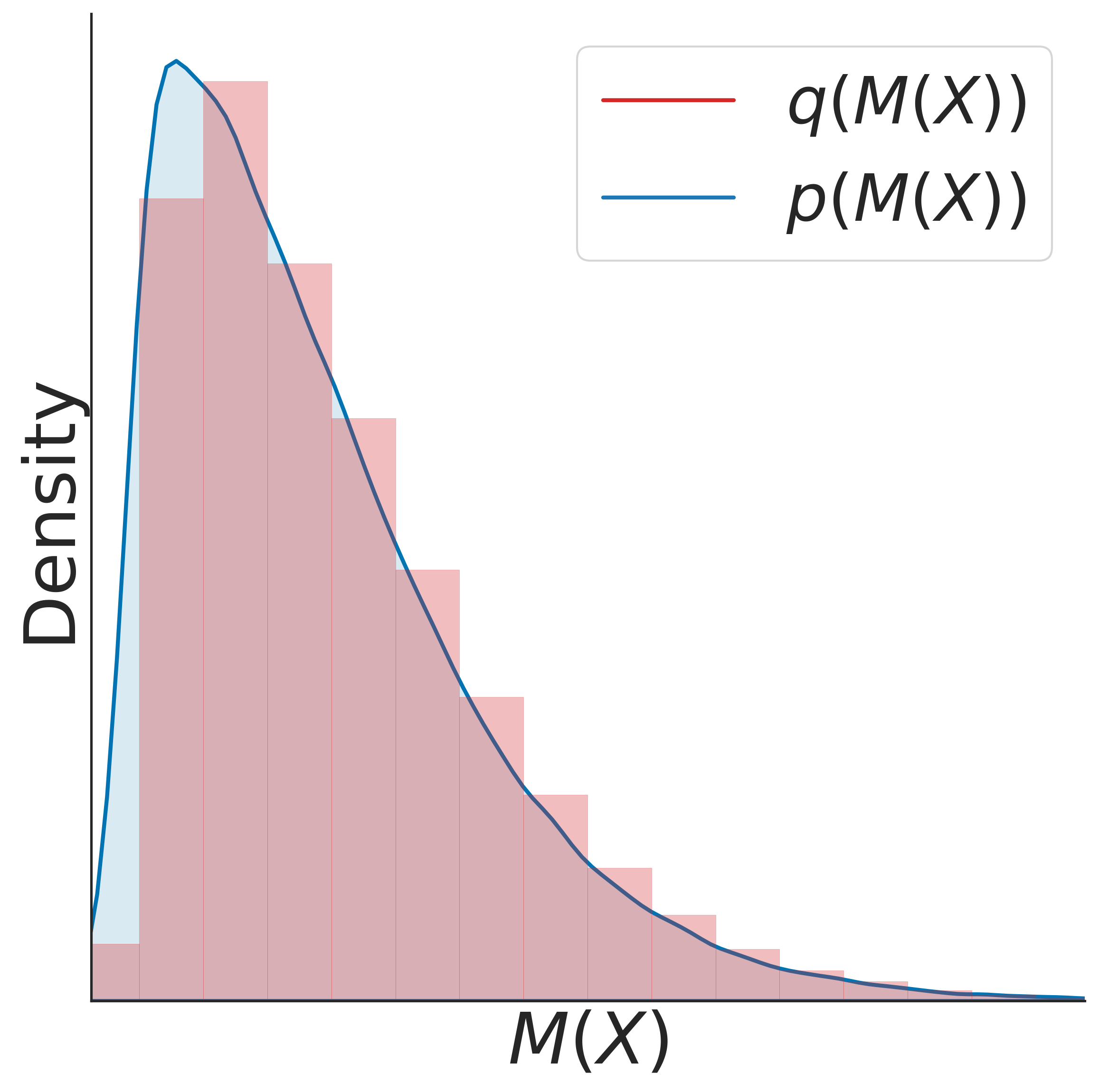
(d) VIC $q(M(X))$

Figure 9: VIC improves compression of Banana distribution when downstream tasks are invariant to translation on the $y$-axis by (implicitly) estimating the density $p(M(X))$. (a) standard compression with a rate of $4.86$ bits and an invariant distortion of $7.67\text{e-}2$ ; (b) the induced marginal distribution $q(M(X))$ of the $x$-value of the reconstructions from the standard neural compressor; (c) our compression with a rate of $3.24$ bits and an invariant distortion of $7.84\text{e-}2$. (b) the induced marginal distribution $q(M(X))$ of the $x$-value of the reconstructions from the VIC;

$y$-translation and induced distribution

Fig. 9 considers the case where downstream tasks are invariant to $y$-translations. In this case the maximal invariant used during training is chosen to be $M:x\mapsto[0,x_{2}]^{T}$. Similarly to the case of $x$-translation and rotations, we see that our model can perform as well as a standard compressor for a fraction of the rate.

To provide a better intuition as to why this is the case we also plot the distribution of the reconstructions when marginalized over the $y$-axis. In other words we plot the distribution of $M(X)$ when applied to the reconstructions, i.e., the $x$ component of the reconstructions. We see that although the partition of the source space is very different for a standard compressor (Fig. 9(a)) and for our VIC (Fig. 9(c)), the induced distribution (and partition) in the marginalized space are actually very similar (Fig. 9(b) and Fig. 9(d)). This shows where our bit-rate gains come from. Indeed from Prop. 1 we know that in the case of invariant tasks one only needs to model the distribution of $M(X)$ (e.g. the distribution of the $x$ component here), and we see that both the standard compressor and VIC does that similarly well. The main difference being that VIC does so in an optimal way while the standard compressor needs to partition the input space in a finer way to achieve a similar induced partition in the $M(X)$ space.

What is the relation between rate and predictions? Theorem 2 shows that, for log loss, the minimum rate is linearly related to the loss $\delta$ in downstream performance. Our theory (Sec. B.6) suggests a logarithmic relationship for MSE. This is seen for VIC and VC in Fig. 4 of the main text (log scale $x$-axis).

On lossy compression and equivalences

Efficient lossy compression is about learning a partition (e.g. Voronoi diagrams, or Fig. 8 ) of the input space to map many inputs to the same code. We use the fact that any partition can be constructed from an equivalence relation [150] to learn compressors that are invariant to desired transformations. The shape of the partitions are then induced by the transformations, which perturb points in their quantization bins (equivalence classes), e.g., rotations in Fig. 4 of the main text. The size of the partition, e.g., disks width in Fig. 4 of the main text, depend on the desired performance $\delta$. The pink dots are representatives of the partition, i.e., maximal invariants. The key is that using our objectives we can learn arbitrary quantization using only desired transformations, which ML practictioners already use for data augmentations.

F.2 MNIST

(a) Rate-Error

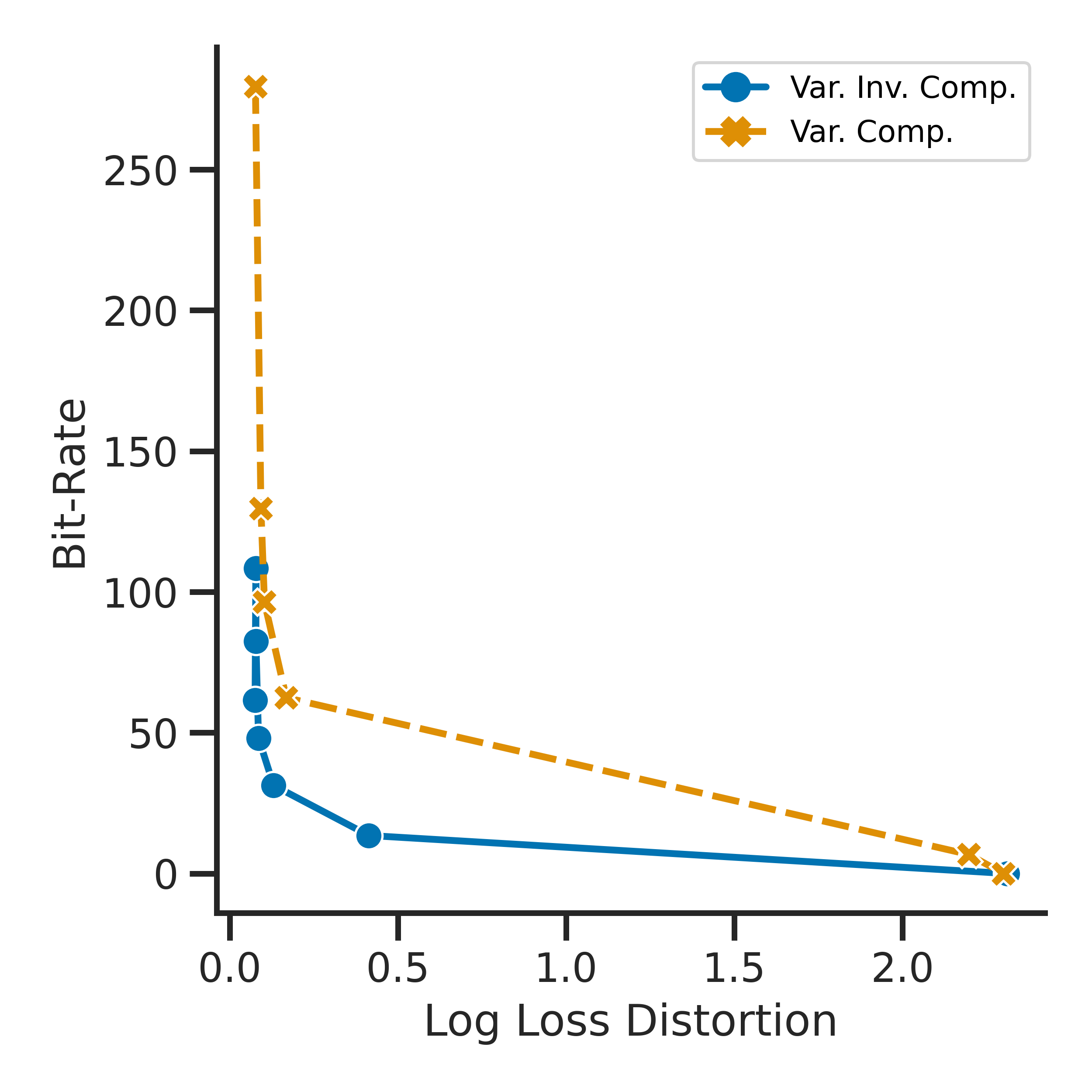
(b) Rate-Log loss

Figure 10: Augmented MNIST RD curves for downstream predictions are very similar when using classification error (left) instead of the log loss (right) from our theory.

How do RD curves change if we use classification error instead of log loss? Our theory Theorem 2 only ensures good downstream log loss risk. Nevertheless, we used here the classification error ($1-\text{accuracy}$) throughout the main test as it is more commonly used for evaluating classification performance. Fig. 10 shows that RD curves are very similar for when using classification error instead of accuracy. This is not very surprising as log loss is the standard (differential) proxy of classification error in ML.

Table 6: Using label-preserving augmentations that remove more information about $X$ decreases the rate without hindering classification performance. Single run.

	Augmentations	Rate $[\frac{\text{bits}}{\text{img}}]$	Test Acc. $[\%]$
VIC	Small set	$185.3$	$96.2$
	Large set	$79.0$	$97.9$
	Supervised (largest set)	$5.7$	$99.1$
BINCE	Small set	$256$	$95.3$
	Large set	$131$	$97.8$
	Supervised (largest set)	$5.9$	$97.8$

What is the impact of the choice of augmentations? The rate decreases when $A$ removes more information from $X$. Indeed, we have $\operatorname{I}\negthinspace\left[X;A(X)\right]=\operatorname{I}\negthinspace\left[X;M(X)\right]+\operatorname{I}\negthinspace\left[X;M(X)\right]=\operatorname{I}\negthinspace\left[X;M(X)\right]+0=\operatorname{H}\negthinspace\left[M(X)\right]$, where the second equality comes from Assumption 7 and the last equality from the determinism of $M$. As a result we can rewrite Theorem 2 as $Rate(\delta)=\operatorname{I}\negthinspace\left[X;A(X)\right]-\delta$. To illustrate this we trained our VIC and BINCE using three augmentation sets on MNIST, all of which keep the true label invariant but progressively discard more $X$ information: 1 standard image augmentations such as random translations, shears, and rescalings; 2 those same standard image augmentations, but drawn from larger ranges of possible translations, shears, scales, etc; 3 supervised “augmentations” line in [151] that remove everything except label information, i.e., for every image $x$ let $x^{+}=A(x)$ be a random image with the same label. Table 6 shows that using label-preserving augmentations that remove more information about $X$ greatly decreases the rate without hindering classification performance. The fact that the supervised augmentations achieve a much better rate, shows that typical SSL compression is still very far from single-task label compression. SSL compression retains information for at least $2^{79}\approx 10^{23}$ disjoint labels.

Table 7: End-to-end compression of augmented MNIST works much better than staggered compression for both VIC and BINCE. Single run.

		Rate $[\frac{\text{bits}}{\text{img}}]$	Test Acc. $[\%]$
VIC	Staggered	$477$	$98.0$
	End-to-end	$79$	$97.9$
BINCE	Staggered	$358$	$97.4$
	End-to-end	$131$	$97.8$

How much does end-to-end improve compared to staggered training? We evaluated end-to-end training for both our losses against a staggered version that consists in first optimizing the distortion and then adding an entropy bottleneck to performing lossy compression of the learned representations (as in Sec. 5.3). Table 7 shows that end-to-end training can give large gains compared to the staggered method and that our compression gains with CLIP could be even further improved.

F.3 STL10

In the main text we used the STL10 data set to answer some principled questions about our method in controlled experiments. We provide additional results here.

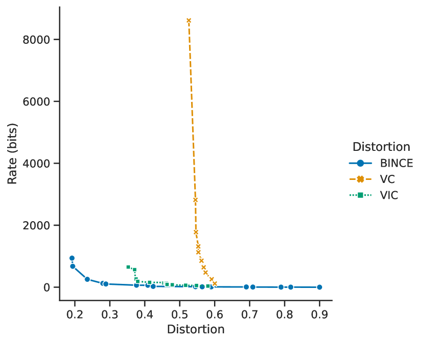
(a) From features $\hat{Z}$

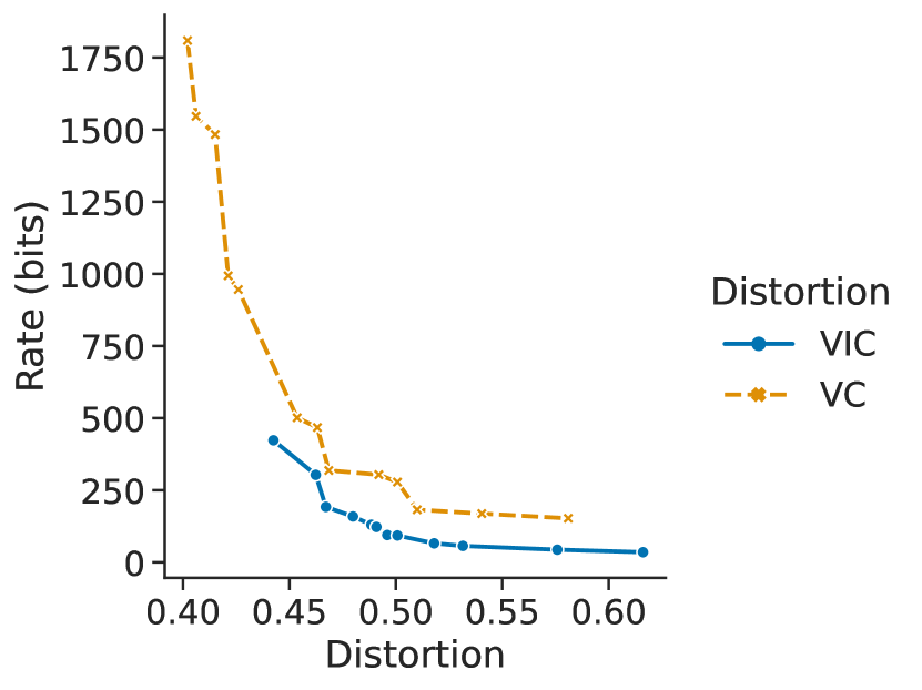
(b) From reconstruction $\hat{X}$

Figure 11: BINCE achieves the best RI curves followed by VIC and then VC for STL10 data. Rate-error curves when predicting downstream tasks from: (left) compressed representations $\hat{Z}$, (right) reconstructions $\hat{X}$.

How does the choice of distortion measures or bounds thereof affect RI curves? Supplementing the results in the main text, we show more extensive results comparing the effect of the distortion measures (invariant or not) or bounds thereof (BINCE and VIC are different bounds on $\operatorname{R}\negthinspace\left[M(X)\,|\,Z\right]$) on RI curves. When predicting from compressed representations $\hat{Z}$ (Fig. 11 left), BINCE achieves the best RI curves followed by VIC and VC. When predicting from reconstructions $\hat{X}$ (Fig. 11 right), VIC still performs a little better than VC although the gap shrinks. Table 1 shows all quantitative results for best achieved downstream performance (as in Table 1 from the main text).

Table 8: We compare classical compression formats (PNG, JPEG, webP) to neural (VC) and invariant (BINCE, VIC) ones. BINCE achieves the same error rate but compresses $121.1\times$ better.

Distortion	Predict from	Best error $[\%]$	Rate [Mb/img]	Compression factor
PNG [38]	reconstructions	19.2	14.20	$1\times$
JPEG [39]	reconstructions	19.9	4.60	$3.0\times$
WebP [40]	reconstructions	20.3	1.12	$12.7\times$
VC	reconstructions	40.2	0.23	$62.8\times$
VC	features	52.6	1.08	$13.2\times$
VIC (ours)	reconstructions	44.3	0.05	$268.6\times$
VIC (ours)	features	35.3	0.08	$174.8\times$
BINCE (ours)	features	19.2	0.12	$121.1\times$

Note that VIC and VC achieve much worst downstream performance than BINCE. Based on preliminary results, we believe that this comes from the fact that, for consistency, in all experiments we used ResNet18 encoders. Indeed, ResNet18 have an global averaging pooling layer that averages the “latent image” over spatial dimensions (width and height). As a result, the representations $\hat{Z}$ does not retain any spatial information, which is often useful for improving reconstructions. Preliminary results showed that removing this pooling layer improves downstream predictions significantly. Importantly, this impacts both VIC and VC so although the absolute performance improved by removing this layer the relative error did not seem to.

For all our models the we estimated (using a naive sample estimate) the mutual information $\operatorname{I}\negthinspace\left[Z;Y\right]$ and found that $\hat{\mathrm{I}}\negthinspace\left[Z,X\right]=\hat{\mathrm{H}}\negthinspace\left[Y\right]$. This shows that all information about labels is retained, i.e., no images get compressed to the same Z but have different labels. The difference in test accuracy (which is also similar for training) must thus come from the fact that some information is easier to use/decode from [52, 51]. Indeed, our framework only concerns information retention rather than information usability. This is further supported by the fact that BINCE gets very good downstream accuracy, because it has been shown in theory [29, 30, 31] and in practice [32, 15] that contrastive representations are approximately linearly decodable.

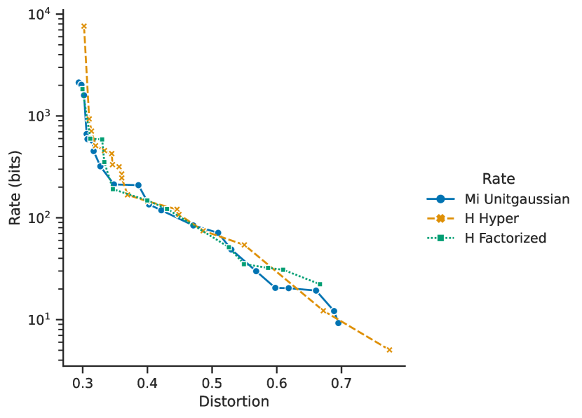
Figure 12: The choice of variational bounds on the rate term $\operatorname{I}\negthinspace\left[Z;X\right]$ has little effect on RI curves for STL10 data. “MI unitgaussian” is the upper bound on mutual information used in VIB and VAE; “H factorized” is Ballé et al.’s [28] upper bound on $\operatorname{H}\negthinspace\left[Z\right]$ with a factorized entropy model; “H hyper” is Ballé et al.’s [28] upper bound on $\operatorname{H}\negthinspace\left[Z\right]$ with a hyperprior entropy model.

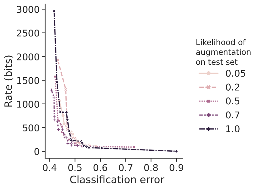
Figure 13: VIC is robust to distribution shifts in the augmentations as it is invariant to the augmentations. Specifically, test time shifts in augmentation probability seem to have little effect on the rate-distortion curve for the case of STL10 data.

Table 9: Hierarchical hyperprior works worst (higher rates) for low distortion, when compared to a factorized prior and a mutual information bottleneck on STL10 data.

Bottleneck	Entropy model	Lossless Rate [bits/img]	Lossless loss
Entropy $\operatorname{H}\negthinspace\left[Z\right]$	Factorized prior [28]	598.5	0.3117
Entropy $\operatorname{H}\negthinspace\left[Z\right]$	Hierarchical prior [28]	934.7	0.3100
Mutual Information $\operatorname{I}\negthinspace\left[Z;X\right]$	Unit Gaussian	592.5	0.3074

How does the choice of bounds on the rate term $\operatorname{I}\negthinspace\left[Z;X\right]$ impact RI curves? For the main paper we always used the standard [24] neural compressor’s upper bound on $\operatorname{I}\negthinspace\left[Z;X\right]$, namely, the entropy bound $\operatorname{I}\negthinspace\left[Z;X\right]\leq\operatorname{H}\negthinspace\left[Z\right]\leq\operatorname{E}_{p(Z,X)}\negthinspace\left[q_{\theta}(Z)\right]$. To understand the effect of using other bounds on $\operatorname{I}\negthinspace\left[Z;X\right]$ and different entropy models $q_{\theta}(Z)$. Specifically, in Fig. 13 we compare three different bounds on mutual information: (MI unitgaussian) the mutual information bound from VAE and VIB $\operatorname{I}\negthinspace\left[Z;X\right]\leq\operatorname{D}_{\text{KL}}\negthinspace\left[p_{\varphi}(Z|X)\right]{q_{\theta}(Z)}$; (H Factorized) the entropy bound $\operatorname{H}\negthinspace\left[Z\right]\leq\operatorname{E}_{p(Z,X)}\negthinspace\left[q_{\theta}(Z)\right]$ where $q_{\theta}(Z)$ is Ballé et al.’s [28] factorized entropy model; (H Hyper) the entropy bound where $q_{\theta}(Z)$ is Ballé et al.’s [28] hyperprior entropy model. In our experiments, however, we find that neither of these choices influence the RD curves at typical distortion levels as seen Fig. 13. In our experiments we use “H Hyper”, which does seem to enable very low rates (high distortions) but seems to perform worst at very high rates (see Table 9)

How important is the distribution over augmentations? As discussed in the main text, RD curves of our VIC show negligible difference when the distribution of augmentation shifts from training to test time. We provide this evidence in Fig. 13. Here we trained a VIC compressor on data with various augmentations, if these were (jointly) applied or not would be decided by a fair coin flip. At test time, we changed the coin to be biased with $p=0.05,0.2,0.5,0.7,1.0$.

F.4 Pretrained CLIP

Table 10: Converting a pretrained SSL model into a zero-shot compressor achieves substantial bit-rate gains while allowing test accuracies similar to predicting from raw images. CLIP refers to the original CLIP with lossless compression of the representations. CLIP+EB refers to our CLIP compressor. CLIP+EB^$-$ and CLIP+EB^$+$ are our CLIP compressors trained respectively for a larger and smaller bit-rate. We provide downstream evaluation using an MLP and a linear (SVM) predictor. Baselines: JPEG and compression of features from a ImageNet pretrained classifier (Transfer + EB).

			ImageNet	STL	PCam	Cars	CIFAR10	CIFAR100	Food	Pets	Caltech
Rate [Bits/img]		JPEG	1.49e6	4.71e4	9.60e4	1.92e5	1.05e4	1.05e4	1.54e5	1.81e5	1.69e5
		Transfer + EB	3.95e3	3.33e3	3.99e3	3.18e3	3.92e3		3.26e3	3.70e3	3.40e3
		CLIP	1.52e4	1.52e4	1.52e4	1.52e4	1.52e4	1.52e4	1.52e4	1.52e4	1.52e4
		CLIP+EB$-$	2.47e3	2.46e3	2.61e3	2.59e3	2.53e3	2.54e3	2.39e3	2.33e3	2.46e3
		CLIP+EB	1.35e3	1.34e3	1.49e3	1.47e3	1.41e3	1.42e3	1.27e3	1.21e3	1.34e3
		CLIP+EB$+$	9.63e2	9.52e2	1.49e3	1.52e2	1.02e2	1.09e3	8.89e2	8.35e2	9.53e2
Test Accuracies $[\%]$	[41]	JPEG	76.6	99.0	82.6	49.1	96.7	86.3	81.8	90.4	94.5
		CLIP [41]	76.1	98.3	83.9	81.8	95.1	80.5	88.8	90.0	93.0
	MLP	Transfer + EB	72.7	96.1	79.4	42.0	87.0		66.8	91.3	89.9
		CLIP	76.5	98.6	84.5	80.8	95.3	80.9	88.5	89.7	93.2
		CLIP+EB$-$	76.6	98.7	82.7	80.4	95.3	80.9	88.5	89.6	93.5
		CLIP+EB	76.3	98.7	80.9	79.6	95.2	80.1	88.3	89.5	93.4
		CLIP+EB$+$	76.0	98.7	80.1	78.9	94.8	78.6	87.6	88.6	92.9
	Linear	CLIP		98.6	83.8	80.8	95.0	79.8	85.0	89.3	93.8
		CLIP+EB$-$		98.7	83.2	80.8	95.0	79.7	85.0	89.2	93.6
		CLIP+EB		98.7	81.1	79.9	94.8	79.0	83.6	88.3	93.7
		CLIP+EB$+$		98.6	80.5	78.9	94.4	80.5	82.5	87.8	93.5

In Table 10 we provide all the quantitative results for our zero-shot CLIP experiments from which we derived the tables in the main text.

We note that zero-shot compression can still be analysed using our framework. Indeed CLIP was trained on $400M$ sampled from a r.v. $X$ over images on the internet. As these datasets are on internet, they are samples from the joint $(X,Y)$ for a specific task $Y$. One can see this as a multi-task setting (each dataset is a distinct task).

What is the effect of using a more powerful predictor from the representation? In our framework we only discuss about information but never whether this information can easily be decoded by the predictors of interest. We investigated the effect of using more powerful predictors from our representation to understand how easy it is to decode the information in our representation. In particular, we evaluated all our CLIP compressors (i.e. at different $\beta$), by considering predictions from our compressed representation using a two layer MLP and using a linear classifier (SVM). Table 10 shows that the advantage of using an MLP compared to a linear model is small, which suggests that our CLIP compressed representation store information in a way that is easily decodable. This is typical from contrastive self-supervised models [15, 32].

How does compressing SSL compare to compressing features form transfer learning? In previous work, Singh et al. [50] had considered the case of compressing features from single-task transfer learning instead of self-supervised method. In Table 10 we compare compression of both type of features. Specifically “Transfer + EB” shows compression of a pretrained ResNet50 on ImageNet. We see that It generally performs worst than our CLIP compressor both in terms of test accuracies and bit-rate. One issue with this comparison is that the architectures of both models are not the same is likely that “transfer+EB” does not even perform better than CLIP on ImageNet.

F.5 Galaxy Zoo

Table 11: Comparisons between pretrained CLIP BINCE, a BINCE trained end-to-end, and SOTA perceptual compressors on Galaxyzoo data. CLIP BINCE achieves the smallest bit-rate.

Compressor	rate	test loss	val. loss mean	median	max	min	std
	$[\text{Mb/img}]$	$[\text{ }]$	$[\text{ }]$	$[10^{-3}]$	$[\text{ }]$	$[10^{-7}]$	$[10^{-2}]$
PNG	53.73	0.007	0.008	0.86	0.07	1.04	1.62
JPEG	1.68	0.012	0.013	1.25	0.11	1.23	2.61
WebP	0.48	0.010	0.011	1.20	0.10	1.16	2.29
BINCE (CLIP)	0.33	0.011	0.011	1.13	0.10	7.59	2.29
BINCE (end to end)	1.77	0.012	0.012	1.43	0.11	1.31	2.50

Humanity observes earth and sky at high temporal and spatial resolution, this can easily fill entire data centers. What is more, multiple copies of these series often exist over the world. At recording time it is usually not clear what kind of queries need to be answered about the recordings in the future; What was the weather like 10 years ago? Did a glacier resolve here? ect. To investigate our method in such real world scenario we compressed the GalaxyZoo telescope dataset (GZ2) and its 37 classification tasks. In Table 11, we compare a classical lossless and lossy method, to our BINCE at same distortions.

How well does CLIP pretraining work compared to in domain training? In the main paper we have seen that CLIP pretraining gives rise to a compressor that generalizes very well across different datasets. We evaluated how well the CLIP compressor generalizes compare to training BINCE directly end-to-end on GZ2’s training set. Table 11 shows that the CLIP compressor works much better ($4\times$ rate gains) than the end-to-end BINCE. This suggests that pretraining can really be beneficial for training invariant compressors, and that our CLIP compressor can generalize very well across datasets.

How does our CLIP compressor generalize to very different images compared to SOTA compressors? In the main text we have seen that our CLIP compressor generalizes very well across different datasets compared to high quality JPEG. To better understand the limits of the generalization capacity of our CLIP compressor, we compared it to a SOTA classical compressor (WebP) on images that are completely different than the ones CLIP was trained on, namely Galaxy images (not typical images on internet). We see in Table 11 that in this challenging setting our CLIP compressor only achieves relatively small gains ($30\%$).

References

- Rolnick et al. [2019] D. Rolnick, P. L. Donti, L. H. Kaack, K. Kochanski, A. Lacoste, K. Sankaran, A. S. Ross, N. Milojevic-Dupont, N. Jaques, A. Waldman-Brown, A. Luccioni, T. Maharaj, E. D. Sherwin, S. K. Mukkavilli, K. P. Körding, C. P. Gomes, A. Y. Ng, D. Hassabis, J. C. Platt, F. Creutzig, J. T. Chayes, and Y. Bengio, “Tackling Climate Change with Machine Learning,” CoRR, vol. abs/1906.05433, 2019, _eprint: 1906.05433. [Online]. Available: http://arxiv.org/abs/1906.05433
- Zgurovsky and Zaychenko [2020] M. Z. Zgurovsky and Y. P. Zaychenko, Big Data: Conceptual Analysis and Applications. Springer, 2020.
- Kalra and Paddock [2016] N. Kalra and S. M. Paddock, “Driving to safety: How many miles of driving would it take to demonstrate autonomous vehicle reliability?” Transportation Research Part A: Policy and Practice, vol. 94, pp. 182–193, 2016, publisher: Elsevier.
- Yeong et al. [2021] D. J. Yeong, G. Velasco-Hernandez, J. Barry, J. Walsh, and others, “Sensor and sensor fusion technology in autonomous vehicles: a review,” Sensors, vol. 21, no. 6, p. 2140, 2021, publisher: Multidisciplinary Digital Publishing Institute.
- Johnston [1988] J. Johnston, “Transform coding of audio signals using perceptual noise criteria,” IEEE Journal on Selected Areas in Communications, vol. 6, no. 2, pp. 314–323, Feb. 1988, conference Name: IEEE Journal on Selected Areas in Communications.
- Heeger and Teo [1995] D. J. Heeger and P. C. Teo, “A model of perceptual image fidelity,” in Proceedings 1995 International Conference on Image Processing, Washington, DC, USA, October 23-26, 1995. IEEE Computer Society, 1995, pp. 343–345. [Online]. Available: https://doi.org/10.1109/ICIP.1995.537485
- Lee and Ebrahimi [2012] J.-S. Lee and T. Ebrahimi, “Perceptual Video Compression: A Survey,” Ieee Journal Of Selected Topics In Signal Processing, vol. 6, no. 6, p. 684, 2012, number: ARTICLE Publisher: Ieee-Inst Electrical Electronics Engineers Inc. [Online]. Available: https://infoscience.epfl.ch/record/184275
- Blau and Michaeli [2019] Y. Blau and T. Michaeli, “Rethinking Lossy Compression: The Rate-Distortion-Perception Tradeoff,” in Proceedings of the 36th International Conference on Machine Learning, ICML 2019, 9-15 June 2019, Long Beach, California, USA, ser. Proceedings of Machine Learning Research, K. Chaudhuri and R. Salakhutdinov, Eds., vol. 97. PMLR, 2019, pp. 675–685. [Online]. Available: http://proceedings.mlr.press/v97/blau19a.html
- Pan [1993] Y. Pan, “Digital Audio Compression,” Digital Technical Journal, 1993.
- Mentzer et al. [2020] F. Mentzer, G. Toderici, M. Tschannen, and E. Agustsson, “High-Fidelity Generative Image Compression,” in Advances in Neural Information Processing Systems 33: Annual Conference on Neural Information Processing Systems 2020, NeurIPS 2020, December 6-12, 2020, virtual, H. Larochelle, M. Ranzato, R. Hadsell, M.-F. Balcan, and H.-T. Lin, Eds., 2020. [Online]. Available: https://proceedings.neurips.cc/paper/2020/hash/8a50bae297807da9e97722a0b3fd8f27-Abstract.html
- Tishby et al. [2000] N. Tishby, F. C. N. Pereira, and W. Bialek, “The information bottleneck method,” CoRR, vol. physics/0004057, 2000. [Online]. Available: http://arxiv.org/abs/physics/0004057
- Heaton [2018] J. Heaton, “Ian Goodfellow, Yoshua Bengio, and Aaron Courville: Deep learning - The MIT Press, 2016, 800 pp, ISBN: 0262035618,” Genet. Program. Evolvable Mach., vol. 19, no. 1-2, pp. 305–307, 2018. [Online]. Available: https://doi.org/10.1007/s10710-017-9314-z
- Shorten and Khoshgoftaar [2019] C. Shorten and T. M. Khoshgoftaar, “A survey on Image Data Augmentation for Deep Learning,” Journal of Big Data, vol. 6, no. 1, p. 60, Jul. 2019. [Online]. Available: https://doi.org/10.1186/s40537-019-0197-0
- Kingma and Welling [2014] D. P. Kingma and M. Welling, “Auto-Encoding Variational Bayes,” in 2nd International Conference on Learning Representations, ICLR 2014, Banff, AB, Canada, April 14-16, 2014, Conference Track Proceedings, Y. Bengio and Y. LeCun, Eds., 2014. [Online]. Available: http://arxiv.org/abs/1312.6114
- Oord et al. [2019] A. v. d. Oord, Y. Li, and O. Vinyals, “Representation Learning with Contrastive Predictive Coding,” arXiv:1807.03748 [cs, stat], Jan. 2019, arXiv: 1807.03748. [Online]. Available: http://arxiv.org/abs/1807.03748
- Deng et al. [2009] J. Deng, W. Dong, R. Socher, L.-J. Li, K. Li, and L. Fei-Fei, “ImageNet: A large-scale hierarchical image database,” in 2009 IEEE Conference on Computer Vision and Pattern Recognition, Jun. 2009, pp. 248–255, iSSN: 1063-6919.
- Shannon [1959] C. E. Shannon, “Coding theorems for a discrete source with a fidelity criterion,” IRE Nat. Conv. Rec, vol. 4, no. 142-163, p. 1, 1959.
- Berger [1968] T. Berger, “Rate distortion theory for sources with abstract alphabets and memory,” Information and Control, vol. 13, no. 3, pp. 254–273, Sep. 1968. [Online]. Available: https://linkinghub.elsevier.com/retrieve/pii/S0019995868911236
- Eaton [1989] M. L. Eaton, “Group Invariance Applications in Statistics,” Regional Conference Series in Probability and Statistics, vol. 1, pp. i–133, 1989, publisher: Institute of Mathematical Statistics. [Online]. Available: https://www.jstor.org/stable/4153172
- Rashevsky [1955] N. Rashevsky, “Life, information theory, and topology,” The bulletin of mathematical biophysics, vol. 17, no. 3, pp. 229–235, Sep. 1955. [Online]. Available: https://doi.org/10.1007/BF02477860
- Varshney and Goyal [2007] L. R. Varshney and V. K. Goyal, “Benefiting from Disorder: Source Coding for Unordered Data,” arXiv:0708.2310 [cs, math], Aug. 2007, arXiv: 0708.2310. [Online]. Available: http://arxiv.org/abs/0708.2310
- Kolchinsky et al. [2019] A. Kolchinsky, B. D. Tracey, and S. V. Kuyk, “Caveats for information bottleneck in deterministic scenarios,” in 7th International Conference on Learning Representations, ICLR 2019, New Orleans, LA, USA, May 6-9, 2019. OpenReview.net, 2019. [Online]. Available: https://openreview.net/forum?id=rke4HiAcY7
- Bottou [2010] L. Bottou, “Large-Scale Machine Learning with Stochastic Gradient Descent,” in 19th International Conference on Computational Statistics, COMPSTAT 2010, Paris, France, August 22-27, 2010 - Keynote, Invited and Contributed Papers, Y. Lechevallier and G. Saporta, Eds. Physica-Verlag, 2010, pp. 177–186. [Online]. Available: https://doi.org/10.1007/978-3-7908-2604-3_16
- Ballé et al. [2017] J. Ballé, V. Laparra, and E. P. Simoncelli, “End-to-end Optimized Image Compression,” in 5th International Conference on Learning Representations, ICLR 2017, Toulon, France, April 24-26, 2017, Conference Track Proceedings. OpenReview.net, 2017. [Online]. Available: https://openreview.net/forum?id=rJxdQ3jeg
- Theis et al. [2017] L. Theis, W. Shi, A. Cunningham, and F. Huszár, “Lossy Image Compression with Compressive Autoencoders,” in 5th International Conference on Learning Representations, ICLR 2017, Toulon, France, April 24-26, 2017, Conference Track Proceedings. OpenReview.net, 2017. [Online]. Available: https://openreview.net/forum?id=rJiNwv9gg
- Rissanen [1976] J. J. Rissanen, “Generalized Kraft Inequality and Arithmetic Coding,” IBM Journal of Research and Development, vol. 20, no. 3, pp. 198–203, May 1976, conference Name: IBM Journal of Research and Development.
- Duda [2009] J. Duda, “Asymmetric numeral systems,” CoRR, vol. abs/0902.0271, 2009, _eprint: 0902.0271. [Online]. Available: http://arxiv.org/abs/0902.0271
- Ballé et al. [2018] J. Ballé, D. Minnen, S. Singh, S. J. Hwang, and N. Johnston, “Variational image compression with a scale hyperprior,” in 6th International Conference on Learning Representations, ICLR 2018, Vancouver, BC, Canada, April 30 - May 3, 2018, Conference Track Proceedings. OpenReview.net, 2018. [Online]. Available: https://openreview.net/forum?id=rkcQFMZRb
- Saunshi et al. [2019] N. Saunshi, O. Plevrakis, S. Arora, M. Khodak, and H. Khandeparkar, “A Theoretical Analysis of Contrastive Unsupervised Representation Learning,” in Proceedings of the 36th International Conference on Machine Learning, ICML 2019, 9-15 June 2019, Long Beach, California, USA, ser. Proceedings of Machine Learning Research, K. Chaudhuri and R. Salakhutdinov, Eds., vol. 97. PMLR, 2019, pp. 5628–5637. [Online]. Available: http://proceedings.mlr.press/v97/saunshi19a.html
- Tosh et al. [2021] C. Tosh, A. Krishnamurthy, and D. Hsu, “Contrastive learning, multi-view redundancy, and linear models,” in Algorithmic Learning Theory, 16-19 March 2021, Virtual Conference, Worldwide, ser. Proceedings of Machine Learning Research, V. Feldman, K. Ligett, and S. Sabato, Eds., vol. 132. PMLR, 2021, pp. 1179–1206. [Online]. Available: http://proceedings.mlr.press/v132/tosh21a.html
- Lee et al. [2020] J. D. Lee, Q. Lei, N. Saunshi, and J. Zhuo, “Predicting What You Already Know Helps: Provable Self-Supervised Learning,” arXiv:2008.01064 [cs, stat], Aug. 2020, arXiv: 2008.01064. [Online]. Available: http://arxiv.org/abs/2008.01064
- Chen et al. [2020a] T. Chen, S. Kornblith, M. Norouzi, and G. E. Hinton, “A Simple Framework for Contrastive Learning of Visual Representations,” in Proceedings of the 37th International Conference on Machine Learning, ICML 2020, 13-18 July 2020, Virtual Event, ser. Proceedings of Machine Learning Research, vol. 119. PMLR, 2020, pp. 1597–1607. [Online]. Available: http://proceedings.mlr.press/v119/chen20j.html
- Poole et al. [2019] B. Poole, S. Ozair, A. v. d. Oord, A. Alemi, and G. Tucker, “On Variational Bounds of Mutual Information,” in Proceedings of the 36th International Conference on Machine Learning, ICML 2019, 9-15 June 2019, Long Beach, California, USA, ser. Proceedings of Machine Learning Research, K. Chaudhuri and R. Salakhutdinov, Eds., vol. 97. PMLR, 2019, pp. 5171–5180. [Online]. Available: http://proceedings.mlr.press/v97/poole19a.html
- Song and Ermon [2020] J. Song and S. Ermon, “Multi-label Contrastive Predictive Coding,” arXiv:2007.09852 [cs, stat], Jul. 2020, arXiv: 2007.09852. [Online]. Available: http://arxiv.org/abs/2007.09852
- He et al. [2016] K. He, X. Zhang, S. Ren, and J. Sun, “Deep Residual Learning for Image Recognition,” in 2016 IEEE Conference on Computer Vision and Pattern Recognition (CVPR). Las Vegas, NV, USA: IEEE, Jun. 2016, pp. 770–778. [Online]. Available: http://ieeexplore.ieee.org/document/7780459/
- Ballé et al. [2020] J. Ballé, P. A. Chou, D. Minnen, S. Singh, N. Johnston, E. Agustsson, S. J. Hwang, and G. Toderici, “Nonlinear Transform Coding,” CoRR, vol. abs/2007.03034, 2020, _eprint: 2007.03034. [Online]. Available: https://arxiv.org/abs/2007.03034
- Coates et al. [2011] A. Coates, A. Ng, and H. Lee, “An analysis of single-layer networks in unsupervised feature learning,” in Proceedings of the fourteenth international conference on artificial intelligence and statistics. JMLR Workshop and Conference Proceedings, 2011, pp. 215–223.
- Graphics [PNG] P. N. Graphics (PNG), ISO/IEC 15948, 2003, published: hhttp://www.libpng.org/pub/png/spec/iso/index-object.html.
- Group [JPEG] J. P. E. Group (JPEG), ITU-T T.81, ITU-T T.83, ITU-T T.84, ITU-T T.86, ISO/IEC 10918, 1992, published: www.jpeg.org/jpeg/.
- WebP [2018] WebP, Google, 2018, published: developers.google.com/speed/webp.
- Radford et al. [2021] A. Radford, J. W. Kim, C. Hallacy, A. Ramesh, G. Goh, S. Agarwal, G. Sastry, A. Askell, P. Mishkin, J. Clark, G. Krueger, and I. Sutskever, “Learning Transferable Visual Models From Natural Language Supervision,” arXiv:2103.00020 [cs], Feb. 2021, arXiv: 2103.00020. [Online]. Available: http://arxiv.org/abs/2103.00020
- Dosovitskiy et al. [2020] A. Dosovitskiy, L. Beyer, A. Kolesnikov, D. Weissenborn, X. Zhai, T. Unterthiner, M. Dehghani, M. Minderer, G. Heigold, S. Gelly, J. Uszkoreit, and N. Houlsby, “An Image is Worth 16x16 Words: Transformers for Image Recognition at Scale,” CoRR, vol. abs/2010.11929, 2020, _eprint: 2010.11929. [Online]. Available: https://arxiv.org/abs/2010.11929
- Lin et al. [2015] T.-Y. Lin, M. Maire, S. Belongie, L. Bourdev, R. Girshick, J. Hays, P. Perona, D. Ramanan, C. L. Zitnick, and P. Dollár, “Microsoft COCO: Common Objects in Context,” arXiv:1405.0312 [cs], Feb. 2015, arXiv: 1405.0312. [Online]. Available: http://arxiv.org/abs/1405.0312
- Veeling et al. [2018] B. S. Veeling, J. Linmans, J. Winkens, T. Cohen, and M. Welling, “Rotation Equivariant CNNs for Digital Pathology,” arXiv:1806.03962 [cs, stat], Jun. 2018, arXiv: 1806.03962. [Online]. Available: http://arxiv.org/abs/1806.03962
- Liu et al. [2018] Z. Liu, T. Liu, W. Wen, L. Jiang, J. Xu, Y. Wang, and G. Quan, “DeepN-JPEG: A Deep Neural Network Favorable JPEG-based Image Compression Framework,” arXiv:1803.05788 [cs], Mar. 2018, arXiv: 1803.05788. [Online]. Available: http://arxiv.org/abs/1803.05788
- Liu et al. [2019a] Z. Liu, X. Xu, T. Liu, Q. Liu, Y. Wang, Y. Shi, W. Wen, M. Huang, H. Yuan, and J. Zhuang, “Machine Vision Guided 3D Medical Image Compression for Efficient Transmission and Accurate Segmentation in the Clouds,” arXiv:1904.08487 [cs, stat], Apr. 2019, arXiv: 1904.08487. [Online]. Available: http://arxiv.org/abs/1904.08487
- Liu et al. [2016] D. Liu, D. Wang, and H. Li, “Recognizable or Not: Towards Image Semantic Quality Assessment for Compression,” Sensing and Imaging, vol. 18, no. 1, p. 1, Dec. 2016. [Online]. Available: https://doi.org/10.1007/s11220-016-0152-5
- Liu et al. [2019b] D. Liu, H. Zhang, and Z. Xiong, “On The Classification-Distortion-Perception Tradeoff,” in Advances in Neural Information Processing Systems 32: Annual Conference on Neural Information Processing Systems 2019, NeurIPS 2019, December 8-14, 2019, Vancouver, BC, Canada, H. M. Wallach, H. Larochelle, A. Beygelzimer, F. d’Alché Buc, E. B. Fox, and R. Garnett, Eds., 2019, pp. 1204–1213. [Online]. Available: https://proceedings.neurips.cc/paper/2019/hash/6c29793a140a811d0c45ce03c1c93a28-Abstract.html
- Weber et al. [2020] M. Weber, C. Renggli, H. Grabner, and C. Zhang, “Observer Dependent Lossy Image Compression,” in Pattern Recognition - 42nd DAGM German Conference, DAGM GCPR 2020, Tübingen, Germany, September 28 - October 1, 2020, Proceedings, ser. Lecture Notes in Computer Science, Z. Akata, A. Geiger, and T. Sattler, Eds., vol. 12544. Springer, 2020, pp. 130–144. [Online]. Available: https://doi.org/10.1007/978-3-030-71278-5_10
- Singh et al. [2020] S. Singh, S. Abu-El-Haija, N. Johnston, J. Ballé, A. Shrivastava, and G. Toderici, “End-to-End Learning of Compressible Features,” in IEEE International Conference on Image Processing, ICIP 2020, Abu Dhabi, United Arab Emirates, October 25-28, 2020. IEEE, 2020, pp. 3349–3353. [Online]. Available: https://doi.org/10.1109/ICIP40778.2020.9190860
- Xu et al. [2020] Y. Xu, S. Zhao, J. Song, R. Stewart, and S. Ermon, “A Theory of Usable Information under Computational Constraints,” in 8th International Conference on Learning Representations, ICLR 2020, Addis Ababa, Ethiopia, April 26-30, 2020. OpenReview.net, 2020. [Online]. Available: https://openreview.net/forum?id=r1eBeyHFDH
- Dubois et al. [2020] Y. Dubois, D. Kiela, D. J. Schwab, and R. Vedantam, “Learning Optimal Representations with the Decodable Information Bottleneck,” in Advances in Neural Information Processing Systems 33: Annual Conference on Neural Information Processing Systems 2020, NeurIPS 2020, December 6-12, 2020, virtual, H. Larochelle, M. Ranzato, R. Hadsell, M.-F. Balcan, and H.-T. Lin, Eds., 2020. [Online]. Available: https://proceedings.neurips.cc/paper/2020/hash/d8ea5f53c1b1eb087ac2e356253395d8-Abstract.html
- Kolmogorov [1956] A. Kolmogorov, “On the Shannon theory of information transmission in the case of continuous signals,” IRE Transactions on Information Theory, vol. 2, no. 4, pp. 102–108, Dec. 1956, conference Name: IRE Transactions on Information Theory.
- Pinsker [1964] M. S. Pinsker, Information and Information Stability of Random Variables and Processes, first edition ed., A. Feinstein, Ed. Holden-Day, Inc., Jan. 1964.
- Jaynes [1957] E. T. Jaynes, “Information Theory and Statistical Mechanics,” Physical Review, vol. 106, no. 4, pp. 620–630, May 1957, publisher: American Physical Society. [Online]. Available: https://link.aps.org/doi/10.1103/PhysRev.106.620
- Lehmann and Romano [2005] E. L. Lehmann and J. P. Romano, Testing statistical hypotheses, 3rd ed., ser. Springer texts in statistics. New York: Springer, 2005.
- Mac Lane and Birkhoff [1999] S. Mac Lane and G. Birkhoff, Algebra. American Mathematical Soc., 1999, google-Books-ID: L6FENd8GHIUC.
- Bloem-Reddy and Teh [2020] B. Bloem-Reddy and Y. W. Teh, “Probabilistic Symmetries and Invariant Neural Networks,” J. Mach. Learn. Res., vol. 21, pp. 90:1–90:61, 2020. [Online]. Available: http://jmlr.org/papers/v21/19-322.html
- Xu and Raginsky [2020] A. Xu and M. Raginsky, “Minimum Excess Risk in Bayesian Learning,” arXiv:2012.14868 [cs, math, stat], Dec. 2020, arXiv: 2012.14868. [Online]. Available: http://arxiv.org/abs/2012.14868
- Kallenberg [2002] O. Kallenberg, “Foundations of Modern Probability,” p. 535, 2002.
- Gneiting and Raftery [2007] T. Gneiting and A. E. Raftery, “Strictly Proper Scoring Rules, Prediction, and Estimation,” Journal of the American Statistical Association, vol. 102, no. 477, pp. 359–378, Mar. 2007. [Online]. Available: http://www.tandfonline.com/doi/abs/10.1198/016214506000001437
- Kraskov et al. [2004] A. Kraskov, H. Stoegbauer, and P. Grassberger, “Estimating Mutual Information,” Physical Review E, vol. 69, no. 6, p. 066138, Jun. 2004, arXiv: cond-mat/0305641. [Online]. Available: http://arxiv.org/abs/cond-mat/0305641
- Berger [1971] T. Berger, Rate Distortion Theory: A Mathematical Basis for Data Compression, ser. Prentice-Hall electrical engineering series. Prentice-Hall, 1971. [Online]. Available: https://books.google.ch/books?id=-HV1QgAACAAJ
- Cover and Thomas [2006] T. M. Cover and J. A. Thomas, Elements of information theory (2. ed.). Wiley, 2006.
- Yongwook Choi and Szpankowski [2009] Yongwook Choi and W. Szpankowski, “Compression of graphical structures,” in 2009 IEEE International Symposium on Information Theory. Seoul, South Korea: IEEE, Jun. 2009, pp. 364–368. [Online]. Available: http://ieeexplore.ieee.org/document/5205736/
- Wu et al. [2019] T. Wu, I. S. Fischer, I. L. Chuang, and M. Tegmark, “Learnability for the Information Bottleneck,” Entropy, vol. 21, no. 10, p. 924, 2019. [Online]. Available: https://doi.org/10.3390/e21100924
- Fischer [2020] I. S. Fischer, “The Conditional Entropy Bottleneck,” Entropy, vol. 22, no. 9, p. 999, 2020. [Online]. Available: https://doi.org/10.3390/e22090999
- Good [1952] I. J. Good, “Rational Decisions,” Journal of the Royal Statistical Society. Series B (Methodological), vol. 14, no. 1, pp. 107–114, 1952, publisher: [Royal Statistical Society, Wiley]. [Online]. Available: https://www.jstor.org/stable/2984087
- Brier [1950] G. W. Brier, “VERIFICATION OF FORECASTS EXPRESSED IN TERMS OF PROBABILITY,” Monthly Weather Review, vol. 78, no. 1, pp. 1–3, Jan. 1950, publisher: American Meteorological Society Section: Monthly Weather Review. [Online]. Available: https://journals.ametsoc.org/view/journals/mwre/78/1/1520-0493_1950_078_0001_vofeit_2_0_co_2.xml
- Good [1971] I. Good, “Comment on “Measuring information and uncertainty” by Robert J. Buehler,” Foundations of Statistical Inference, pp. 337–339, 1971.
- Sriperumbudur et al. [2008] B. K. Sriperumbudur, A. Gretton, K. Fukumizu, G. Lanckriet, and B. Scholkopf, “Injective Hilbert Space Embeddings of Probability Measures,” p. 12, 2008.
- Huszar [2013] F. Huszar, “Scoring rules, Divergences and Information in Bayesian Machine Learning,” Ph.D. dissertation, 2013.
- Gneiting [2010] T. Gneiting, “Making and Evaluating Point Forecasts,” arXiv:0912.0902 [math, stat], Mar. 2010, arXiv: 0912.0902. [Online]. Available: http://arxiv.org/abs/0912.0902
- Shannon [1948] C. E. Shannon, “A mathematical theory of communication,” Bell Syst. Tech. J., vol. 27, no. 4, pp. 623–656, 1948. [Online]. Available: https://doi.org/10.1002/j.1538-7305.1948.tb00917.x
- Jacod and Protter [2004] J. Jacod and P. Protter, Probability Essentials, 2nd ed. Springer-Verlag Berlin Heidelberg, 2004.
- Everett [1963] H. Everett, “Generalized Lagrange Multiplier Method for Solving Problems of Optimum Allocation of Resources,” Operations Research, vol. 11, no. 3, pp. 399–417, Jun. 1963, publisher: INFORMS. [Online]. Available: https://pubsonline.informs.org/doi/abs/10.1287/opre.11.3.399
- Berger [2003] T. Berger, “Rate-Distortion Theory,” in Wiley Encyclopedia of Telecommunications. American Cancer Society, 2003, _eprint: https://onlinelibrary.wiley.com/doi/pdf/10.1002/0471219282.eot142. [Online]. Available: https://onlinelibrary.wiley.com/doi/abs/10.1002/0471219282.eot142
- Paninski [2003] L. Paninski, “Estimation of Entropy and Mutual Information,” Neural Computation, vol. 15, no. 6, pp. 1191–1253, Jun. 2003. [Online]. Available: https://www.mitpressjournals.org/doi/abs/10.1162/089976603321780272
- McAllester and Stratos [2020] D. McAllester and K. Stratos, “Formal Limitations on the Measurement of Mutual Information,” in The 23rd International Conference on Artificial Intelligence and Statistics, AISTATS 2020, 26-28 August 2020, Online [Palermo, Sicily, Italy], ser. Proceedings of Machine Learning Research, S. Chiappa and R. Calandra, Eds., vol. 108. PMLR, 2020, pp. 875–884. [Online]. Available: http://proceedings.mlr.press/v108/mcallester20a.html
- Alemi et al. [2017] A. A. Alemi, I. Fischer, J. V. Dillon, and K. Murphy, “Deep Variational Information Bottleneck,” in 5th International Conference on Learning Representations, ICLR 2017, Toulon, France, April 24-26, 2017, Conference Track Proceedings. OpenReview.net, 2017. [Online]. Available: https://openreview.net/forum?id=HyxQzBceg
- Agustsson and Theis [2020] E. Agustsson and L. Theis, “Universally Quantized Neural Compression,” in Advances in Neural Information Processing Systems 33: Annual Conference on Neural Information Processing Systems 2020, NeurIPS 2020, December 6-12, 2020, virtual, H. Larochelle, M. Ranzato, R. Hadsell, M.-F. Balcan, and H.-T. Lin, Eds., 2020. [Online]. Available: https://proceedings.neurips.cc/paper/2020/hash/92049debbe566ca5782a3045cf300a3c-Abstract.html
- Flamich et al. [2020] G. Flamich, M. Havasi, and J. M. Hernández-Lobato, “Compressing Images by Encoding Their Latent Representations with Relative Entropy Coding,” in Advances in Neural Information Processing Systems 33: Annual Conference on Neural Information Processing Systems 2020, NeurIPS 2020, December 6-12, 2020, virtual, H. Larochelle, M. Ranzato, R. Hadsell, M.-F. Balcan, and H.-T. Lin, Eds., 2020. [Online]. Available: https://proceedings.neurips.cc/paper/2020/hash/ba053350fe56ed93e64b3e769062b680-Abstract.html
- Schulman [2020] J. Schulman, “Sending Samples Without Bits-Back,” 2020. [Online]. Available: http://joschu.net/blog/sending-samples.html
- Wallace [1990] C. S. Wallace, “Classification by Minimum-Message-Length Inference,” in Advances in Computing and Information - ICCI’90, International Conference on Computing and Information, Niagara Falls, Canada, May 23-26, 1990, Proceedings, ser. Lecture Notes in Computer Science, S. G. Akl, F. Fiala, and W. W. Koczkodaj, Eds., vol. 468. Springer, 1990, pp. 72–81. [Online]. Available: https://doi.org/10.1007/3-540-53504-7_63
- Gutmann and Hyvärinen [2010] M. Gutmann and A. Hyvärinen, “Noise-contrastive estimation: A new estimation principle for unnormalized statistical models,” in Proceedings of the Thirteenth International Conference on Artificial Intelligence and Statistics. JMLR Workshop and Conference Proceedings, Mar. 2010, pp. 297–304, iSSN: 1938-7228. [Online]. Available: http://proceedings.mlr.press/v9/gutmann10a.html
- Ma and Collins [2018] Z. Ma and M. Collins, “Noise Contrastive Estimation and Negative Sampling for Conditional Models: Consistency and Statistical Efficiency,” in Proceedings of the 2018 Conference on Empirical Methods in Natural Language Processing. Brussels, Belgium: Association for Computational Linguistics, Oct. 2018, pp. 3698–3707. [Online]. Available: https://www.aclweb.org/anthology/D18-1405
- Rhodes and Gutmann [2019] B. Rhodes and M. Gutmann, “Variational Noise-Contrastive Estimation,” arXiv:1810.08010 [cs, stat], Feb. 2019, arXiv: 1810.08010. [Online]. Available: http://arxiv.org/abs/1810.08010
- Shawe-Taylor [1989] J. Shawe-Taylor, “Building symmetries into feedforward networks,” in 1989 First IEE International Conference on Artificial Neural Networks, (Conf. Publ. No. 313), Oct. 1989, pp. 158–162.
- Wood and Shawe-Taylor [1996] J. Wood and J. Shawe-Taylor, “Representation Theory and Invariant Neural Networks,” Discret. Appl. Math., vol. 69, no. 1-2, pp. 33–60, 1996. [Online]. Available: https://doi.org/10.1016/0166-218X(95)00075-3
- Bruna and Mallat [2013] J. Bruna and S. Mallat, “Invariant Scattering Convolution Networks,” IEEE Trans. Pattern Anal. Mach. Intell., vol. 35, no. 8, pp. 1872–1886, 2013. [Online]. Available: https://doi.org/10.1109/TPAMI.2012.230
- Cohen and Welling [2016] T. Cohen and M. Welling, “Group Equivariant Convolutional Networks,” in Proceedings of the 33nd International Conference on Machine Learning, ICML 2016, New York City, NY, USA, June 19-24, 2016, ser. JMLR Workshop and Conference Proceedings, M.-F. Balcan and K. Q. Weinberger, Eds., vol. 48. JMLR.org, 2016, pp. 2990–2999. [Online]. Available: http://proceedings.mlr.press/v48/cohenc16.html
- Zaheer et al. [2017] M. Zaheer, S. Kottur, S. Ravanbakhsh, B. Póczos, R. Salakhutdinov, and A. J. Smola, “Deep Sets,” in Advances in Neural Information Processing Systems 30: Annual Conference on Neural Information Processing Systems 2017, December 4-9, 2017, Long Beach, CA, USA, I. Guyon, U. v. Luxburg, S. Bengio, H. M. Wallach, R. Fergus, S. V. N. Vishwanathan, and R. Garnett, Eds., 2017, pp. 3391–3401. [Online]. Available: https://proceedings.neurips.cc/paper/2017/hash/f22e4747da1aa27e363d86d40ff442fe-Abstract.html
- Kondor and Trivedi [2018] R. Kondor and S. Trivedi, “On the Generalization of Equivariance and Convolution in Neural Networks to the Action of Compact Groups,” in Proceedings of the 35th International Conference on Machine Learning, ICML 2018, Stockholmsmässan, Stockholm, Sweden, July 10-15, 2018, ser. Proceedings of Machine Learning Research, J. G. Dy and A. Krause, Eds., vol. 80. PMLR, 2018, pp. 2752–2760. [Online]. Available: http://proceedings.mlr.press/v80/kondor18a.html
- Dao et al. [2019] T. Dao, A. Gu, A. J. Ratner, V. Smith, C. D. Sa, and C. Re, “A Kernel Theory of Modern Data Augmentation,” p. 10, 2019.
- Chen et al. [2020b] S. Chen, E. Dobriban, and J. H. Lee, “A Group-Theoretic Framework for Data Augmentation,” arXiv:1907.10905 [cs, math, stat], Feb. 2020, arXiv: 1907.10905. [Online]. Available: http://arxiv.org/abs/1907.10905
- Lyle et al. [2020] C. Lyle, M. v. d. Wilk, M. Kwiatkowska, Y. Gal, and B. Bloem-Reddy, “On the Benefits of Invariance in Neural Networks,” CoRR, vol. abs/2005.00178, 2020, _eprint: 2005.00178. [Online]. Available: https://arxiv.org/abs/2005.00178
- Choi and Szpankowski [2012] Y. Choi and W. Szpankowski, “Compression of Graphical Structures: Fundamental Limits, Algorithms, and Experiments,” IEEE Transactions on Information Theory, vol. 58, no. 2, pp. 620–638, Feb. 2012. [Online]. Available: http://ieeexplore.ieee.org/document/6145505/
- Dehmer and Mowshowitz [2011] M. Dehmer and A. Mowshowitz, “A history of graph entropy measures,” Information Sciences, vol. 181, no. 1, pp. 57–78, Jan. 2011. [Online]. Available: https://linkinghub.elsevier.com/retrieve/pii/S0020025510004147
- Kontoyiannis et al. [2020] I. Kontoyiannis, Y. H. Lim, K. Papakonstantinopoulou, and W. Szpankowski, “Compression and Symmetry of Small-World Graphs and Structures,” arXiv:2007.15981 [cs, math], Jul. 2020, arXiv: 2007.15981. [Online]. Available: http://arxiv.org/abs/2007.15981
- Sanchez et al. [2009] V. Sanchez, R. Abugharbieh, and P. Nasiopoulos, “Symmetry-Based Scalable Lossless Compression of 3D Medical Image Data,” IEEE Transactions on Medical Imaging, vol. 28, no. 7, pp. 1062–1072, Jul. 2009, conference Name: IEEE Transactions on Medical Imaging.
- Amraee et al. [2011] S. Amraee, N. Karimi, S. Samavi, and S. Shirani, “Compression of 3D MRI images based on symmetry in prediction-error field,” in Proceedings of the 2011 IEEE International Conference on Multimedia and Expo, ICME 2011, 11-15 July, 2011, Barcelona, Catalonia, Spain. IEEE Computer Society, 2011, pp. 1–6. [Online]. Available: https://doi.org/10.1109/ICME.2011.6011897
- Mitra et al. [2013] N. J. Mitra, M. Pauly, M. Wand, and D. Ceylan, “Symmetry in 3D Geometry: Extraction and Applications,” Comput. Graph. Forum, vol. 32, no. 6, pp. 1–23, 2013. [Online]. Available: https://doi.org/10.1111/cgf.12010
- Gnutti et al. [2015] A. Gnutti, F. Guerrini, and R. Leonardi, “Representation of signals by local symmetry decomposition,” in 2015 23rd European Signal Processing Conference (EUSIPCO). IEEE, 2015, pp. 983–987.
- Bairagi [2015] V. K. Bairagi, “Symmetry-Based Biomedical Image Compression,” Journal of Digital Imaging, vol. 28, no. 6, pp. 718–726, Dec. 2015. [Online]. Available: https://www.ncbi.nlm.nih.gov/pmc/articles/PMC4636716/
- Chen et al. [2017] X. Chen, D. P. Kingma, T. Salimans, Y. Duan, P. Dhariwal, J. Schulman, I. Sutskever, and P. Abbeel, “Variational Lossy Autoencoder,” arXiv:1611.02731 [cs, stat], Mar. 2017, arXiv: 1611.02731. [Online]. Available: http://arxiv.org/abs/1611.02731
- Minnen et al. [2018] D. Minnen, J. Ballé, and G. Toderici, “Joint Autoregressive and Hierarchical Priors for Learned Image Compression,” in Advances in Neural Information Processing Systems 31: Annual Conference on Neural Information Processing Systems 2018, NeurIPS 2018, December 3-8, 2018, Montréal, Canada, S. Bengio, H. M. Wallach, H. Larochelle, K. Grauman, N. Cesa-Bianchi, and R. Garnett, Eds., 2018, pp. 10 794–10 803. [Online]. Available: https://proceedings.neurips.cc/paper/2018/hash/53edebc543333dfbf7c5933af792c9c4-Abstract.html
- Johnston et al. [2019] N. Johnston, E. Eban, A. Gordon, and J. Ballé, “Computationally Efficient Neural Image Compression,” CoRR, vol. abs/1912.08771, 2019, _eprint: 1912.08771. [Online]. Available: http://arxiv.org/abs/1912.08771
- Yang et al. [2020a] Y. Yang, R. Bamler, and S. Mandt, “Improving Inference for Neural Image Compression,” in Advances in Neural Information Processing Systems 33: Annual Conference on Neural Information Processing Systems 2020, NeurIPS 2020, December 6-12, 2020, virtual, H. Larochelle, M. Ranzato, R. Hadsell, M.-F. Balcan, and H.-T. Lin, Eds., 2020. [Online]. Available: https://proceedings.neurips.cc/paper/2020/hash/066f182b787111ed4cb65ed437f0855b-Abstract.html
- Yang et al. [2020b] ——, “Variational Bayesian Quantization,” in Proceedings of the 37th International Conference on Machine Learning, ICML 2020, 13-18 July 2020, Virtual Event, ser. Proceedings of Machine Learning Research, vol. 119. PMLR, 2020, pp. 10 670–10 680. [Online]. Available: http://proceedings.mlr.press/v119/yang20a.html
- Minnen and Singh [2020] D. Minnen and S. Singh, “Channel-Wise Autoregressive Entropy Models for Learned Image Compression,” in IEEE International Conference on Image Processing, ICIP 2020, Abu Dhabi, United Arab Emirates, October 25-28, 2020. IEEE, 2020, pp. 3339–3343. [Online]. Available: https://doi.org/10.1109/ICIP40778.2020.9190935
- Lee et al. [2019] J. Lee, S. Cho, and S.-K. Beack, “Context-adaptive Entropy Model for End-to-end Optimized Image Compression,” in 7th International Conference on Learning Representations, ICLR 2019, New Orleans, LA, USA, May 6-9, 2019. OpenReview.net, 2019. [Online]. Available: https://openreview.net/forum?id=HyxKIiAqYQ
- Chen et al. [2020c] L.-H. Chen, C. G. Bampis, Z. Li, A. Norkin, and A. C. Bovik, “Perceptually Optimizing Deep Image Compression,” CoRR, vol. abs/2007.02711, 2020, _eprint: 2007.02711. [Online]. Available: https://arxiv.org/abs/2007.02711
- Agustsson et al. [2019] E. Agustsson, M. Tschannen, F. Mentzer, R. Timofte, and L. V. Gool, “Generative Adversarial Networks for Extreme Learned Image Compression,” in 2019 IEEE/CVF International Conference on Computer Vision, ICCV 2019, Seoul, Korea (South), October 27 - November 2, 2019. IEEE, 2019, pp. 221–231. [Online]. Available: https://doi.org/10.1109/ICCV.2019.00031
- Zbontar et al. [2021] J. Zbontar, L. Jing, I. Misra, Y. LeCun, and S. Deny, “Barlow Twins: Self-Supervised Learning via Redundancy Reduction,” arXiv:2103.03230 [cs, q-bio], Mar. 2021, arXiv: 2103.03230. [Online]. Available: http://arxiv.org/abs/2103.03230
- Bardes et al. [2021] A. Bardes, J. Ponce, and Y. LeCun, “VICReg: Variance-Invariance-Covariance Regularization for Self-Supervised Learning,” arXiv:2105.04906 [cs], May 2021, arXiv: 2105.04906. [Online]. Available: http://arxiv.org/abs/2105.04906
- Shamir et al. [2010] O. Shamir, S. Sabato, and N. Tishby, “Learning and generalization with the information bottleneck,” Theor. Comput. Sci., vol. 411, no. 29-30, pp. 2696–2711, 2010. [Online]. Available: https://doi.org/10.1016/j.tcs.2010.04.006
- Vera et al. [2018] M. Vera, P. Piantanida, and L. R. Vega, “The Role of Information Complexity and Randomization in Representation Learning,” arXiv:1802.05355 [cs, stat], Feb. 2018, arXiv: 1802.05355. [Online]. Available: http://arxiv.org/abs/1802.05355
- Sridharan and Kakade [2008] K. Sridharan and S. M. Kakade, “An Information Theoretic Framework for Multi-view Learning,” in 21st Annual Conference on Learning Theory - COLT 2008, Helsinki, Finland, July 9-12, 2008, R. A. Servedio and T. Zhang, Eds. Omnipress, 2008, pp. 403–414. [Online]. Available: http://colt2008.cs.helsinki.fi/papers/94-Sridharan.pdf
- Tsai et al. [2021] Y.-H. H. Tsai, Y. Wu, R. Salakhutdinov, and L.-P. Morency, “Self-supervised Learning from a Multi-view Perspective,” arXiv:2006.05576 [cs, stat], Mar. 2021, arXiv: 2006.05576. [Online]. Available: http://arxiv.org/abs/2006.05576
- Mitrovic et al. [2021] J. Mitrovic, B. McWilliams, J. C. Walker, L. H. Buesing, and C. Blundell, “Representation Learning via Invariant Causal Mechanisms,” in 9th International Conference on Learning Representations, ICLR 2021, Virtual Event, Austria, May 3-7, 2021. OpenReview.net, 2021. [Online]. Available: https://openreview.net/forum?id=9p2ekP904Rs
- DeGroot [1962] M. H. DeGroot, “Uncertainty, Information, and Sequential Experiments,” Annals of Mathematical Statistics, vol. 33, no. 2, pp. 404–419, Jun. 1962, publisher: Institute of Mathematical Statistics. [Online]. Available: https://projecteuclid.org/euclid.aoms/1177704567
- Grunwald and Dawid [2004] P. D. Grunwald and A. P. Dawid, “Game theory, maximum entropy, minimum discrepancy and robust Bayesian decision theory,” The Annals of Statistics, vol. 32, no. 4, pp. 1367–1433, Aug. 2004, arXiv: math/0410076. [Online]. Available: http://arxiv.org/abs/math/0410076
- Duchi et al. [2018] J. Duchi, K. Khosravi, and F. Ruan, “Multiclass classification, information, divergence and surrogate risk,” Annals of Statistics, vol. 46, no. 6B, pp. 3246–3275, Dec. 2018, publisher: Institute of Mathematical Statistics. [Online]. Available: https://projecteuclid.org/euclid.aos/1536631273
- Farnia and Tse [2016] F. Farnia and D. Tse, “A Minimax Approach to Supervised Learning,” in Advances in Neural Information Processing Systems 29: Annual Conference on Neural Information Processing Systems 2016, December 5-10, 2016, Barcelona, Spain, D. D. Lee, M. Sugiyama, U. v. Luxburg, I. Guyon, and R. Garnett, Eds., 2016, pp. 4233–4241. [Online]. Available: https://proceedings.neurips.cc/paper/2016/hash/7b1ce3d73b70f1a7246e7b76a35fb552-Abstract.html
- Halmos and Savage [1949] P. R. Halmos and L. J. Savage, “Application of the Radon-Nikodym Theorem to the Theory of Sufficient Statistics,” The Annals of Mathematical Statistics, vol. 20, no. 2, pp. 225–241, Jun. 1949, publisher: Institute of Mathematical Statistics. [Online]. Available: https://projecteuclid.org/journals/annals-of-mathematical-statistics/volume-20/issue-2/Application-of-the-Radon-Nikodym-Theorem-to-the-Theory-of/10.1214/aoms/1177730032.full
- Bahadur [1954] R. R. Bahadur, “Sufficiency and Statistical Decision Functions,” The Annals of Mathematical Statistics, vol. 25, no. 3, pp. 423–462, Sep. 1954, publisher: Institute of Mathematical Statistics. [Online]. Available: https://projecteuclid.org/journals/annals-of-mathematical-statistics/volume-25/issue-3/Sufficiency-and-Statistical-Decision-Functions/10.1214/aoms/1177728715.full
- Skibinsky [1967] M. Skibinsky, “Adequate Subfields and Sufficiency,” The Annals of Mathematical Statistics, vol. 38, no. 1, pp. 155–161, Feb. 1967, publisher: Institute of Mathematical Statistics. [Online]. Available: https://projecteuclid.org/journals/annals-of-mathematical-statistics/volume-38/issue-1/Adequate-Subfields-and-Sufficiency/10.1214/aoms/1177699065.full
- Takeuchi and Akahira [1975] K. Takeuchi and M. Akahira, “Characterizations of Prediction Sufficiency (Adequacy) in Terms of Risk Functions,” The Annals of Statistics, vol. 3, no. 4, pp. 1018–1024, 1975, publisher: Institute of Mathematical Statistics. [Online]. Available: https://www.jstor.org/stable/3035531
- Jiang et al. [2017] B. Jiang, T.-Y. Wu, C. Zheng, and W. H. Wong, “LEARNING SUMMARY STATISTIC FOR APPROXIMATE BAYESIAN COMPUTATION VIA DEEP NEURAL NETWORK,” Statistica Sinica, vol. 27, no. 4, pp. 1595–1618, 2017, publisher: Institute of Statistical Science, Academia Sinica. [Online]. Available: https://www.jstor.org/stable/26384090
- Cvitkovic and Koliander [2019] M. Cvitkovic and G. Koliander, “Minimal Achievable Sufficient Statistic Learning,” in International Conference on Machine Learning. PMLR, May 2019, pp. 1465–1474, iSSN: 2640-3498. [Online]. Available: http://proceedings.mlr.press/v97/cvitkovic19a.html
- Achille and Soatto [2018] A. Achille and S. Soatto, “Information Dropout: Learning Optimal Representations Through Noisy Computation,” IEEE Trans. Pattern Anal. Mach. Intell., vol. 40, no. 12, pp. 2897–2905, 2018. [Online]. Available: https://doi.org/10.1109/TPAMI.2017.2784440
- Soatto and Chiuso [2016] S. Soatto and A. Chiuso, “Visual Representations: Defining Properties and Deep Approximations,” arXiv:1411.7676 [cs], Feb. 2016, arXiv: 1411.7676. [Online]. Available: http://arxiv.org/abs/1411.7676
- Hayashi and Tan [2018] M. Hayashi and V. Y. F. Tan, “Minimum Rates of Approximate Sufficient Statistics,” IEEE Trans. Inf. Theory, vol. 64, no. 2, pp. 875–888, 2018. [Online]. Available: https://doi.org/10.1109/TIT.2017.2775612
- Iri and Kosut [2019] N. Iri and O. Kosut, “Fine Asymptotics for Universal One-to-One Compression of Parametric Sources,” IEEE Trans. Inf. Theory, vol. 65, no. 4, pp. 2442–2458, 2019. [Online]. Available: https://doi.org/10.1109/TIT.2019.2898659
- Kingma and Ba [2015] D. P. Kingma and J. Ba, “Adam: A Method for Stochastic Optimization,” in 3rd International Conference on Learning Representations, ICLR 2015, San Diego, CA, USA, May 7-9, 2015, Conference Track Proceedings, Y. Bengio and Y. LeCun, Eds., 2015. [Online]. Available: http://arxiv.org/abs/1412.6980
- He et al. [2015] K. He, X. Zhang, S. Ren, and J. Sun, “Delving Deep into Rectifiers: Surpassing Human-Level Performance on ImageNet Classification,” in 2015 IEEE International Conference on Computer Vision, ICCV 2015, Santiago, Chile, December 7-13, 2015. IEEE Computer Society, 2015, pp. 1026–1034. [Online]. Available: https://doi.org/10.1109/ICCV.2015.123
- Paszke et al. [2019] A. Paszke, S. Gross, F. Massa, A. Lerer, J. Bradbury, G. Chanan, T. Killeen, Z. Lin, N. Gimelshein, L. Antiga, A. Desmaison, A. Köpf, E. Yang, Z. DeVito, M. Raison, A. Tejani, S. Chilamkurthy, B. Steiner, L. Fang, J. Bai, and S. Chintala, “PyTorch: An Imperative Style, High-Performance Deep Learning Library,” in Advances in Neural Information Processing Systems 32: Annual Conference on Neural Information Processing Systems 2019, NeurIPS 2019, December 8-14, 2019, Vancouver, BC, Canada, H. M. Wallach, H. Larochelle, A. Beygelzimer, F. d’Alché Buc, E. B. Fox, and R. Garnett, Eds., 2019, pp. 8024–8035. [Online]. Available: https://proceedings.neurips.cc/paper/2019/hash/bdbca288fee7f92f2bfa9f7012727740-Abstract.html
- Bégaint et al. [2020] J. Bégaint, F. Racapé, S. Feltman, and A. Pushparaja, “CompressAI: a PyTorch library and evaluation platform for end-to-end compression research,” CoRR, vol. abs/2011.03029, 2020, _eprint: 2011.03029. [Online]. Available: https://arxiv.org/abs/2011.03029
- Ioffe and Szegedy [2015] S. Ioffe and C. Szegedy, “Batch Normalization: Accelerating Deep Network Training by Reducing Internal Covariate Shift,” in Proceedings of the 32nd International Conference on Machine Learning, ICML 2015, Lille, France, 6-11 July 2015, ser. JMLR Workshop and Conference Proceedings, F. R. Bach and D. M. Blei, Eds., vol. 37. JMLR.org, 2015, pp. 448–456. [Online]. Available: http://proceedings.mlr.press/v37/ioffe15.html
- LeCun et al. [1998] Y. LeCun, L. Bottou, Y. Bengio, and P. Haffner, “Gradient-based learning applied to document recognition,” Proceedings of the IEEE, vol. 86, no. 11, pp. 2278–2324, 1998, publisher: Ieee.
- Krizhevsky [2009] A. Krizhevsky, “Learning multiple layers of features from tiny images,” Tech. Rep., 2009.
- Krause et al. [2013] J. Krause, M. Stark, J. Deng, and L. Fei-Fei, “3D Object Representations for Fine-Grained Categorization,” in 2013 IEEE International Conference on Computer Vision Workshops, ICCV Workshops 2013, Sydney, Australia, December 1-8, 2013. IEEE Computer Society, 2013, pp. 554–561. [Online]. Available: https://doi.org/10.1109/ICCVW.2013.77
- Parkhi et al. [2012] O. M. Parkhi, A. Vedaldi, A. Zisserman, and C. V. Jawahar, “Cats and Dogs,” in IEEE Conference on Computer Vision and Pattern Recognition, 2012.
- Li et al. [2007] F.-F. Li, R. Fergus, and P. Perona, “Learning generative visual models from few training examples: An incremental Bayesian approach tested on 101 object categories,” Comput. Vis. Image Underst., vol. 106, no. 1, pp. 59–70, 2007. [Online]. Available: https://doi.org/10.1016/j.cviu.2005.09.012
- Nilsback and Zisserman [2008] M.-E. Nilsback and A. Zisserman, “Automated Flower Classification over a Large Number of Classes,” in Sixth Indian Conference on Computer Vision, Graphics & Image Processing, ICVGIP 2008, Bhubaneswar, India, 16-19 December 2008. IEEE Computer Society, 2008, pp. 722–729. [Online]. Available: https://doi.org/10.1109/ICVGIP.2008.47
- Ehteshami Bejnordi et al. [2017] B. Ehteshami Bejnordi, M. Veta, P. Johannes van Diest, B. van Ginneken, N. Karssemeijer, G. Litjens, J. A. W. M. van der Laak, and a. t. C. Consortium, “Diagnostic Assessment of Deep Learning Algorithms for Detection of Lymph Node Metastases in Women With Breast Cancer,” JAMA, vol. 318, no. 22, pp. 2199–2210, 2017. [Online]. Available: https://doi.org/10.1001/jama.2017.14585
- Loshchilov and Hutter [2019] I. Loshchilov and F. Hutter, “Decoupled Weight Decay Regularization,” in 7th International Conference on Learning Representations, ICLR 2019, New Orleans, LA, USA, May 6-9, 2019. OpenReview.net, 2019. [Online]. Available: https://openreview.net/forum?id=Bkg6RiCqY7
- Srivastava et al. [2014] N. Srivastava, G. E. Hinton, A. Krizhevsky, I. Sutskever, and R. Salakhutdinov, “Dropout: a simple way to prevent neural networks from overfitting,” J. Mach. Learn. Res., vol. 15, no. 1, pp. 1929–1958, 2014. [Online]. Available: http://dl.acm.org/citation.cfm?id=2670313
- Harris et al. [2020] C. R. Harris, K. J. Millman, S. v. d. Walt, R. Gommers, P. Virtanen, D. Cournapeau, E. Wieser, J. Taylor, S. Berg, N. J. Smith, R. Kern, M. Picus, S. Hoyer, M. H. v. Kerkwijk, M. Brett, A. Haldane, J. F. d. Río, M. Wiebe, P. Peterson, P. Gérard-Marchant, K. Sheppard, T. Reddy, W. Weckesser, H. Abbasi, C. Gohlke, and T. E. Oliphant, “Array programming with NumPy,” Nat., vol. 585, pp. 357–362, 2020. [Online]. Available: https://doi.org/10.1038/s41586-020-2649-2
- Schechter [1996] E. Schechter, Handbook of Analysis and its Foundations. Academic Press, 1996.
- Khosla et al. [2020] P. Khosla, P. Teterwak, C. Wang, A. Sarna, Y. Tian, P. Isola, A. Maschinot, C. Liu, and D. Krishnan, “Supervised Contrastive Learning,” Advances in Neural Information Processing Systems, vol. 33, pp. 18 661–18 673, 2020. [Online]. Available: https://proceedings.neurips.cc/paper/2020/hash/d89a66c7c80a29b1bdbab0f2a1a94af8-Abstract.html