Double-peaked inflation model: Scalar induced gravitational waves and primordial-black-hole suppression from primordial non-Gaussianity

Abstract

A significant abundance of primordial black hole (PBH) dark matter can be produced by curvature perturbations with power spectrum $\Delta_{\zeta}^{2}(k_{\mathrm{peak}})\sim\mathcal{O}(10^{-2})$ at small scales, associated with the generation of observable scalar induced gravitational waves (SIGWs). However, the primordial non-Gaussianity may play a non-negligible role, which is not usually considered. We propose two inflation models that predict double peaks of order $\mathcal{O}(10^{-2})$ in the power spectrum and study the effects of primordial non-Gaussianity on PBHs and SIGWs. This model is driven by a power-law potential, and has a noncanonical kinetic term whose coupling function admits two peaks. By field-redefinition, it can be recast into a canonical inflation model with two quasi-inflection points in the potential. We find that the PBH abundance will be altered saliently if non-Gaussianity parameter satisfies $|f_{\mathrm{NL}}(k_{\text{peak}},k_{\text{peak}},k_{\text{peak}})|\gtrsim\Delta^{2}_{\zeta}(k_{\mathrm{peak}})/(23\delta^{3}_{c})\sim\mathcal{O}(10^{-2})$. Whether the PBH abundance is suppressed or enhanced depends on the $f_{\mathrm{NL}}$ being positive or negative, respectively. In our model, non-Gaussianity parameter $f_{\mathrm{NL}}(k_{\mathrm{peak}},k_{\mathrm{peak}},k_{\mathrm{peak}})\sim\mathcal{O}(1)$ takes positive sign, thus PBH abundance is suppressed dramatically. On the contrary, SIGWs are insensitive to primordial non-Gaussianity and hardly affected, so they are still within the sensitivities of space-based GWs observatories and Square Kilometer Array.

I introduction

Ever since the detection of gravitational waves (GWs) by the Laser Interferometer Gravitational-Wave Observatory (LIGO) scientific collaboration and Virgo collaboration Abbott et al. (2016a, b, 2017a, 2017b, 2017c, 2017d, 2019, 2020a, 2020b, 2020c), primordial black holes (PBHs) Carr and Hawking (1974); Hawking (1971) have been drawing much attention as PBHs might be the source of GW events Bird et al. (2016); Sasaki et al. (2016); Takhistov et al. (2021); De Luca et al. (2021a); Abbott et al. (2021). Recently, North American Nanohertz Observatory for Gravitational Waves (NANOGrav) also hints the existence of PBHs De Luca et al. (2021b); Vaskonen and Veermäe (2021); Kohri and Terada (2021); Domènech and Pi (2020); Atal et al. (2021); Yi and Zhu (2021). In addition, it is attractive that PBHs could be the candidate of dark matter (DM).

PBHs are formed by gravitational collapse during a radiation-dominated era when large perturbations reenter the horizon. This mechanism requires the amplitude of the power spectrum of primordial Gaussian curvature perturbation $\mathcal{A}_{\zeta}\sim\mathcal{O}(10^{-2})$ at small scales Sato-Polito et al. (2019). The constraints on power spectrum from the cosmic microwave background (CMB) is $\mathcal{A}_{\zeta}\sim\mathcal{O}(10^{-9})$ at the pivot scale $k_{*}=0.05~{}\mathrm{Mpc}^{-1}$ Akrami et al. (2020), so the power spectrum has to be enhanced at least seven orders at small scales during inflation to produce significant abundance of PBH DM Di and Gong (2018); Garcia-Bellido and Ruiz Morales (2017); Germani and Prokopec (2017); Lu et al. (2019); Motohashi and Hu (2017); Espinosa et al. (2018a); Belotsky et al. (2019); Dalianis et al. (2020); Passaglia et al. (2020); Fu et al. (2019); Xu et al. (2020); Lin et al. (2020); Yi et al. (2021a, b); Gao et al. (2021); Fumagalli et al. (2020a); Gundhi et al. (2021); Ballesteros et al. (2020); Ragavendra et al. (2021); Palma et al. (2020); Braglia et al. (2020). Besides PBHs, large curvature perturbations also induce the scalar induced gravitational waves (SIGWs) that contribute to stochastic gravitational-wave background (SGWB) Baumann et al. (2007); Saito and Yokoyama (2009); Orlofsky et al. (2017); Nakama et al. (2017); Inomata et al. (2017); Cai et al. (2019a); Bartolo et al. (2019); Kohri and Terada (2018); Espinosa et al. (2018b); Kuroyanagi et al. (2018); Cai et al. (2019b); Drees and Xu (2021); Inomata et al. (2019a, b); Fumagalli et al. (2020b); Domènech et al. (2020); Braglia et al. (2021); Fumagalli et al. (2021).

Generally, the power spectrum predicted by the slow-roll inflation is nearly scale-invariant and agrees with the observational constraints on large scales with $\mathcal{A}_{\zeta}\sim\mathcal{O}(10^{-9})$. To amplify the power spectrum on small scales, it is necessary to consider the violation of slow-roll Motohashi and Hu (2017). The canonical inflation model with a flat plateau, namely the so-called quasi-inflection point in potential is usually used to violate the slow-roll conditions and amplify the power spectrum Germani and Prokopec (2017); Di and Gong (2018); Garcia-Bellido and Ruiz Morales (2017); Xu et al. (2020). However, it is difficult to find such a suitable potential with quasi-inflection points during inflation while keeping $e$-folds $50-70$. We will show that a canonical inflation model with a quasi-inflection point in the potential is equivalent to a noncanonical inflation model where the coupling function $G(\phi)$ of the kinetic term has a peak, up to a field-redefinition. We can have as many peaks in $G(\phi)$ as we want. This amounts to produce corresponding peaks in the power spectrum.

Usually, the power spectrum with a large peak only produces PBHs in a single mass range. We expect that the inflation models with multipeaked power spectrum produce PBHs at different mass ranges. This can explain more DMs and different observational phenomena simultaneously. For example, the canonical model proposed in Ref. Gao and Yang (2021) predicts double peaks in the power spectrum which leads to a double-peaked PBH abundance and also the energy density of SIGWs. In Ref. Zheng et al. (2021), the power spectrum with triple peaks is produced by a triple-bumpy potential. However, the effect of primordial non-Gaussianity is not considered. Based on this motivation, in this paper, with generalized G-inflation models Lin et al. (2020); Yi et al. (2021b, a), we use a noncanonical kinetic term with double-peaked coupling function $G(\phi)$ to produce a power spectrum with two culminations with magnitude $\mathcal{A}_{\zeta}\sim\mathcal{O}(10^{-2})$ at small scales while satisfying CMB constraints at large scales. Moreover, the $e$-folds are reasonably $N\simeq 69$. With different choices of $G(\phi)$, both $\lambda\phi^{2/5}$ potential and Higgs potential $\lambda\phi^{4}$ can produce such power spectrum. In the period that the inflaton departs from the slow-roll, the non-Gaussianity may differ from that in slow-roll inflations, which predict negligible non-Gaussianity Maldacena (2003). We compute the primordial non-Gaussianity numerically in the squeezed and equilateral limits, and both have their maxima of order $f_{\mathrm{NL}}\sim\mathcal{O}(10)$.

Intuitively, it seems there are plenty of PBHs formed in two different mass ranges because of the double peaks in the power spectrum. However, this is just an illusion owing to our ignorance of primordial non-Gaussianity. We show that the PBH abundance is sensitive to primordial non-Gaussianity of curvature perturbation and will be strongly altered if the non-Gaussianity parameter satisfies $|f_{\mathrm{NL}}(k_{\text{peak}},k_{\text{peak}},k_{\text{peak}})|\gtrsim\Delta^{2}_{\zeta}(k_{\mathrm{peak}})/(23\delta^{3}_{c})\sim\mathcal{O}(10^{-2})$, whether the PBH abundance is suppressed or enhanced depends on non-Gaussianity parameter being positive or negative, respectively. Nevertheless, the magnitude of the fractional energy density of SIGWs is hardly affected by the primordial non-Gaussianity. Although this model predicts double-peaked SIGWs that can be detected by the space-based GW observatories such as Laser Interferometer Space Antenna (LISA) Amaro-Seoane et al. (2017); Danzmann (1997), TianQin Luo et al. (2016), TaijiHu and Wu (2017) and etc, and the Square Kilometer Array (SKA) Moore et al. (2015), there is no significant abundance of PBHs produced with $f_{\mathrm{NL}}(k_{\text{peak}},k_{\text{peak}},k_{\text{peak}})\sim\mathcal{O}(1)$ that is positive in the two models.

This paper is organized as follows. In Sec. II, we first explain the equivalence between a noncanonical inflation model with a peak coupling function of noncanonical kinetic term and a canonical model with a flat plateau in the potential and then give the power spectrum produced by noncanonical inflation models. In Sec. III, we present the primordial non-Gaussianities. In Sec. IV, we discuss the PBH abundance from the present models, where we also take consideration of non-Gaussianity. In Sec. V, we compute the SIGWs during radiation dominant. Our conclusions are drew in Sec. VI.

II Inflation models

Considering a kind of generalized G-inflation with a noncanonical kinetic term Lin et al. (2020); Yi et al. (2021a, b)

$$S=\int d^{4}x\sqrt{-g}\left[\frac{R}{2}+[1+G(\phi)]X(\phi)-V(\phi)\right],$$ (1)

where $X(x)=-\nabla_{\mu}x\nabla^{\mu}x/2$, $V(\phi)$ is the inflaton potential, and $G(\phi)$ is a function of $\phi$. Here we choose $8\pi G=1$. Performing a field-redefinition,

$$d\varphi=\sqrt{1+G(\phi)}d\phi,$$ (2)

we get $S\rightarrow\mathcal{S}$,

$$\mathcal{S}=\int d^{4}x\sqrt{-g}\left[\frac{R}{2}+X(\varphi)-\mathrm{U}(\varphi)\right],$$ (3)

where $\mathrm{U}(\varphi)=V[\phi(\varphi)]$ is the potential of canonical field $\varphi=\varphi(\phi)$.

The power spectrum of curvature perturbations produced by canonical model Eq. (3) under slow roll is

$$\Delta^{2}_{\zeta}\simeq\frac{\mathrm{U}}{24\pi^{2}\epsilon_{\mathrm{U}}},$$ (4)

with

$$\epsilon_{\mathrm{U}}=\frac{\mathrm{U}^{2}_{\varphi}}{2\mathrm{U}^{2}},$$ (5)

where $\mathrm{U}_{\varphi}=d\mathrm{U}/d\varphi$. From the expression of power spectrum Eq. (4), qualitatively, a flat potential, $\mathrm{U}_{\varphi}\ll 1$, will result in an enhancement of power spectrum. For a canonical inflation model, a flat plateau in potential is often required to amplify the power spectrum. In the following, we will see that a peak in $G(\phi)$ results in a quasi-inflection point in $\mathrm{U}(\varphi)$ of canonical field. Recalling the field-redefinition Eq. (2), we have

$$\epsilon_{\mathrm{U}}=\frac{V^{2}_{\phi}}{2V^{2}}\frac{1}{1+G(\phi)},$$ (6)

$$\mathrm{U}_{\varphi\varphi}=V_{\phi\phi}\frac{1}{1+G(\phi)}-\frac{1}{2}\frac{V_{\phi}G_{\phi}}{(1+G(\phi))^{2}},$$ (7)

where $\mathrm{U}_{\varphi\varphi}=d^{2}\mathrm{U}/d\varphi^{2}$, $V_{\phi}=dV/d\phi$, $V_{\phi\phi}=d^{2}V/d\phi^{2}$ and $G_{\phi}=dG/d\phi$. From Eqs.(6) and (7), we see that $\epsilon_{\mathrm{U}},\mathrm{U}_{\varphi\varphi}\ll 1$ if $G(\phi)\gg 1$. That is, a large peak in $G(\phi)$ leads to a quasi-inflection point in $\mathrm{U}(\varphi)$. We can amplify the power spectrum by choosing a peaked $G(\phi)$. We demonstrate this with two concrete examples. We generalize the choice of $G(\phi)$ in Ref. Lin et al. (2020) and Refs. Yi et al. (2021b, a); Gao et al. (2021) to produce multiple peaks in power spectrum of curvature perturbation,

$$G_{1}(\phi)=\sum_{i=1,2}\frac{d_{i}c_{i}^{q_{i}}}{c_{i}^{q_{i}}+|\phi-\phi_{p_{i}}|^{q_{i}}},\quad V_{1}(\phi)=\lambda_{1}\phi^{2/5},$$ (8)

$$G_{2}(\phi)=\phi^{22}+\sum_{i=1,2}\frac{d_{i}c_{i}^{q_{i}}}{c_{i}^{q_{i}}+|\phi-\phi_{p_{i}}|^{q_{i}}},\quad V_{2}(\phi)=\frac{\lambda_{2}}{4}\phi^{4},$$ (9)

with $d_{i}c_{i}^{q_{i}}\sim\mathcal{O}(1)$. The choice of the function is inspired by Brans-Dicke theory with a noncanonical kinetic term $X/\phi$ performing a shift of $\phi$. In order to avoid singularity, we add a small parameter $c_{i}^{q_{i}}\ll 1$. These parameters $d_{i}$, $c_{i}$ and $q_{i}$ control the height, the width and the shape of the peak in function $G(\phi)$, separately.

We denote the models with potential $V_{1}(\phi)=\lambda_{1}\phi^{2/5}$ and $V_{2}(\phi)=\lambda_{2}\phi^{4}/4$ by M1 and M2, respectively. $G_{1}(\phi)$ and $G_{2}(\phi)$ both contain two peaks and will lead to two flat plateaus in $\mathrm{U}(\varphi)$. With the parameters listed in table 1, the potentials $\mathrm{U}_{1}(\varphi)$ and $\mathrm{U}_{2}(\varphi)$ of canonical field $\varphi$ are shown in Fig. 1. Here we choose $\varphi(\phi_{*})=6.21$ and $\varphi(\phi_{*})=9$ for models M1 and M2, where $\phi_{*}$ is the value of inflaton when modes $k_{*}=0.05~{}\mathrm{Mpc}^{-1}$ leave the horizon. Note that we can always shift $\varphi$ by a constant because of Eq. (2). From Fig. 1, we can see that the potentials $\mathrm{U}_{1}(\varphi)$ and $\mathrm{U}_{2}(\varphi)$ of the canonical field $\varphi$ both have two flat plateaus, which could result in two large peaks in the power spectrum.

Since the analytic expressions of $\mathrm{U_{1}}(\varphi)$ and $\mathrm{U}_{2}(\varphi)$ are hard to obtain, it is more convenient to work in the noncanonical models, as we will do in the followings.

Model	$d_{1}$	$d_{2}$	$\phi_{p_{1}}$	$\phi_{p_{2}}$	$\phi_{*}$	$c_{1}$	$c_{2}$	$q_{1}$	$q_{2}$
M1	$2.05\times 10^{9}$	$1.003\times 10^{9}$	$4.1$	$4.09996$	$5.21$	$2.22\times 10^{-11}$	$4.26\times 10^{-11}$	$1$	$1$
M2	$3.9\times 10^{11}$	$5\times 10^{10}$	$1.3815105$	$1.3815102$	$1.41$	$4\times 10^{-12}$	$7\times 10^{-11}$	$1$	$5/4$

Table 1: The parameters for the peak function $G(\phi)$ in (8) and (9). The parameters of potential for $\lambda_{1}$ and $\lambda_{2}$ are $7.20\times 10^{-10}$ and $9.72\times 10^{-10}$, respectively. And $\phi_{*}$ is the value of the inflaton when the pivot scale $k_{*}=0.05\ \text{Mpc}^{-1}$ leaves the horizon.

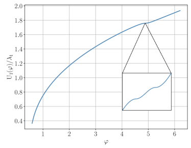
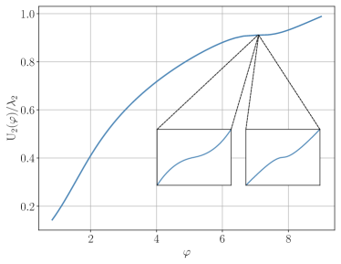
Figure 1: The potentials $\mathrm{U}_{1}(\varphi)=V_{1}(\phi)$ (left panel) $\mathrm{U}_{2}(\varphi)=V_{2}(\phi)$ (right panel) as the functions of canonical field $\varphi$.

Working in the spatially flat Friedmann-Robertson-Walker (FRW) metric, we obtain the background equations from action (1)

$$3H^{2}=\frac{1}{2}\dot{\phi}^{2}+V(\phi)+\frac{1}{2}\dot{\phi}^{2}G(\phi),$$ (10)

$$\dot{H}=-\frac{1}{2}[1+G(\phi)]\dot{\phi}^{2},$$ (11)

$$\ddot{\phi}+3H\dot{\phi}+\frac{V_{\phi}+\dot{\phi}^{2}G_{\phi}/2}{1+G(\phi)}=0,$$ (12)

where the Hubble parameter $H=\dot{a}/a$, and the dot denotes the derivative with respect to the cosmological time $t$. To the second order of comoving curvature perturbation $\zeta$, the action reads

$$S_{2}=\frac{1}{2}\int d\tau d^{3}xz^{2}\left[\left(\zeta^{\prime}\right)^{2}-(\partial\zeta)^{2}\right],$$ (13)

where $z^{2}=2a^{2}\epsilon$, and the prime stands for the derivative with respect to the conformal time ${\tau}$, where $d\tau=dt/a(t)$. The slow-roll parameters $\epsilon$ and $\eta$ are defined as

$$\epsilon=-\frac{\dot{H}}{H^{2}},\ \eta=\frac{\dot{\epsilon}}{H\epsilon}.$$ (14)

The leading order action Eq. (13) predicts a Gaussian spectrum, while non-Gaussian features, which we will discuss in Sec. III, arise from cubic action. Varying the quadratic action with respect to ${\zeta}$, we obtain the Mukhanov-Sasaki equation Mukhanov (1985); Sasaki (1986)

$$\zeta_{k}^{\prime\prime}+2\frac{z^{\prime}}{z}\zeta_{k}^{\prime}+k^{2}\zeta_{k}=0,$$ (15)

with

$$\frac{z^{\prime}}{z}=aH\left(1+\frac{\eta}{2}\right).$$ (16)

The two-point correlation function and the power spectrum are given as follows

$$\begin{split}\langle\hat{\zeta}_{\bm{k}}\hat{\zeta}_{\bm{k}^{\prime}}\rangle&=(2\pi)^{3}\delta^{3}\left(\bm{k}+\bm{k}^{\prime}\right)|\zeta_{k}|^{2}\\ &=(2\pi)^{3}\delta^{3}\left(\bm{k}+\bm{k}^{\prime}\right)P_{\zeta}\left(k\right),\end{split}$$ (17)

where the mode function $\zeta_{k}$ is the solution to Eq. (15), and $\hat{\zeta}_{\bm{k}}$ is the quantum field of the curvature perturbation that starts evolution from Bunch-Davies vacuum. The dimensionless scalar power spectrum and its spectral index are defined by

$$\Delta^{2}_{\zeta}=\frac{k^{3}}{2\pi^{2}}P_{\zeta}\left(k\right),$$ (18)

$$n_{\mathrm{s}}(k)-1=\frac{d\mathrm{ln}\Delta^{2}_{\zeta}}{d\mathrm{ln}k}.$$ (19)

With the parameter sets in Table 1, we solve the Eqs. (10)-(12) and (15) numerically. We show in Fig. 2 the evolution of the inflaton $\phi$ and the slow-roll parameter $\epsilon$ against $e$-folds $N$, and in Fig. 3 the power spectrum. In Tables. 2 and 3, we list the power index, tensor to scalar ratio, the $e$-folds $N$, the peak scales, and the amplitude of the power spectra in models M1 and M2.

Model	$n_{s}$	$r$	$N$
M1	$0.971$	$0.0426$	$69.3$
M2	$0.969$	$0.0318$	$68.7$

Table 2: The power index, tensor to scalar ratio, and the $e$-folds $N$ in M1 and M2.

Model	$k_{\mathrm{peak}}/\mathrm{Mpc}^{-1}$	$\Delta^{2}_{\zeta}(k_{\mathrm{peak}})$	$Y^{G}_{\mathrm{PBH}}$	$M/M_{\odot}$	$f_{c}/\mathrm{Hz}$	$\Delta^{\mathrm{n}}_{3}(k_{\mathrm{peak}})$	$f_{\mathrm{NL}}$	$\Delta^{\mathrm{a}}_{3}(k_{\mathrm{peak}})$
M1	$1.66\times 10^{9}$	$0.0358$	$0.003$	$1.56\times 10^{-6}$	$2.9\times 10^{-6}$	$-44.1$	$0.76$	$-31.2$
	$5.97\times 10^{12}$	$0.0333$	$0.959$	$1.24\times 10^{-13}$	$9.8\times 10^{-3}$	$-56.6$	$0.82$	$-36.2$
M2	$5.48\times 10^{8}$	$0.0360$	$0.002$	$1.51\times 10^{-5}$	$9.2\times 10^{-7}$	$-40.6$	$0.71$	$-28.9$
	$7.05\times 10^{11}$	$0.0285$	$0.012$	$7.89\times 10^{-12}$	$1.2\times 10^{-3}$	$-21.2$	$0.34$	$-17.5$

Table 3: The peak amplitude of the power spectrum, PBH DM abundance for Gaussian approximation, the 3rd cumulant $\Delta_{3}$ at peak scales, non-Gaussianity parameter $f_{\mathrm{NL}}(k_{\text{peak}},k_{\text{peak}},k_{\text{peak}})$ and the critical frequency of SIGWs for models M1 and M2. In particular, $\Delta_{3}^{\mathrm{n}}$ is the numerical result, and $\Delta_{3}^{\mathrm{a}}$ is approximation.

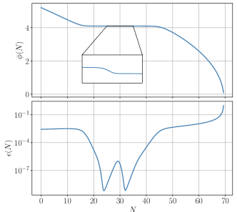
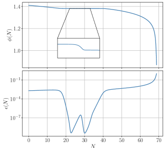
Figure 2: The evolution of inflaton $\phi$ and the slow-roll parameter $\epsilon$ with respect to $e$-folds $N,$ for models M1, the left panel, and M2, the right panel.

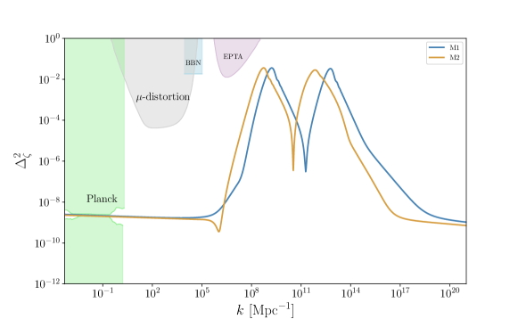
Figure 3: The power spectra produce by models M1 and M2. They are enhanced to $\mathcal{O}(0.01)$ on small scales. The shaded regions are constraints from observations Akrami et al. (2020); Inomata and Nakama (2019); Inomata et al. (2016); Fixsen et al. (1996)

.

From the upper panels of Fig. 2, there are two successive plateaus for $\phi(N)$, where the velocity of inflaton $\partial_{N}\phi$ dramatically decreases. In other words, there are two transitory phases where the inflaton behaves like in ultra slow-roll (USR) inflation Kinney (2005); Dimopoulos (2017) which correspond to the two valleys of $\epsilon(N)$ in the lower panels and lead to the double peaks in the power spectrum, as shown in Fig. 3. The second USR phase takes over before the end of the first one, which keeps $e$-folds $N$ within a reasonable range. From Fig. 3, both the power spectra produced by M1 and M2 are the order of $\mathcal{O}(10^{-9})$ at large scales, satisfying the constraints from CMB. At small scales, the power spectra are enhanced to the order of $\mathcal{O}(10^{-2})$, which serves to produce PBHs after the horizon reentry. The power spectra also satisfy the constraints from CMB $\mu$-distortion, big bang nucleosynthesis (BBN) and pulsar timing array (PTA) observations Inomata and Nakama (2019); Inomata et al. (2016); Fixsen et al. (1996).

III primordial non-Gaussianity

The inflaton in both models experiences a departure from slow roll during several $e$-folds, and the primordial non-Gaussianity may be very different from slow-roll inflation models which predict negligible non-Gaussianity. In this section, we compute the non-Gaussianity of the two models.

The bispectrum $B_{\zeta}$ is related to the three-point function as Byrnes et al. (2010); Ade et al. (2016)

$$\left\langle\hat{\zeta}_{\bm{k}_{1}}\hat{\zeta}_{\bm{k}_{2}}\hat{\zeta}_{\bm{k}_{3}}\right\rangle=(2\pi)^{3}\delta^{3}\left(\bm{k}_{1}+\bm{k}_{2}+\bm{k}_{3}\right)B_{\zeta}\left(k_{1},k_{2},k_{3}\right),$$ (20)

and the explicit lengthy expression of bispectrum $B_{\zeta}(k_{1},k_{2},k_{3})$ can be found in Refs. Hazra et al. (2013); Arroja and Tanaka (2011); Zhang et al. (2021). The non-Gaussianity parameter $f_{\text{NL}}$ is defined as Creminelli et al. (2007); Byrnes et al. (2010)

$$f_{\text{NL}}(k_{1},k_{2},k_{3})=\frac{5}{6}\frac{B_{\zeta}(k_{1},k_{2},k_{3})}{P_{\zeta}(k_{1})P_{\zeta}(k_{2})+P_{\zeta}(k_{2})P_{\zeta}(k_{3})+P_{\zeta}(k_{3})P_{\zeta}(k_{1})}.$$ (21)

We numerically compute the non-Gaussianity parameter $f_{\mathrm{NL}}$ in the squeezed limit and the equilateral limit. The results are shown in Figs. 4 and 5 for models M1 and M2, respectively. In squeezed limit, the non-Gaussianity parameter $f_{\mathrm{NL}}$ is related to the power index $n_{\mathrm{s}}-1$ by the consistency relation

$$\lim_{k_{3}\rightarrow 0}f_{\mathrm{NL}}(k_{1},k_{2},k_{3})=\frac{5}{12}(1-n_{\mathrm{s}}),\quad\text{for}~{}k_{1}=k_{2}.$$ (22)

The consistency relation was derived originally in the canonical single-field inflation with slow-roll conditions Maldacena (2003). Then it was proved to be true for any inflationary model as long as the inflaton is the only dynamical field in addition to the gravitational field during inflation Creminelli and Zaldarriaga (2004). From the upper panels in Figs. 4 and 5, we can see that the consistency relation (22) holds for the two models. Besides, the non-Gaussianity parameter $f_{\text{NL}}$ can reach as large as order $10$ at certain scales. Specifically, $\left|12f_{\mathrm{NL}}\right|/5\simeq 4$ in the squeezed limit and $\left|12f_{\mathrm{NL}}\right|/5\simeq 25$ in the equilateral limit for model M1. For model M2, $\left|12f_{\mathrm{NL}}\right|/5\simeq 5$ in the squeezed limit and $\left|12f_{\mathrm{NL}}\right|/5\simeq 10$ in the equilateral limit. For both models M1 and M2, $f_{\text{NL}}$ has a pretty large value due to the steep growth and decrease of the power spectrum. Moreover, the oscillation nature of $f_{\text{NL}}$ in both squeezed and equilateral limits originates from the small waggles in the power spectrum, as can be seen from the insets of Figs. 4 and 5.

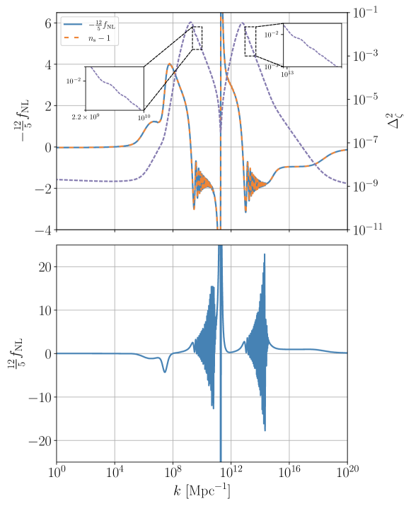
Figure 4: The primordial scalar power spectrum $\Delta^{2}_{\zeta}$ and the non-Gaussianity parameter $f_{\mathrm{NL}}$ for model M1. In the upper panel, $-\frac{12}{5}f_{\mathrm{NL}}$ in squeezed limit coincides with the spectral tilt $n_{\mathrm{s}}-1$, and the power spectrum has two peaks. We have set $k_{1}=k_{2}=10^{6}k_{3}=k$ for squeezed limit. The insets show the wiggles in $\Delta^{2}_{\zeta}$ which leads to oscillations in $f_{\mathrm{NL}}$. The lower panel shows $\frac{12}{5}f_{\mathrm{NL}}$ in the equilateral limit for the modes $k_{1}=k_{2}=k_{3}=k$.

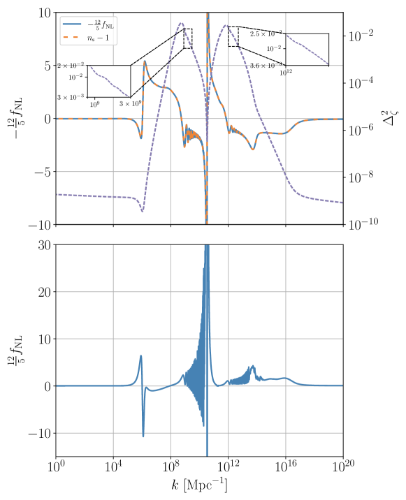
Figure 5: The primordial scalar power spectrum $\Delta^{2}_{\zeta}$ and the non-Gaussianity parameter $f_{\mathrm{NL}}$ for the model M2. In the upper panel, the power spectrum admits two peaks and the squeezed limit $-\frac{12}{5}f_{\mathrm{NL}}$ with $k_{1}=k_{2}=10^{6}k_{3}=k$ coincides the scalar spectral tilt $n_{\mathrm{s}}-1$. The insets show the wiggles in $\Delta_{\zeta}^{2}$ which leads to oscillations in $f_{\mathrm{NL}}$. The lower panel shows $\frac{12}{5}f_{\mathrm{NL}}$ in the equilateral limit.

IV PBHs

When the primordial curvature perturbation reenters the horizon during radiation dominated era, if the density contrast exceeds the threshold, it may cause gravitational collapse to form PBHs. The mass of PBH is $\gamma M_{\mathrm{hor}}$, where $M_{\mathrm{hor}}$ is the horizon mass and we choose the factor $\gamma=0.2$ Carr (1975). The current fractional energy density of PBHs with mass $M$ in DM is Carr et al. (2016); Di and Gong (2018)

$$\begin{split}Y_{\text{PBH}}(M)=&\frac{\beta(M)}{3.94\times 10^{-9}}\left(\frac{\gamma}{0.2}\right)^{1/2}\left(\frac{g_{*}}{10.75}\right)^{-1/4}\times\left(\frac{0.12}{\Omega_{\text{DM}}h^{2}}\right)\left(\frac{M}{M_{\odot}}\right)^{-1/2},\end{split}$$ (23)

where $M_{\odot}$ is the solar mass, $g_{*}$ is the effective degrees of freedom at the formation time, $\Omega_{\text{DM}}$ is the current energy density parameter of DM, and $\beta$ is the fractional energy density of PBHs at the formation.

For Gaussian statistic comoving curvature perturbation $\zeta$ Özsoy et al. (2018); Tada and Yokoyama (2019)

$$\beta^{G}(M)\approx\sqrt{\frac{2}{\pi}}\frac{\sigma_{R}(M)}{\delta_{c}}\exp\left(-\frac{\delta_{c}^{2}}{2\sigma^{2}_{R}(M)}\right),$$ (24)

where $\delta_{c}$ is the critical density contrast for the PBHs formation, and $\sigma^{2}_{R}$ is the variance of $\delta_{R}$, the density contrast $\delta$ smoothed on the horizon scales $R=1/(aH)$

$$\delta_{R}(\bm{x})=\int d^{3}y\text{W}(|\bm{x}-\bm{y}|,R)\delta(\bm{y}),$$ (25)

where W is a window function. During radiation domination, the comoving curvature perturbation is related to density contrast as Musco (2019); De Luca et al. (2019),

$$\delta(\bm{x})=\frac{4}{9}\left(\frac{1}{aH}\right)^{2}\nabla^{2}\zeta(\bm{x}).$$ (26)

Then

$$\sigma^{2}_{R}=\left(\frac{4}{9}\right)^{2}\int\frac{dk}{k}\widetilde{\text{W}}^{2}(kR)(kR)^{4}\Delta^{2}_{\zeta}(k),$$ (27)

$\widetilde{\text{W}}$ is the Fourier transform of window function. We will use a Gaussian window function $\widetilde{\mathrm{W}}(x)=\mathrm{e}^{-x^{2}/2}$. The effective degrees of freedom $g_{*}=107.5$ for $T>300$ GeV and $g_{*}=10.75$ for $0.5\text{~{}MeV}<T<300\text{~{}GeV}$. We take the observational value $\Omega_{\text{DM}}h^{2}=0.12$ Aghanim et al. (2020) and $\delta_{c}=0.4$ Harada et al. (2013); Tada and Yokoyama (2019); Escrivà et al. (2020) in the calculation of PBH abundance . The relation between the PBH mass $M$ and the scale $k$ is Di and Gong (2018)

$$M(k)=3.68\left(\frac{\gamma}{0.2}\right)\left(\frac{g_{*}}{10.75}\right)^{-1/6}\left(\frac{k}{10^{6}\ \text{Mpc}^{-1}}\right)^{-2}M_{\odot}.$$ (28)

With Eqs. (23), (24), (28) and the power spectrum obtained in section II, we compute the PBH DM abundance with Gaussian perturbation, $Y^{G}_{\mathrm{PBH}}$, the results are shown in Table 3 and Fig. 6. As excepted, there are two mass ranges of PBHs. From Fig. 6, for the mass range $M_{\mathrm{PBH}}\sim 10^{-13}-10^{-12}M_{\odot}$, the PBHs can be the dominance of DM in model M1. The PBH abundance at the peak is about $Y^{G}_{\mathrm{PBH}}\simeq 0.959$, then almost all DM is PBHs. For M2, $Y^{G}_{\mathrm{PBH}}\simeq 0.012$ is about one percent. In the mass range $M_{\mathrm{PBH}}\sim 10^{-6}-10^{-5}M_{\odot}$, the peak of $Y^{G}_{\mathrm{PBH}}$ is about $0.003$ and $0.002$ for M1 and M2, respectively. In this mass range, PBHs can be used to explain the origin of Planet 9.

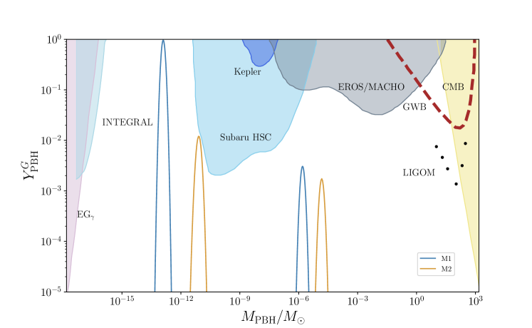
Figure 6: The PBH DM abundance $Y^{G}_{\mathrm{PBH}}$ produced by model M1 and model M2 with Gaussian statistic perturbation. The shaded regions, the dashed line and the dotted line are the constraints on PBHs abundance from various observations, please refer to Sato-Polito et al. (2019); Carr et al. (2010); Laha (2019); Dasgupta et al. (2020); Niikura et al. (2019); Griest et al. (2013); Tisserand et al. (2007); Ali-Haïmoud et al. (2017); Raidal et al. (2017); Ali-Haïmoud and Kamionkowski (2017); Poulin et al. (2017); Wang et al. (2019) and references therein for the details.

As shown in Sec. III, large non-Gaussianities are produced in M1 and M2, so it is necessary to consider the effect of non-Gaussianity on PBH abundance. The non-Gaussianity-corrected $\beta$ is related to $\beta^{G}$ from Gaussian spectrum by Franciolini et al. (2018); Kehagias et al. (2019); Atal and Germani (2019); Riccardi et al. (2021)

$$\beta=\text{e}^{\Delta_{3}}\beta^{G},$$ (29)

where $\Delta_{3}$ is called the 3rd cumulant,

$$\Delta_{3}=\frac{1}{3!}\left(\frac{\delta_{c}}{\sigma_{R}}\right)^{2}S_{3}\delta_{c},$$ (30)

and

$$S_{3}=\frac{\left\langle\delta_{R}(\bm{x})\delta_{R}(\bm{x})\delta_{R}(\bm{x})\right\rangle}{\sigma^{4}_{R}}.$$ (31)

With Gaussian window function, after some calculation, we get

$$\begin{split}\left\langle\delta_{R}(\bm{x})\delta_{R}(\bm{x})\delta_{R}(\bm{x})\right\rangle&=-64\left(\frac{4}{9}\right)^{3}\frac{2}{\left(2\pi\right)^{4}}k^{6}\\ &\quad\times\int^{\infty}_{0}du\int^{\infty}_{0}dv\int^{u+v}_{|u-v|}dwu^{3}v^{3}w^{3}\text{e}^{-u^{2}}\text{e}^{-v^{2}}\text{e}^{-w^{2}}B_{\zeta}(\sqrt{2}uk,\sqrt{2}vk,\sqrt{2}wk).\end{split}$$ (32)

Since the mass of PBHs is almost monochromatic, we can consider only the correction on peak scales. This triple integral is too complicated to perform analytically. We approximately replace $B_{\zeta}(\sqrt{2}uk,\sqrt{2}vk,\sqrt{2}wk)$ by $B_{\zeta}(\sqrt{2}k_{\mathrm{peak}},\sqrt{2}k_{\mathrm{peak}},\sqrt{2}k_{\mathrm{peak}})$ at peaks. This will be justified by numerical computation in our models.

Around the peak, the integral is approximately

$$\left\langle\delta_{R}(\bm{x})\delta_{R}(\bm{x})\delta_{R}(\bm{x})\right\rangle_{\mathrm{peak}}\simeq-\frac{800}{19683\sqrt{3}\pi^{3}}k_{\text{peak}}^{6}B_{\zeta}(\sqrt{2}k_{\text{peak}},\sqrt{2}k_{\text{peak}},\sqrt{2}k_{\text{peak}}).$$ (33)

Considering that $B_{\zeta}$ scaling as $k^{-6}$, then

$$\left\langle\delta_{R}(\bm{x})\delta_{R}(\bm{x})\delta_{R}(\bm{x})\right\rangle_{\mathrm{peak}}\simeq-\frac{1}{8}\frac{800}{19683\sqrt{3}\pi^{3}}k_{\text{peak}}^{6}B_{\zeta}(k_{\text{peak}},k_{\text{peak}},k_{\text{peak}}).$$ (34)

Substituting Eqs. (27) and (34) into (30), we get

$$\begin{split}\Delta_{3}(k_{\mathrm{peak}})&\simeq-\frac{80\sqrt{3}\pi\delta^{3}_{c}}{19683}\frac{\left(\Delta^{2}_{\zeta}(k_{\text{peak}})\right)^{2}}{\sigma^{6}_{R}}f_{\mathrm{NL}}(k_{\text{peak}},k_{\text{peak}},k_{\text{peak}})\\ &\sim-\frac{135\sqrt{3}\pi}{32}\frac{\delta^{3}_{c}}{\Delta^{2}_{\zeta}(k_{\text{peak}})}f_{\mathrm{NL}}(k_{\text{peak}},k_{\text{peak}},k_{\text{peak}})\\ &\approx-23\frac{\delta^{3}_{c}}{\Delta^{2}_{\zeta}(k_{\text{peak}})}f_{\mathrm{NL}}(k_{\text{peak}},k_{\text{peak}},k_{\text{peak}}),\end{split}$$ (35)

where we used the approximation $\sigma^{2}_{R}\sim 8\Delta^{2}_{\zeta}/81$. Note that the expression of $\Delta_{3}(k_{\mathrm{peak}})$ (35) is underestimated because $\sigma^{2}_{R}$ is actually smaller than $8\Delta^{2}_{\zeta}/81$. The effect of non-Gaussianity of curvature perturbation $\zeta$ on PBH abundance is significant unless $|\Delta_{3}(k_{\mathrm{peak}})|\lesssim 1$, namely $|f_{\mathrm{NL}}(k_{\text{peak}},k_{\text{peak}},k_{\text{peak}})|\lesssim\Delta^{2}_{\zeta}(k_{\text{peak}})/(23\delta^{3}_{c})\sim\mathcal{O}(10^{-2})$. The numerical result $\Delta^{\mathrm{n}}_{3}(k_{\mathrm{peak}})$ and approximate result $\Delta^{\mathrm{a}}_{3}(k_{\mathrm{peak}})$ given by Eq. (35) are shown in Table 3. We see that the analytic and numerical results are of the same order. The factor $\text{e}^{\Delta_{3}}$ can be extremely small as $\Delta_{3}\lesssim-10$, and thus $\beta$ is rather infinitesimal. It seems that even though the power spectrum of $\zeta$ is amplified to order $\mathcal{O}(10^{-2})$, the production of PBHs may be violently suppressed by the effect from non-Gaussianities. But honestly, enhancement is also possible as long as $\Delta_{3}>0$, that is, $f_{\mathrm{NL}}(k_{\text{peak}},k_{\text{peak}},k_{\text{peak}})<0$ for some models.

The above discussion implies that the abundance of PBH DM could be highly overestimated (or underestimated) without considering non-Gaussianity of $\zeta$. In our model, $f_{\mathrm{NL}}(k_{\text{peak}},k_{\text{peak}},k_{\text{peak}})\sim\mathcal{O}(1)$, which leads to a suppression of PBH formation.

V SIGWs

In Sec. II, we got the power spectrum enhanced at small scales, and we expect that the SIGWs are also amplified. In this section, we compute the energy density fraction of SIGWs.

In Newtonian gauge, the perturbed metric is

$$ds^{2}=a^{2}(\tau)\left[-(1+2\Phi)d\tau^{2}+\left\{(1-2\Phi)\delta_{ij}+\frac{1}{2}h_{ij}\right\}dx^{i}x^{j}\right],$$ (36)

where ${\Phi}$ is the Bardeen potential, and the second-order tensor perturbation ${h_{ij}}$ is transverse and traceless, ${\partial_{i}h_{ij}=h_{ii}=0}$. In Fourier space, the tensor perturbation is

$$h_{ij}\left(\bm{x},\tau\right)=\int\frac{d^{3}\bm{k}}{\left(2\pi\right)^{3/2}}\text{e}^{i\bm{k}\cdot\bm{x}}\left[h^{+}_{\bm{k}}\left(\tau\right)e^{+}_{ij}\left(\bm{k}\right)+h^{\times}_{\bm{k}}\left(\tau\right)e^{\times}_{ij}\left(\bm{k}\right)\right],$$ (37)

where the polarization tensors ${e^{+}_{ij}\left(\bm{k}\right)}$ and ${e^{\times}_{ij}\left(\bm{k}\right)}$ are

$$\begin{split}&e^{+}_{ij}\left(\bm{k}\right)=\frac{1}{\sqrt{2}}\left[e_{i}\left(\bm{k}\right)e_{j}\left(\bm{k}\right)-\overline{e}_{i}\left(\bm{k}\right)\overline{e}_{j}\left(\bm{k}\right)\right],\\ &e^{\times}_{ij}\left(\bm{k}\right)=\frac{1}{\sqrt{2}}\left[e_{i}\left(\bm{k}\right)\overline{e}_{j}\left(\bm{k}\right)+\overline{e}_{i}\left(\bm{k}\right)e_{j}\left(\bm{k}\right)\right],\end{split}$$ (38)

with ${e_{i}\left(\bm{k}\right)}$ and ${\overline{e}_{i}\left(\bm{k}\right)}$ are two orthonormal basis vectors which are orthogonal to the wave vector ${\bm{k}}$. Neglecting the anisotropic stress, the equation of motion for the tensor perturbation $h_{\bm{k}}$ of either polarization is

$$h^{{}^{\prime\prime}}_{\bm{k}}\left(\tau\right)+2\mathcal{H}h^{{}^{\prime}}_{\bm{k}}\left(\tau\right)+k^{2}h_{\bm{k}}\left(\tau\right)=4S_{\bm{k}}\left(\tau\right),$$ (39)

where ${\mathcal{H}=a^{\prime}/a}$ and $S_{\bm{k}}\left(\tau\right)$ is

$$S_{\bm{k}}\left(\tau\right)=\int\frac{d^{3}\tilde{\bm{k}}}{\left(2\pi\right)^{3/2}}e^{ij}\left(\bm{k}\right)\tilde{k}_{i}\tilde{k}_{j}f(\bm{k},\tilde{\bm{k}},\tau)\phi_{\tilde{\bm{k}}}\phi_{\bm{k}-\tilde{\bm{k}}},$$ (40)

in which

$$\begin{split}f(\bm{k},\tilde{\bm{k}},\tau)=&2T_{\phi}(\tilde{k}\tau)T_{\phi}(|\bm{k}-\tilde{\bm{k}}|\tau)\\ &+\frac{4}{3\left(1+w\right)\mathcal{H}^{2}}\left(T^{\prime}_{\phi}(\tilde{k}\tau)+\mathcal{H}T_{\phi}(\tilde{k}\tau)\right)\left(T^{\prime}_{\phi}(|\bm{k}-\tilde{\bm{k}}|\tau)+\mathcal{H}T_{\phi}(|\bm{k}-\tilde{\bm{k}}|\tau)\right),\end{split}$$ (41)

The transfer function $T_{\phi}$ for the Bardeen potential $\Phi$ is defined with its primordial value $\phi_{\bm{k}}$ as

$$\Phi_{\bm{k}}\left(\tau\right)=\phi_{\bm{k}}T_{\phi}\left(k\tau\right).$$ (42)

The primordial value ${\phi_{\bm{k}}}$ is related to the comoving curvature perturbation as

$$\langle\phi_{\bm{k}}\phi_{\bm{p}}\rangle=\delta^{3}\left(\bm{k}+\bm{p}\right)\frac{2\pi^{2}}{k^{3}}\left(\frac{3+3w}{5+3w}\right)^{2}\mathcal{P}_{\zeta}\left(k\right),$$ (43)

here $\mathcal{P}_{\zeta}$ is defined by

$$\begin{split}\langle\hat{\zeta}_{\bm{k}}\hat{\zeta}_{\bm{k}^{\prime}}\rangle&=(2\pi)^{3}\delta^{3}\left(\bm{k}+\bm{k}^{\prime}\right)|\zeta_{k}|^{2}\\ &=(2\pi)^{3}\delta^{3}\left(\bm{k}+\bm{k}^{\prime}\right)\frac{2\pi^{2}}{k^{3}}\mathcal{P}_{\zeta}\left(k\right).\end{split}$$ (44)

It is worth mentioning that we do not assume anything about the statistical nature of the primordial curvature perturbation, so $\mathcal{P}_{\zeta}$ is affected by the self-interactions of $\zeta$, in which the leading is the primordial non-Gaussianity, and there will be the difference between $\mathcal{P}_{\zeta}$ and $\Delta^{2}_{\zeta}$ obtained in Sec. II.

The solution to Eq. (39) is given by the Green function

$$h_{\bm{k}}\left(\tau\right)=\frac{4}{a\left(\tau\right)}\int^{\tau}d\overline{\tau}G_{k}\left(\tau,\overline{\tau}\right)a\left(\overline{\tau}\right)S_{\bm{k}}\left(\overline{\tau}\right),$$ (45)

where the Green’s function satisfies the equation

$$G^{{}^{\prime\prime}}_{\bm{k}}(\tau,\overline{\tau})+\left(k^{2}-\frac{a^{{}^{\prime\prime}}\left(\tau\right)}{a\left(\tau\right)}\right)G_{\bm{k}}\left(\tau,\overline{\tau}\right)=\delta\left(\tau-\overline{\tau}\right).$$ (46)

During radiation domination, ${w=1/3}$, the Green’s function is

$$G_{\bm{k}}\left(\tau,\overline{\tau}\right)=\frac{\sin\left[k\left(\tau-\overline{\tau}\right)\right]}{k},$$ (47)

and the transfer function is

$$T_{\phi}\left(x\right)=\frac{9}{x^{2}}\left(\frac{\sin\left(x/\sqrt{3}\right)}{x/\sqrt{3}}-\cos\left(x/\sqrt{3}\right)\right),$$ (48)

where ${x=k\tau}$. The power spectrum of tensor perturbation is defined in a similar way to $\mathcal{P}_{\zeta}$ as

$$\langle h_{\bm{k}}\left(\tau\right)h_{\bm{p}}\left(\tau\right)\rangle=\delta^{3}\left(\bm{k}+\bm{p}\right)\frac{2\pi^{2}}{k^{3}}\mathcal{P}_{h}\left(k,\tau\right).$$ (49)

Combing the Eqs. (40), (45) and (49), we get the semianalytic expression for $\mathcal{P}_{h}$ Kohri and Terada (2018); Espinosa et al. (2018b)

$$\mathcal{P}_{h}\left(k,\tau\right)=4\int^{\infty}_{0}dv\int^{1+v}_{\left|1-v\right|}du\left(\frac{4v^{2}-\left(1+v^{2}-u^{2}\right)^{2}}{4vu}\right)^{2}I^{2}_{RD}\left(u,v,x\right)\mathcal{P}_{\zeta}\left(vk\right)\mathcal{P}_{\zeta}\left(uk\right),$$ (50)

where ${u=|\bm{k}-\tilde{\bm{k}}|/k,v=\tilde{|\bm{k}|}/k}$. At late time, ${k\tau\gg 1\Leftrightarrow x\rightarrow\infty}$, the time average of ${I^{2}_{\mathrm{RD}}\left(u,v,x\rightarrow\infty\right)}$ is

$$\begin{split}\overline{I_{\mathrm{RD}}^{2}(v,u,x\rightarrow\infty)}=&\frac{1}{2x^{2}}\left(\frac{3(u^{2}+v^{2}-3)}{4u^{3}v^{3}}\right)^{2}\left\{\left(-4uv+(u^{2}+v^{2}-3)\log\left|\frac{3-(u+v)^{2}}{3-(u-v)^{2}}\right|\right)^{2}\right.\\ &\left.\vphantom{\log\left|\frac{3-(u+v)^{2}}{3-(u-v)^{2}}\right|^{2}}\qquad\qquad\qquad\qquad\qquad+\pi^{2}(u^{2}+v^{2}-3)^{2}\Theta\left(v+u-\sqrt{3}\right)\right\}.\end{split}$$ (51)

The energy density parameter of SIGWs per logarithmic interval of ${k}$ is

$$\Omega_{\mathrm{GW}}\left(k\right)=\frac{1}{24}\left(\frac{k}{\mathcal{H\left(\tau\right)}}\right)^{2}\overline{\mathcal{P}_{h}\left(k,\tau\right)}.$$ (52)

Notice that at late time, $\Omega_{\mathrm{GW}}$ is a constant since GWs behave like free radiation. With this featrue, we can also express the fractional energy density of SIGWs today $\Omega_{\mathrm{GW},0}$ as Espinosa et al. (2018b)

$$\Omega_{\mathrm{GW},0}\left(k\right)=\Omega_{\mathrm{GW}}\left(k\right)\frac{\Omega_{r,0}}{\Omega_{r}\left(\tau\right)},$$ (53)

where we choose $\Omega_{r}=1$ because we are considering the radiation domination.

As mentioned above, the perturbations that induce SIGWs can be non-Gaussian, in order to estimate the contribution of non-Gaussianity to SIGWs, using the nonlinear coupling constant $f_{\text{NL}}$ defined as Verde et al. (2000); Komatsu and Spergel (2001)

$$\zeta(\bm{x})=\zeta^{G}(\bm{x})+\frac{3}{5}f_{\text{NL}}(\zeta^{G}(\bm{x})^{2}-\langle\zeta^{G}(\bm{x})^{2}\rangle),$$ (54)

where $\zeta^{G}$ is the linear Gaussian part of the curvature perturbation. Then the power spectrum of $\zeta$ taking into account of the non-Gaussianity can be expressed as

$$\mathcal{P}_{\zeta}(k)=\mathcal{P}^{G}_{\zeta}(k)+\mathcal{P}^{NG}_{\zeta}(k),$$ (55)

where $\mathcal{P}^{G}_{\zeta}(k)=\Delta^{2}_{\zeta}(k)$, and

$$\mathcal{P}^{NG}_{\zeta}(k)=\left(\frac{3}{5}\right)^{2}\frac{k^{3}}{2\pi}f^{2}_{\mathrm{NL}}\int d^{3}\bm{p}\frac{\mathcal{P}^{G}_{\zeta}(p)}{p^{3}}\frac{\mathcal{P}^{G}_{\zeta}(|\bm{k}-\bm{p}|)}{|\bm{k}-\bm{p}|^{3}}.$$ (56)

It was shown that the non-Gaussian contribution to SIGWs exceeds the Gaussian part if $\left(\frac{3}{5}\right)^{2}f^{2}_{\text{NL}}\mathcal{P}^{G}_{\zeta}\gtrsim 1$ Cai et al. (2019a). Taking $f_{\mathrm{NL}}$ as the estimator to parameterize the magnitude of non-Gaussianity Chen et al. (2007), we find the contribution from the non-Gaussian curvature perturbations to SIGWs is negligible, because $f_{\text{NL}}\sim\mathcal{O}(1)$ is not very large at the peak where power spectrum $\mathcal{P}^{G}_{\zeta}$ culminates, as shown in Figs. 4 and 5. In the following, we safely use $\Delta^{2}_{\zeta}$ we get in Sec. II instead of $\mathcal{P}_{\zeta}$ to compute SIGWs.

We compute the $\Omega_{\mathrm{GW}}$ and the results are shown in Table 3 and Fig. 7. As expected, there are also double peaks in SIGWs at the corresponding scales, and both the peaks are observable in the future. The milli-Hertz SIGWs can be tested by TianQin, Taiji, and LISA. The $10^{-6}$ Hz SIGWs leave a blue-tilted spectrum on the SKA region.

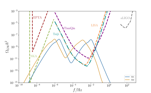
Figure 7: The SIGWs generate by model M1 and model M2. The fuchsia dashed curve denotes the EPTA limit Ferdman et al. (2010); Hobbs et al. (2010); McLaughlin (2013); Hobbs (2013) , the lime dashed curve denotes the SKA limit Moore et al. (2015), the purple dashed curve in the middle denotes the TianQin limit Luo et al. (2016), the dark cyan dotted-dashed curve shows the Taiji limit Hu and Wu (2017), the orange dashed curve shows the LISA limit Amaro-Seoane et al. (2017), and the gray dashed curve denotes the aLIGO limit Harry (2010); Aasi et al. (2015).

VI conclusion

For PBHs to be all (or most of) the DM, the violation of slow-roll conditions in single-field inflation is necessary as the slow-roll inflation predicts nearly scale-invariant power spectrum of order $\mathcal{O}(10^{-9})$ which hardly generates a significant abundance of PBHs and observable SIGWs. On the other hand, the violation of slow-roll conditions may lead to considerable primordial non-Gaussianity of curvature perturbation. We find that the abundance of PBHs is sensitive to the primordial non-Gaussianity of curvature perturbation and will be altered significantly if the non-Gaussianity parameter $|f_{\mathrm{NL}}(k_{\text{peak}},k_{\text{peak}},k_{\text{peak}})|\gtrsim\Delta^{2}_{\zeta}(k_{\mathrm{peak}})/(23\delta^{3}_{c})\sim\mathcal{O}(10^{-2})$. Whether the PBH abundance is suppressed or enhanced depends on $f_{\mathrm{NL}}(k_{\text{peak}},k_{\text{peak}},k_{\text{peak}})$ being positive or negative, respectively.

We propose a noncanonical inflation model with a double-peak coupling function in the noncanonical kinetic term, which is equivalent to a canonical model with double quasi-inflection points in the potential by field-redefinition. The model driven by both $\lambda\phi^{2/5}$ potential and Higgs potential can amplify the power spectrum to $\mathcal{O}(10^{-2})$ at two different small scales while satisfying the constraints from CMB at large scales and keeping $e$-folds $N\sim 69$. We also numerically calculate the primordial non-Gaussianity in squeezed and equilateral limits. We find that the consistency relation is valid even when the slow-roll conditions are violated. Regrettably, our model predicts large non-Gaussianity with $f_{\mathrm{NL}}(k_{\text{peak}},k_{\text{peak}},k_{\text{peak}})\sim\mathcal{O}(1)$ that is positive and the PBH abundance is suppressed saliently, even though the power spectrum is about $\mathcal{O}(0.01)$. However, the energy density of SIGWs is insensitive to primordial non-Gaussianity and thus observable. In this regard, SIGWs are better at characterizing the small-scale power spectrum. In our models, SIGWs will leave a blue-tilted spectrum in SKA sensitivity, and a peak in the sensitivities of LISA, Taiji and TianQin. In addition, it is possible that we observe SIGWs in SGWB, but PBHs hardly exist in the corresponding mass ranges, taking into account the primordial non-Gaussianity.