The Simplest Viscous Flow

Abstract

We illustrate an atomistic periodic two-dimensional stationary shear flow, $u_{x}=\langle\ \dot{x}\ \rangle=\dot{\epsilon}y$, using the simplest possible example, the periodic shear of just two particles ! We use a short-ranged “realistic” pair potential, $\phi(r<2)=(2-r)^{6}-2(2-r)^{3}$. Many body simulations with it are capable of modelling the gas, liquid, and solid states of matter. A useful mechanics generating steady shear follows from a special (“Kewpie-Doll” $\sim$ “$qp$-Doll”) Hamiltonian based on the Hamiltonian coordinates $\{q\}$ and momenta $\{p\}$ : ${\cal H}(q,p)\equiv K(p)+\Phi(q)+\dot{\epsilon}\sum qp$. Choosing $qp\rightarrow yp_{x}$ the resulting motion equations are consistent with steadily shearing periodic boundaries with a strain rate $(du_{x}/dy)=\dot{\epsilon}$. The occasional $x$ coordinate jumps associated with periodic boundary crossings in the $y$ direction provide a Hamiltonian that is a piecewise-continuous function of time. A time-periodic isothermal steady state results when the Hamiltonian motion equations are augmented with a continuously variable thermostat generalizing Shuichi Nosé’s revolutionary ideas from 1984. The resulting distributions of coordinates and momenta are interesting multifractals, with surprising irreversible consequences from strictly time-reversible motion equations.

I Introduction to Isothermal Molecular Dynamics

Molecular Dynamics began in the 1950s with Fermi, Pasta, and Ulam’s investigation of one-dimensional anharmonic chains. That work was soon followed with Alder and Wainwright’s dynamical exploration of the pressure/volume equations of state for two-dimensional hard disks and three-dimensional hard spheres. While Fermi was surprised that his chains never reached equilibrium, Alder and Wainwright found that disks and spheres equilibrated rapidly, in just a few collision times. Alder and Wainwright also produced evidence for first-order melting/freezing transitions for hard particles. These earliest molecular dynamics simulations used from dozens to hundreds of particles, solving Newton’s motion equations. By 2008 quadrillion-atom molecular dynamics $(N=10^{12})$ was feasibleb1 . Germann and Kadau found that a single timestep, for a short-ranged pair potential in an unstable cubic lattice and with $N=10^{4}\times 10^{4}\times 10^{4}$ particles, took about a minute of computer time to execute.

Periodic boundary conditions are the simplest choice, with any particle exiting at a system boundary simultaneously introduced on the opposite side. In the absence of phase transitions such homogeneous 100-particle simulations are sufficient to determine the mechanical pressure/volume and thermal energy/temperature equations of state with accuracies of order 1%.

Nonequilibrium simulations require more sophisticated boundary conditions. In his 1974 thesis work at Livermore Ashurst sandwiched rectangular Newtonian manybody systems between two “fluid-wall” regions.b2 The particles in these bounding walls had specified values of the mean velocity and the mean-squared velocity imposed at every timestep. With different boundary velocities the resulting shear viscosity could be measured. With different boundary kinetic temperatures, $K/N\sim T\sim\langle\ (p^{2})\ \rangle$, heat flow could be simulated and the thermal conductivity measured. By 1980 it was well accepted that the equilibrium and nonequilibrium properties for manybody systems provided excellent models for the behavior of real fluids, both at, and away from, equilibrium.

In 1984 Shuichi Nosé formulated a temperature-dependent Hamiltonian reproducing Gibbs’ canonical-ensemble distribution of energies, $\propto\exp[-E/kT]$. His formulationb3 ; b4 included a relaxation time $\tau$ with rapid relaxation consistent with Ashurst’s rescaling of the mean-squared velocity to impose temperatures within the fluid walls. The “Nosé-Hoover” version of this workb5 is better suited to computation than was Nosé’s original Hamiltonian-based algorithm. For $N$ particles of unit mass in $D$ space dimensions the equations of motion have the form:

$$\dot{q}=p\ ;\ \dot{p}=F(q)-\zeta p\ ;\ \dot{\zeta}=[\ (\sum p^{2}/NDkT)-1\ ]/\tau^{2}\ .$$

For $D=2$ $q$ and $p$ have both $x$ and $y$ components: $q=(x,y)\ ;\ p=(p_{x},p_{y})$. $k$ is Boltzmann’s constant (for convenience chosen equal to unity) and $T$ is the specified kinetic temperature, $\langle\ p^{2}/2k\ \rangle=\langle\ p^{2}/2\ \rangle.$

The “friction coefficient” $\zeta$ imposes integral control on the kinetic temperature in a time of order $\tau$. In the instantaneous limit, $\tau\rightarrow 0$, integral control corresponds to Ashurst’s velocity rescaling. In the equilibrium case, without external driving, Hoover pointed out that the time-averaged distribution of the friction coefficient $\zeta$ is Gaussian, with zero mean. We will see that this changes away from equilibrium where $\langle\ \zeta\ \rangle$ corresponds to entropy production, and is necessarily positive.

II Imposing Shear on Molecular Dynamics with Doll’s Tensor

With controlled boundary conditions molecular dynamics can be generalized to nonequilibrium flows characterized by viscosity and thermal conductivity. These material properties characterize the response of fluids or solids to gradients in the velocity or the temperature. Viscosity is the simpler of these possibilities. Periodic boundary conditions are natural for shear deformation.

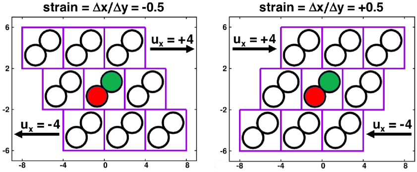
Figure 1: Steady time-dependent shearing boundary conditions are illustrated here for unit strainrate $(du_{x}/dy)=1$ with a periodic $4\times 4$ cell containing Particles 1 and 2. The three upper images of the central cell move to the right at $u_{x}=+4$ while the three lower images move left with $u_{x}=-4$. Particles 1 and 2 (red and green) occupy the central cell with a fixed center of mass at the origin. The force on Particle 1 comes directly from Particle 2 or its nearest image (from the eight neighboring cells) and is nonzero whenever that separation is less than the range of the forces, $r_{12}<2$. The force on Particle 2 is equal in magnitude and opposite in sign, maintaining the center-of-mass position at the origin, the center of the central cell. Whenever a horizontal cell boundary is crossed the systematic horizontal velocity component $\dot{x}$ changes by $\pm 4$ and the $x$ coordinate undergoes a change equal to the fractional part of the strain, $\dot{\epsilon}t-[\dot{\epsilon}t]_{\rm integer}$, where $t$ is the time. The crossing of a vertical cell boundary changes only the value of the $x$ coordinate, by $\pm 4$, just as in the usual application of periodic boundary conditions. To avoid the unnecessary loss of significant figures whenever the strain reaches $+0.5$, as shown at the right, the strain is decreased by unity to $-0.5$, the strain shown at the left.

A straightforward viscous modification of equilibrium molecular dynamics can be implemented by imparting a systematic motion to the neighbors of a periodically-repeated simulation, as illustrated in Figure 1. The figure shows the details of two particles interacting periodically. Three parallel periodic rows, of $3N=6$ particles each are required. There is a systematic boundary motion in the $x$ direction which increases linearly with $y$. The “Doll’s Tensor” Hamiltonian (named after the $qp$ term reminiscent of the Kewpie Doll) consistent with this motion was introduced by Hoover in 1980b6 . With $(qp)\rightarrow(yp_{x})$ this Hamiltonian is

$${\cal H}_{\rm Doll^{\prime}s}=\sum(p^{2}/2)+\Phi+\dot{\epsilon}\sum yp_{x}\rightarrow\{\ \dot{x}=+(\partial{\cal H}/\partial p_{x})=p_{x}+\dot{\epsilon}y\ \}\ .$$

The new term proportional to the strain rate, $\dot{\epsilon}=(du_{x}/dy)$, along with periodic boundaries in the $x$ and $y$ directions, generates a shear flow. With just two particles, such a model provides the simplest atomistic simulation of viscous shear flow. The Doll’s Tensor equations of motion, applied to momenta $(p_{x},p_{y})$, with vanishing sums, produce a systematic increase of $x$ velocity with $y$, $\dot{\epsilon}y$:

$$\{\ \dot{x}=p_{x}+\dot{\epsilon}y\ ;\ \dot{y}=p_{y}\ ;\ \dot{p}_{x}=F_{x}\ ;\ \dot{p}_{y}=F_{y}-\dot{\epsilon}p_{x}\ \}\ .$$

For simplicity we consider forces $\{\ F_{x},F_{y}\ \}$ derived from a pair potential $\phi(r)$: $F(r)=-\nabla\phi(r)$. In this case the total potential is a simple sum over all pairs of particles, $\Phi=\sum\phi_{i<j}$.

With pair forces the change in the “internal” energy $E=\sum(p^{2}/2)+\Phi$ is precisely consistent with the first-law thermodynamic relation for energy conservation in the absence of heat flow, $\Delta{\rm Heat}=0\longrightarrow\Delta E=\Delta{\rm Heat}-\Delta{\rm Work}=-\Delta{\rm Work}$:

$$\dot{E}=-\dot{\epsilon}\sum^{N}(p_{x}p_{y})-\dot{\epsilon}\sum^{\rm pairs}(Fxy/r)_{i<j}=-\dot{\epsilon}P_{xy}V\ .$$

Here the force-dependent pair sum includes the particle separations in the $x$ and $y$ directions:

$$(xy/r)\equiv(x_{i}-x_{j})(y_{i}-y_{j})/\sqrt{[(x_{i}-x_{j})^{2}+(y_{i}-y_{j})^{2}]}\ .$$

Notice particularly that the First Law of Thermodynamics just given is perfectly time-reversible. In a reversed process $\dot{E}$ necessarily changes sign, as does the strain-rate $\dot{\epsilon}$. The shear component of the pressure tensor does not change with the direction of time, thus violating the empirical experience that shearing a viscous fluid requires work, whether the shearing is clockwise or counterclockwise. It is definitely paradoxical that the time-reversible laws of microscopic mechanics provide simulations obeying the Second Law, that work can be converted to heat, but not vice versa. We will extend this paradox, already present in Hamiltonian mechanics, to a nonequilibrium mechanics in which both heat and work enter, and with the same paradoxical disagreement with the Second Law.

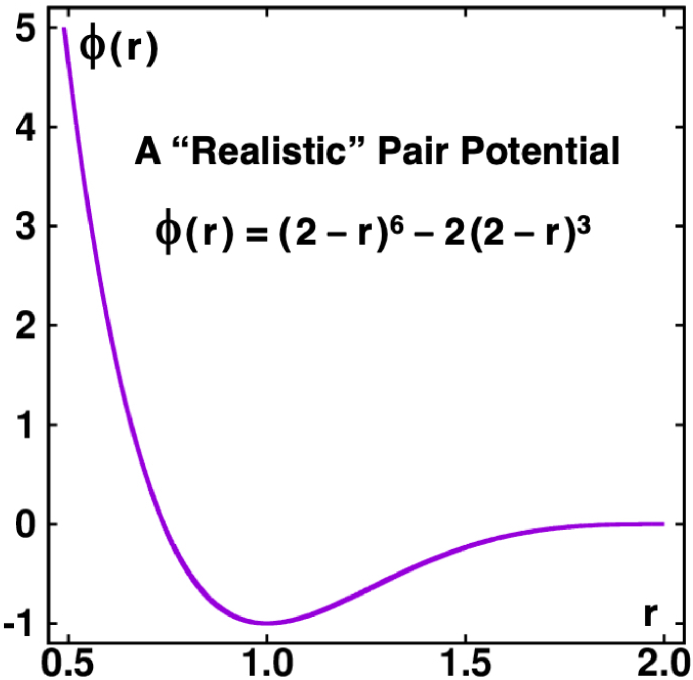
Figure 2: Pair potential for molecular dynamics simulation of shear, $\phi(r)=(2-r)^{6}-2(2-r)^{3}$. The minimum at $r=1$ sets the energy scale and the distance scale. The vanishing of both the force and its first derivative at $r=2$ provides highly-accurate Runge-Kutta trajectories.

We adopt a particularly simple pair potential, with a range $r<2$, and sufficiently realistic to generate gas, liquid, and solid phasesb7 . See Figure 2 for a plot. This pair potential function is a simple polynomial in $r$, with an attractive minimum of unity at a separation of unity, $\phi(r=1)=-1$:

$$\phi_{3}^{L}(r)=(2-r)^{6}-2(2-r)^{3}\rightarrow F=6[(2-r)^{5}-(2-r)^{2}]\ .$$

Thus the potential minimum sets both the length and the energy scales. Both the force and its first derivative vanish at the cutoff radius $r=2$, optimizing the numerical accuracy of computer simulations.

The simplest viscous flow, illustrated in Figure 1, is a two-particle dynamical system. With a potential range of 2 a periodic $4\times 4$ box is the smallest for which the interaction of the two particles involves just one of the 9 possibilities illustrated in the figure. With vanishing center-of-mass velocity the two-particle problem is equivalent to a one-particle one, with the boundary conditions including the steady motion of cells containing image particles. In the two-particle version the four time-dependent variables $(x,y,p_{x},p_{y})$ for Particle 2 exactly equal the negatives of the same variable set for Particle 1.

Let us turn next to the integration details. We like to avoid the need for developing special integration algorithms for the various types of problems described by atomistic simulations. For simplicity and accuracy we prefer fourth-order Runge-Kutta integration for all those problems that are describable with first-order differential equationsb8 . These included models in which constraints on the momentum or temperature or stress are imposed by Hamiltonian or nonHamiltonian constraints. Let us review our favorite Runge-Kutta integrator by applying it to two instructive problems. The first is the simple harmonic oscillator. This problem is useful for code development as the Runge-Kutta algorithm has an explicit analytic solution for the oscillator.

We introduce additional complexity and nonlinearity in our second pedagogical example, the periodic dynamics of two two-dimensional particles using the realistic pair potential just described, a finite-ranged very smooth polynomial in the separation. The boundaries for that problem simplify in the absence of the systematic velocity gradient of Figure 1. The static-boundary problem appears to be chaotic and might even be ergodic despite its simplicity. The problem’s description can be reduced from eight dimensions to just three by taking the constancy of the center of mass, its motion, and the conserved total energy into account. Three dimensions is just sufficient for chaos. Let us consider the details of the Runge-Kutta integration algorithm and its applications to the harmonic oscillator and the two-dimensional periodic two-body problem next.

III Two Problems Illustrating the Runge-Kutta Algorithm

III.1 The Fourth-Order Runge-Kutta Integration Algorithm

For completeness we review the programming necessary to implement the fourth-order Runge-Kutta integrator. The simplicity and accuracy of this integrator make it our first choice whenever possible. Consider solving $N$ first-order differential equations using the Runge-Kutta algorithm.

A main program calls the fourth-order Runge-Kutta subroutine to execute each timestep, advancing the $N$, ${\tt N}$ in the subroutine, time-dependent variables, stored in the vector ${\tt YNOW}$. In the subroutine, given below, the righthandsides of the $N$ first-order differential equations are evaluated successively for four different vectors, providing an averaged time derivative which is accurate through the fourth power of the timestep $dt$, DT in the program. As the timestep is specified at the beginning of each step, it can be changed “on the fly”, if necessary. For instance, a useful diagnostic for accuracy is the difference between the result of a single step $dt$ and that of two successive steps half as large, $dt/2$. If the difference is too large the step DT can be reduced to ${\tt DT/2}$. If the difference is too small ${\tt DT}$ can be doubled. The fourth-order Runge-Kutta algorithm is called at each timestep and has the effect of converting the $N$-dimensional solution vector YNOW(T) at time $t$ to its value at time $t+dt$: ${\tt YNOW(T)}\rightarrow{\tt YNOW(T+DT)}$.

  CALL RHS(YNOW,YDOT)
  DO 1 J = 1,N
1 D1(J) = YDOT(J)
  DO 2 J = 1,N
2 YNEW(J) = YNOW(J) + DT*D1(J)/2
  CALL RHS(YNEW,YDOT)
  DO 3 J = 1,N
3 D2(J) = YDOT(J)
  DO 4 J = 1,N
4 YNEW(J) = YNOW(J) + DT*D2(J)/2
  CALL RHS(YNEW,YDOT)
  DO 5 J = 1,N
5 D3(J) = YDOT(J)
  DO 6 J = 1,N
6 YNEW(J) = YNOW(J) + DT*D3(J)
  CALL RHS(YNEW,YDOT)
  DO 7 J = 1,N
7 D4(J) = YDOT(J)
  DO 8 J = 1,N
8 YNOW(J) = YNOW(J) + DT*(D1(J)+2*(D2(J)+D3(J))+D4(J))/6

III.2 Hamiltonian Dynamics of the Harmonic Oscillator

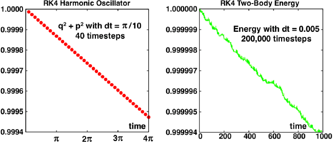
Figure 3: At the left we see the steady growth of energy error for the harmonic oscillator, with initial conditions $(q,p)=(1,0)$, shown for forty time steps of $\pi/10$. The decay of the energy is accurately linear in time with the error varying as $dt^{5}$ at a fixed time. The analytic solution to this problem is given in Wm. G. Hoover’s 1991 Elsevier book, Computational Statistical Mechanics. At the right we see the analogous error growth for the Hamiltonian dynamics of two two-dimensional particles with periodic boundary conditions for 200,000 steps of 0.005 each. Though there are collisional fluctuations the growth rate is still roughly linear and varies likewise as $dt^{5}$.

The simplest instructive application of the Runge-Kutta integrator is the harmonic oscillator example. Only two motion equations are involved, $\dot{q}=+p$ and $\dot{p}=-q$. With $(q,p)$ initially $(+1,0)$ the analytic solution has a period of $2\pi$: $q=\cos(t)\ ;\ p=-\sin(t)$. Dividing the interval $0<t<2\pi$ into 100 steps with initial values YNOW(1) = 1, YNOW(2) = 0 gives a double-precision estimate of the algorithm’s accuracy. The error in $q^{2}+p^{2}$ at $t=2\pi$ (twice the final total oscillator energy) is $8.5415\times 10^{-8}$. The history of the decrease is accurately linear in time, as is illustrated in Figure 3. Reducing the timestep twofold gives an error nearly 32 times smaller, $2.6702\times 10^{-9}$. The error ratio, 31.99, confirms that the energy error varies as $dt^{5}$, one order better than the larger seperate errors in the coordinate and momentum.

Notice that the input vector YNOW is incremented by the mean value of four estimated RHS vectors in each Runge-Kutta iteration. The derivatives D1, D2, D3, D4 are evaluated at the initial point and three subsequent nearby points. When the righthandsides of the differential equations are explicitly time-dependent, as in periodic shear, the four successive evaluations of the righthandsides in each timestep are evaluated at times T for D1, T + DT/2 for D2 and D3, and finally, T + DT for D4.

The fourth-order Runge-Kutta solution of the oscillator equations $\dot{q}=p$ and $\dot{p}=-q$ with $[q,p]$ initially $[+1,0]$, has a relatively simple and useful analytic form:

$$[q_{n},p_{n}]=[1-(dt^{6}/72)+(dt^{8}/576)]^{n/2}[+\cos(n\lambda),-\sin(n\lambda)]\ {\rm with}$$

$$\lambda\equiv\arctan\frac{[dt-(dt^{3}/6)]}{[1-(dt^{2}/2)+(dt^{4}/24)]}\ .$$

For sufficiently large $dt$, so that $dt^{8}/576$ is properly represented, this result provides a useful and informative programming check for the implementation of the Runge-Kutta integration algorithm. We can see that $(q^{2}+p^{2})$, rather than being constant at long times $ndt$, decreases as $ndt^{6}/72=tdt^{5}/72$, one order of $dt$ better than would be expected for a fourth-order method. Although the oscillator amplitude is fifth-order, both the coordinate and the momentum $[q,p]$ do exhibit errors of order $tdt^{4}$. Further analysis shows that this difference in orders is due to a “phase error” with the oscillator slowed to fourth order in $dt$, rather than reduced in amplitude. Thus the dominant error at a fixed time is a negative phase error of order $tdt^{4}$. With twenty timesteps per period a double-precision comparison of the numerical and analytical results from Runge-Kutta up to a time $2\pi$ gives agreement to a dozen significant figures.

With this interesting oscillator task successfully completed, confirming the utility and accuracy of the algorithm, fully-fledged nonlinear simulations with realistic interparticle interactions as well as both static and dynamic boundary conditions on the coordinates provide the next steps toward our goal of simulating “The simplest viscous flow”.

III.3 Equilibrium Dynamics with a Realistic Potential

The equilibrium Runge-Kutta integration of two-body dynamics with static periodic boundaries and with interparticle forces, $F(r<2)=-(d\phi/dr)=6(2-r)^{5}-6(2-r)^{2}$, is an excellent computational next step. Conservation of the energy, $E=\Phi+K=\phi_{12}+(p_{1}^{2}+p_{2}^{2})/2$ is a (nearly) foolproof check on the programming. To apply fourth-order Runge-Kutta integration the eight time-dependent variables are stored in an eight-dimensional $yy$ vector. For the coordinates we choose

$$yy(1)=x_{1}\ ;\ yy(2)=x_{2}\ ;\ yy(3)=y_{1}\ ;\ yy(4)=y_{2}$$

and for the momenta

$$yy(5)=p_{x_{1}}\ ;\ yy(6)=p_{x_{2}}\ ;\ yy(7)=p_{y_{1}}\ ;\ yy(8)=p_{y_{2}}\ .$$

The $x$ coordinates are confined to the $4\times 4$ periodic box, both initially and after every integration step, with four statements

if(x1.lt.-2) yy(1) = yy(1) + 4
if(x1.gt.+2) yy(1) = yy(1) - 4
if(x2.lt.-2) yy(2) = yy(2) + 4
if(x2.gt.+2) yy(2) = yy(2) - 4

and likewise for the $y$ coordinates, $y1=yy(3)$ and $y2=yy(4)$.

The eight motion equations for the two-body problem are the same for both particles:

$$\{\ \dot{x}=p_{x}\ ;\ \dot{y}=p_{y}\ ;\ \dot{p}_{x}=F_{x}\ ;\ \dot{p}_{y}=F_{y}\ \}\ ,$$

To compute the forces the relative displacement of Particle 2 relative to Particle 1 is first taken as the simple difference with both particles in the central box.

x12 = x1 - x2
y12 = y1 - y2

Then the nearest-image distance between the two particles, smallest among the nine possibilities visible in Figure 1, is calculated by imposing two conditions on the $x$ separation,

if(x12.lt.-2) x12 = x12 + 4
if(x12.gt.+2) x12 = x12 - 4

and likewise for ${\tt y12}$. It is convenient, and perfectly permissible, to impose the fixed center-of-mass symmetry at the conclusion of each step: yy(J) = -yy(J-1) for J equal to 2, 4, 6, and 8.

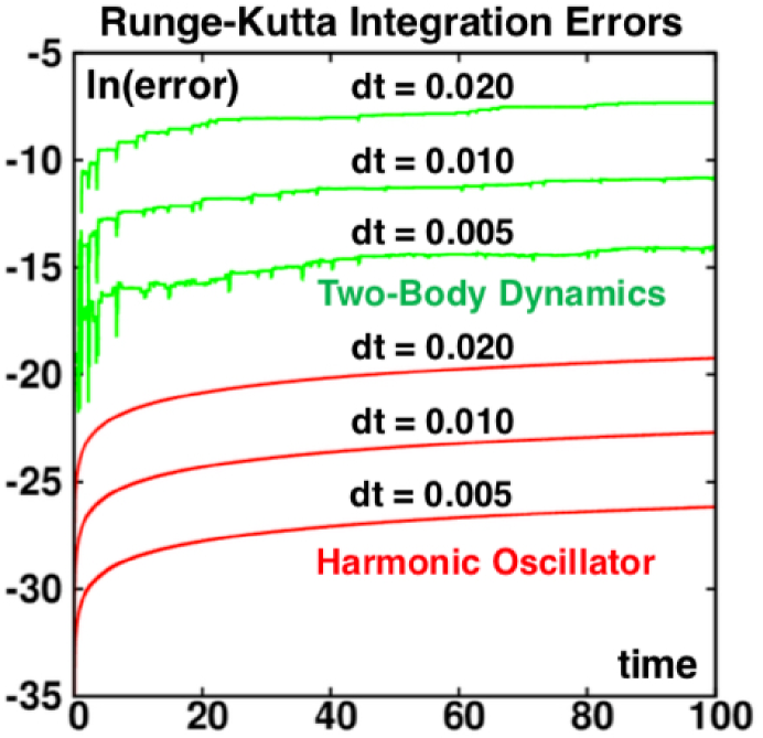
Figure 4: Comparison of the time-dependent error in $q^{2}+p^{2}$ for the harmonic oscillator (below) and the periodic two-body equilibrium problem (above), with an initial energy equal to unity in the latter case. The analytic oscillator solution shows that the energy error at a fixed time varies as $dt^{5}$, which the numerical work for two bodies nicely confirms. Although the two-body error increases less regularly, being dominated by the collisions, it is clear that the same error analysis applies in that case. Replicating these results is a useful debugging exercise for both these equilibrium Hamiltonian problems.

A bit of experimentation shows that a timestep $dt=0.005$ provides good energy conservation. At a time of 1000 the initial energy of unity has decayed to 0.9999937. This time-dependent energy decay is illustrated in Figure 3, at the left for the oscillator and at the right for the two-body problem. The two are also compared on a logarithmic scale in Figure 4 with similar shapes, though the oscillator results are certainly smoother.

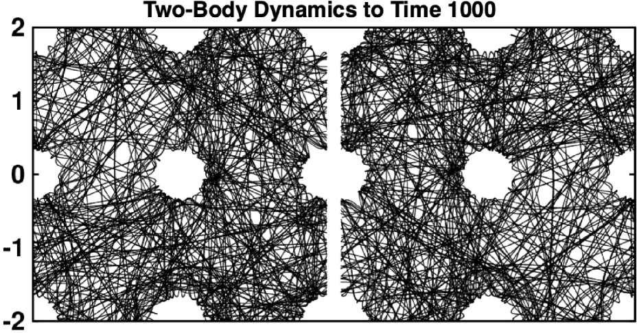
Figure 5: 200,000 points along the equilibrium Hamiltonian $(x,y)$ trajectories for Particle 1 (at the left) and Particle 2 (at the right). Notice the inversion symmetry resulting from the center-of-mass constraints described in the text. The total energy of unity is conserved here. The eight neighboring cells in this case are arranged in a fixed square lattice corresponding to zero strain. Initially the two particles are separated as in Figure 1 with $r=2$, $p_{x}=\mp 0.8$, and $p_{y}=\mp 0.6$, giving $E=1$. The Runge-Kutta timestep is 0.005.

The jumps in the two-body energy, visible in both figures, occur at the collisional turning points. In spite of the relative simplicity of this problem the long-time two-body trajectories illustrated in Figure 5 suggest that there is sufficient chaos in this problem to provide a near-ergodic coordinate distribution. Although the apparent phase-space dimensionality here is eight, much more than the three required for chaos, this equilibrium problem is actually just three-dimensional ! The two-body problem, with the center-of-mass fixed, or equivalently, expressed in relative coordinates, can be reduced to a four-dimensional problem. It could be viewed as the constant-energy motion of a mass-point particle within a periodic $4\times 4$ square with four fixed particles at the corners controlling the mass point’s motion. Conservation of energy further restricts that motion, however expressed, to a three-dimensional energy shell, the actual minimum for chaos. In fact isoenergetic simulations with unit energy show no tendency to approach either of the two collisionless nonchaotic solutions:

$$\{\ x=\pm t\ ;\ y=\pm 1\ ;\ p_{x}=\pm 1\ ;\ p_{y}=0\ \}\ ;\{\ x=\pm 1\ ;\ y=\pm t\ ;\ p_{x}=0\ ;\ p_{y}=\pm 1\ \}\ .$$

In these hypothetical collisionless cases the motion would parallel either of the two coordinate axes, $x$ or $y$.

The chaotic equilibrium problem, just described and pictured in Figure 5 is a useful stepping stone toward the stationary two-body nonequilibrium shear flow that is our goal. Let us consider next the modelling of a steadily moving periodic boundary. Incorporating this driving mechanism will help us simulate a “stationary”, actually time-periodic, nonequilibrium flow. The moving boundary introduces a new variable, the phase or “strain” of the motion, which can be reset to zero when the coordinates in all nine cells regain their perfect square-lattice symmetry.

There is a second barrier to stationarity. Because the moving boundaries do viscous “work” on the two particles in the central cell we will need to “thermostat” the motion to avoid a relatively rapid divergence of the kinetic energy. We will use a Nosé-Hoover thermostat force, $-\zeta p$ to control the kinetic energy. With the addition of a moving boundary and a thermostat our two-body equilibrium model is converted to a nonequilibrium steady flow. We describe its characteristics next. For simplicity we restrict our description to the case of unit strain rate so that the locations of the periodic-image cells repeat at integral values of the time.

IV Nonequilibrium Shear Flow with Two Particles

To reach our goal of “The Simplest Viscous Flow” requires two additions to the equations of motion and corresponding modifications of the integrator. Applying the Runge-Kutta algorithm to shear flow requires augmenting the motion equations to include [1] the explicit time dependence of the boundary conditions and [2] the control of the kinetic energy. Let us consider the modifications in more detail.

IV.1 Imposing a Fixed Strain Rate on the Dynamics

In introducing shear the three square cells with $-2<y<+2$ obey the usual periodic boundary conditions in the $x$ direction. The $y$ direction is different. The shearing motion of three square cells above and three below the central cells is induced by giving the twelve particles in the upper and lower cells additional velocities equal to the product of the strain rate and the cell height: $\dot{x}=p_{x}+4$ above, $\dot{x}=p_{x}-4$ below. We choose to restrict the cell-to-cell strain [ $\epsilon=(\Delta x/\Delta y)$ relative to the perfect square-lattice structure ] of the nine cells of Figure 1 to lie in the range from $-0.5<\epsilon<+0.5$. From the numerical standpoint simply resetting the strain, $+(1/2)\rightarrow-(1/2)$, every 200 steps, prevents the loss of significant figures in the horizontal coordinates $x$. Otherwise simulations with billions of timesteps, corresponding to strains on the order of millions, would erode the accuracy of the horizontal coordinates.

By limiting the strain to lie between the two extreme values $\mp(1/2)$ shown in the figure, it is guaranteed that the nearest-neighbor image of Particle 1 lies uniquely in one of the nine cells shown. Likewise for Particle 2. Thus the nearest-image potential and forces can both be computed for the central-cell Particles 1 and 2 by selecting the minimum-distance particle pair out of the nine possibilities. The unique pair $(x_{ij},y_{ij})$ which minimizes the separation $\sqrt{(x_{ij}^{2}+y_{ij}^{2})}$ is selected from the nine possibilities whenever the righthandsides of the differential equations are calculated, four times within every Runge-Kutta timestep.

IV.2 Imposing a Fixed Time-Averaged Temperature on the Dynamics

We choose a basic time-reversible Nosé-Hoover thermostat to control the temperature. In the time-reversed version both the momenta and the friction coefficient $\zeta$ change signs. For simplicity we choose a thermostat relaxation time of unity in the $\dot{\zeta}$ equation. The thermostatted motion equations are the following, where $T$ is a specified constant target temperature:

$$\{\ \dot{x}=p_{x}+\dot{\epsilon}y\ ;\ \dot{y}=p_{y}\ ;\ \dot{p}_{x}=F_{x}-\zeta p_{x}\ ;\ \dot{p}_{y}=F_{y}-\dot{\epsilon}p_{x}-\zeta p_{y}\ \}\ ;\$$

$$\dot{\zeta}=K-NT\ {\rm where}\ K=\sum(p_{x}^{2}+p_{y}^{2})/2\ .$$

These equations are time-reversible. To see this note first that the overdot “$\ {}^{\bf.}\$” signifies a time derivative so that ($\dot{x},\dot{y}$) change signs with the direction of time while ($\dot{p}_{x},\dot{p}_{y}$) and the forces do not. Evidently $\dot{\epsilon}$ must change sign for reversibility, in agreement with our imagining the shear process from $-0.5$ to $+0.5$ being reversed, from $+0.5$ to $-0.5$. Likewise the sign of the friction coefficient must be reversed just as if it were a momentum. In fact, in Nosé’s original derivation of his thermostat equations the friction coefficient was a momentum. Its conjugate variable $s$ is Nosé’s “time-scaling variable”, which behaved like a coordinate. Though the motion equations just given are patently time-reversible we will see, and come to understand, that the reversibility is illusory, and if attempted will succeed for only a relatively short time.

In this shear flow problem there is a competition between the driving shear force, characterized by the strainrate $\dot{\epsilon}$, and the damping activity of the thermostat, characterized by $\zeta$. These two forces represent work and heat respectively. $\epsilon$ provides work and the thermostat variable $\zeta$ on average extracts the resulting irreversible heating, maintaining a kinetic temperature $2T=\langle\ K\ \rangle=\langle\ (p_{1}^{2}+p_{2}^{2})/2\ \rangle$. With a strainrate of unity a short computation shows that a thermostated kinetic energy of 0.3 provides a longtime chaotic solution.

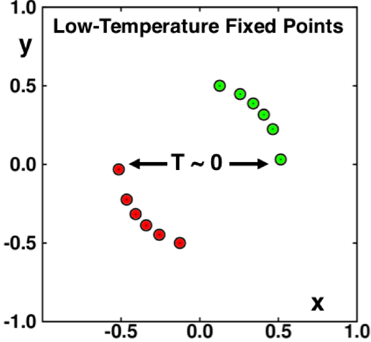
Figure 6: Particle locations for the fixed points at $p^{2}$-based kinetic energies from 0.00 to 0.25 in steps of 0.05 with strainrate unity. At a fixed point the horizontal motion vanishes so that $\dot{x}=p_{x}+y=0$. For Particle 1 the $y$ coordinate is $-\sqrt{K}$, precisely cancelling the horizontal momentum. As the vertical momentum vanishes too $p_{x}^{2}=K=2T$. Convergence at $T=0$ is poor while at kinetic energies from 0.05 to 0.25 convergence to machine accuracy is rapid and accurate. The timestep is 0.005 and the friction coefficient obeys the motion equation $\dot{\zeta}=K-2T$.

At lower temperatures an interesting phenomenon ensues. Low temperature favors an interparticle spacing of unity, the energy minimum. Figure 6 displays exactly this. At lower temperatures, with kinetic energies in the range from 0.25 down to zero, the energy minimum becomes irresistable and the fractal distributions, like those generated at 0.30 and higher, collapse to a fixed point in the nine-dimensional phase space. Such points correspond to an interparticle separation barely exceeding unity, and close to the potential minimum for the interacting Particles 1 and 2. The two particles occupy fixed points on a curve approximating a circle, with diameter slightly greater than unity.

As a consequence, once sufficiently cooled, Particles 1 and 2 no longer can interact with their periodic images to the sides or above or below, for which a central-box separation of the particles greater than 2 is required. Thus low-temperature simulations are no longer representative of boundary-driven shear. Figure 6 shows these unphysical fixed-point solutions. With this thermostat model the “temperature” is entirely taken up by $p_{x}^{2}$ and exactly cancels the coordinate-dependent contribution $\dot{\epsilon}y$ to $\dot{x}$. Meanwhile $p_{y}$ and $\dot{y}$ vanish.

$$\dot{x}=p_{x}+\dot{\epsilon}\times y=0.5+(1.0\times-0.5)=0\ (\rm{For}\ 2T=K=0.25\ {\rm and}\ \dot{\epsilon}=1)\ .$$

Because our pair potential has its maximum value $2^{6}-2^{4}=48$ at $r=0$ it is likewise evident that coupling with the boundary will have a much diminished effect at sufficiently high temperatures. The high-temperature limit is simply uniform over the $4\times 4$ square, assuming sufficient perturbation from the thermostat to favor irrational coordinates and momenta over the rational. Chaotic viscous flow can only exist when both the driving and the dissipative influences on the motion are comparable, so that their time-averaged contributions cancel.

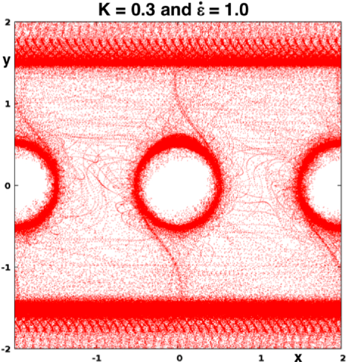
Figure 7: $(x_{1},y_{1})=(-x_{2},-y_{2})$ coordinates at unit shear strain rate with $\langle\ K\ \rangle=0.3$ and $dt=0.005$. The motion shown here covers a simulation from time 50,000 to time 100,000 as represented by one million equally-spaced points.

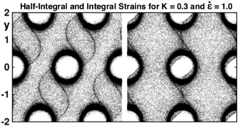
Figure 8: $(x_{1},y_{1})=(-x_{2},-y_{2})$ coordinates at integral (right) and half-integral (left) shear strains from the last half of a 200,000,000 timestep simulation at unit strainrate and averaged kinetic energy 0.3. One million points are shown.

Figure 7 pictures an $(x,y)$ projection of the fractal distribution at $K=2T=0.30$. In the figure the six boundary-cell images of Particles 1 and 2 in the cells above and below the central cell are swept from left to right (above) and right to left (below) accounting for the smearing of probability at the top and bottom of the central cell. Figure 8 shows superpositions of snapshots taken every 200 steps (corresponding to a unit increase in $\epsilon=\dot{\epsilon}t$). Just two of the 200 different phases, at integral and half-integral strains respectively, making up a unit time interval, are shown in the figure. Evidently the probability density is periodic (with period 200 steps here) in time so that a detailed microstate description would need to include the phase of the motion as well as the the values of the coordinates and momenta of Particles 1 and 2.

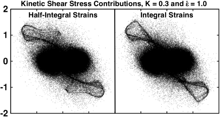
Figure 9: $(p_{x_{1}},p_{y_{1}})=(-p_{x_{2}},-p_{y_{2}})$ momenta at integral (right) and half-integral (left) strains from shear strains beginning at $10^{5}$ and finishing at $10^{6}$. The timestep is 0.005, the averaged kinetic energy $\langle\ K\ \rangle=0.3=2T$, and the shear strain rate $\dot{\epsilon}=(du_{x}/dt)$ is unity. $\dot{\zeta}=K-0.3$. Evidently the velocity distribution is time-periodic and sensitive to the phase of the boundary cells. Here 900,000 points are shown in each panel, selected from the time interval from 100,000 to 1,000,000.

Figure 9 shows two phases of the two-body momentum distribution. The kinetic part of the pressure tensor $P_{xy}$ is proportional to the summed values of $p_{x}p_{y}$, identical for the two particles in our model. The figure shows that the product is, on average, negative, as is required for agreement with continuum mechanics where the shear stress, the negative of $P_{xy}$, is equal to the product of the strain rate and the (positive) coefficient of shear viscosity.

V Describing the Results of The Nonequilibrium Simulations

V.1 Paradoxical Nonequilibrium Phase-Volume Changes

Let us consider the nonequilibrium shearing motion, time-averaged over many repetitions of the boundary time-periodicity in five-dimensional space, $\{x_{1},y_{1},p_{x_{1}},p_{y_{1}},\zeta\}$. Averaging the comoving dilation rate in this phase space for an infinitesimal five-dimensional volume element $\otimes$ gives an empirical inevitable inequality:

$$\langle\ (\dot{\otimes}/\otimes)\ \rangle=\langle\ (\partial\dot{x}_{1}/\partial x_{1})+(\partial\dot{y}_{1}/\partial y_{1})+(\partial\dot{p}_{x_{1}}/\partial p_{x_{1}})+(\partial\dot{p}_{y_{1}}/\partial p_{y_{1}})+(\partial\dot{\zeta}/\partial\zeta)\ \rangle=$$

$$0+0-\langle\ \zeta\ \rangle-\langle\ \zeta\ \rangle+0=-2\langle\ \zeta\ \rangle<0\ .$$

It is characteristic of time-reversible nonequilibrium stationary states that their phase volume inevitably shrinks, as the time-averaged friction coefficient $\zeta$ is invariably positive.

From the computational standpoint a negative friction coefficient would correspond to comoving phase-space growth, numerical instability, and numerical divergence. The inevitable positive friction coefficient, corresponding to comoving shrinkage, and necessary for computational stability, at first looks paradoxical in view of the formal time-reversibility of the motion. To understand, recall that ordinary equilibrium Hamiltonian mechanics conserves the comoving phase volume precisely. This is a consequence of the Hamiltonian motion equations,

$$\{\ \dot{q}=+(\partial{\cal H}/\partial p)\ ;\ \dot{p}=-(\partial{\cal H}/\partial q)\ \}\ \longrightarrow$$

$$\sum[\ (\partial\dot{q}/\partial q)+(\partial\dot{p}/\partial p)\ ]=\sum[\ (\partial/\partial q)(+(\partial{\cal H}/\partial p))+(\partial/\partial p)(-(\partial{\cal H}/\partial q))\ ]\equiv 0\ .$$

At thermal equilibrium, imposed by Nosé-Hoover friction, the time-averaged friction coefficient $\langle\ \zeta\ \rangle$ typically vanishes. Typically the equilibrium $\zeta$ has a Gaussian distribution with zero mean. At equilibrium the logarithm of the phase volume $\otimes$ corresponds to entropy. We will see that this changes away from equilibrium where $\langle\ \zeta\ \rangle$ corresponds to entropy production, and is necessarily positive.

V.2 A Microscopic Version of the Second Law of Thermodynamics

Away from equilibrium, with driving forces and a compensating nonHamiltonian friction coefficient, the comoving dilation rate $(\dot{\otimes}/\otimes)$ is nonzero. The internal energy $\Phi+K$ and the phase volume are no longer constant. To prevent the divergence of both energy and phase volume the mean friction coefficient is necessarily, though paradoxically, positive. This positive friction, in the face of reversibility, is the microscopic version of the Second Law of Thermodynamics, describing the conversion of work to heat. The reversed version of this shearing process would be a violation of that law. This consonance of reversible microscopic dynamics with macroscopic thermodynamics was at first surprising and controversial, but ultimately became both edifying and satisfying, a major result obtained by analyzing the nonequilibrium simulations pioneered by Ashurst. For two early time-reversible one-body “work-to-heat” simulations obeying the Second Law see References 9 and 10.

V.3 The Nature of Nonequilibrium Lyapunov Spectra

From the standpoint of dynamical systems the loss of phase volume is an expected feature for models generating fractal distributions, but only rarely are these models time-reversibleb11 ; b12 . An investigation of the Lyapunov spectrum for fractal distributions invariably results in a negative sum, even in formally time-reversible cases. The negative sum signals a collapse of phase volume to a zero-volume fractal, limit cycle, or fixed point.

A worthy research goal is the Lyapunov analysis of the family of five-dimensional flow equations with ranges of strain rates $\{\ \dot{\epsilon}\ \}$ and temperatures $\{\ T\ \}$:

$$\{\ \dot{x}=p_{x}+\dot{\epsilon}y\ ;\ \dot{y}=p_{y}\ ;\ \dot{p}_{x}=F_{x}-\zeta p_{x}\ ;\ \dot{p}_{y}=F_{y}-\dot{\epsilon}p_{x}-\zeta p_{y}\ \}\ ;\$$

$$\dot{\zeta}=(K/T)-1\ {\rm where}\ K=(p_{x}^{2}+p_{y}^{2})/2\ .$$

The averaged phase-space dilation rate, $\dot{\otimes}$, can be written in terms of the five long-time-averaged Lyapunov exponents,

$$\langle\ (\dot{\otimes}/\otimes)\ \rangle=-2\langle\ \zeta\ \rangle=\langle\ \lambda_{1}+\lambda_{2}+\lambda_{3}+\lambda_{4}+\lambda_{5}\ \rangle\ .$$

Exactly this same equation holds instantaneously though the corresponding “local” values of the exponents depend upon the chosen coordinate system.

The instantaneous values of the five Lyapunov exponents result from the analysis of growth rates for five orthogonal time-dependent vectors in the space, $\{\ \delta_{1}\ \dots\ \delta_{5}\ \}$. Evidently the entire range of phase-space dimensionalities from 0 (a fixed point) to 5 (ergodic coverage, which should result for reasonable combinations of temperature with small strain rates) could be analyzed. We heartily recommend such studies to our readers. These simple dynamical problems are a relatively complex interesting area ripe for study. Surely a periodic symmetric two-body problem is indeed the simplest viscous flow.

V.4 The Relevance of Time-Reversible Maps

In 1996 Hoover, Kum, and Posch constructed and analyzed the results of several time-reversible mapsb13 . Those maps were all defined in a two-dimensional unit square with $-(1/2)<(x,y)<+(1/2)$. Shears, for instance, obeyed the maps ${\bf X(x,y)}$, similar to the shearing considered here, and ${\bf Y(x,y)}$:

$${\bf X(x,y)}:x\rightarrow x^{\prime}=x+\epsilon y\ ;\ y\rightarrow y^{\prime}=y\ ;$$

$${\bf Y(x,y)}:x\rightarrow x^{\prime}=x\ ;\ y\rightarrow y^{\prime}=y+\epsilon x\ .$$

In these two-dimensional cartesian maps $x$ represents a coordinate and $y$ a momentum so that time can be reversed by changing the sign of $y$, analogous to reversing time at a fixed configuration. In this map modelling of time reversibility it is convenient to introduce the time-reversal map ${\bf T}$:

$${\bf T}(x,y):x\rightarrow x^{\prime}=x\ ;\ y\rightarrow y^{\prime}=-y\ .$$

With this definition ${\bf T}$ and its inverse ${\bf T^{-1}}$ are one and the same. In fact any map ${\bf M}(x,y)$ is time-reversible if its inverse is the sequence of operations going backward in time, ${\bf TMT}$, so that ${\bf MM^{-1}}(x,y)={\bf M^{-1}M}(x,y)=(x,y)$.

The 1996 work showed that the mapping ${\bf XYYX}$ was ergodic, with constant density throughout the unit square. Differently, and significantly, the mapping ${\bf XYPYX}$, where ${\bf P}$ was both time-reversible and included regions of density expansion and contraction, produced fractal distributions, ergodic for small deviations from the ${\bf XYYX}$ equilibrium and with an information dimension reduced quadratically in the driving deviation away from equilibrium. Thus the two-dimensional time-reversible maps already contain a mechanism for irreversibility resembling that found in the present “simple” five-dimensional viscous flows.

VI Acknowledgment

We thank Clint Sprott, Karl Travis, and Kris Wojciechowski for their readings of a previous draft. In particular Karl pointed out the importance of two-dimensional maps for the understanding of the irreversibility of the present five-dimensional nonequilibrium flows. A particularly compelling map is the compressible Baker Map, described in two arXiv articles, 1909.04526, “Random Walk Equivalence to the Compressible Baker Map and the Kaplan-Yorke Approximation to Its Information Dimension” and 1910.12642, “2020 Ian Snook Prize Problem : Three Routes to the Information Dimensions for a One-Dimensional Stochastic Random Walk and for an Equivalent Prototypical Two-Dimensional Baker Map”. As no suitable entries for the latter problem were received we again offer a Snook-Prize cash award of one thousand United States dollars for the best work addressing the 2020 problem received during the calendar year 2021. See our “$1000 SNOOK PRIZES FOR 2021: The Information Dimensions of a Two-Dimensional Baker Map”, Computational Methods in Science and Technology 21, 93-94 (2021).

VII Addendum of 8 July 2021

Karl suggested that we include the second-order Runge-Kutta oscillator solution, with

QNEW = Q + P*DT - Q*(DT*DT/2) ; PNEW = P - Q*DT - P*(DT*DT/2) .

The solution is:

$$[q_{n},p_{n}]=[1+(dt^{4}/4)]^{n/2}[+\cos(n\lambda),-\sin(n\lambda)]\ {\rm with}$$

$$\lambda\equiv\arctan\frac{dt}{[1-(dt^{2}/2)]}\ .$$

Because this oscillator amplitude now increases exponentially in time the lack of molecular dynamics simulations using second-order Runge-Kutta algorithms is unsurprising!

References

- (1) T. C. Germann and K. Kadau, “Trillion-Atom Molecular Dynamics Becomes a Reality”, Journal of Modern Physics C 19, 1315-1319 (2008).
- (2) W. T. Ashurst, Dense Fluid Shear Viscosity and Thermal Conductivity via Nonequilibrium Molecular Dynamics (University of California, Davis, 1974) 187 pages.
- (3) S. Nosé, “A Unified Formulation of the Constant Temperature Molecular Dynamics Method”, The Journal of Chemical Physics 81, 511-519 (1984).
- (4) S. Nosé “Molecular Dynamics Method for Simulations in the Canonical Ensemble”, Molecular Physics 52, 255-268 (1984).
- (5) Wm. G. Hoover, “Canonical Dynamics. Equilibrium Phase-Space Distributions”, Physical Review A 31, 1695-1697 (1985).
- (6) W. G. Hoover, “Adiabatic Hamiltonian Deformation, Linear Response Theory, and Nonequilibrium Molecular Dynamics” in Systems Far from Equilibrium, editor L. Garrido, (Springer-Verlag, Berlin, 1980).
- (7) K. P. Travis, W. G. Hoover, C. G. Hoover, and A. B. Hass, “What is Liquid? [in two dimensions]”, Computational Methods in Science and Technology 27, 5-23 (2021).
- (8) Wm. G. Hoover and C. G. Hoover, “Comparison of Very Smooth Cell-Model Trajectories Using Five Symplectic and Two Runge-Kutta Integrators”, Computational Methods in Science and Technology 21, 109-116 (2015).
- (9) B. L. Holian, W. G. Hoover, and H. A. Posch, “Resolution of Loschmidt’s Paradox: The Origin of Irreversible Behavior in Reversible Atomistic Dynamics”, Physical Review Letters 59, 10-13 (1987).
- (10) W. G. Hoover, H. A. Posch, B. L. Holian, M. J. Gillan, M. Mareschal, and C. M. Massobrio, “Dissipative Irreversibility from Nosé’s Reversible Mechanics”, Molecular Simulation 1, 79-86 (I987).
- (11) J. C. Sprott, “Some Simple Chaotic Flows”, Physical Review E 50, R647 (1994).
- (12) W. G. Hoover, ‘Remark on “Some Simple Chaotic Flows” ’, Physical Review E 51, 759-760 (1995).
- (13) W. G. Hoover, O. Kum, and H. A. Posch, “Time-Reversible Dissipative Ergodic Maps”, Physical Review E 53, 2123-2129 (1996).