OptiDICE: Offline Policy Optimization via
Stationary Distribution Correction Estimation

OptiDICE: Offline Policy Optimization via
Stationary Distribution Correction Estimation
(Supplementary Material)

Abstract

We consider the offline reinforcement learning (RL) setting where the agent aims to optimize the policy solely from the data without further environment interactions. In offline RL, the distributional shift becomes the primary source of difficulty, which arises from the deviation of the target policy being optimized from the behavior policy used for data collection. This typically causes overestimation of action values, which poses severe problems for model-free algorithms that use bootstrapping. To mitigate the problem, prior offline RL algorithms often used sophisticated techniques that encourage underestimation of action values, which introduces an additional set of hyperparameters that need to be tuned properly. In this paper, we present an offline RL algorithm that prevents overestimation in a more principled way. Our algorithm, OptiDICE, directly estimates the stationary distribution corrections of the optimal policy and does not rely on policy-gradients, unlike previous offline RL algorithms. Using an extensive set of benchmark datasets for offline RL, we show that OptiDICE performs competitively with the state-of-the-art methods.

1 Introduction

The availability of large-scale datasets has been one of the important factors contributing to the recent success in machine learning for real-world tasks such as computer vision (Deng et al., 2009; Krizhevsky et al., 2012) and natural language processing (Devlin et al., 2019). The standard workflow in developing systems for typical machine learning tasks is to train and validate the model on the dataset, and then to deploy the model with its parameter fixed when we are satisfied with training. This offline training allows us to address various operational requirements of the system without actual deployment, such as acceptable level of prediction accuracy rate once the system goes online.

However, this workflow is not straightforwardly applicable to the standard setting of reinforcement learning (RL) (Sutton & Barto, 1998) because of the online learning assumption: the RL agent needs to continuously explore the environment and learn from its trial-and-error experiences to be properly trained. This aspect has been one of the fundamental bottlenecks for the practical adoption of RL in many real-world domains, where the exploratory behaviors are costly or even dangerous, e.g. autonomous driving (Yu et al., 2020b) and clinical treatment (Yu et al., 2020a).

Offline RL (also referred to as batch RL) (Ernst et al., 2005; Lange et al., 2012; Fujimoto et al., 2019; Levine et al., 2020) casts the RL problem in the offline training setting. One of the most relevant areas of research in this regard is the off-policy RL (Lillicrap et al., 2016; Haarnoja et al., 2018; Fujimoto et al., 2018), since we need to deal with the distributional shift resulting from the trained policy being deviated from the policy used to collect the data. However, without the data continuously collected online, this distributional shift cannot be reliably corrected and poses a significant challenge to RL algorithms that employ bootstrapping together with function approximation: it causes compounding overestimation of the action values for model-free algorithms (Fujimoto et al., 2019; Kumar et al., 2019), which arises from computing the bootstrapped target using the predicted values of out-of-distribution actions. To mitigate the problem, most of the current offline RL algorithms have proposed sophisticated techniques to encourage underestimation of action values, introducing an additional set of hyperparameters that needs to be tuned properly (Fujimoto et al., 2019; Kumar et al., 2019; Jaques et al., 2019; Lee et al., 2020; Kumar et al., 2020).

In this paper, we present an offline RL algorithm that essentially eliminates the need to evaluate out-of-distribution actions, thus avoiding the problematic overestimation of values. Our algorithm, Offline Policy Optimization via Stationary DIstribution Correction Estimation (OptiDICE), estimates stationary distribution ratios that correct the discrepancy between the data distribution and the optimal policy’s stationary distribution. We first show that such optimal stationary distribution corrections can be estimated via minimax optimization that does not involve sampling from the target policy. Then, we derive and exploit the closed-form solution to the sub-problem of the aforementioned minimax optimization, which reduces the overall problem into an unconstrained convex optimization, and thus greatly stabilizing our method. To the best of our knowledge, OptiDICE is the first deep offline RL algorithm that optimizes policy purely in the space of stationary distributions, rather than in the space of either Q-functions or policies (Nachum et al., 2019b). In the experiments, we demonstrate that OptiDICE performs competitively with the state-of-the-art methods using the D4RL offline RL benchmarks (Fu et al., 2021).

2 Background

We consider the reinforcement learning problem with the environment modeled as a Markov Decision Process (MDP) $M=\langle S,A,T,R,p_{0},\gamma\rangle$ (Sutton & Barto, 1998), where $S$ is the set of states $s$, $A$ is the set of actions $a$, $R:S\times A\rightarrow\mathbb{R}$ is the reward function, $T:S\times A\rightarrow\Delta(S)$ is a transition probability, $p_{0}\in\Delta(S)$ is an initial state distribution, and $\gamma\in[0,1]$ is a discount factor. The policy $\pi:S\rightarrow\Delta(A)$ is a mapping from state to distribution over actions. While $T(s,a)$ and $\pi(s)$ indicate distributions by definition, we let $T(s^{\prime}|s,a)$ and $\pi(a|s)$ denote their evaluations for brevity. For the given policy $\pi$, the stationary distribution $d^{\pi}$ is defined as

$$d^{\pi}(s,a)=\begin{cases}(1-\gamma)\sum\limits_{t=0}^{\infty}\gamma^{t}\Pr(s_{t}=s,a_{t}=a)&\text{if }\gamma<1,\\ \lim\limits_{T\rightarrow\infty}\frac{1}{T+1}\sum\limits_{t=0}^{T}\Pr(s_{t}=s,a_{t}=a)&\text{if }\gamma=1,\end{cases}$$

where $s_{0}\sim p_{0}$ and $a_{t}\sim\pi(s_{t}),s_{t+1}\sim T(s_{t},a_{t})$ for all time step $t$. The goal of RL is to learn an optimal policy that maximizes rewards through interactions with the environment: $\max_{\pi}\mathbb{E}_{(s,a)\sim d^{\pi}}[R(s,a)]$. The value functions of policy $\pi$ is defined as $Q^{\pi}(s,a):=\mathbb{E}_{\pi,M}\left[\sum_{t=0}^{\infty}\gamma^{t}R(s_{t},a_{t})|s_{0}=s,a_{0}=a\right]$ and $V^{\pi}(s):=\mathbb{E}_{a\sim\pi(s)}[Q^{\pi}(s,a)]$, where the action-value function $Q^{\pi}$ is a unique solution of the Bellman equation:

$$Q^{\pi}(s,a)=R(s,a)+\gamma\mathbb{E}_{\begin{subarray}{c}s^{\prime}\sim T(s,a)\\ a^{\prime}\sim\pi(s^{\prime})\end{subarray}}[Q^{\pi}(s^{\prime},a^{\prime})].$$

In offline RL, the agent optimizes the policy from static dataset $D=\{(s_{i},a_{i},r_{i},s_{i}^{\prime})\}_{i=1}^{N}$ collected before the training phase. We denote the empirical distribution of the dataset by $d^{D}$ and will abuse the notation $d^{D}$ to represent $s\sim d^{D}$, $(s,a)\sim d^{D}$, and $(s,a,s^{\prime})\sim d^{D}$.

Prior offline model-free RL algorithms, exemplified by (Fujimoto et al., 2019; Kumar et al., 2019; Wu et al., 2019; Lee et al., 2020; Kumar et al., 2020; Nachum et al., 2019b), rely on estimating Q-values for optimizing the target policy. This procedure often yields unreasonably high Q-values due to the compounding error from bootstrapped estimation with out-of-distribution actions sampled from the target policy (Kumar et al., 2019).

3 OptiDICE

In this section, we present Offline Policy Optimization via Stationary DIstribution Correction Estimation (OptiDICE). Instead of the optimism in the face of uncertainty principle (Szita & Lörincz, 2008) in online RL, we discourage the uncertainty as in most offline RL algorithms (Kidambi et al., 2020; Yu et al., 2020c); otherwise, the resulting policy may fail to improve on the data-collection policy, or even suffer from severe performance degradation (Petrik et al., 2016; Laroche et al., 2019). Specifically, we consider the regularized policy optimization framework (Nachum et al., 2019b)

$$\pi^{*}:=\operatorname*{arg\,max}_{\pi}\mathbb{E}_{(s,a)\sim d^{\pi}}[R(s,a)]-\alpha D_{f}(d^{\pi}||d^{D}),$$ (1)

where $D_{f}(d^{\pi}||d^{D}):=\mathbb{E}_{(s,a)\sim d^{D}}\left[f\big{(}\frac{d^{\pi}(s,a)}{d^{D}(s,a)}\big{)}\right]$ is the $f$-divergence between the stationary distribution $d^{\pi}$ and the dataset distribution $d^{D}$, and $\alpha>0$ is a hyperparameter that balances between pursuing the reward-maximization and penalizing the deviation from the distribution of the offline dataset (i.e. penalizing distributional shift). We assume $d^{D}>0$ and $f$ being strictly convex and continuously differentiable. Note that we impose regularization in the space of stationary distributions rather than in the space of policies (Wu et al., 2019). However, optimizing for $\pi$ in (1) involves the evaluation of $d^{\pi}$, which is not directly accessible in the offline RL setting.

To make the optimization tractable, we reformulate (1) in terms of optimizing a stationary distribution $d:{S\times A}\rightarrow\mathbb{R}$. For brevity, we consider discounted MDPs ($\gamma<1$) and then generalize the result to undiscounted MDPs ($\gamma=1$). Using $d$, we rewrite (1) as

$$\max_{d}~{} \mathbb{E}_{(s,a)\sim d}[R(s,a)]-\alpha D_{f}(d||d^{D})$$ (2)

$$\mathrm{s.t.}~{} (\mathcal{B}_{*}d)(s)=(1-\gamma)p_{0}(s)+\gamma(\mathcal{T}_{*}d)(s)~{}~{}\forall s,$$ (3)

$$d(s,a)\geq 0~{}~{}\forall s,a,$$ (4)

where $(\mathcal{B}_{*}d)(s):=\sum_{\bar{a}}d(s,\bar{a})$ is a marginalization operator, and $(\mathcal{T}_{*}d)(s):=\sum_{\bar{s},\bar{a}}T(s|\bar{s},\bar{a})d(\bar{s},\bar{a})$ is a transposed Bellman operator. Note that when $\alpha=0$, the optimization (2-4) is exactly the dual formulation of the linear program (LP) for finding an optimal policy of the MDP (Puterman, 1994), where the constraints (3-4) are often called the Bellman flow constraints. Once the optimal stationary distribution $d^{*}$ is obtained, we can recover the optimal policy $\pi^{*}$ in (1) from $d^{*}$ by $\pi^{*}(a|s)=\frac{d^{*}(s,a)}{\sum_{\bar{a}}d^{*}(s,\bar{a})}$.

We then obtain the following Lagrangian for the constrained optimization problem in (2-4):

$$\max_{d\geq 0}\min_{\nu}\mathbb{E}_{(s,a)\sim d}[R(s,a)]-\alpha D_{f}(d||d^{D})$$ (5)

$$~{}~{}~{}~{}~{}~{}+\textstyle\sum\limits_{s}\nu(s)\Big{(}(1-\gamma)p_{0}(s)+\gamma(\mathcal{T}_{*}d)(s)-(\mathcal{B}_{*}d)(s)\Big{)},$$

where $\nu(s)$ are the Lagrange multipliers. Lastly, we eliminate the direct dependence on $d$ and $\mathcal{T}_{*}$ by rearranging the terms in (5) and optimizing the distribution ratio $w$ instead of $d$:

$$\mathbb{E}_{(s,a)\sim d}[R(s,a)]-\alpha D_{f}(d||d^{D})$$

$$+\textstyle\sum\limits_{s}\nu(s)\Big{(}(1-\gamma)p_{0}(s)+\gamma(\mathcal{T}_{*}d)(s)-(\mathcal{B}_{*}d)(s)\Big{)}$$

$$= \textstyle(1-\gamma)\mathbb{E}_{s\sim p_{0}}[\nu(s)]+\mathbb{E}_{(s,a)\sim d^{D}}\left[-\alpha f\left(\frac{d(s,a)}{d^{D}(s,a)}\right)\right]$$ (6)

$$+\textstyle\sum\limits_{s,a}d(s,a)\Big{(}\underbrace{R(s,a)+\gamma(\mathcal{T}\nu)(s,a)-(\mathcal{B}\nu)(s,a)}_{\small\begin{subarray}{c}=:e_{\nu}(s,a)\text{~{}~{}(`advantage' using $\nu$)}\end{subarray}}\Big{)}$$

$$= \textstyle(1-\gamma)\mathbb{E}_{s\sim p_{0}}[\nu(s)]+\mathbb{E}_{(s,a)\sim d^{D}}\left[-\alpha f\left(\frac{d(s,a)}{d^{D}(s,a)}\right)\right]$$

$$\textstyle+\mathbb{E}_{(s,a)\sim d^{D}}\Big{[}\underbrace{\tfrac{d(s,a)}{d^{D}(s,a)}}_{\small\begin{subarray}{c}=:w(s,a)\end{subarray}}\big{(}e_{\nu}(s,a)\big{)}\Big{]}$$

$$= (1-\gamma)\mathbb{E}_{s\sim p_{0}}[\nu(s)]+\mathbb{E}_{(s,a)\sim d^{D}}\left[-\alpha f\big{(}w(s,a)\big{)}\right]$$

$$+\mathbb{E}_{(s,a)\sim d^{D}}\left[w(s,a)\big{(}e_{\nu}(s,a)\big{)}\right]=:L(w,\nu).$$ (7)

The first equality holds due to the property of the adjoint (transpose) operators $\mathcal{B}_{*}$ and $\mathcal{T}_{*}$, i.e. for any $\nu$,

$$\textstyle\sum\limits_{s}\nu(s)(\mathcal{B}_{*}d)(s) =\textstyle\sum\limits_{s,a}d(s,a)(\mathcal{B}\nu)(s,a),$$

$$\textstyle\sum\limits_{s}\nu(s)(\mathcal{T}_{*}d)(s) =\textstyle\sum\limits_{s,a}d(s,a)(\mathcal{T}\nu)(s,a),$$

where $(\mathcal{T}\nu)(s,a)=\sum_{s^{\prime}}T(s^{\prime}|s,a)\nu(s^{\prime})$ and $(\mathcal{B}\nu)(s,a)=\nu(s)$. Note that $L(w,\nu)$ in (7) does not involve expectation over $d$, but only expectation over $p_{0}$ and $d^{D}$, which allows us to perform optimization only with the offline data.

Remark.

The terms in (7) will be estimated only by using the samples from the dataset distribution $d^{D}$:

$$\hat{L}(w,\nu):=(1-\gamma)\mathbb{E}_{s\sim p_{0}}[\nu(s)]$$ (8)

$$+\mathbb{E}_{(s,a,s^{\prime})\sim d^{D}}\left[-\alpha f\big{(}w(s,a)\big{)}+w(s,a)\big{(}\hat{e}_{\nu}(s,a,s^{\prime})\big{)}\right].$$

Here, $\hat{e}_{\nu}(s,a,s^{\prime}):=R(s,a)+\gamma\nu(s^{\prime})-\nu(s)$ is a single-sample estimation of advantage $e_{\nu}(s,a)$. On the other hand, prior offline RL algorithms often involve estimations using out-of-distribution actions sampled from the target policy, e.g. employing a critic to compute bootstrapped targets for the value function. Thus, our method is free from the compounding error in the bootstrapped estimation due to using out-of-distribution actions.

In short, OptiDICE solves the problem

$$\max_{w\geq 0}\min_{\nu}L(w,\nu),$$ (9)

where the optimal solution $w^{*}$ of the optimization (9) represents the stationary distribution corrections between the optimal policy’s stationary distribution and the dataset distribution: $w^{*}(s,a)=\frac{d^{\pi^{*}}(s,a)}{d^{D}(s,a)}$.

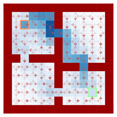
(a) Stationary Dist. $d^{\pi_{\!{}_{D}}}$

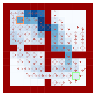
(b) Empirical Dist. $d^{D}$

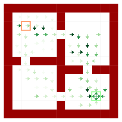
(c) OptiDICE $w^{*}$

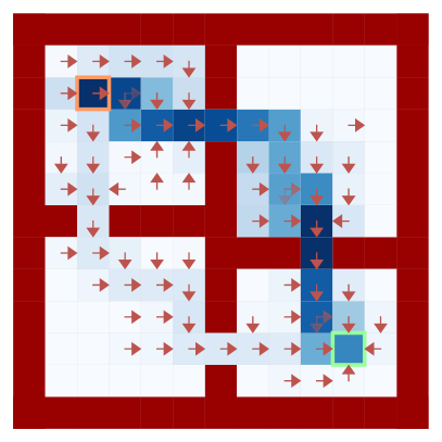
(d) Estimated $\hat{d}^{\pi^{*}}$

Figure 1: Illustrative example of how OptiDICE estimates the optimal policy’s stationary distribution in the Four Rooms domain (Sutton et al., 1999; Nachum et al., 2019b). The initial state and the goal state are denoted by orange and green squares, respectively. Based on a sub-optimal data-collection policy $\pi_{\!{}_{D}}$, which induces $d^{\pi_{\!{}_{D}}}$ shown in (a), a static dataset is sampled and its empirical distribution $d^{D}$ ($\neq d^{\pi_{\!{}_{D}}}$) shown in (b). The opacity of each square is determined by the state marginals of each stationary distribution, where the opacity of the arrow shows the policy induced by each stationary distribution. By multiplying the OptiDICE $w^{*}$ obtained by solving (9) (shown in (c)), a near-optimal policy $\pi^{*}$ is obtained from $\hat{d}^{\pi^{*}}(s,a)=d^{D}(s,a)w^{*}(s,a)$ shown in (d).

3.1 A closed-form solution

When the state and/or action spaces are large or continuous, it is a standard practice to use function approximators to represent terms such as $w$ and $\nu$, and perform gradient-based optimization of $L$. However, this could break nice properties for optimizing $L$, such as concavity in $w$ and convexity in $\nu$, which causes numerical instability and poor convergence for the maximin optimization (Goodfellow et al., 2014). We mitigate this issue by obtaining the closed-form solution of the inner optimization, which reduces the overall problem into a unconstrained convex optimization.

Since the optimization problem (2-4) is an instance of convex optimization, one can easily show that the strong duality holds by the Slater’s condition (Boyd et al., 2004). Hence we can reorder the optimization from maximin to minimax:

$$\min_{\nu}\max_{w\geq 0}L(w,\nu).$$ (10)

Then, for any $\nu$, a closed-form solution to the inner maximization of (10) can be derived as follows:

Proposition 1.

The closed-form solution of the inner maximization of (10), $w_{\nu}^{*}:=\operatorname*{arg\,max}_{w\geq 0}L(w,\nu)$, is

$$w_{\nu}^{*}(s,a)=\max\left(0,(f^{\prime})^{-1}\left(\frac{e_{\nu}(s,a)}{\alpha}\right)\right)~{}~{}\forall s,a,$$ (11)

where $(f^{\prime})^{-1}$ is the inverse function of the derivative $f^{\prime}$ of $f$ and is strictly increasing by strict convexity of $f$. (Proof in Appendix A.)

A closer look at (11) reveals that that for a fixed $\nu$, the optimal stationary distribution correction $w_{\nu}^{*}(s,a)$ is larger for a state-action pair with larger advantage $e_{\nu}(s,a)$. This solution property has a natural interpretation as follows. As $\alpha\rightarrow 0$, the term in (6) becomes the Lagrangian of the primal LP for solving the MDP, where $d(s,a)$ serve as Lagrange multipliers to impose constraints $R(s,a)+\gamma(\mathcal{T}\nu)(s,a)\leq\nu(s)~{}\forall s,a$. Also, each $\nu(s)$ serves as the optimization variable representing the optimal state value function (Puterman, 1994). Thus, $e_{\nu^{*}}(s,a)=Q^{*}(s,a)-V^{*}(s)$, i.e. the advan-tage function of the optimal policy, should be zero for the optimal action while it should be lower for sub-optimal actions. For $\alpha>0$, the convex regularizer $f\big{(}\frac{d(s,a)}{d^{D}(s,a)}\big{)}$ in (6) relaxes those constraints into soft ones, but it still prefers the actions with higher $e_{\nu^{*}}(s,a)$ over those with lower $e_{\nu^{*}}(s,a)$. From this perspective, $\alpha$ adjusts the softness of the constraints $e_{\nu}(s,a)\leq 0~{}\forall s,a$, and $f$ determines the relation between advantages and stationary distribution corrections.

Finally, we reduce the nested optimization in (10) to the following single minimization problem by plugging $w_{\nu}^{*}$ into $L(w,\nu)$:

$$\min_{\nu}L(w_{\nu}^{*},\nu)=(1-\gamma)\mathbb{E}_{s\sim p_{0}}[\nu(s)]$$ (12)

$$~{}~{}~{}+\mathbb{E}_{(s,a)\sim d^{D}}\left[-\alpha f\Big{(}\max\Big{(}0,(f^{\prime})^{-1}\big{(}\tfrac{1}{\alpha}e_{\nu}(s,a)\big{)}\Big{)}\Big{)}\right]$$

$$~{}~{}~{}+\mathbb{E}_{(s,a)\sim d^{D}}\left[\max\Big{(}0,(f^{\prime})^{-1}\big{(}\tfrac{1}{\alpha}e_{\nu}(s,a)\big{)}\Big{)}\big{(}e_{\nu}(s,a)\big{)}\right].$$

Proposition 2.

$L(w_{\nu}^{*},\nu)$ is convex with respect to $\nu$. (Proof in Appendix B.)

The minimization of this convex objective can be performed much more reliably than the nested minimax optimization problem. For practical purposes, we use the following objective that can be easily optimized via sampling from $D$:

$$\tilde{L}(\nu):=(1-\gamma)\mathbb{E}_{s\sim p_{0}}[\nu(s)]$$ (13)

$$+\mathbb{E}_{(s,a,s^{\prime})\sim d^{D}}\bigg{[}-\alpha f\Big{(}\max\Big{(}0,(f^{\prime})^{-1}\big{(}\tfrac{1}{\alpha}\hat{e}_{\nu}(s,a,s^{\prime})\big{)}\Big{)}\Big{)}$$

$$+\max\Big{(}0,(f^{\prime})^{-1}\big{(}\tfrac{1}{\alpha}\hat{e}_{\nu}(s,a,s^{\prime})\big{)}\Big{)}\big{(}\hat{e}_{\nu}(s,a,s^{\prime})\big{)}\bigg{]}.$$

However, careful readers may notice that $\tilde{L}(\nu)$ can be a biased estimate of our target objective $L(w_{\nu}^{*},\nu)$ in (12) due to non-linearity of $(f^{\prime})^{-1}$ and double-sample problem (Baird, 1995) in $L(w_{\nu}^{*},\nu)$. We justify $\tilde{L}(\nu)$ by formally showing that $\tilde{L}(\nu)$ is the upper bound of $L(w_{\nu}^{*},\nu)$:

Corollary 3.

$\tilde{L}(\nu)$ in (13) is an upper bound of $L(w_{\nu}^{*},\nu)$ in (12), i.e. $L(w_{\nu}^{*},\nu)\leq\tilde{L}(\nu)$ always holds, where equality holds when the MDP is deterministic. (Proof in Appendix B.)

Illustrative example

Figure 1 outlines how our approach works in the Four Rooms domain (Sutton et al., 1999) where the agent aims to navigate to a goal location in a maze composed of four rooms. We collected static dataset $D$ consisting of $50$ episodes with maximum time step $50$ using the data-collection policy $\pi_{\!{}_{D}}=0.5\pi_{\mathrm{true}}^{*}+0.5\pi_{\mathrm{rand}}$, where $\pi_{\mathrm{true}}^{*}$ is the optimal policy of the underlying true MDP and $\pi_{\mathrm{rand}}$ is the random policy sampled from the Dirichlet distribution, i.e. $\pi_{\mathrm{rand}}(s)\sim\mathrm{Dir}(1,1,1,1)~{}\forall s$.

In this example, we explicitly constructed Maximum Likelihood Estimate (MLE) MDP $\hat{M}$ based on the static dataset $D$. We then obtained $\nu^{*}$ by minimizing  (12) where $\hat{M}$ was used to exactly compute $e_{\nu}(s,a)$. Then, $w_{\nu^{*}}^{*}$ was estimated directly via Eq. (11) (Figure 1(c)). Finally, $w^{*}$ was multiplied by $d^{D}$ to correct $d^{D}$ towards an optimal policy, resulting in $\hat{d}^{\pi^{*}}$, which is the stationary distribution of the estimated optimal policy (Figure 1(d)). For tabular MDPs, the global optima $(\nu^{*},w^{*})$ can always be obtained. We describe these experiments on OptiDICE for finite MDPs in Appendix C.

3.2 Stationary distribution correction estimation with function approximation

Based on the results from the previous section, we assume that $\nu$ and $w$ are parameterized by $\theta$ and $\phi$, respectively, and that both models are sufficiently expressive, e.g. using deep neural networks. Using these models, we optimize $\theta$ by

$$\min_{\theta}J_{\nu}(\theta):=\min_{\theta}\tilde{L}(\nu_{\theta}).$$ (14)

After obtaining the optimizing solution $\theta^{*}$, we need a way to evaluate $w^{*}(s,a)=\frac{d^{\pi^{*}}(s,a)}{d^{D}(s,a)}$ for any $(s,a)$ to finally obtain the optimal policy $\pi^{*}$. However, the closed-form solution $w_{\nu_{\theta}}^{*}(s,a)$ in Proposition 1 can be evaluated only on $(s,a)$ in $D$ since it requires both $R(s,a)$ and $\mathbb{E}_{s^{\prime}\sim T(s,a)}[\nu_{\theta}(s^{\prime})]$ to evaluate the advantage $e_{\nu}$. Therefore, we use a parametric model $e_{\phi}$ that approximates the advantage inside the analytic formula presented in (11), so that

$$w_{\phi}(s,a):=\max\left(0,(f^{\prime})^{-1}\left(\frac{e_{\phi}(s,a)}{\alpha}\right)\right).$$ (15)

We consider two options to optimize $\phi$ once we obtain $\nu_{\theta}$ from Eq. (14). First, $\phi$ can be optimized via

$$\min_{\phi}J_{w}(\phi;\theta):=\min_{\phi}-\hat{L}(w_{\phi},\nu_{\theta})$$ (16)

which corresponds to solving the original minimax problem (10). We also consider

$$\min_{\phi} ~{}J_{w}^{\mathrm{MSE}}(\phi;\theta)$$

$$:=\min_{\phi}\mathbb{E}_{\begin{subarray}{c}(s,a,s^{\prime})\sim d^{D}\end{subarray}}\Big{[}\big{(}e_{\phi}(s,a)-\hat{e}_{\nu_{\theta}}(s,a,s^{\prime})\big{)}^{2}\Big{]},$$ (17)

which minimizes the mean squared error (MSE) between the advantage $e_{\phi}(s,a)$ and the target induced by $\nu_{\theta}$. We observe that using either $J_{w}$ or $J_{w}^{\mathrm{MSE}}$ works effectively, which will be detailed in our experiments. In our implementation, we perform joint training of $\theta$ and $\phi$, rather than optimizing $\phi$ after convergence of $\theta$.

3.3 Policy extraction

As the last step, we need to extract the optimal policy $\pi^{*}$ from the optimal stationary distribution corrections $w_{\phi}(s,a)=\frac{d^{\pi^{*}}(s,a)}{d^{D}(s,a)}$. While the optimal policy can be easily obtained by $\pi^{*}(a|s)=\frac{d^{D}(s,a)w_{\phi}(s,a)}{\sum_{\bar{a}}d^{D}(s,\bar{a})w_{\phi}(s,\bar{a})}$ for tabular domains, this procedure is not straightforwardly applicable to continuous domains.

One of the ways to address continuous domains is to use importance-weighted behavioral cloning: we optimize the parameterized policy $\pi_{\psi}$ by maximizing the log-likelihood on $(s,a)$ that would be sampled from the optimal policy $\pi^{*}$:

$$\max_{\psi} ~{}\mathbb{E}_{(s,a)\sim d^{\pi^{*}}}[\log\pi_{\psi}(a|s)]$$

$$~{}~{}~{}~{}~{}~{}~{}=\max_{\psi}\mathbb{E}_{(s,a)\sim d^{D}}\left[\textstyle w_{\phi}(s,a)\log\pi_{\psi}(a|s)\right].$$

Despite its simplicity, this approach does not work well in practice, since $\pi_{\psi}$ will be trained only on samples from the intersection of the supports of $d^{\pi^{*}}$ and $d^{D}$, which becomes very scarce when $\pi^{*}$ deviates significantly from the data collection policy $\pi_{\!{}_{D}}$.

We thus use the information projection (I-projection) for training the policy:

$$\min_{\psi}~{}\mathbb{KL}\left(d^{D}(s)\pi_{\psi}(a|s)||d^{D}(s)\pi^{*}(a|s)\right),$$ (18)

where we replace $d^{\pi^{*}}(s)$ by $d^{D}(s)$ for $d^{\pi^{*}}(s,a)$. This results in minimizing the discrepancy between $\pi_{\psi}(a|s)$ and $\pi^{*}(a|s)$ on the stationary distribution over states from $\pi_{\!{}_{D}}$. This approach is motivated by the desideratum that the policy $\pi_{\psi}$ should be trained at least on the states observed in $D$ to be robust upon deployment. Now, rearranging the terms in (18), we obtain

$$\mathbb{KL}\left(d^{D}(s)\pi_{\psi}(a|s)||d^{D}(s)\pi^{*}(a|s)\right)$$

$$=-\mathbb{E}_{\begin{subarray}{c}s\sim d^{D}\\ a\sim\pi_{\psi}(s)\end{subarray}}\bigg{[}\log\underbrace{\frac{d^{*}(s,a)}{d^{D}(s,a)}}_{=w_{\phi}(s,a)}-\log\frac{\pi_{\psi}(a|s)}{\pi_{\!{}_{D}}(a|s)}-\underbrace{\log\frac{d^{*}(s)}{d^{D}(s)}}_{\text{constant for $\pi$}}\bigg{]}$$

$$=-\mathbb{E}_{\begin{subarray}{c}s\sim d^{D}\\ a\sim\pi_{\psi}(s)\end{subarray}}\left[\log w_{\phi}(s,a)-\mathbb{KL}(\pi_{\psi}(\bar{a}|s)||\pi_{\!{}_{D}}(\bar{a}|s))\right]+C$$

$$=:J_{\pi}(\psi;\phi,\pi_{\!{}_{D}})$$ (19)

We can interpret this I-projection objective as a KL-regularized actor-critic architecture (Fox et al., 2016; Schulman et al., 2017), where $\log w_{\phi}(s,a)$ taking the role of the critic and $\pi_{\psi}$ being the actor. Note that I-projection requires us to evaluate $\pi_{\!{}_{D}}$ for the KL regularization term. For this, we employ another parameterized policy $\pi_{\beta}$ to approximate $\pi_{\!{}_{D}}$, trained via simple behavioral cloning (BC).

3.4 Generalization to $\gamma=1$

For $\gamma=1$, our original problem (2-4) for the stationary distribution $d$ is an ill-posed problem: for any $d$ that satisfies the Bellman flow constraints (3-4) and a constant $c\geq 0$, $cd$ also satisfies the Bellman flow constraints (3-4) (Zhang et al., 2020a). We address this issue by adding additional normalization constraint $\sum_{s,a}d(s,a)=1$ to (2-4). By using analogous derivation from (2) to (10) with the normalization constraint—introducing a Lagrange multiplier $\lambda\in\mathbb{R}$ and changing the variable $d$ to $w$—we obtain the following minimax objective for $w$, $\nu$ and $\lambda$:

$$\min_{\nu,\lambda}\max_{w\geq 0}L(w,\nu,\lambda)$$

$$\hskip 10.0pt:=L(w,\nu)+\lambda(1-\mathbb{E}_{(s,a)\sim d^{D}}[w(s,a)])$$

$$\hskip 10.0pt=(1-\gamma)\mathbb{E}_{s\sim p_{0}}[\nu(s)]+\mathbb{E}_{(s,a)\sim d^{D}}[-\alpha f(w(s,a))]$$

$$\hskip 10.0pt~{}~{}~{}~{}~{}-\mathbb{E}_{(s,a)\sim d^{D}}[w(s,a)(e_{\nu}(s,a)-\lambda))]+\lambda.$$ (20)

Similar to (8), we define $\hat{L}(w,\nu,\lambda)$, an unbiased estimator for $L(w,\nu,\lambda)$ such that

$$\hat{L}(w,\nu,\lambda):=(1-\gamma)\mathbb{E}_{s\sim p_{0}}[\nu(s)]+\lambda$$ (21)

$$+\mathbb{E}_{(s,a,s^{\prime})\sim d^{D}}\left[-\alpha f\big{(}w(s,a)\big{)}+w(s,a)\big{(}\hat{e}_{\nu,\lambda}(s,a,s^{\prime})\big{)}\right],$$

where $\hat{e}_{\nu,\lambda}(s,a,s^{\prime}):=\hat{e}_{\nu}(s,a,s^{\prime})-\lambda$. We then derive a closed-form solution for the inner maximization in (20):

Proposition 4.

The maximizer $w_{\nu,\lambda}^{*}:{S\times A}\rightarrow\mathbb{R}$ of the inner optimization of (20), which is defined by $w_{\nu,\lambda}^{*}:=\operatorname*{arg\,max}_{w\geq 0}L(w,\nu,\lambda)$, is

$$w_{\nu,\lambda}^{*}(s,a)=\max\left(0,(f^{\prime})^{-1}\left(\frac{e_{\nu}(s,a)-\lambda}{\alpha}\right)\right).$$

(Proof in Appendix D.)

Similar to (13), we minimize the biased estimate $\tilde{L}(\nu,\lambda)$, which is an upper bound of $L(w_{\nu,\lambda}^{*},\nu,\lambda)$, by applying the closed-form solution from Proposition 4:

$$\tilde{L}(\nu,\lambda):=(1-\gamma)\mathbb{E}_{s\sim p_{0}}[\nu(s)]$$ (22)

$$+\mathbb{E}_{(s,a,s^{\prime})\sim d^{D}}\bigg{[}-\alpha f\Big{(}\max\big{(}0,(f^{\prime})^{-1}\big{(}\tfrac{1}{\alpha}\hat{e}_{\nu,\lambda}(s,a,s^{\prime})\big{)}\big{)}\Big{)}$$

$$+\max\Big{(}0,(f^{\prime})^{-1}\big{(}\tfrac{1}{\alpha}\hat{e}_{\nu,\lambda}(s,a,s^{\prime})\big{)}\Big{)}\big{(}\hat{e}_{\nu,\lambda}(s,a,s^{\prime})\big{)}\bigg{]}+\lambda.$$

By using the above estimators, we correspondingly update our previous objectives for $\theta$ and $\phi$ as follows. First, the objective for $\theta$ is modified to

$$\min_{\theta}J_{\nu}(\theta,\lambda):=\min_{\theta}\tilde{L}(\nu_{\theta},\lambda).$$ (23)

For $\phi$, we modify our approximator in (15) by including the Lagrangian $\lambda^{\prime}\in\mathbb{R}$:

$$w_{\phi,\lambda^{\prime}}(s,a):=\max\left(0,(f^{\prime})^{-1}\left(\frac{e_{\phi}(s,a)-\lambda^{\prime}}{\alpha}\right)\right).$$

Note that $\lambda^{\prime}\neq\lambda$ is used to stabilize the learning process. For optimizing over $\phi$, the minimax objective (16) is modified as

$$\min_{\phi}J_{w}(\phi,\lambda^{\prime};\theta):=\min_{\phi}-\hat{L}(w_{\phi,\lambda^{\prime}},\nu_{\theta},\lambda^{\prime}),$$ (24)

while the same objective $J_{w}^{\mathrm{MSE}}(\phi;\theta)$ in (17) is used for the MSE objective. We additionally introduce learning objectives for $\lambda$ and $\lambda^{\prime}$, which is required for the normalization constraint discussed in this subsection:

$$\min_{\lambda}J_{\nu}(\theta,\lambda)~{}~{}~{}\text{ and }~{}~{}~{}\min_{\lambda^{\prime}}J_{w}(\phi,\lambda^{\prime};\theta).$$ (25)

Finally, by using the above objectives in addition to BC objective and policy extraction objective in (19), we describe our algorithm, OptiDICE, in Algorithm 1, where we train neural network parameters via stochastic gradient descent. In our algorithm, we use a warm-up iteration—optimizing all networks except $\pi_{\psi}$—to prevent $\pi_{\psi}$ from its converging to sub-optimal policies during its initial training. In addition, we empirically observed that using the normalization constraint stabilizes OptiDICE’s learning process even for $\gamma<1$, thus we used the normalization constraint in all experiments (Zhang et al., 2020a).

Algorithm 1 OptiDICE

0:  A dataset $D:=\{(s_{i},a_{i},r_{i},s_{i}^{\prime})\}_{i=1}^{N}$, a set of initial states $D_{0}:=\{s_{0,i}\}_{i=1}^{N_{0}}$, neural networks $\nu_{\theta}$ and $e_{\phi}$ with parameters $\theta$ and $\phi$, learnable parameters $\lambda$ and $\lambda^{\prime}$, policy networks $\pi_{\beta}$ and $\pi_{\psi}$ with parameter $\beta$ and $\psi$, a learning rate $\eta$

1:  for each iteration do

2:     Sample mini-batches from $D$ and $D_{0}$, respectively.

3:     Compute $\theta$-gradient to optimize (23):

$$g_{\theta}\approx\nabla_{\theta}J_{\nu}(\theta,\lambda)$$

4:     Compute $\phi$-gradient for either one of objectives:

$$g_{\phi} \approx\nabla_{\phi}J_{w}(\phi,\lambda^{\prime};\theta)$$ (minimax obj. (24))

$$g_{\phi} \approx\nabla_{\phi}J_{w}^{\mathrm{MSE}}(\phi;\theta)$$ (MSE obj. (17))

5:     Compute $\lambda$ and $\lambda^{\prime}$ gradients to optimize (25):

$$g_{\lambda}\approx\nabla_{\lambda}J_{\nu}(\theta,\lambda),g_{\lambda^{\prime}}\approx\nabla_{\lambda^{\prime}}J_{w}(\phi,\lambda^{\prime};\theta)$$

6:     Compute $\beta$-gradient $g_{\beta}$ for BC.

7:     Compute $\psi$-gradient via (19) (policy extraction):

$$g_{\psi}\approx\nabla_{\psi}J_{\pi}(\psi;\phi,\pi_{\beta})$$

8:     Perform SGD updates:   $\displaystyle\theta$ $\displaystyle\leftarrow\theta-\eta g_{\theta},$ $\displaystyle\phi$ $\displaystyle\leftarrow\phi-\eta g_{\phi},$   $\displaystyle\lambda$ $\displaystyle\leftarrow\lambda-\eta g_{\lambda},$ $\displaystyle\lambda^{\prime}$ $\displaystyle\leftarrow\lambda^{\prime}-\eta g_{\lambda^{\prime}},$   $\displaystyle\beta$ $\displaystyle\leftarrow\beta-\eta g_{\beta},$ $\displaystyle\psi$ $\displaystyle\leftarrow\psi-\eta g_{\psi}.$

9:  end for

9:  $\nu_{\theta}\approx\nu^{*}$, $w_{\phi,\lambda^{\prime}}\approx w^{*}$, $\pi_{\psi}\approx\pi^{*}$,

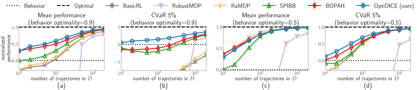
Figure 2: Performance of tabular OptiDICE and baseline algorithms in random MDPs. For baselines, we use BasicRL (a model-based RL computing an optimal policy via MLE MDP), Robust MDP (Nilim & El Ghaoui, 2005; Iyengar, 2005), Reward-adjusted MDP (RaMDP) (Petrik et al., 2016), SPIBB (Laroche et al., 2019), BOPAH (Lee et al., 2020). For varying numbers of trajectories and two types of data-collection policies ($\zeta=0.9,0.5$), the mean and the 5%-CVaR of normalized performances for 10,000 runs are reported with 95% confidence intervals. OptiDICE performs better than (for $\zeta=0.9$) or on par with (for $\zeta=0.5$) the baselines in the mean performance measure, while always outperforming the baselines in the CVaR performance measure.

4 Experiments

In this section, we evaluate OptiDICE for both tabular and continuous MDPs. For the $f$-divergence, we chose $f(x)=\frac{1}{2}(x-1)^{2}$, i.e. $\chi^{2}$-divergence for the tabular-MDP experiment, while we use its softened version for continuous MDPs (See Appendix E for details).

4.1 Random MDPs (tabular MDPs)

We validate tabular OptiDICE’s efficiency and robustness using randomly generated MDPs by following the experimental protocol from Laroche et al. (2019) and Lee et al. (2020) (See Appendix F.1.). We consider a data-collection policy $\pi_{\!{}_{D}}$ characterized by the behavior optimality parameter $\zeta$ that relates to $\pi_{\!{}_{D}}$’s performance $\zeta V^{*}(s_{0})+(1-\zeta)V^{\pi_{\mathrm{unif}}}(s_{0})$ where $\pi_{\mathrm{unif}}$ denotes the uniformly random policy. We evaluate each algorithm in terms of the normalized performance of the policy $\pi$, given by $(V^{*}(s_{0})-V^{\pi_{\!{}_{D}}}(s_{0}))/(V^{\pi}(s_{0})-V^{\pi_{\!{}_{D}}}(s_{0}))$, which intuitively measures the performance enhancement of $\pi$ over $\pi_{\!{}_{D}}$. Each algorithm is tested for 10,000 runs, and their mean and 5% conditional value at risk (5%-CVaR) are reported, where the mean of the worst 500 runs is considered for 5%-CVaR. Note that CVaR implicitly stands for the robustness of each algorithm.

We describe the performance of tabular OptiDICE and baselines in Figure 2. For $\zeta=0.9$, where $\pi_{\!{}_{D}}$ is near-deterministic and thus $d^{D}$’s support is relatively small, OptiDICE outperforms the baselines in both mean and CVaR (Figure 2(a),(b)). For $\zeta=0.5$, where $\pi_{\!{}_{D}}$ is highly stochastic and thus $d^{D}$’s support is relatively large, OptiDICE outperforms the baselines in CVaR, while performing competitively in mean. In summary, OptiDICE was more sample-efficient and stable than the baselines.

Table 1: Normalized performance of OptiDICE compared with the best model-free baseline in the D4RL benchmark tasks (Fu et al., 2021). In the Best baseline column, the algorithm with the best performance among 8 algorithms (offline SAC (Haarnoja et al., 2018), BEAR (Kumar et al., 2019), BRAC (Wu et al., 2019), AWR (Peng et al., 2019), cREM (Agarwal et al., 2020), BCQ (Fujimoto et al., 2019), AlgaeDICE (Nachum et al., 2019b), CQL (Kumar et al., 2020)) is presented, taken from (Fu et al., 2021). OptiDICE achieved highest scores in 7 tasks.

D4RL Task	Best baseline		OptiDICE
maze2d-umaze	88.2	Offline SAC	111.0
maze2d-medium	33.8	BRAC-v	145.2
maze2d-large	40.6	BRAC-v	155.7
hopper-random	12.2	BRAC-v	11.2
hopper-medium	58.0	CQL	94.1
hopper-medium-replay	48.6	CQL	36.4
hopper-medium-expert	110.9	BCQ	111.5
walker2d-random	7.3	BEAR	9.9
walker2d-medium	81.1	BRAC-v	21.8
walker2d-medium-replay	26.7	CQL	21.6
walker2d-medium-expert	111.0	CQL	74.8
halfcheetah-random	35.4	CQL	11.6
halfcheetah-medium	46.3	BRAC-v	38.2
halfcheetah-medium-replay	47.7	BRAC-v	39.8
halfcheetah-medium-expert	64.7	BCQ	91.1

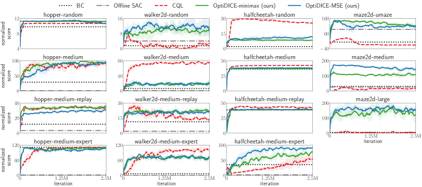
Figure 3: Performance of BC, offline SAC (Haarnoja et al., 2018), CQL (Kumar et al., 2020), OptiDICE-minimax (= OptiDICE with minimax objective in (16)) and OptiDICE-MSE (= OptiDICE with MSE objective in (17)) on D4RL benchmark (Fu et al., 2021) for $\gamma=0.99$. For BC and offline SAC, we use the result reported in D4RL paper (Fu et al., 2021). For CQL and OptiDICE, we provide learning curves for each algorithm where the policy is optimized during 2,500,000 iterations. For CQL, we use the original code by authors with hyperparameters reported in the CQL paper (Kumar et al., 2020). OptiDICE strictly outperforms CQL on 6 tasks, while performing on par with CQL on 4 tasks. We report mean scores and their 95% confidence intervals obtained from 5 runs for each task.

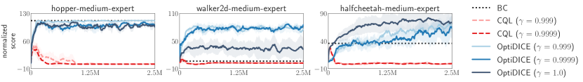
Figure 4: Performance of BC, CQL and OptiDICE (with MSE objective in (17)) in D4RL benchmark (Fu et al., 2021) for $\gamma=0.999,0.9999$ and $1.0$, where the hyperparameters other than $\gamma$ are the same as those in Figure 3.

4.2 D4RL benchmark (continuous control tasks)

We evaluate OptiDICE in continuous MDPs using D4RL offline RL benchmarks (Fu et al., 2021). We use Maze2D (3 tasks) and Gym-MuJoCo (12 tasks) domains from the D4RL dataset (See Appendix F.2 for task description). We interpret terminal states as absorbing states and use the absorbing-state implementation proposed by Kostrikov et al. (2019a). For obtaining $\pi_{\beta}$ discussed in Section 3.3, we use the tanh-squashed mixture of Gaussians policy $\pi_{\beta}$ to embrace the multi-modality of data collected from heterogeneous policies. For the target policy $\pi_{\psi}$, we use a tanh-squashed Gaussian policy, following conservative Q Learning (CQL) (Kumar et al., 2020)—the state-of-the-art model-free offline RL algorithm. We provide detailed information of the experimental setup in Appendix F.2.

The normalized performance of OptiDICE and the best model-free algorithm for each domain is presented in Table 1, and learning curves for CQL and OptiDICE are shown in Figure 3, where $\gamma=0.99$ used for all algorithms. Most notably, OptiDICE achieves state-of-the-art performance for all tasks in the Maze2D domain, by a large margin. In Gym-MuJoCo domain, OptiDICE achieves the best mean performance for 4 tasks (hopper-medium, hopper-medium-expert, walker2d-random, and halfcheetah-medium-expert). Another noteworthy observation is that OptiDICE overwhelmingly outperforms AlgaeDICE (Nachum et al., 2019b) in all domains (Table 1 and Table 3 in Appendix for detailed performance of AlgaeDICE), although both AlgaeDICE and OptiDICE stem from the same objective in (1). This is because AlgaeDICE optimizes a nested max-min-max problem, which can suffer from severe overestimation by using out-of-distribution actions and numerical instability. In contrast, OptiDICE solves a simpler minimization problem and does not rely on out-of-distribution actions, exhibiting stable optimization.

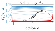
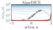
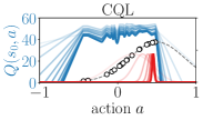
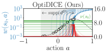
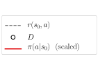
Figure 5: Illustration on overestimation. $r(s_{0},a)$ is a ground-truth reward, $D$ is a sampled offline dataset, and $\pi(a|s_{0})$ is the policy density normalized by its maximum.

$$\textstyle\textbf{AlgaeDICE}~{}~{}\big{(}e_{\nu}^{{\color[rgb]{1,0,0}\pi}}(s,a):=r(s,a)+\gamma\mathbb{E}_{\begin{subarray}{c}s^{\prime}\sim T(s,a),{\color[rgb]{1,0,0}a^{\prime}\sim\pi(s^{\prime})}\end{subarray}}[\nu(s^{\prime},{\color[rgb]{1,0,0}a^{\prime}})]-\nu(s,a),~{}~{}\hat{e}_{\nu}(s,a,s^{\prime},a^{\prime}):=r(s,a)+\gamma\nu(s^{\prime},a^{\prime})-\nu(s,a)\big{)}$$

$$\textstyle\hskip 12.0pt{\color[rgb]{1,0,0}\max_{\pi}\min_{\nu}\max_{w}}\mathbb{E}_{\begin{subarray}{c}(s,a)\sim d^{D}\end{subarray}}\big{[}e_{\nu}^{\pi}(s,a)w(s,a)-\alpha f\big{(}w(s,a)\big{)}\big{]}+(1-\gamma)\mathbb{E}_{\begin{subarray}{c}s_{0}\sim p_{0},a_{0}\sim\pi(s_{0})\end{subarray}}\left[\nu(s_{0},a_{0})\right]$$ (26)

$$\textstyle={\color[rgb]{1,0,0}\max_{\pi}\min_{\nu}}\alpha\mathbb{E}_{\begin{subarray}{c}(s,a)\sim d^{D}\end{subarray}}\big{[}f_{*}\big{(}\tfrac{1}{\alpha}e_{\nu}^{\pi}(s,a)\big{)}\big{]}+(1-\gamma)\mathbb{E}_{\begin{subarray}{c}s_{0}\sim p_{0},a_{0}\sim\pi(s_{0})\end{subarray}}\left[\nu(s_{0},a_{0})\right]$$ (27)

$$\textstyle\approx{\color[rgb]{1,0,0}\max_{\pi}\min_{\nu}}\alpha\mathbb{E}_{\begin{subarray}{c}(s,a,s^{\prime})\sim d^{D},a^{\prime}\sim\pi(s^{\prime})\end{subarray}}\big{[}f_{*}\big{(}\tfrac{1}{\alpha}\hat{e}_{\nu}(s,a,s^{\prime},a^{\prime})\big{)}\big{]}+(1-\gamma)\mathbb{E}_{\begin{subarray}{c}s_{0}\sim p_{0},a_{0}\sim\pi(s_{0})\end{subarray}}\left[\nu(s_{0},a_{0})\right]$$ (28)

$$\textstyle\textbf{OptiDICE}~{}~{}\big{(}e_{\nu}(s,a):=r(s,a)+\gamma\mathbb{E}_{s^{\prime}\sim T(s,a)}[\nu(s^{\prime})]-\nu(s),~{}~{}\hat{e}_{\nu}(s,a,s^{\prime}):=r(s,a)+\gamma\nu(s^{\prime})-\nu(s),x_{+}:=\max(0,x)\big{)}$$

$$\textstyle\hskip 12.0pt{\color[rgb]{0,0,1}\min_{\nu}\max_{w\geq 0}}\mathbb{E}_{(s,a)\sim d^{D}}\big{[}e_{\nu}(s,a){\color[rgb]{0,0,0}w(s,a)}-\alpha f\big{(}{\color[rgb]{0,0,0}w(s,a)}\big{)}\big{]}+(1-\gamma)\mathbb{E}_{s_{0}\sim p_{0}}[\nu(s_{0})]$$ (29)

$$\textstyle={\color[rgb]{0,0,1}\min_{\nu}}\mathbb{E}_{(s,a)\sim d^{D}}\big{[}e_{\nu}(s,a){\color[rgb]{0,0,0}(f^{\prime})^{-1}\big{(}\tfrac{1}{\alpha}e_{\nu}(s,a)\big{)}_{+}}-\alpha f\big{(}{\color[rgb]{0,0,0}(f^{\prime})^{-1}\big{(}\tfrac{1}{\alpha}e_{\nu}(s,a)\big{)}_{+}}\big{)}\big{]}+(1-\gamma)\mathbb{E}_{s_{0}\sim p_{0}}[\nu(s_{0})]$$ (30)

$$\textstyle\approx{\color[rgb]{0,0,1}\min_{\nu}}\mathbb{E}_{(s,a,s^{\prime})\sim d^{D}}\big{[}\hat{e}_{\nu}(s,a,s^{\prime}){\color[rgb]{0,0,0}(f^{\prime})^{-1}\big{(}\tfrac{1}{\alpha}\hat{e}_{\nu}(s,a,s^{\prime})\big{)}_{+}}-\alpha f\big{(}{\color[rgb]{0,0,0}(f^{\prime})^{-1}(\tfrac{1}{\alpha}\hat{e}_{\nu}(s,a,s^{\prime}))_{+}}\big{)}\big{]}+(1-\gamma)\mathbb{E}_{s_{0}\sim p_{0}}[\nu(s_{0})]$$ (31)

As discussed in Section 3.4, OptiDICE can naturally be generalized to undiscounted problems ($\gamma=1$). In Figure 4, we vary $\gamma\in\{0.999,0.9999,1.0\}$ to validate OptiDICE’s robustness in $\gamma$ by comparing with CQL in {hopper-medium-expert, walker2d-medium-expert, halfcheetah-medium-expert} (See Appendix G for the results for other tasks). The performance of OptiDICE stays stable, while CQL easily becomes unstable as $\gamma$ increases, due to the divergence of Q-function. This is because OptiDICE uses normalized stationary distribution corrections, whereas CQL learns the action-value function whose values becomes unbounded as $\gamma$ gets close to 1, resulting in numerical instability.

5 Discussion

Current DICE algorithms except for AlgaeDICE (Nachum et al., 2019b) only deal with either policy evaluation (Nachum et al., 2019a; Zhang et al., 2020a, b, b; Yang et al., 2020; Dai et al., 2020) or imitation learning (Kostrikov et al., 2019b), not policy optimization.

Although both AlgaeDICE (Nachum et al., 2019b) and OptiDICE aim to solve $f$-divergence regularized RL, each algorithm solves the problem in a different way. AlgaeDICE relies on off-policy evaluation (OPE) of the intermediate policy $\pi$ via DICE (inner $\min_{\nu}\max_{w}$ of Eq. (26)), and then optimizes $\pi$ via policy-gradient upon the OPE result (outer $\max_{\pi}$ of Eq. (26)), yielding an overall $\max_{\pi}\min_{\nu}\max_{w}$ problem of Eq. (26). Although the actual AlgaeDICE implementation employs an additional approximation for practical optimization, i.e. using Eq. (28) that removes the innermost $\max_{w}$ via convex conjugate and uses a biased estimation of $f_{*}(\mathbb{E}_{s^{\prime},a^{\prime}}[\cdot])$ via $\mathbb{E}_{s^{\prime},a^{\prime}}[f_{*}(\cdot)]$, it still involves nested $\max_{\pi}\min_{\nu}$ optimization, susceptible to instability. In contrast, OptiDICE directly estimates the stationary distribution corrections of the optimal policy, resulting in $\min_{\nu}\max_{w}$ problem of Eq. (29). In addition, our implementation performs the single minimization of Eq. (31) (the biased estimate of $\min_{\nu}$ of (30)), which greatly improves the stability of overall optimization.

To see this, we conduct single-state MDP experiments, where $S=\{s_{0}\}$ is the state space, $A=[-1,1]$ is the action space, $T(s_{0}|s_{0},a)=1$ is the transition dynamics, $r(s_{0},a)$ is a reward function, $\gamma=0.9$, and $D$ is the offline dataset. The blue lines in the figures present the estimates learned by each algorithm (i.e. $Q$, $\nu$, $w$) (Darker colors mean later iterations). Similarly, the red lines visualize the action densities from intermediate policies. In this example, a vanilla off-policy actor-critic (AC) method suffers from the divergence of Q-values due to its TD target being outside the data distribution $d^{D}$. This makes the policy learn toward unreasonably high Q-values outside $d^{D}$. AlgaeDICE with Eq. (28) is no better for small $\alpha$. CQL addresses this issue by lowering the Q-values outside $d^{D}$. Finally, OptiDICE computes optimal stationary distribution corrections $w(s,a)=\tfrac{d^{\pi^{*}}(s,a)}{d^{D}(s,a)}$ by Eq. (31) and Eq. (29) ($\max_{w}(\cdot)$ for $\nu^{*}$). Then, the policy $\pi(a|s)\propto w(s,a)d^{D}(s,a)$ is extracted, automatically ensuring actions to be selected within the support of $d^{D}$ ($\mathrm{supp}(d^{D})$).

Also, note that Eq. (31) of OptiDICE is unbiased (i.e., (31) = (30)) if $T$ is deterministic (Corollary 3). In contrast, Eq. (28) of AlgaeDICE is always biased (i.e., (27) $\neq$ (28)) even for the deterministic $T$, due to its dependence on expectation w.r.t. $\pi$. Our biased objective of Eq. (31) removes the need for double sampling in Eq. (30).

6 Conclusion

We presented OptiDICE, an offline RL algorithm that aims to estimate stationary distribution corrections between the optimal policy’s stationary distribution and the dataset distribution. We formulated the estimation problem as a minimax optimization that does not involve sampling from the target policy, which essentially circumvents the overestimation issue incurred by bootstrapped target with out-of-distribution actions, practiced by most model-free offline RL algorithms. Then, deriving the closed-form solution of the inner optimization, we simplified the nested minimax optimization for obtaining the optimal policy to a convex minimization problem. In the experiments, we demonstrated that OptiDICE performs competitively with the state-of-the-art offline RL baselines.

Appendix A Proof of Proposition 1

We first show that our original problem (2-4) is an instance of convex programming due to the convexity of $f$.

Lemma 5.

The constraint optimization (2-4) is a convex optimization.

Proof.

$$\max_{d}~{} \mathbb{E}_{(s,a)\sim d}[R(s,a)]-\alpha D_{f}(d||d^{D})$$ (2)

$$\mathrm{s.t.}~{} (\mathcal{B}_{*}d)(s)=(1-\gamma)p_{0}(s)+\gamma(\mathcal{T}_{*}d)(s)~{}~{}\forall s,$$ (3)

$$d(s,a)\geq 0~{}~{}\forall s,a,$$ (4)

The objective function $\mathbb{E}_{(s,a)\sim d}[R(s,a)]-\alpha D_{f}(d||d^{D})$ is concave for $d:S\times A\rightarrow\mathbb{R}$ (not only for probability distribution $d\in\Delta(S\times A)$) since $D_{f}(d||d^{D})$ is convex in $d$: for $t\in[0,1]$ and any $d_{1}:{S\times A}\rightarrow\mathbb{R},d_{2}:{S\times A}\rightarrow\mathbb{R}$,

$$D_{f}((1-t)d_{1}+td_{2}||d^{D}) =\sum_{s,a}d^{D}(s,a)f\left((1-t)\frac{d_{1}(s,a)}{d^{D}(s,a)}+t\frac{d_{2}(s,a)}{d^{D}(s,a)}\right)$$

$$<\sum_{s,a}d^{D}(s,a)\left\{(1-t)f\left(\frac{d_{1}(s,a)}{d^{D}(s,a)}\right)+tf\left(\frac{d_{2}(s,a)}{d^{D}(s,a)}\right)\right\}$$

$$=(1-t)D_{f}(d_{1}||d^{D})+tD_{f}(d_{2}||d^{D}),$$

where the strict inequality follows from assuming $f$ is strictly convex. In addition, the equality constraints (3) are affine in $d$, and the inequality constraints (4) are linear and thus convex in $d$. Therefore, our problem is an instance of a convex programming, as we mentioned in Section 3.1. ∎

In addition, by using the strong duality and the change-of-variable from $d$ to $w$, we can rearrange the original maximin optimization to the minimax optimization.

Lemma 6.

We assume that all states $s\in S$ are reachable for a given MDP. Then,

$$\max_{w\geq 0}\min_{\nu}L(w,\nu)=\min_{\nu}\max_{w\geq 0}L(w,\nu).$$

Proof.

Let us define the Lagrangian of the constraint optimization (2-4)

$$\mathcal{L}(d,\nu,\mu):=\mathbb{E}_{(s,a)\sim d}[R(s,a)]-\alpha D_{f}(d||d^{D}) +\sum_{s}\nu(s)\left((1-\gamma)p_{0}(s)+\gamma\sum_{\bar{s},\bar{a}}T(s|\bar{s},\bar{a})d(\bar{s},\bar{a})-\sum_{\bar{a}}d(s,\bar{a})\right)$$

$$+\sum_{s,a}\mu(s,a)d(s,a)$$

with Lagrange multipliers $\nu(s)~{}\forall s$ and $\mu(s,a)~{}\forall s,a$. With the Lagrangian $\mathcal{L}(d,\nu,\mu)$, the original problem (2-4) can be represented by

$$\max_{d\geq 0}\min_{\nu}\mathcal{L}(d,\nu,0)=\max_{d}\min_{\nu,\mu\geq 0}\mathcal{L}(d,\nu,\mu).$$

For an MDP where every $s\in S$ is reachable, there always exists $d$ such that $d(s,a)>0~{}\forall s,a$. From Slater’s condition for convex problems (the condition that there exists a strictly feasible $d$ (Boyd et al., 2004)), the strong duality holds, i.e., we can change the order of optimizations:

$$\max_{d}\min_{\nu,\mu\geq 0}\mathcal{L}(d,\nu,\mu)=\min_{\nu,\mu\geq 0}\max_{d}\mathcal{L}(d,\nu,\mu)=\min_{\nu}\max_{d\geq 0}\mathcal{L}(d,\nu,0).$$

Here, the last equality holds since $\max_{d\geq 0}\mathcal{L}(d,\nu,0)=\max_{d}\min_{\mu\geq 0}\mathcal{L}(d,\nu,\mu)=\min_{\mu\geq 0}\max_{d}\mathcal{L}(d,\nu,\mu)$ for fixed $\nu$ due to the strong duality. Finally, by applying the change of variable $w=d/d^{D}$, we have

$$\max_{w\geq 0}\min_{\nu}L(w,\nu)=\min_{\nu}\max_{w\geq 0}L(w,\nu).$$

∎

Finally, the solution of the inner maximization $\max_{w\geq 0}L(w,\nu)$ can be derived as follows:

Proposition 1.

The closed-form solution of the inner maximization of (10), i.e.

$$w_{\nu}^{*}:=\operatorname*{arg\,max}_{w\geq 0}(1-\gamma)\mathbb{E}_{s\sim p_{0}}[\nu(s)]+\mathbb{E}_{(s,a)\sim d^{D}}\left[-\alpha f\big{(}w(s,a)\big{)}\right]+\mathbb{E}_{(s,a)\sim d^{D}}\left[w(s,a)\big{(}e_{\nu}(s,a)\big{)}\right]$$

is given as

$$w_{\nu}^{*}(s,a)=\max\left(0,(f^{\prime})^{-1}\left(\frac{e_{\nu}(s,a)}{\alpha}\right)\right)~{}~{}\forall s,a,$$ (32)

where $(f^{\prime})^{-1}$ is the inverse function of the derivative $f^{\prime}$ of $f$ and is strictly increasing by strict convexity of $f$.

Proof.

For a fixed $\nu$, let the maximization $\max_{w\geq 0}L(w,\nu)$ be the primal problem. Then, its corresponding dual problem is

$$\max_{w}\min_{\mu\geq 0}L(w,\nu)+\sum_{s,a}\mu(s,a)w(s,a).$$

Since the strong duality holds, satisfying KKT condition is both necessary and sufficient conditions for the solutions $w^{*}$ and $\mu^{*}$ of primal and dual problems (we will use $w^{*}$ and $\mu^{*}$ instead of $w_{\nu}^{*}$ and $\mu_{\nu}^{*}$ for notational brevity).

Condition 1 (Primal feasibility). $w^{*}\geq 0~{}\forall s,a$.

Condition 2 (Dual feasibility). $\mu^{*}\geq 0~{}\forall s,a$.

Condition 3 (Stationarity). $d^{D}(s,a)(-\alpha f^{\prime}(w^{*}(s,a))+e_{\nu}(s,a)+\mu^{*}(s,a))=0~{}\forall s,a$.

Condition 4 (Complementary slackness). $w^{*}(s,a)\mu^{*}(s,a)=0~{}\forall s,a.$

From Stationarity and $d^{D}>0$, we have

$$f^{\prime}(w^{*}(s,a))=\frac{e_{\nu}(s,a)+\mu^{*}(s,a)}{\alpha}~{}\forall s,a$$

and since $f^{\prime}$ is invertible due to the strict convexity of $f$,

$$w^{*}(s,a)=(f^{\prime})^{-1}\left(\frac{e_{\nu}(s,a)+\mu^{*}(s,a)}{\alpha}\right)~{}\forall s,a.$$

Now for fixed $(s,a)\in S\times A$, let us consider two cases: either $w^{*}(s,a)>0$ or $w^{*}(s,a)=0$, where Primal feasibility is always satisfied in either way:

Case 1 ($w^{*}(s,a)>0$). $\mu^{*}(s,a)=0$ due to Complementary slackness, and thus,

$$w^{*}(s,a)=(f^{\prime})^{-1}\left(\frac{e_{\nu}(s,a)}{\alpha}\right)>0.$$

Note that Dual feasibility holds. Since $f^{\prime}$ is a strictly increasing function, $e_{\nu}(s,a)>\alpha f^{\prime}(0)$ should be satisfied if $f^{\prime}(0)$ is well-defined.

Case 2 ($w^{*}(s,a)=0$). $\mu^{*}(s,a)=\alpha f^{\prime}(0)-e_{\nu}(s,a)\geq 0$ due to Stationarity and Dual feasibility, and thus, $e_{\nu}(s,a)\leq\alpha f^{\prime}(0)$ should be satisfied if $f^{\prime}(0)$ is well-defined.

In summary, we have

$$w_{\nu}^{*}(s,a) =\max\left(0,(f^{\prime})^{-1}\left(\frac{e_{\nu}(s,a)}{\alpha}\right)\right).$$

∎

Appendix B Proofs of Proposition 2 and Corollary 3

Proposition 2.

$L(w_{\nu}^{*},\nu)$ is convex with respect to $\nu$.

Proof by Lagrangian duality.

Let us consider Lagrange dual function

$$g(\nu,\mu):=\max_{d}\mathcal{L}(d,\nu,\mu),$$

which is always convex in Lagrange multipliers $\nu,\mu$ since $\mathcal{L}(d,\nu,\mu)$ is affine in $\nu,\mu$. Also, for any $\mu_{1},\mu_{2}\geq 0$ and its convex combination $(1-t)\mu_{1}+t\mu_{2}$ for $0\leq t\leq 1$, we have

$$\min_{\mu\geq 0}g((1-t)\nu_{1}+t\nu_{2},\mu)\leq g((1-t)\nu_{1}+t\nu_{2},(1-t)\mu_{1}+t\mu_{2})\leq(1-t)g(\nu_{1},\mu_{1})+tg(\nu_{2},\mu_{2})$$

by using the convexity of $g(\nu,\mu)$. Since the above statement holds for any $\mu_{1},\mu_{2}\geq 0$, we have

$$\min_{\mu\geq 0}g((1-t)\nu_{1}+t\nu_{2},\mu)\leq(1-t)\min_{\mu_{1}\geq 0}g(\nu_{1},\mu_{1})+t\min_{\mu_{2}\geq 0}g(\nu_{2},\mu_{2}).$$

Therefore, a function

$$G(\nu):=\min_{\mu\geq 0}g(\nu,\mu)=\min_{\mu\geq 0}\max_{d}\mathcal{L}(d,\nu,\mu)=\max_{d\geq 0}\mathcal{L}(d,\nu,0)$$

is convex in $\nu$. By following the change-of-variable, we have

$$\max_{d\geq 0}\mathcal{L}(d,\nu,0)=\max_{w\geq 0}L(w,\nu)=L(\operatorname*{arg\,max}_{w\geq 0}L(w,\nu),\nu)=L(w_{\nu}^{*},\nu)$$

is convex in $\nu$.

∎

Proof by exploiting second-order derivative.

Suppose $((f^{\prime})^{-1})^{\prime}$ is well-defined, where $f$ we consider in this work satisfies the condition. Let us define

$$h(x):=-f\Big{(}\max\Big{(}0,(f^{\prime})^{-1}(x)\Big{)}\Big{)}+\max\Big{(}0,(f^{\prime})^{-1}(x)\Big{)}\cdot x.$$ (33)

Then, $L(w_{\nu}^{*},\nu)$ can be represented by using $h$:

$$L(w_{\nu}^{*},\nu)$$

$$=(1-\gamma)\mathbb{E}_{s\sim p_{0}}[\nu(s)]+\mathbb{E}_{(s,a)\sim d^{D}}\Big{[}-\alpha f\Big{(}\max\Big{(}0,(f^{\prime})^{-1}\big{(}\tfrac{1}{\alpha}e_{\nu}(s,a)\big{)}\Big{)}\Big{)}+\max\Big{(}0,(f^{\prime})^{-1}\big{(}\tfrac{1}{\alpha}e_{\nu}(s,a)\big{)}\Big{)}e_{\nu}(s,a)\Big{]}$$

$$=(1-\gamma)\mathbb{E}_{s\sim p_{0}}[\nu(s)]+\mathbb{E}_{(s,a)\sim d^{D}}\Big{[}\alpha h\Big{(}\tfrac{1}{\alpha}e_{\nu}(s,a)\Big{)}\Big{]}$$ (34)

We prove that $h(x)$ is convex in $x$ by showing $h^{\prime\prime}(x)\geq 0~{}\forall x$. Recall that $f^{\prime}$ is a strictly increasing function by the strict convexity of $f$, which implies that $(f^{\prime})^{-1}$ is also a strictly increasing function.

Case 1. If $(f^{\prime})^{-1}(x)>0~{}\forall x$,

$$h(x) =-f((f^{\prime})^{-1}(x))+(f^{\prime})^{-1}(x)\cdot x,$$

$$h^{\prime}(x) =-\underbrace{f^{\prime}((f^{\prime})^{-1}(x))}_{\text{(identity function)}}((f^{\prime})^{-1})^{\prime}(x)+((f^{\prime})^{-1})^{\prime}(x)\cdot x+(f^{\prime})^{-1}(x)$$

$$=-x\cdot((f^{\prime})^{-1})^{\prime}(x)+((f^{\prime})^{-1})^{\prime}(x)\cdot x+(f^{\prime})^{-1}(x)$$

$$=(f^{\prime})^{-1}(x),$$

$$h^{\prime\prime}(x) =((f^{\prime})^{-1})^{\prime}(x)>0,$$

where $((f^{\prime})^{-1})^{\prime}(x)>0$ since it is the derivative of the strictly increasing function $(f^{\prime})^{-1}$.

Case 2. If $(f^{\prime})^{-1}(x)\leq 0~{}\forall x$,

$$h(x)=-f(0)~{}~{}\Rightarrow~{}~{}h^{\prime}(x)=0~{}~{}\Rightarrow~{}~{}h^{\prime\prime}(x)=0.$$

Therefore, $h^{\prime\prime}(x)\geq 0$ holds for all $x$, which implies that $h(x)$ is convex in $x$. Finally, for $t\in[0,1]$ and any $\nu_{1}:S\rightarrow\mathbb{R}$, $\nu_{2}:S\rightarrow\mathbb{R}$,

$$L(w_{t\nu_{1}+(1-t)\nu_{2}}^{*},t\nu_{1}+(1-t)\nu_{2})$$

$$=(1-\gamma)\mathbb{E}_{s\sim p_{0}}[t\nu_{1}(s)+(1-t)\nu_{2}(s)]$$

$$~{}~{}~{}+\mathbb{E}_{(s,a)\sim d^{D}}\Big{[}\alpha h\Big{(}\tfrac{1}{\alpha}\Big{(}t\{R(s,a)+\gamma(\mathcal{T}\nu_{1})(s,a)-(\mathcal{B}\nu_{1})(s,a)\}+(1-t)\{R(s,a)+\gamma(\mathcal{T}\nu_{2})(s,a)-(\mathcal{B}\nu_{2})(s,a)\}\Big{)}\Big{)}\Big{]}$$

$$\leq t\bigg{\{}(1-\gamma)\mathbb{E}_{s\sim p_{0}}[\nu_{1}(s)]+\mathbb{E}_{(s,a)\sim d^{D}}\Big{[}\alpha h\Big{(}\tfrac{1}{\alpha}\big{(}R(s,a)+\gamma(\mathcal{T}\nu_{1})(s,a)-(\mathcal{B}\nu_{1})(s,a)\big{)}\Big{)}\Big{]}\bigg{\}}~{}~{}~{}~{}~{}~{}~{}~{}~{}~{}~{}~{}\text{(by convexity of $h$)}$$

$$~{}~{}~{}+(1-t)\bigg{\{}(1-\gamma)\mathbb{E}_{s\sim p_{0}}[\nu_{2}(s)]+\mathbb{E}_{(s,a)\sim d^{D}}\Big{[}\alpha h\Big{(}\tfrac{1}{\alpha}\big{(}R(s,a)+\gamma(\mathcal{T}\nu_{2})(s,a)-(\mathcal{B}\nu_{2})(s,a)\big{)}\Big{)}\Big{]}\bigg{\}}$$

$$=tL(w_{\nu_{1}}^{*},\nu_{1})+(1-t)L(w_{\nu_{2}}^{*},\nu_{2})$$

which concludes the proof. ∎

Corollary 3.

$\tilde{L}(\nu)$ in (13) is an upper bound of $L(w_{\nu}^{*},\nu)$ in (12), i.e. $L(w_{\nu}^{*},\nu)\leq\tilde{L}(\nu)$ always holds, where equality holds when the MDP is deterministic.

Proof by Lagrangian duality.

Let us consider a function $h$ in (33). From Proposition 2, we have $\mathbb{E}_{(s,a)\sim d^{D}}[h(\frac{1}{\alpha}e_{\nu}(s,a))]$ is convex in $\nu$, i.e., for $t\in[0,1]$, $\nu_{1}:S\rightarrow\mathbb{R}$ and $\nu_{2}:S\rightarrow\mathbb{R}$,

$$\mathbb{E}_{(s,a)\sim d^{D}}\left[h\left(\tfrac{1}{\alpha}e_{(1-t)\nu_{1}+t\nu_{2}}(s,a)\right)\right] =\mathbb{E}_{(s,a)\sim d^{D}}\left[h\left((1-t)\cdot\tfrac{1}{\alpha}e_{\nu_{1}}(s,a)+t\cdot\tfrac{1}{\alpha}e_{\nu_{2}}(s,a)\right)\right]$$

$$\leq(1-t)\mathbb{E}_{(s,a)\sim d^{D}}\left[h\left(\tfrac{1}{\alpha}e_{\nu_{1}}(s,a)\right)\right]+t\mathbb{E}_{(s,a)\sim d^{D}}\left[h\left(\tfrac{1}{\alpha}e_{\nu_{2}}(s,a)\right)\right]$$

$$=\mathbb{E}_{(s,a)\sim d^{D}}\left[(1-t)\cdot h\left(\tfrac{1}{\alpha}e_{\nu_{1}}(s,a)\right)+t\cdot h\left(\tfrac{1}{\alpha}e_{\nu_{2}}(s,a)\right)\right].$$

Since Proposition 2 should be satisfied for any MDP and $d^{D}>0$, we have

$$h((1-t)\cdot\tfrac{1}{\alpha}e_{\nu_{1}}(s,a)+t\cdot\tfrac{1}{\alpha}e_{\nu_{2}}(s,a))\leq(1-t)\cdot h\left(\tfrac{1}{\alpha}e_{\nu_{1}}(s,a)\right)+t\cdot h\left(\tfrac{1}{\alpha}e_{\nu_{2}}(s,a)\right)~{}\forall s,a.$$

To prove this, if

$$h((1-t)\cdot\tfrac{1}{\alpha}e_{\nu_{1}}(s,a)+t\cdot\tfrac{1}{\alpha}e_{\nu_{2}}(s,a))>(1-t)\cdot h\left(\tfrac{1}{\alpha}e_{\nu_{1}}(s,a)\right)+t\cdot h\left(\tfrac{1}{\alpha}e_{\nu_{2}}(s,a)\right)~{}\exists s,a,$$

we can always find out $d^{D}>0$ that contradicts Proposition 2. Also, since $\tfrac{1}{\alpha}e_{\nu}(s,a)$ can have an arbitrary real value, $h$ should be a convex function. Therefore, it can be shown that

$$h\left(\mathbb{E}_{s^{\prime}\sim T(s,a)}\left[\tfrac{1}{\alpha}\hat{e}_{\nu}(s,a,s^{\prime})\right]\right)\leq\mathbb{E}_{s^{\prime}\sim T(s,a)}\left[h\left(\tfrac{1}{\alpha}\hat{e}_{\nu}(s,a,s^{\prime})\right)\right]~{}\forall s,a,$$

due to Jensen’s inequality, and thus,

$$\mathbb{E}_{(s,a)\sim d^{D}}\left[h\left(\tfrac{1}{\alpha}e_{\nu}(s,a)\right)\right]=\mathbb{E}_{(s,a)\sim d^{D}}\left[h\left(\mathbb{E}_{s^{\prime}\sim T(s,a)}\left[\tfrac{1}{\alpha}\hat{e}_{\nu}(s,a,s^{\prime})\right]\right)\right]\leq\mathbb{E}_{(s,a,s^{\prime})\sim d^{D}}\left[h\left(\tfrac{1}{\alpha}\hat{e}_{\nu}(s,a,s^{\prime})\right)\right].$$

Also, the inequality becomes tight when the transition model is deterministic since $h\big{(}\tfrac{1}{\alpha}\mathbb{E}_{s^{\prime}\sim T(s,a)}[\hat{e}(s,a,s^{\prime})]\big{)}=\mathbb{E}_{s^{\prime}\sim T(s,a)}[h\big{(}\tfrac{1}{\alpha}\hat{e}(s,a,s^{\prime})\big{)}]$ should always hold for the deterministic transition $T$. ∎

Proof by exploiting second-order derivative.

We start from (34) in the proof of Proposition 2.

$$L(w_{\nu}^{*},\nu) =(1-\gamma)\mathbb{E}_{s\sim p_{0}}[\nu(s)]+\mathbb{E}_{(s,a)\sim d^{D}}\Big{[}\alpha h\Big{(}\tfrac{1}{\alpha}e_{\nu}(s,a)\Big{)}\Big{]}$$ (34)

$$=(1-\gamma)\mathbb{E}_{s\sim p_{0}}[\nu(s)]+\mathbb{E}_{(s,a)\sim d^{D}}\Big{[}\alpha h\Big{(}\tfrac{1}{\alpha}\mathbb{E}_{s^{\prime}\sim T(s,a)}[\hat{e}_{\nu}(s,a,s^{\prime})]\Big{)}\Big{]}$$

$$\leq(1-\gamma)\mathbb{E}_{s\sim p_{0}}[\nu(s)]+\mathbb{E}_{\begin{subarray}{c}(s,a)\sim d^{D}\\ s^{\prime}\sim T(s,a)\end{subarray}}\Big{[}\alpha h\Big{(}\tfrac{1}{\alpha}\hat{e}_{\nu}(s,a,s^{\prime})\Big{)}\Big{]}\hskip 20.0pt\text{(by Jensen's inequality with the convexity of $h$)}$$

$$=(1-\gamma)\mathbb{E}_{s\sim p_{0}}[\nu(s)]+\mathbb{E}_{(s,a,s^{\prime})\sim d^{D}}\bigg{[}-\alpha f\Big{(}\max\Big{(}0,(f^{\prime})^{-1}\big{(}\tfrac{1}{\alpha}\hat{e}_{\nu}(s,a,s^{\prime})\big{)}\Big{)}\Big{)}\hskip 38.0pt\text{(by definition of $h$)}$$

$$\hskip 150.0pt+\max\Big{(}0,(f^{\prime})^{-1}\big{(}\tfrac{1}{\alpha}\hat{e}_{\nu}(s,a,s^{\prime})\big{)}\Big{)}\big{(}\hat{e}_{\nu}(s,a,s^{\prime})\big{)}\bigg{]}=\tilde{L}(\nu)$$ (13)

Also, Jensen’s inequality becomes tight when the transition model is deterministic for the same reason we describe in Proof by Lagrangian duality. ∎

Appendix C OptiDICE for Finite MDPs

For tabular MDP experiments, we assume that the data-collection policy is given to OptiDICE for a fair comparison with SPIBB (Laroche et al., 2019) and BOPAH (Lee et al., 2020), which directly exploit the data-collection policy $\pi_{\!{}_{D}}$. However, the extension of tabular OptiDICE to not assuming $\pi_{\!{}_{D}}$ is straightforward.

As a first step, we construct an MLE MDP $\hat{M}=\langle S,A,T,R,p_{0},\gamma\rangle$ using the given offline dataset. Then, we compute a stationary distribution of the data-collection policy $\pi_{\!{}_{D}}$ on the MLE MDP, denoted as $d^{\pi_{\!{}_{D}}}$. Finally, we aim to solve the following policy optimization problem on the MLE MDP:

$$\pi^{*}:=\operatorname*{arg\,max}_{\pi}\mathbb{E}_{(s,a)\sim d^{\pi}}[R(s,a)]-\alpha D_{f}(d^{\pi}||d^{\pi_{\!{}_{D}}}),$$

which can be reformulated in terms of optimizing the stationary distribution corrections $w$ with Lagrange multipliers $\nu$:

$$\min_{\nu}\max_{w\geq 0}L(w,\nu) =(1-\gamma)\mathbb{E}_{s\sim p_{0}(s)}\left[\nu(s)\right]+\mathbb{E}_{(s,a)\sim\mathcal{D}}\bigg{[}-\alpha f\big{(}w(s,a)\big{)}+w(s,a)\Big{(}R(s,a)+\gamma(\mathcal{T}\nu)(s,a)-(\mathcal{B}\nu)(s,a)\Big{)}\bigg{]}.$$ (35)

For tabular MDPs, we can describe the problem using vector-matrix notation. Specifically, $\nu\in\mathbb{R}^{|S|}$ is represented as a $|S|$-dimensional vector, $w\in\mathbb{R}^{|S||A|}$ by $|S||A|$-dimensional vector, and $R\in\mathbb{R}^{|S||A|}$ by $|S||A|$-dimensional reward vector. Then, we denote $D=\mathrm{diag}(d^{\pi_{\!{}_{D}}})\in\mathbb{R}^{|S||A|\times|S||A|}$ as a diagonal matrix, $\mathcal{T}\in\mathbb{R}^{|S||A|\times|S|}$ as a matrix, and $\mathcal{B}\in\mathbb{R}^{|S||A|\times|S|}$ as a matrix that satisfies

$$\mathcal{T}\nu\in\mathbb{R}^{|S||A|}~{}~{}~{} \mathrm{s.t.}~{}~{}~{}(\mathcal{T}\nu)((s,a))=\sum_{s^{\prime}}T(s^{\prime}|s,a)\nu(s^{\prime})$$

$$\mathcal{B}\nu\in\mathbb{R}^{|S||A|}~{}~{}~{} \mathrm{s.t.}~{}~{}~{}(\mathcal{B}\nu)((s,a))=\nu(s)$$

For brevity, we only consider the case where $f(x)=\frac{1}{2}(x-1)^{2}$ that corresponds to $\chi^{2}$-divergence-regularized policy optimization, and the problem (35) becomes

$$\min_{\nu}\max_{w\geq 0}L(w,\nu) =(1-\gamma)p_{0}^{\top}v-\frac{\alpha}{2}(w-1)^{\top}D(w-1)+w^{\top}D(R+\gamma\mathcal{T}\nu-\mathcal{B}v)$$ (36)

From Proposition 1, we have the closed-form solution of the inner maximization as $w_{\nu}^{*}=\max\big{(}0,\frac{1}{\alpha}(R+\gamma\mathcal{T}\nu-\mathcal{B}\nu)+1\big{)}$ since $(f^{\prime})^{-1}(x)=x+1$. By plugging $w_{\nu}^{*}$ into $L(w,\nu)$, we obtain

$$\min_{\nu}L(w_{\nu}^{*},\nu)=L(\nu) :=(1-\gamma)p_{0}^{\top}\nu-\frac{\alpha}{2}(w_{\nu}^{*}-1)D(w_{\nu}^{*}-1)+w_{\nu}^{*\top}D(R+\gamma\mathcal{T}\nu-\mathcal{B}v)$$ (37)

Since $L(\nu)$ is convex in $\nu$ by Proposition 2, we perform a second-order optimization, i.e., Newton’s method, to compute an optimal $\nu^{*}$ efficiently. For almost every $\nu$, we can compute the first and second derivatives as follows:

$$e_{\nu}:= R+\gamma\mathcal{T}\nu-\mathcal{B}\nu \nu$$ (advantage using )

$$m:= \mathbbm{1}\left(\tfrac{1}{\alpha}e_{\nu}+1\geq 0\right)$$ (binary masking vector)

$$w_{\nu}^{*}:= \big{(}\tfrac{1}{\alpha}e_{\nu}+1\big{)}\odot m\hskip 32.0pt\text{(where $\odot m$ denotes element-wise masking)}$$ (closed-form solution)

$$J:= \frac{\partial w_{\nu}^{*}}{\partial\nu}=\tfrac{1}{\alpha}(\gamma\mathcal{T}-\mathcal{B})\odot m\hskip 10.0pt\text{(where $\odot m$ denotes row-wise masking)}$$ (Jacobian matrix)

$$g:= \frac{\partial L(\nu)}{\partial\nu}=(1-\gamma)p_{0}-\alpha J^{\top}D(w_{\nu}^{*}-1)+J^{\top}De_{\nu}+(\gamma\mathcal{T}-\mathcal{B})^{\top}Dw_{\nu}^{*}$$ (first-order derivative)

$$H:= \frac{\partial^{2}L(\nu)}{\partial\nu^{2}}=-\alpha J^{\top}DJ+J^{\top}D(\gamma\mathcal{T}-\mathcal{B})+(\gamma\mathcal{T}-\mathcal{B})^{\top}DJ \text{(second-order derivative)}.$$

We iteratively update $\nu$ in the direction of $-H^{-1}g$ until convergence. Finally, $w_{\nu^{*}}^{*}$ and the corresponding optimal policy $\pi^{*}(a|s)\propto w_{\nu^{*}}^{*}(s,a)\cdot d^{\pi_{\!{}_{D}}}(s,a)$ are computed. The pseudo-code of these procedures is presented in Algorithm 2.

Algorithm 2 Tabular OptiDICE ($f(x)=\frac{1}{2}(x-1)^{2}$)

0:  MLE MDP $\hat{M}=\langle S,A,\mathcal{T},r,\gamma,p_{0}\rangle$, data-collection policy $\pi_{\!{}_{D}}$, regularization hyperparameter $\alpha>0$.

  $d^{\pi_{\!{}_{D}}}\leftarrow\textsc{ComputeStationaryDistribution}(\hat{M},\pi_{\!{}_{D}})$

  $D\leftarrow\mathrm{diag}(d^{\pi}_{\!{}_{D}})$

  $\nu\leftarrow\text{(random initialization)}$

  while $\nu$ is not converged do

     $e\leftarrow r+\gamma\mathcal{T}v-\mathcal{B}v$

     $m\leftarrow\mathbbm{1}\big{(}\tfrac{1}{\alpha}e_{\nu}+1\geq 0\big{)}$

     $w\leftarrow\big{(}\frac{1}{\alpha}e+1\big{)}\odot m$

     $J\leftarrow\frac{1}{\alpha}\big{(}\gamma\mathcal{T}-\mathcal{B}\big{)}\odot m$

     $g\leftarrow(1-\gamma)p_{0}-\alpha J^{\top}D(w-1)+J^{\top}De+(\gamma\mathcal{T}-\mathcal{B})^{\top}Dw$

     $H\leftarrow-\alpha J^{\top}DJ+J^{\top}D(\gamma\mathcal{T}-\mathcal{B})+(\gamma\mathcal{T}-\mathcal{B})^{\top}DJ$

     $\nu\leftarrow\nu-\eta H^{-1}g$   (where $\eta$ is a step-size)

  end while

$$\begin{aligned} \pi^{*}(a|s)\leftarrow\frac{w(s,a)d^{\pi_{\!{}_{D}}}(s,a)}{\sum_{a^{\prime}}w(s,a^{\prime})d^{\pi_{\!{}_{D}}}(s,a^{\prime})}~{}~{}~{}\forall s,a\end{aligned}$$

  $\pi^{*},w$

Appendix D Proof of Proposition 4

Proposition 4.

The closed-form solution of the inner maximization with normalization constraint, i.e.,

$$w_{\nu,\lambda}^{*}:=\operatorname*{arg\,max}_{w\geq 0}(1-\gamma)\mathbb{E}_{s\sim p_{0}}[\nu(s)]+\mathbb{E}_{(s,a)\sim d^{D}}\left[-\alpha f\big{(}w(s,a)\big{)}\right]+\mathbb{E}_{(s,a)\sim d^{D}}\left[w(s,a)\big{(}e_{\nu}(s,a)-\lambda\big{)}\right]+\lambda$$

is given as

$$w_{\nu,\lambda}^{*}(s,a)=\max\left(0,(f^{\prime})^{-1}\left(\frac{e_{\nu}(s,a)-\lambda}{\alpha}\right)\right).$$

Proof.

Similar to the proof for Proposition 1, we consider the maximization problem

$$\max_{w\geq 0}L(w,\nu,\lambda)$$

for fixed $\nu$ and $\lambda$, where we consider this maximization as a primal problem. Then, its dual problem is

$$\max_{w}\min_{\mu\geq 0}L(w,\nu,\lambda)+\sum_{s,a}\mu(s,a)w(s,a).$$

Since the strong duality holds, KKT condition is both necessary and sufficient conditions for primal and dual solutions $w^{*}$ and $\mu^{*}$, where dependencies on $\nu,\lambda$ are ignored for brevity. While the KKT conditions on Primal feasibility, Dual feasibility and Complementary slackness are the same as those in the proof of Proposition 1, the condition on Stationarity is slighted different due to the normalization constraint:

Condition 1 (Primal feasibility). $w^{*}\geq 0~{}\forall s,a$.

Condition 2 (Dual feasibility). $\mu^{*}\geq 0~{}\forall s,a$.

Condition 3 (Stationarity). $d^{D}(s,a)(-\alpha f^{\prime}(w^{*}(s,a))+e_{\nu}(s,a)+\mu^{*}(s,a)-\lambda)=0~{}\forall s,a$.

Condition 4 (Complementary slackness). $w^{*}(s,a)\mu^{*}(s,a)=0~{}\forall s,a.$

The remainder of the proof is similar to the proof of Proposition 1. From Stationarity and $d^{D}>0$, we have

$$f^{\prime}(w^{*}(s,a))=\frac{e_{\nu}(s,a)+\mu^{*}(s,a)-\lambda}{\alpha}~{}\forall s,a,$$

and since $f^{\prime}$ is invertible due to the strict convexity of $f$,

$$w^{*}(s,a)=(f^{\prime})^{-1}\left(\frac{e_{\nu}(s,a)+\mu^{*}(s,a)-\lambda}{\alpha}\right)~{}\forall s,a.$$

Given $s,a$, assume either $w^{*}(s,a)>0$ or $w^{*}(s,a)=0$, satisfying Primal feasibility.

Case 1 ($w^{*}(s,a)>0$). $\mu^{*}(s,a)=0$ due to Complementary slackness, and thus,

$$w^{*}(s,a)=(f^{\prime})^{-1}\left(\frac{e_{\nu}(s,a)-\lambda}{\alpha}\right)>0.$$

Note that Dual feasibility holds. Since $f^{\prime}$ is a strictly increasing function due to the strict convexity of $f$, $e_{\nu}(s,a)-\lambda>\alpha f^{\prime}(0)$ should be satisfied if $f^{\prime}(0)$ is well-defined.

Case 2 ($w^{*}(s,a)=0$). $\mu^{*}(s,a)=\alpha f^{\prime}(0)-e_{\nu}(s,a)+\lambda\geq 0$ due to Stationarity and Dual feasibility, and thus, $e_{\nu}(s,a)-\lambda\leq\alpha f^{\prime}(0)$ should be satisfied if $f^{\prime}(0)$ is well-defined.

In summary, we have

$$w_{\nu,\lambda}^{*}(s,a) =\max\left(0,(f^{\prime})^{-1}\left(\frac{e_{\nu}(s,a)-\lambda}{\alpha}\right)\right).$$

∎

Appendix E $f$-divergence

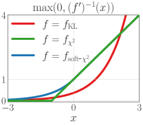
Figure 6: We depict (a) generator functions $f$ of $f$-divergences and (b) corresponding functions $\max(0,(f^{\prime})^{-1}(\cdot))$ used to define the closed-form solution in Proposition 4. While $f_{\mathrm{KL}}(x)$ has a numerical instability for large $x$ and $f_{\chi^{2}}(x)$ provides zero gradients for negative $x$, $f_{\mathrm{soft}\text{-}\chi^{2}}$ does not suffer from both issues.

Pertinent to the result of Proposition 4, one can observe that the choice of the function $f$ of $f$-divergence can affect the numerical stability of optimization especially when using the closed-form solution of $w_{\nu,\lambda}^{*}$:

$$w_{\nu,\lambda}^{*}(s,a)=\max\left(0,(f^{\prime})^{-1}\left(\frac{e_{\nu}(s,a)-\lambda}{\alpha}\right)\right).$$

For example, for the choice of $f(x)=f_{\mathrm{KL}}(x):=x\log x$ that corresponds to KL-divergence, we have $(f_{\mathrm{KL}}^{\prime})^{-1}(x)=\exp(x-1)$. This yields the following closed-form solution of $w_{\nu,\lambda}^{*}$:

$$w_{\nu,\lambda}^{*}(s,a)=\exp\left(\frac{e_{\nu}(s,a)-\lambda}{\alpha}-1\right).$$

However, the choice of $f_{\mathrm{KL}}$ can incur numerical instability due to its inclusion of an $\exp(\cdot)$, i.e. for values of $\frac{1}{\alpha}(e_{\nu}(s,a)-\lambda)$ in order of tens, the value of $w_{\nu,\lambda}^{*}(s,a)$ easily explodes and so does the gradient $\nabla_{\nu}w_{\nu,\lambda}^{*}(s,a)$.

Alternatively, for the choice of $f(x)=f_{\chi^{2}}(x):=\frac{1}{2}(x-1)^{2}$ that corresponds to $\chi^{2}$-divergence, we have $(f_{\chi^{2}}^{\prime})^{-1}(x)=x+1$. This yields the following closed-form solution of $w_{\nu,\lambda}^{*}$:

$$w_{\nu,\lambda}^{*}(s,a)=\mathrm{ReLU}\left(\frac{e_{\nu}(s,a)-\lambda}{\alpha}+1\right),$$

where $\mathrm{ReLU}(x):=\max(0,x)$. Still, this choice may suffer from dying gradient problem: for values of negative $\frac{1}{\alpha}(e_{\nu}(s,a)-\lambda)+1$, the gradient $\nabla_{\nu}w_{\nu,\lambda}^{*}(s,a)$ becomes zero, which can make training $\nu$ slow or even fail.

Consequently, we adopt the function $f=f_{\mathrm{soft}\text{-}\chi^{2}}$ that combines the form of $f_{\mathrm{KL}}$ and $f_{\chi^{2}}$, which can prevent both of the aforementioned issues:

$$f_{\mathrm{soft}\text{-}\chi^{2}}(x):=\begin{cases}x\log x-x+1&\text{if }0<x<1\\ \frac{1}{2}(x-1)^{2}&\text{if }x\geq 1.\end{cases}~{}~{}~{}\Rightarrow~{}~{}~{}(f_{\mathrm{soft}\text{-}\chi^{2}}(x)^{\prime})^{-1}(x)=\begin{cases}\exp(x)&\text{if }x<0\\ x+1&\text{if }x\geq 0\end{cases}$$

This particular choice of $f$ yields the following closed-form solution of $w_{\nu,\lambda}^{*}$:

$$w_{v,\lambda}^{*}(s,a)=\mathrm{ELU}\left(\frac{e_{v}(s,a)-\lambda}{\alpha}\right)+1.$$

Here, $\mathrm{ELU}(x):=\exp(x)-1$ if $x<0$ and $x$ for $x\geq 0$. Note that the solution for $f=f_{\mathrm{soft}\text{-}\chi^{2}}$ is numerically stable for large $\frac{1}{\alpha}(e_{\nu}(s,a)-\lambda)$ and always gives non-zero gradients. We use $f=f_{\mathrm{soft}\text{-}\chi^{2}}$ for the D4RL experiments.

Appendix F Experimental Settings

F.1 Random MDPs

We validate tabular OptiDICE’s efficiency and robustness using randomly generated MDPs with varying numbers of trajectories and the degree of optimality of the data-collection policy, where we follow the experimental protocol of (Laroche et al., 2019; Lee et al., 2020). We conduct repeated experiments for 10,000 runs. For each run, an MDP is generated randomly, and a data-collection policy is constructed according to the given degree of optimality $\zeta\in\{0.9,0.5\}$. Then, $N$ trajectories for $N\in\{10,20,50,100,200,500,1000,2000\}$ are collected using the generated MDP and the data-collection policy $\pi_{\!{}_{D}}$. Finally, the constructed data-collection policy and the collected trajectories are given to each offline RL algorithm, and we measure the mean performance and the CVaR 5% performance.

F.1.1 Random MDP generation

We generate random MDPs with $|S|=50$, $|A|=4$, $\gamma=0.95$, and a deterministic initial state distribution, i.e. $p_{0}(s)=1$ for a fixed $s=s_{0}$. The transition model has connectivity 4: for each $(s,a)$, non-zero probabilities of transition to next states are given to four different states $(s_{1}^{\prime},s_{2}^{\prime},s_{3}^{\prime},s_{4}^{\prime})$, where the random transition probabilities are sampled from a Dirichlet distribution $[p(s_{1}^{\prime}|s,a),p(s_{2}^{\prime}|s,a),p(s_{3}^{\prime}|s,a),p(s_{4}^{\prime}|s,a)]\sim\mathrm{Dir}(1,1,1,1)$. The reward of 1 is given to one state that minimizes the optimal state value at the initial state; other states have zero rewards. This design of the reward function can be understood as we choose a goal state that is the most difficult to reach from the initial state. Once the agent reaches the rewarding goal state, the episode terminates.

F.1.2 Data-collection policy construction

The notion of $\zeta$-optimality of a policy is defined as a relative performance with respect to a uniform random policy $\pi_{\mathrm{unif}}$ and an optimal policy $\pi^{*}$:

$$\text{\big{(}$\zeta$-optimal policy $\pi$'s performance $V^{\pi}(s_{0})$\big{)}}=\zeta V^{*}(s_{0})+(1-\zeta)V^{\pi_{\mathrm{unif}}}(s_{0})$$

However, there are infinitely many ways to construct a $\zeta$-optimal policy. In this work, we follow the way introduced in Laroche et al. (2019) to construct a $\zeta$-optimal data-collection policy, and the process proceeds as follows. First, an optimal policy $\pi^{*}$ and the optimal value function $Q^{*}$ are computed. Then, starting from $\pi_{\mathrm{soft}}:=\pi^{*}$, the policy $\pi_{\mathrm{soft}}$ is softened via $\pi_{\mathrm{soft}}\propto\exp(Q^{*}(s,a)/\tau)$ by increasing the temperature $\tau$ until the performance reaches $\frac{\zeta+1}{2}$-optimality. Finally, the softened policy $\pi_{\mathrm{soft}}$ is perturbed by discounting action selection probability of an optimal action at randomly selected state. This perturbation continues until the performance of the perturbed policy reaches $\zeta$-optimality. The pseudo-code for the process of the data-collection policy construction is presented in Algorithm 3.

Algorithm 3 Data-collection policy construction

  Input: MDP $M$, Degree of optimality of the data-collection policy $\zeta$

  Compute the optimal policy $\pi^{*}$ and its value function $Q^{*}(s,a)$ on the given MDP $M$.

  Initialize $\pi_{\mathrm{soft}}\leftarrow\pi^{*}$

  Initialize a temperature parameter $\tau\leftarrow 10^{-7}$

  while $V^{\pi_{\mathrm{soft}}}(s_{0})>\frac{1}{2}V^{*}(s_{0})+\frac{1}{2}\Big{(}\zeta V^{*}(s_{0})+(1-\zeta)V^{\pi_{\mathrm{unif}}}(s_{0})\Big{)}$ do

     Set $\pi_{\mathrm{soft}}$ to $\pi_{\mathrm{soft}}(a|s)\propto\exp\left(\frac{Q^{*}(s,a)}{\tau}\right)$   $\forall s,a$

     $\tau\leftarrow\tau/0.9$

  end while

  Initialize $\pi_{\!{}_{D}}\leftarrow\pi_{\mathrm{soft}}$

  while $V^{\pi_{\!{}_{D}}}(s_{0})>\zeta V^{*}(s_{0})+(1-\zeta)V^{\pi_{\mathrm{unif}}}(s_{0})$ do

     Sample $s\in S$ uniformly at random.

     $\pi_{\!{}_{D}}(a^{*}|s)\leftarrow 0.9\pi_{\!{}_{D}}(a^{*}|s)$ where $a^{*}=\operatorname*{arg\,max}_{a}Q^{*}(s,a)$.

     Normalize $\pi_{\!{}_{D}}(\cdot|s)$ to ensure $\sum_{a}\pi_{\!{}_{D}}(a|s)=1$.

  end while

  Output: The data-collection policy $\pi_{\!{}_{D}}$

F.1.3 Hyperparameters

We compare our tabular OptiDICE with BasicRL, RaMDP (Petrik et al., 2016), RobustMDP (Nilim & El Ghaoui, 2005; Iyengar, 2005), SPIBB (Laroche et al., 2019), and BOPAH (Lee et al., 2020). For the hyperparameters, we follow the setting in the public code of SPIBB and BOPAH, which are listed as follows:

RaMDP. $\kappa=0.003$ is used for the reward-adjusting hyperparameter.

RobustMDP. $\delta=0.001$ is used for the confidence interval hyperparameter to construct an uncertainty set.

SPIBB. $N_{\wedge}=5$ is used for the data-collection policy bootstrapping threshold.

BOPAH. The 2-fold cross validation criteria and fully state-dependent KL-regularization is used.

OptiDICE. $\alpha=N^{-1}$ for the number $N$ of trajectories is used for the reward-regularization balancing hyperparameter. We also use $f(x)=\frac{1}{2}(x-1)^{2}$ which corresponds to $\chi^{2}$-divergence.

F.2 D4RL benchmark

F.2.1 Task descriptions

We use Maze2D and Gym-MuJoCo environments of D4RL benchmark (Fu et al., 2021) to evaluate OptiDICE and CQL (Kumar et al., 2020) in continuous control tasks. We summarize the descriptions of tasks in D4RL paper (Fu et al., 2021) as follows:

Maze2D. This is a navigation task in 2D state space, while the agent tries to reach a fixed goal location. By using priorly gathered trajectories, the goal of the agent is to find out a shortest path to reach the goal location. The complexity of the maze increases with the order of ”maze2d-umaze”, ”maze2d-medium” and ”maze2d-large”.

Gym-MuJoCo. For each task in $\{$hopper, walker2d, halfcheetah$\}$ of MuJoCo continuous controls, the dataset is gathered in the following ways.

random. The dataset is generated by a randomly initialized policy in each task.

medium. The dataset is generated by using the policy trained by SAC (Haarnoja et al., 2018) with early stopping.

medium-replay. The “replay” dataset consists of the samples gathered during training the policy for “medium” dataset. The “medium-replay” dataset includes both “medium” and “replay” datasets.

medium-expert. The dataset is given by using the same amount of expert trajectories and suboptimal trajectories, where those suboptimal ones are gathered by using either a randomly uniform policy or a medium-performance policy.

F.2.2 Hyperparameter settings for CQL

We follow the hyperparameters specified by Kumar et al. (2020). For learning both the Q-funtions and the policy, fully-connected multi-layer perceptrons (MLPs) with three hidden layers and ReLU activations are used, where the number of hidden units on each layer is equal to 256. A Q-function learning rate of 0.0003 and a policy learning rate of 0.0001 are used with Adam optimizer for these networks. CQL$(\mathcal{H})$ is evaluated, with an approximate max-backup (see Appendix F of (Kumar et al., 2020) for more details) and a static $\alpha=5.0$, which controls the conservativeness of CQL. The policy of CQL is updated for 2,500,000 iterations, while we use 40,000 warm-up iterations where we update Q-functions as usual, but the policy is updated according to the behavior cloning objective.

F.2.3 Hyperparameter settings for OptiDICE

For neural networks $\nu_{\theta},e_{\phi},\pi_{\psi}$ and $\pi_{\beta}$ in Algorithm 1, we use fully-connected MLPs with two hidden layers and ReLU activations, where the number of hidden units on each layer is equal to 256. For $\pi_{\psi}$, we use tanh-squashed normal distribution. We regularize the entropy of $\pi_{\psi}$ with learnable entropy regularization coefficients, where target entropies are set to be the same as those in SAC (Haarnoja et al., 2018) ($-\mathrm{dim}(A)$ for each task). For $\pi_{\beta}$, we use tanh-squashed mixture of normal distributions, where we build means and standard deviations of each mixture component upon shared hidden outputs. No entropy regularization is applied to $\pi_{\beta}$. For both $\pi_{\psi}$ and $\pi_{\beta}$, means are clipped within $(-7.24,7.24)$, while log of standard deviations are clipped within $(-5,2)$. For the optimization of each network, we use stochastic gradient descent with Adam optimizer and its learning rate $0.0003$. The batch size is set to be $512$. Before training neural networks, we preprocess the dataset $D$ by standardizing observations and rewards. We additionally scale the rewards by multiplying 0.1. We update the policy $\pi_{\psi}$ for 2,500,000 iterations, while we use 500,000 warm-up iterations for other networks, i.e., those networks other than $\pi_{\psi}$ are updated for 3,000,000 iterations.

For each task and OptiDICE methods (OptiDICE-minimax, OptiDICE-MSE), we search the number $K$ of mixtures (for $\pi_{\beta}$) within $\{1,5,9\}$ and the coefficient $\alpha$ within $\{0.0001,0.001,0.01,0.1,1\}$, while we additionally search $\alpha$ over $\{2,5,10\}$ for hopper-medium-replay. The hyperparameters $K$ and $\alpha$ showing the best mean performance were chosen, which are described as follows:

Table 2: Hyperaparameters

Task	OptiDICE-MSE		OptiDICE-minimax
	$K$	$\alpha$	$K$	$\alpha$
maze2d-umaze	5	0.001	1	0.01
maze2d-medium	5	0.0001	1	0.01
maze2d-large	1	0.01	1	0.01
hopper-random	5	1	5	1
hopper-medium	9	0.1	9	0.1
hopper-medium-replay	9	10	1	2
hopper-medium-expert	9	1	5	1
walker2d-random	9	0.0001	1	0.0001
walker2d-medium	9	0.01	5	0.01
walker2d-medium-replay	9	0.1	9	0.1
walker2d-medium-expert	5	0.01	5	0.01
halfcheetah-random	5	0.0001	9	0.001
halfcheetah-medium	1	0.01	1	0.1
halfcheetah-medium-replay	9	0.01	1	0.1
halfcheetah-medium-expert	9	0.01	9	0.01

Appendix G Experimental results

G.1 Experimental results for $\gamma=0.99$

Table 3: Normalized performance of OptiDICE compared with baselines. Mean scores for baselines—BEAR (Kumar et al., 2019), BRAC (Wu et al., 2019), AlgaeDICE (Nachum et al., 2019b), and CQL (Kumar et al., 2020)— come from D4RL benchmark. We also report the performance of CQL (Kumar et al., 2020) obtained by running the code released by authors (denoted as CQL (ours) in the table). OptiDICE achieves the best performance on 6 tasks compared to our baselines. Note that 3-run mean scores without confidence intervals were reported on each task by Fu et al. (2021). For CQL (ours) and OptiDICE, we use 5 runs and report means and 95% confidence intervals.

Task	BC	SAC	BEAR	BRAC -v	Algae DICE	CQL	CQL (ours)	OptiDICE
								minimax	MSE
maze2d-umaze	3.8	88.2	3.4	-16.0	-15.7	5.7	-14.9 $\pm$ 0.7	111.0 $\pm$ 8.3	105.8 $\pm$ 17.5
maze2d-medium	30.3	26.1	29.0	33.8	10.0	5.0	17.2 $\pm$ 8.7	109.9 $\pm$ 7.7	145.2 $\pm$ 17.5
maze2d-large	5.0	-1.9	4.6	40.6	-0.1	12.5	1.6 $\pm$ 3.8	116.1 $\pm$ 43.1	155.7 $\pm$ 33.4
hopper-random	9.8	11.3	11.4	12.2	0.9	10.8	10.7 $\pm$ 0.0	11.2 $\pm$ 0.1	10.7 $\pm$ 0.2
hopper-medium	29.0	0.8	52.1	31.1	1.2	58.0	89.8 $\pm$ 7.6	92.9 $\pm$ 2.6	94.1 $\pm$ 3.7
hopper-medium-replay	11.8	3.5	33.7	0.6	1.1	48.6	33.3 $\pm$ 2.2	36.4 $\pm$ 1.1	30.7 $\pm$ 1.2
hopper-medium-expert	111.9	1.6	96.3	0.8	1.1	98.7	112.3 $\pm$ 0.2	111.5 $\pm$ 0.6	106.7 $\pm$ 1.8
walker2d-random	1.6	4.1	7.3	1.9	0.5	7.0	3.0 $\pm$ 1.8	9.4 $\pm$ 2.2	9.9 $\pm$ 4.3
walker2d-medium	6.6	0.9	59.1	81.1	0.3	79.2	73.7 $\pm$ 2.7	21.8 $\pm$ 7.1	20.8 $\pm$ 3.1
walker2d-medium-replay	11.3	1.9	19.2	0.9	0.6	26.7	13.4 $\pm$ 0.8	21.5 $\pm$ 2.9	21.6 $\pm$ 2.1
walker2d-medium-expert	6.4	-0.1	40.1	81.6	0.4	111.0	99.7 $\pm$ 7.2	74.7 $\pm$ 7.5	74.8 $\pm$ 9.2
halfcheetah-random	2.1	30.5	25.1	31.2	-0.3	35.4	25.5 $\pm$ 0.5	8.3 $\pm$ 0.8	11.6 $\pm$ 1.2
halfcheetah-medium	36.1	-4.3	41.7	46.3	-2.2	44.4	42.3 $\pm$ 0.1	37.1 $\pm$ 0.1	38.2 $\pm$ 0.1
halfcheetah-medium-replay	38.4	-2.4	38.6	47.7	-2.1	46.2	43.1 $\pm$ 0.7	38.9 $\pm$ 0.5	39.8 $\pm$ 0.3
halfcheetah-medium-expert	35.8	1.8	53.4	41.9	-0.8	62.4	53.5 $\pm$ 13.3	76.2 $\pm$ 7.0	91.1 $\pm$ 3.7

G.2 Experimental results with importance-weighted BC

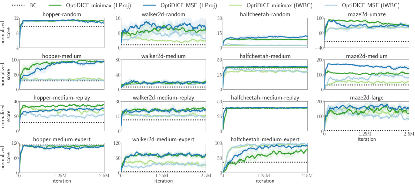
Figure 7: Performance of BC, OptiDICE with importance-weighted BC (IWBC) and information projection (I-Proj) methods on D4RL benchmark. $\gamma=0.99$ is used.

The empirical results of OptiDICE for different policy extraction methods (information-weighted BC, I-projection methods) are depicted in Figure 7. For those results with IWBC, we search $\alpha$ within $\{0.0001,0.001,0.01,0.1,1\}$ and choose one with the best mean performance, which are summarized in Table 4. The hyperparameters other than $\alpha$ are the same as those used for information-projection methods, which is described in Section F.2.3. We empirically observe that policy extraction with information projection method performs better than the extraction with importance-weighted BC, as discussed in Section 3.3.

Table 4: Hyperaparameters for importance-weighted BC

Task	OptiDICE-MSE	OptiDICE-minimax
	$\alpha$	$\alpha$
maze2d-umaze	0.001	0.001
maze2d-medium	0.0001	0.001
maze2d-large	0.001	0.001
hopper-random	1	1
hopper-medium	0.01	0.1
hopper-medium-replay	0.1	0.1
hopper-medium-expert	0.1	0.1
walker2d-random	0.0001	0.0001
walker2d-medium	0.1	0.1
walker2d-medium-replay	0.1	0.1
walker2d-medium-expert	0.01	0.01
halfcheetah-random	0.001	0.01
halfcheetah-medium	0.0001	0.1
halfcheetah-medium-replay	0.01	0.01
halfcheetah-medium-expert	0.01	0.01

G.3 Experimental results for $\gamma\in\{0.99,0.999,0.9999,1.0\}$

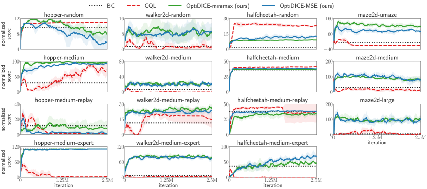
Figure 8: Performance of BC, CQL, OptiDICE-minimax and OptiDICE-MSE on D4RL benchmark for $\gamma=0.99$.

Figure 9: Performance of BC, CQL, OptiDICE-minimax and OptiDICE-MSE on D4RL benchmark for $\gamma=0.999$.

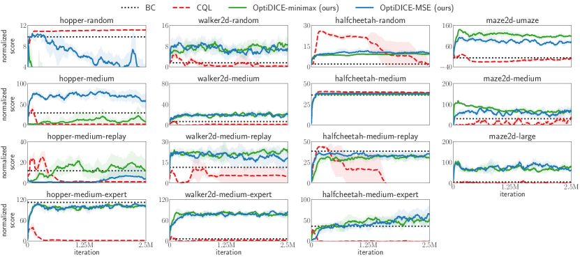
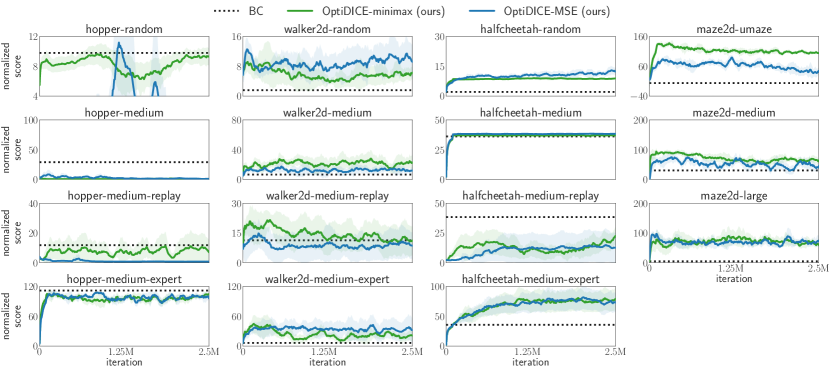
Figure 10: Performance of BC, CQL, OptiDICE-minimax and OptiDICE-MSE on D4RL benchmark for $\gamma=0.9999$.

Figure 11: Performance of BC, OptiDICE-minimax and OptiDICE-MSE on D4RL benchmark for $\gamma=1$. Note that CQL cannot deal with $\gamma=1$ case. Thus, we only provide the results of OptiDICE and BC.

References

• Agarwal et al. (2020) Agarwal, R., Schuurmans, D., and Norouzi, M. An optimistic perspective on offline reinforcement learning. In Proceedings of the 37th International Conference on Machine Learning (ICML), 2020.
• Baird (1995) Baird, L. Residual algorithms: Reinforcement learning with function approximation. In Proceedings of the 12th International Conference on Machine Learning (ICML), 1995.
• Boyd et al. (2004) Boyd, S., Boyd, S. P., and Vandenberghe, L. Convex optimization. Cambridge university press, 2004.
• Dai et al. (2020) Dai, B., Nachum, O., Chow, Y., Li, L., Szepesvari, C., and Schuurmans, D. CoinDICE: Off-policy confidence interval estimation. In Advances in Neural Information Processing Systems (NeurIPS), 2020.
• Deng et al. (2009) Deng, J., Dong, W., Socher, R., Li, L.-J., Li, K., and Fei-Fei, L. ImageNet: A large-scale hierarchical image database. In Proceedings of IEEE Conference on Computer Vision and Pattern Recognition (CVPR), 2009.
• Devlin et al. (2019) Devlin, J., Chang, M.-W., Lee, K., and Toutanova, K. BERT: Pre-training of deep bidirectional transformers for language understanding. In Proceedings of the 2019 Conference of the North American Chapter of the Association for Computational Linguistics: Human Language Technologies, Volume 1 (Long and Short Papers), 2019.
• Ernst et al. (2005) Ernst, D., Geurts, P., and Wehenkel, L. Tree-based batch mode reinforcement learning. Journal of Machine Learning Research (JMLR), 2005.
• Fox et al. (2016) Fox, R., Pakman, A., and Tishby, N. Taming the noise in reinforcement learning via soft updates. In Proceedings of the 32nd Conference on Uncertainty in Artificial Intelligence (UAI), 2016.
• Fu et al. (2021) Fu, J., Kumar, A., Nachum, O., Tucker, G., and Levine, S. D4RL: Datasets for deep data-driven reinforcement learning, 2021. URL https://openreview.net/forum?id=px0-N3_KjA.
• Fujimoto et al. (2018) Fujimoto, S., van Hoof, H., and Meger, D. Addressing function approximation error in actor-critic methods. In Proceedings of the 35th International Conference on Machine Learning (ICML), 2018.
• Fujimoto et al. (2019) Fujimoto, S., Meger, D., and Precup, D. Off-policy deep reinforcement learning without exploration. In Proceedings of the 36th International Conference on Machine Learning (ICML), 2019.
• Goodfellow et al. (2014) Goodfellow, I. J., Pouget-Abadie, J., Mirza, M., Xu, B., Warde-Farley, D., Ozair, S., Courville, A., and Bengio, Y. Generative adversarial networks. In Advances in Neural Information Processing Systems (NeurIPS), pp.  2672–2680, 2014.
• Haarnoja et al. (2018) Haarnoja, T., Zhou, A., Abbeel, P., and Levine, S. Soft actor-critic: Off-policy maximum entropy deep reinforcement learning with a stochastic actor. In Proceedings of the 35th International Conference on Machine Learning (ICML), 2018.
• Iyengar (2005) Iyengar, G. N. Robust dynamic programming. Mathematics of Operations Research, 2005.
• Jaques et al. (2019) Jaques, N., Ghandeharioun, A., Shen, J. H., Ferguson, C., Lapedriza, A., Jones, N., Gu, S., and Picard, R. Way off-policy batch deep reinforcement learning of implicit human preferences in dialog, 2019.
• Kidambi et al. (2020) Kidambi, R., Rajeswaran, A., Netrapalli, P., and Joachims, T. MOReL : Model-based offline reinforcement learning. In Advances in Neural Information Processing Systems (NeurIPS), 2020.
• Kostrikov et al. (2019a) Kostrikov, I., Agrawal, K. K., Dwibedi, D., Levine, S., and Tompson, J. Discriminator-Actor-Critic: Addressing sample inefficiency and reward bias in adversarial imitation learning. In Proceedings of the 7th International Conference on Learning Representations (ICLR), 2019a.
• Kostrikov et al. (2019b) Kostrikov, I., Nachum, O., and Tompson, J. Imitation learning via off-policy distribution matching. In Proceedings of the 7th International Conference on Learning Representations (ICLR), 2019b.
• Krizhevsky et al. (2012) Krizhevsky, A., Sutskever, I., and Hinton, G. E. ImageNet classification with deep convolutional neural networks. In Advances in Neural Information Processing Systems (NeurIPS), 2012.
• Kumar et al. (2019) Kumar, A., Fu, J., Soh, M., Tucker, G., and Levine, S. Stabilizing off-policy Q-learning via bootstrapping error reduction. In Advances in Neural Information Processing Systems (NeurIPS), 2019.
• Kumar et al. (2020) Kumar, A., Zhou, A., Tucker, G., and Levine, S. Conservative Q-learning for offline reinforcement learning. In Advances in Neural Information Processing Systems (NeurIPS), 2020.
• Lange et al. (2012) Lange, S., Gabel, T., and Riedmiller, M. Reinforcement learning: State-of-the-art. Springer Berlin Heidelberg, 2012.
• Laroche et al. (2019) Laroche, R., Trichelair, P., and Des Combes, R. T. Safe policy improvement with baseline bootstrapping. In Proceedings of the 36th International Conference on Machine Learning (ICML), 2019.
• Lee et al. (2020) Lee, B.-J., Lee, J., Vrancx, P., Kim, D., and Kim, K.-E. Batch reinforcement learning with hyperparameter gradients. In Proceedings of the 37th International Conference on Machine Learning (ICML), 2020.
• Levine et al. (2020) Levine, S., Kumar, A., Tucker, G., and Fu, J. Offline reinforcement learning: Tutorial, review, and perspectives on open problems, 2020.
• Lillicrap et al. (2016) Lillicrap, T. P., Hunt, J. J., Pritzel, A., Heess, N., Erez, T., Tassa, Y., Silver, D., and Wierstra, D. Continuous control with deep reinforcement learning. In Proceedings of the 4th International Conference on Learning Representations (ICLR), 2016.
• Nachum et al. (2019a) Nachum, O., Chow, Y., Dai, B., and Li, L. DualDICE: Behavior-agnostic estimation of discounted stationary distribution corrections. In Advances in Neural Information Processing Systems (NeurIPS), 2019a.
• Nachum et al. (2019b) Nachum, O., Dai, B., Kostrikov, I., Chow, Y., Li, L., and Schuurmans, D. AlgaeDICE: Policy gradient from arbitrary experience. arXiv preprint arXiv:1912.02074, 2019b.
• Nilim & El Ghaoui (2005) Nilim, A. and El Ghaoui, L. Robust control of markov decision processes with uncertain transition matrices. Operations Research, 2005.
• Peng et al. (2019) Peng, X. B., Kumar, A., Zhang, G., and Levine, S. Advantage-weighted regression: Simple and scalable off-policy reinforcement learning, 2019.
• Petrik et al. (2016) Petrik, M., Ghavamzadeh, M., and Chow, Y. Safe policy improvement by minimizing robust baseline regret. In Advances in Neural Information Processing Systems (NeurIPS), 2016.
• Puterman (1994) Puterman, M. L. Markov decision processes: Discrete stochastic dynamic programming. John Wiley & Sons, Inc., 1st edition, 1994.
• Schulman et al. (2017) Schulman, J., Chen, X., and Abbeel, P. Equivalence between policy gradients and soft Q-learning, 2017.
• Sutton & Barto (1998) Sutton, R. S. and Barto, A. G. Reinforcement learning: An introduction. MIT Press, 1998.
• Sutton et al. (1999) Sutton, R. S., Precup, D., and Singh, S. Between MDPs and semi-MDPs: A framework for temporal abstraction in reinforcement learning. Artificial Intelligence, 1999.
• Szita & Lörincz (2008) Szita, I. and Lörincz, A. The many faces of optimism: A unifying approach. In Proceedings of the 25th International Conference on Machine Learning (ICML), 2008.
• Wu et al. (2019) Wu, Y., Tucker, G., and Nachum, O. Behavior regularized offline reinforcement learning, 2019.
• Yang et al. (2020) Yang, M., Nachum, O., Dai, B., Li, L., and Schuurmans, D. Off-policy evaluation via the regularized lagrangian. In Advances in Neural Information Processing Systems (NeurIPS), 2020.
• Yu et al. (2020a) Yu, C., Liu, J., and Nemati, S. Reinforcement learning in healthcare: A survey, 2020a.
• Yu et al. (2020b) Yu, F., Chen, H., Wang, X., Xian, W., Chen, Y., Liu, F., Madhavan, V., and Darrell, T. BDD100K: A diverse driving dataset for heterogeneous multitask learning. Proceedings of IEEE Conference on Computer Vision and Pattern Recognition (CVPR), 2020b.
• Yu et al. (2020c) Yu, T., Thomas, G., Yu, L., Ermon, S., Zou, J., Levine, S., Finn, C., and Ma, T. MOPO: Model-based offline policy optimization. In Advances in Neural Information Processing Systems (NeurIPS), 2020c.
• Zhang et al. (2020a) Zhang, R., Dai, B., Li, L., and Schuurmans, D. GenDICE: Generalized offline estimation of stationary values. In Proceedings of the 8th International Conference on Learning Representations (ICLR), 2020a.
• Zhang et al. (2020b) Zhang, S., Liu, B., and Whiteson, S. GradientDICE: Rethinking generalized offline estimation of stationary values. In Proceedings of the 35th International Conference on Machine Learning (ICML), 2020b.