Covariance Matching based robust Adaptive Cubature Kalman Filter

Abstract

This letter explores covariance matching based adaptive robust cubature Kalman filter (CMRACKF). In this method, the innovation sequence is used to determine the covariance matrix of measurement noise that can overcome the limitation of conventional CKF. In the proposed algorithm, weights are adaptively adjust and used for updating the measurement noise covariance matrices online. It can also enhance the adaptive capability of the ACKF. The simulation results are illustrated to evaluate the performance of the proposed algorithm.

Robust Adaptive Cubature Kalman, window method, target tracking, covariance matching.

1 Introduction

Kalman filter (KF) has been widely used state estimator in several fields; in navigation, target tracking [1], robotics, control and signal processing[2]. In practice, the system and measurement model of the KF are not known exactly. Moreover, the system becomes nonlinear and their noise models are vary with time [1]. Over years, several variants of non-linear estimation methods; extended KF (EKF), Unscented Kalman filter (UKF), and cubature Kalman filter (CKF) have been developed for estimating state of a nonlinear system [3, 4]. The EKF performance is limited by the calculation of Jacobin errors. To improve the performance and by addressing the EKF drawback, UKF has been developed based on Unscented Transform [3]. In the UKF, a set of sigma points has used to approximate the mean and covariance of the state vectors. However, the accuracy of UKF has limited for higher order system [5, 2]. CKF has been proposed to eliminate the limitation of UKF and used for solving the higher order systems. The CKF has developed by set of cubature points and used to approximate the state vector in terms of posteriori mean and covariance. The CKF and UKF have the same accuracy, however better than the EKF filter [4].

In the CKF, a priori knowledge of the system and noise models are usually unknown in real-time then CKF becomes sub-optimal. Moreover, the uncertainties in the system and measurement models may leads to large errors. Hence, CKF shows divergence behaviour under these conditions [6]. Recent past, many authors have been focusing on adaptive CKF and being addressed limitation on CKF that can applied in nonlinear system analysis with additive Gaussian noise [5]. The innovation or residual based adaptive methods have been developed and followed by using covariance matching, Bayesian approach, multiple model estimation (MME) and Maximum likelihood method [7]. In covariance matching based AKF [7], in which window average method is used to estimate the noise covariances matrices [8]. However, for improving the practicality of the adaptive CKF, robust methods are better by adaptively updating the noise statistics online [9, 10].

To the best of authors knowledge’s, there is a limited work on robust adaptive cubature Kalman filter. This letter presents an improved covariance matching based robust adaptive cubature Kalman filter (CMRACKF) for addressing the outliers in the measurements. In the proposed algorithm, moving average method (MAM) is used to adapt the noise statistics of innovation vector and the weights on each window are adjusted. The ability of the CMRACKF algorithm is to estimate and update the noise statistics online.

The rest of the paper was organized as follows; The description of the traditional Cubature Kalman filter algorithm is presented in Section II. Section III provides the briefly on ACKF algorithm and then the proposed CMRACKF algorithm in Section IV. Simulation examples along with performance analysis of the proposed algorithm is given in Section IV. Section V presents the conclusions of the paper.

2 Cubature Kalman filtering

In nonlinear state estimation, Cubature Kalman Filter (CKF) is the better method has been widely used algorithm for solving the higher dimensions of the stochastic systems. In the CKF, cubature points are required to approximate the state vector mean and error covariance followed by the spherical radial cubature criterion [4].

Let us consider a discrete time stochastic nonlinear dynamic system and measurement equations:

$${\bf x_{k}}={\bf f({x_{k-1}},u_{k-1})}+{\bf w_{k-1}}$$ (1)

$${\bf z}_{k}={\bf h({\bf x_{k}})}+{\bf v_{k}}$$ (2)

where, $\bf x_{k}\in R^{n}$ is the state vector, ${\bf u_{k}}\bf\in R^{r}$ is the input vector, ${\bf z_{k}}\bf\in R^{m}$ is the measurement vector at time ${k}$. ${\bf f({x}_{k-1})},{\bf h({k})}$ are the nonlinear system dynamic and measurement functions. The process and measurement noise are assumed to be white Gaussian noise with zero mean and finite variance, represented as ${\bf w_{k}}=N(0,{\bf Q_{k}})$ and ${\bf v_{k}}=N(0,{\bf R_{k}})$, respectively. The step-wise implementation of CKF algorithm is follows [4]

The detailed algorithm of the CKF is given as follows.
Step 1: Initialize the state estimation ${\bf\hat{x}}_{0}$ and error covariance matrix ${\bf\hat{P}}_{0}$ as

$$\begin{cases}{\bf\hat{x}_{0}}=E[{\bf x_{0}}]\\ {\bf\hat{P}_{0}}=E[({\bf x_{0}}-{\bf\hat{x}_{0}})({\bf x_{0}}-{\bf\hat{x}_{0}})^{T}]\end{cases}$$ (3)

A set of 2L cubature points are given by set $[{({\bf\chi_{k}})_{i}}\quad{W_{i}}^{m}]$, where ${({\bf\chi_{k}})_{i}}$ is the i-th cubature point and corresponding weights are represented as

$${{\bf\chi}_{i}} =\sqrt{\bf L}[1]_{i},$$ (4)

$${\bf W_{i}}^{m} =\frac{1}{2L}, i=1,2..2L$$

where, [1](i) denotes its i-th column vector of the the identity matrix. The steps involved in the predicted (time-update) and the measurement-update of the CKF are summarised in below.

Prediction:
(1) factorise and evaluate the cubature points:

$${\bf\hat{P}_{k-1}} =S_{k-1}S_{k-1}^{T},$$ (5)

$${({\bf\chi_{k}})_{i}} =S_{k}{{\bf\xi}_{i}}+{\bf\hat{x}_{k}}, i=1,2..2L$$

(2) Propagate each sigma points through the nonlinear system as

$${({\bf X_{k-1}})_{i}}={\bf f}({{({\bf\chi_{k}})_{i}},\bf u_{k}}),\quad i=1,2......2L$$ (6)

(3) Evaluate the predicted state ${\bf\hat{x}_{k}}^{-}$ and state error covariance ${\bf\hat{P}_{k}}^{-}$ based on the transformed sigma points as

$${\bf\hat{x}_{k-1}}^{-} =\frac{1}{2L}\sum\limits_{i=1}^{2L}{({\bf X_{k-1}})_{i}},$$ (7)

$${\bf\hat{P}_{k-1}}^{-} =\frac{1}{2L}\sum\limits_{i=1}^{2L}{({\bf X_{k-1}})_{i}}{({\bf X_{k-1}})_{i}^{\top}}-{\bf\hat{x}_{k-1}}{\bf\hat{x}_{k-1}}^{{-}^{\top}}+{\bf Q_{k-1}}$$

Measurement update:
(1) factorise and evaluate the new cubature points:

$${\bf\hat{P}_{k-1}} =S_{k-1}S_{k-1}^{T},$$ (8)

$${({\bf Z_{k-1}})_{i}} =S_{k-1}{{\bf\xi}_{i}}+{\bf\hat{x}_{k-1}}, i=1,2..2L$$

(2) Propagate new sigma points through the nonlinear system as

$${({\bf z_{k-1}})_{i}}={\bf h}({{({\bf Z_{k-1}})_{i}}}),\quad i=1,2......2L$$ (9)

(3) Evaluate the predicted measurements ${\bf\hat{z}_{k}}^{-}$ based on the new sigma points as

$${\bf\hat{z}_{k-1}}^{-} =\frac{1}{2L}\sum\limits_{i=1}^{2L}{({\bf Z_{k-1}})_{i}},$$ (10)

(4) calculate the the cross and auto covariance of state and measurement values of ${\bf P_{xz,k}}$ and ${\bf P_{zz,k}}$ are

$${\bf P_{xz,k-1}} =\frac{1}{2L}\sum\limits_{i=1}^{2L}{({\bf X_{k}})_{i}}{({\bf Z_{k}})_{i}^{\top}}-{\bf\hat{x}_{k-1}}^{-}{\bf\hat{z}_{k-1}}^{{-}^{\top}}$$ (11)

$${\bf P_{zz,k-1}} =\sum\limits_{i=1}^{2L}{({\bf Z_{k-1}})_{i}}{({\bf Z_{k-1}})_{i}^{\top}}-{\bf\hat{z}_{k-1}}^{-}{\bf\hat{z}_{k-1}}^{{-}^{\top}}+{\bf R_{k-1}}$$

(5) evaluate the Kalman gain and the updated stat and error covariance are

$${\bf K_{k}} ={\bf P_{xz,k-1}}{\bf P_{zz,k-1}^{-1}},$$ (12)

$${\bf\hat{x}_{k}} ={\bf\hat{x}_{k-1}^{-}}+{\bf K_{k}}({\bf z_{k}}-{\bf\hat{z}_{k-1}^{-}})$$

$${\bf\hat{P}_{k}} ={\bf\hat{P}_{k-1}}^{-}-{\bf K_{k}}{\bf P_{zz,k-1}}{\bf K_{k}}^{\top}.$$

where, (${\bf\upsilon_{k}}={\bf z_{k}}-{\bf\hat{z}_{k-1}^{-}}$) is the innovation sequence. ${\bf\hat{P}_{k}}$, is the posterior state estimate of state. More detailed explanation of CKF can be found in [4]

3 Adaptive Cubature Kalman Filter

To improve the optimality and solving divergence issue of CKF, adaptive Kalman filters [7] have been developed for updating the ${\bf Q_{k}}$ and ${\bf R_{k}}$ online. An innovation based adaptive estimation (IAE) ACKF is the one widely used estimation method [6].

3.1 Innovation based adaptive estimation Adaptive cubature Kalman filtering (IAE-ACKF)

To address the CKF limitation and solving the divergence solution, the ACKF has briefly presented [8, 10]. In the ACKF, the innovation sequence (${\bf\upsilon_{k}}={\bf z_{k}}-{\bf h}{\bf\hat{x}^{-}_{k}}$) is calculated between measured and predicted measurements difference. By taking covariance, i.e., $E({\bf\upsilon_{k}}{\bf\upsilon_{k}^{\top}})$, then theoretical covariance matrix of ${\bf C_{\upsilon k}}$ is

$${\bf C_{\upsilon k}}={\bf h}{\bf\hat{P}^{-}_{k}}{\bf h^{T}}+{\bf{R}_{k}}$$ (13)

The window average method and followed by the covariance matching principle in ACKF [7], is used to estimate the covariance matrix of innovation sequence as

$${\bf\hat{C}_{\upsilon k}}=\frac{1}{N_{w}}\sum_{j=j0}^{k}{\bf\upsilon_{j}}{\bf\upsilon_{j}}^{T}$$ (14)

where, $j_{0}={k}-{N_{w}}+1$ is the first epoch. ${\bf\upsilon_{j}}$ and ${N_{w}}$ are the innovation sequence and window size respectively. If the window size is too small, the estimation of measurement noise covariance can be noisy [5].

4 Proposed algorithm: CMRACKF

In the proposed method, the measurement noise covariance is matrix is estimated; (i) covariance matching principle (ii) estimated measurements variance (see in equation (16)). At each epoch, the individual weights contribution to data samples of measurements and state estimator calculation by the estimated variance of measurements. In the CMRACKF, an adaptive tuning parameter also is used to control the disturbances due to the effect of the residual error measurements.

4.0.1 Adaption of measurement noise covariance matrix

In the CMRACKF algorithm, the estimated measurement noise covariance matrix (${\bf\hat{R}_{k}}$) is updated according to the innovation sequence as

$${\bf\hat{R}}_{k-j}^{*}=\frac{1}{N_{w}}\sum_{j=j0}^{k}{\omega({\bf\sigma^{2}_{k-j}})}{\bf\upsilon_{j}}{\bf\upsilon_{j}}^{T}-{\bf h}{\bf\hat{P}_{k}^{-}}{\bf h}^{T}$$ (15)

where, ${\omega({\bf\hat{\sigma}^{2}_{k-j}})}$ is the weighted function of the measurement error is calculated as follows;

4.0.2 Calculation of Weight

The estimated variance and corresponding weights of measurement are defined as [10]

$${\bf\hat{\sigma}^{2}_{k-j}} =\frac{{\bf\upsilon_{k}^{T}{\bf R_{k}{\bf\upsilon_{k}}}}}{\bf r_{k}},$$ (16)

$${\bf\omega({\bf\hat{\sigma}^{2}_{k-j}})} =\frac{(\frac{1}{{\bf\hat{\sigma}^{2}_{k-j}}})}{({\sum_{j=1}^{N_{w}}{\frac{1}{{\bf\hat{\sigma}^{2}_{k-j}}}}})}$$

subject to the sum of the weights are equal to 1, i.e; $\sum_{j=1}^{N_{w}}{\bf\omega({\bf\hat{\sigma}^{2}_{k-j}})}=1$. Where, ${\bf r_{k}}$ denotes the number of measurements at each epoch $k$ [6]. In the CMRACKF algorithm, the estimated covariance of innovation sequence is updated by

$${\bf\hat{C}_{\bf\upsilon k}}=\frac{1}{N_{w}}\sum_{j=j0}^{k}{\omega({\hat{\sigma}^{2}_{k-j}})}{\bf\upsilon_{j}}{\bf\upsilon_{j}^{\top}}$$ (17)

where ${\omega(.)}$, $\bf\upsilon_{j}$ and ${\bf\hat{C}_{\bf\upsilon k}}$ are weight function, innovation sequence and its covariance matrix, respectively.

Theorem 1.

Suppose the measurement and system noise statistics are two noise control parameters are very small in considered window size of ${N_{w}}$. Then, a novel noise statistic estimator can be developed and derived as

$${\bf\hat{R}_{k-j}^{*}}=\frac{1}{N_{w}}\sum\limits_{j=0}{{}^{N}}{\omega({\bf\sigma^{2}_{k-j}})}{\bf\upsilon_{j}}{\bf\upsilon_{j}^{\top}}-{\bf h_{k-j}}{\bf\hat{P}_{k-j}}{\bf h_{k-j}^{\top}}$$ (18)

$${\bf\hat{Q}}_{k-j}^{*}=\frac{1}{{N_{w}}}[\sum\limits_{j=0}^{N}{\omega({\bf\sigma^{2}_{k-j}})}{\bf\upsilon_{j}}{\bf\upsilon_{j}}^{\top}+\sum\limits_{j=0}^{N}{\omega({\bf\sigma^{2}_{k-j}})}{\bf\eta_{j}}{\bf\eta_{j}}^{\top}]$$ (19)

$$-{\bf h_{k-j}}[\frac{1}{2L}\sum\limits_{i=1}^{2L}{({\bf X_{k-1}})_{i}}{({\bf X_{k-1}})_{i}^{\top}}-{\bf\hat{x}_{k-1}}{\bf\hat{x}_{k-1}}^{{-}^{\top}}+{\bf\hat{P}_{k-j}}]{\bf h_{k-j}^{\top}}$$

Proof.

Let us assume that the window width is ${N_{w}}$ and there are ${N_{w}}$ measurements within $t_{k-N}$ to $t_{k}$. Suppose the measurement noise statistics is very small variations within window width. The innovation is described as

$${\bf\upsilon_{k}}={\bf z_{k}}-{\bf\hat{z}_{k}^{-}}$$ (20)

and substituting the measurement equation in (2) into (21), we have

$${\bf\upsilon_{k}}={\bf h(.)}({\bf{x}_{k}}-{\bf\hat{x}^{-}_{k}})+{\bf v_{k}}$$ (21)

Define the predicted and estimated state error are

$${\bf\Delta\hat{x}^{-}_{k}} ={\bf{x}_{k}}-{\bf\hat{x}^{-}_{k}},{\bf\hat{P}_{k}^{-}}=E[{\bf\Delta\hat{x}^{-}_{k}}{\bf\Delta\hat{x}^{-}_{k}}^{\top}]$$ (22)

$${\bf\Delta\hat{x}_{k}} ={\bf{x}_{k}}-{\bf\hat{x}_{k}},{\bf\hat{P}_{k}}=E[{\bf\Delta\hat{x}_{k}}{\bf\Delta\hat{x}_{k}}^{\top}]$$

By taking the sample mean and the covariances for a limited number of sample of the innovation sequence is

$${\bf\bar{\upsilon}_{k}} =\frac{1}{{N_{w}}}\sum\limits_{j=1}^{{N_{w}}}{\bf\upsilon_{k-j}},$$ (23)

$$E[{\bf\upsilon_{k}}{\bf\upsilon_{k}}^{\top}] =\frac{1}{{N_{w}}-1}\sum\limits_{j=1}^{{N_{w}}}{\bf\omega({\bf\hat{\sigma}^{2}_{k-j}})}({\bf\upsilon_{k-j}}-{\bf\bar{\upsilon}_{k}})({\bf\upsilon_{k-j}}-{\bf\bar{\upsilon}_{k}}^{\top})$$

From equation (22), we can apply the weighted sample covariances

$$E[{\bf\upsilon_{k}}{\bf\upsilon_{k}}^{\top}] =E[{\bf h}({\bf{x}_{k}}-{\bf\hat{x}^{-}_{k}})+{\bf v_{k}}][{\bf h}({\bf{x}_{k}}-{\bf\hat{x}^{-}_{k}})+{\bf v_{k}})]^{\top}$$ (24)

$$=E[{\bf h}({\bf\Delta\hat{x}^{-}_{k}})+{\bf v_{k}}][{\bf h}({\bf\Delta\hat{x}^{-}_{k}})+{\bf v_{k}})]^{\top}$$

$$={\bf h}E[({\bf\Delta\hat{x}^{-}_{k}})({\bf\Delta\hat{x}^{-}_{k}})^{\top}]{\bf h^{\top}}+E[{\bf v_{k}}{\bf v}^{\top}_{k}]$$

$$={\bf h}{\bf\hat{P}_{k}}{\bf h^{\top}}+{\bf R_{k}}$$

$$={\bf P_{zz,k}}$$

Thus, auto-covariance of innovation covariance is equal to

$$\begin{split}{\bf P_{zz,k}}&=E[{\bf\upsilon_{k}}{\bf\upsilon_{k}^{\top}}]\\ &=\sum\limits_{i=1}^{2L}{({\bf Z_{k-1}})_{i}}{({\bf Z_{k-1}})_{i}^{\top}}-{\bf\hat{z}_{k-1}}^{-}{\bf\hat{z}_{k-1}}^{{-}^{\top}}+{\bf R_{k}^{*}}\\ {\bf\hat{R}}_{k}^{*}&=E[{\bf\upsilon_{k}}{\bf\upsilon_{k}^{\top}}]-{\bf h_{k-j}}{\bf P_{k-j}}{\bf h_{k-j}^{\top}}\end{split}$$ (25)

After applying MAM, uses sample sequence of innovation as

$${\bf\hat{R}}_{k-j}^{*}=\frac{1}{N_{w}}\sum_{j=j0}^{k}{\omega({\bf\sigma^{2}_{k-j}})}{\bf\upsilon_{j}}{\bf\upsilon_{j}^{\top}}-{\bf h_{k-j}}{\bf P_{k-j}}{\bf h_{k-j}^{\top}}$$ (26)

The equation (27) completes the proof.

By taking the sample mean and the covariances for a limited number of sample of the innovation sequence is

$${\bf\bar{\upsilon}_{k}} =\frac{1}{{N_{w}}}\sum\limits_{j=1}^{{N_{w}}}{\bf\upsilon_{k-j}},$$ (27)

$$E[{\bf\upsilon_{k}}{\bf\upsilon_{k}}^{\top}] =\frac{1}{{N_{w}}-1}\sum\limits_{j=1}^{{N_{w}}}{\bf\omega({\bf\hat{\sigma}^{2}_{k-j}})}({\bf\upsilon_{k-j}}-{\bf\bar{\upsilon}_{k}})({\bf\upsilon_{k-j}}-{\bf\bar{\upsilon}_{k}}^{\top})$$

From equation (22), we can apply the weighted sample covariances

$$E[{\bf\upsilon_{k}}{\bf\upsilon_{k}}^{\top}] =E[{\bf h}({\bf{x}_{k}}-{\bf\hat{x}^{-}_{k}})+{\bf v_{k}}][{\bf h}({\bf{x}_{k}}-{\bf\hat{x}^{-}_{k}})+{\bf v_{k}})]^{\top}$$ (28)

$$=E[{\bf h}({\bf\Delta\hat{x}^{-}_{k}})+{\bf v_{k}}][{\bf h}({\bf\Delta\hat{x}^{-}_{k}})+{\bf v_{k}})]^{\top}$$

$$={\bf h}E[({\bf\Delta\hat{x}^{-}_{k}})({\bf\Delta\hat{x}^{-}_{k}})^{\top}]{\bf h^{\top}}+E[{\bf v_{k}}{\bf v}^{\top}_{k}]$$

$$={\bf h}{\bf\hat{P}_{k}}{\bf h^{\top}}+{\bf R_{k}}$$

$$={\bf P_{zz,k}}$$

Thus, auto-covariance of innovation covariance is equal to

$$\begin{split}{\bf P_{zz,k}}&=E[{\bf\upsilon_{k}}{\bf\upsilon_{k}^{\top}}]\\ &=\sum\limits_{i=1}^{2L}{({\bf Z_{k-1}})_{i}}{({\bf Z_{k-1}})_{i}^{\top}}-{\bf\hat{z}_{k-1}}^{-}{\bf\hat{z}_{k-1}}^{{-}^{\top}}+{\bf R_{k}^{*}}\\ {\bf\hat{R}}_{k}^{*}&=E[{\bf\upsilon_{k}}{\bf\upsilon_{k}^{\top}}]-{\bf h_{k-j}}{\bf P_{k-j}}{\bf h_{k-j}^{\top}}\end{split}$$ (29)

After applying WMAM, uses sample sequence of innovation as

$${\bf\hat{R}}_{k-j}^{*}=\frac{1}{N_{w}}\sum_{j=j0}^{k}{\omega({\bf\sigma^{2}_{k-j}})}{\bf\upsilon_{j}}{\bf\upsilon_{j}^{\top}}-{\bf h_{k-j}}{\bf P_{k-j}}{\bf h_{k-j}^{\top}}$$ (30)

Similarly, for estimating the process noise covariance matrix, we consider both innovation and residual vector. The residual vector is

$${\bf\eta_{k}}={\bf z_{k}}-{\bf\hat{z}_{k}}$$ (31)

Taking sample mean and weighed covariance of the residual sequence is approximated by

$${\bf\bar{\eta}_{k}} =\frac{1}{{N_{w}}}\sum\limits_{j=1}^{{N_{w}}}{\bf\eta_{k-j}},$$ (32)

$$E[{\bf\eta_{k}}{\bf\eta_{k}}^{\top}] =\frac{1}{{N_{w}}-1}\sum\limits_{j=1}^{{N_{w}}}{\bf\omega({\bf\hat{\sigma}^{2}_{k-j}})}({\bf\eta_{k-j}}-{\bf\bar{\upsilon}_{k}})({\bf\eta_{k-j}}-{\bf\bar{\eta}_{k}}^{\top})$$

From equation (20) and equation (32), the difference error is

$$({\bf\upsilon_{k}}-{\bf\eta_{k}}) ={\bf h(.)}({\bf{x}_{k}}-{\bf\hat{x}^{-}_{k}})$$ (33)

$$({\bf\upsilon_{k}}-{\bf\eta_{k}})({\bf\upsilon_{k}}-{\bf\eta_{k}})^{\top} =[{\bf h(.)}({\bf{x}_{k}}-{\bf\hat{x}^{-}_{k}})][{\bf h(.)}({\bf{x}_{k}}-{\bf\hat{x}^{-}_{k}})]^{\top}$$

Take expectation

$$E[({\bf\upsilon_{k}}-{\bf\eta_{k}})({\bf\upsilon_{k}}-{\bf\eta_{k}})^{\top}] =E[{\bf\upsilon_{k}}{\bf\upsilon_{k}}^{\top}]-E[{\bf\upsilon_{k}}{\bf\eta_{k}}^{\top}]-E[{\bf\eta_{k}}{\bf\upsilon_{k}}^{\top}]+E[{\bf\eta_{k}}{\bf\eta_{k}}^{\top}]$$ (34)

$$=E[{\bf\upsilon_{k}}{\bf\upsilon_{k}}^{\top}]+E[{\bf\eta_{k}}{\bf\eta_{k}}^{\top}]$$

$$={\bf h}E[({\bf\Delta\hat{x}^{-}_{k}})({\bf\Delta\hat{x}^{-}_{k}})^{\top}]{\bf h^{\top}}+{\bf h}E[({\bf\Delta\hat{x}_{k}})({\bf\Delta\hat{x}_{k}})^{\top}]{\bf h^{\top}}$$

$$={\bf h}({\bf\hat{P}_{k}}+{\bf\hat{P}_{k}^{-}}){\bf h^{\top}}$$

Inserting equation (7), (17) into equation (34) and by solving the matrix equation, the estimated process noise covariance matrix can be obtained as

$${\bf\hat{Q}}_{k-j}^{*}=\frac{1}{{N_{w}}}[\sum\limits_{j=0}^{N}{\omega({\bf\sigma^{2}_{k-j}})}{\bf\upsilon_{j}}{\bf\upsilon_{j}}^{\top}+\sum\limits_{j=0}^{N}{\omega({\bf\sigma^{2}_{k-j}})}{\bf\eta_{j}}{\bf\eta_{j}}^{\top}]$$ (35)

$$-{\bf h_{k-j}}[\frac{1}{2L}\sum\limits_{i=1}^{2L}{({\bf X_{k-1}})_{i}}{({\bf X_{k-1}})_{i}^{\top}}-{\bf\hat{x}_{k-1}}{\bf\hat{x}_{k-1}}^{{-}^{\top}}+{\bf\hat{P}_{k-j}}]{\bf h_{k-j}^{\top}}$$

∎

In the CMRACKF algorithm, measurement updated equations are adapted with measurement noise covariance matrix. In this step, filter gain and the auto covariance of innovation sequence is updated by ${\bf R}_{k}^{*}$. Similarly, ${\bf Q}_{k}^{*}$ is calculated based on residual vector as shown in equation (31) the limited proof due to page limit of the letter.

In the proposed CMRACK, the ${\bf P_{zz,k}}$ is the auto covariance of innovation sequence updated as

$${\bf P_{zz,k}}=\sum\limits_{i=0}^{2L}{\bf W_{i}^{c}}[{({\bf Z_{k}})_{i}}-{\bf\hat{z}_{k}}^{-}][{({\bf Z_{k}})_{i}}-{\bf\hat{z}_{k}}^{-}]^{\top}+{\bf R}_{k}^{*}$$ (36)

where, ${\bf\hat{R}}_{k}^{*}$, ${\bf\hat{Q}}_{k}^{*}$, is updated measurement noise covariance matrix. Authors are shown the ${\bf\hat{R}}_{k}^{*}$ adaption only in proposed approach.

5 Numerical Simulation

In order to show the effectiveness of the proposed adaptive algorithm, target track example is considered [6]. The linear system and nonlinear measurement model of target tracking example can be expressed as follows [3]:

$$\begin{cases}{\bf x_{1}}(k+1)&={\bf x_{1}}(k)+T_{s}{\bf x_{3}}(k)+{\bf w_{1,k-1}}\\ {\bf x_{2}}(k+1)&={\bf x_{2}}(k)+T_{s}(-{\bf k_{x}}{\bf x_{3}}^{2})(k)+{\bf w_{2,k-1}}\\ {\bf x_{3}}(k+1)&={\bf x_{3}}(k)+T_{s}{\bf x_{4}}(k)+{\bf w_{3,k-1}}\\ {\bf x_{4}}(k+1)&={\bf x_{4}}(k)+T_{s}({\bf k_{y}}{\bf x_{3}}^{2}-g)(k)+{\bf w_{4,k-1}}\\ \end{cases}$$ (37)

Where, the state, $x_{k}=[x_{1,k}\quad x_{2,k}\quad x_{3,k}\quad x_{4,k}]$ are the vehicle position and velocity in x and y-plane and its constant coefficients. $T_{s}$ = 0.1 s, the step size.

The measurement model is represented as

$$\begin{cases}{\bf z_{1}}(k)&=\sqrt{(\bf x_{1}({k})-s_{x})^{2}+(\bf x_{3}(k)-s_{y})^{2}}+{\bf v_{1}}(k)\\ {\bf z_{2}}(k)&={\tan^{-1}(\frac{{\bf x_{3}}(k)-s_{y}}{{\bf x_{1}}(k)-s_{x}})}+{\bf v_{2}(k)}\\ \end{cases}$$ (38)

Initial process ($Q$) and measurement noise covariance matrices($R$) are selected manually using trail and error method during simulations. The proposed algorithm is applied for checking the performance in a target tracking example. The positions of true trajectory and estimated target trajectory is shown in Figure 1.

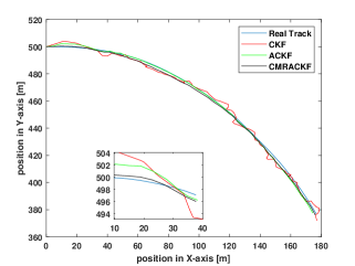
Figure 1: Target tracking result for position and its estimation.

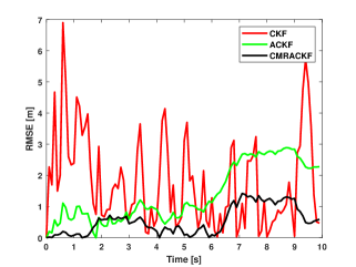
Figure 2: Position RMSE of considered algorithms.

Figure 1 depicts the tracking accuracy with CKF, ACKF, proposed algorithm, it can be observed that CKF can not track the true state ($x_{1,k}$). Nevertheless, the ACKF (green) and proposed algorithm (black) can track position $x_{1,k}$ accurately shown in zoomed version too.

Figure 2 shows the position RMSE error of CKF, ACKF and proposed method for target tracking. It can be observed that the CKF is having larger estimation error owing to fixed values of noise covariance, $Q$ and $R$. The average RMSE values of CKF, ACKF and the proposed algorithms are calculated as $1.79m$, $1.40m$ and $0.55m$, respectively. However, CMRACKF algorithm outperforms the CKF and ACKF. In conclusion, the CMRACKF algorithm has better tracking ability.

6 Conclusions

The summary of the paper presents a novel CMRACKF algorithm. In the proposed algorithm, moving window method based on covariance matching is applied to evaluate the the measurement noise co-variance matrix that can adaptively adjust statistical noise parameters on-line. The noise covariance matrices is used, then feedback to the standard ACKF to overcome the limitation of ACKF. Numerical simulation results reveal that the covariance matching framework RACKF can reduce the RMSE by 10% approximately and it can enhance the adaptive capability of ACKF algorithm.

References

• [1] M.ย S. Grewal and A.ย P. Andrews, Kalman filtering: Theory and Practice with MATLAB. John Wiley & Sons, 2014.
• [2] M.ย Cui, H.ย Liu, and W.ย Liu, โ€œAn adaptive unscented Kalman filter-based adaptive tracking control for wheeled mobile robots with control constrains in the presence of wheel slipping,โ€ International Journal of Advanced Robotic Systems, vol.ย 13, no.ย 5, pp.ย 1โ€“15, 2016.
• [3] E.ย A. Wan and R.ย Van Derย Merwe, โ€œThe unscented Kalman filter for nonlinear estimation,โ€ in Adaptive Systems for Signal Processing, Communications, and Control Symposium, pp.ย 153โ€“158, IEEE, 2000.
• [4] I.ย Arasaratnam and S.ย Haykin, โ€œCubature Kalman filters,โ€ IEEE Transactions on automatic control, vol.ย 54, no.ย 6, pp.ย 1254โ€“1269, 2009.
• [5] Y.ย Meng, S.ย Gao, Y.ย Zhong, G.ย Hu, and A.ย Subic, โ€œCovariance matching based adaptive unscented Kalman filter for direct filtering in INS/GNSS integration,โ€ Acta Astronautica, vol.ย 120, pp.ย 171โ€“181, 2016.
• [6] S.ย Gao, W.ย Wei, Y.ย Zhong, and A.ย Subic, โ€œSage windowing and random weighting adaptive filtering method for kinematic model error,โ€ IEEE Transactions on Aerospace and Electronic Systems, vol.ย 51, no.ย 2, pp.ย 1488โ€“1500, 2015.
• [7] A.ย Mohamed and K.ย Schwarz, โ€œAdaptive Kalman filtering for INS/GPS,โ€ Journal of geodesy, vol.ย 73, no.ย 4, pp.ย 193โ€“203, 1999.
• [8] B.ย Xia, H.ย Wang, Y.ย Tian, M.ย Wang, W.ย Sun, and Z.ย Xu, โ€œState of charge estimation of lithium-ion batteries using an adaptive cubature Kalman filter,โ€ Energies, vol.ย 8, no.ย 6, pp.ย 5916โ€“5936, 2015.
• [9] Q.ย Zhenbing, Q.ย Huaming, and W.ย Guoqing, โ€œAdaptive robust cubature kalman filtering for satellite attitude estimation,โ€ Chinese Journal of Aeronautics, vol.ย 31, no.ย 4, pp.ย 806โ€“819, 2018.
• [10] M.ย Narasimhappa, S.ย L. Sabat, and J.ย Nayak, โ€œFiber-optic gyroscope signal denoising using an adaptive robust Kalman filter,โ€ IEEE Sensors Journal, vol.ย 16, no.ย 10, pp.ย 3711โ€“3718, 2016.