Dynamic group testing to control and monitor disease progression in a population

Abstract

In the context of a pandemic like COVID-19, and until most people are vaccinated, proactive testing and interventions have been proved to be the only means to contain the disease spread. Recent academic work has offered significant evidence in this regard, but a critical question is still open: Can we accurately identify all new infections that happen every day, without this being forbiddingly expensive, i.e., using only a fraction of the tests needed to test everyone everyday (complete testing)?

Group testing offers a powerful toolset for minimizing the number of tests, but it does not account for the time dynamics behind the infections. Moreover, it typically assumes that people are infected independently, while infections are governed by community spread. Epidemiology, on the other hand, does explore time dynamics and community correlations through the well-established continuous-time SIR stochastic network model, but the standard model does not incorporate discrete-time testing and interventions.

In this paper, we introduce a “discrete-time SIR stochastic block model” that also allows for group testing and interventions on a daily basis. Our model can be regarded as a discrete version of the continuous-time SIR stochastic network model over a specific type of weighted graph that captures the underlying community structure. We analyze that model w.r.t. the minimum number of group tests needed everyday to identify all infections with vanishing error probability. We find that one can leverage the knowledge of the community and the model to inform nonadaptive group testing algorithms that are order-optimal, and therefore achieve the same performance as complete testing using a much smaller number of tests.

I Introduction

COVID-19 has revealed the key role of accurate epidemiological models and testing in the fight against pandemics[1, 2, 3, 4, 5, 6]. For any new disease or variant of the existing ones, we will always need to fast develop strategies that allow efficient testing of populations and empower targeted interventions. This poses several daunting challenges: (i) we need to test populations not just once but in a continual manner (on a daily basis), and (ii) we need to estimate the epidemic state of each individual and isolate only the infected ones. And all these, under the accuracy and cost limitations imposed by the various types of tests.

Recent works have identified the significance of proactive testing and individual-level intervention for the control of the disease spread (e.g. [7, 8, 9]), but to the best of our knowledge none of them addresses the challenges above efficiently. Most solutions rely on the idea of "testing everyone individually", which is inefficient for two reasons: on one hand, using cheap rapid testing usually results in many people (false positives) ending up in isolation without reason and at non-negligible societal cost; on the other hand, using accurate tests like PCR can be forbiddingly expensive. As a result, these works need to either neglect the cost of the former or alleviate the cost of the latter by scheduling tests on a (bi)weekly or monthly basis.

Therefore, a critical question is still open: can we use accurate/expensive tests more efficiently? In other words, can we identify all new infections that happen each day (complete testing performance), using significantly fewer accurate/expensive tests than complete testing? Complete accurate testing (e.g. PCR) on a daily basis and isolation of infected individuals can significantly reduce the number of infected people, as the example in Fig. 1 illustrates. Note that even with complete testing new infections still occur due to the delay between testing and receiving the test results (Fig. 1 assumes the usual delay of one day). Still, this is the best performance we can hope for, both in terms of containing infection and alleviating the societal impact of "false" quarantines; we thus ask how many tests do we really need to replicate it.

Traditional group testing strategies offer a powerful toolset for minimizing the number of tests, but they do not account for the time dynamics of a disease spread and do not take into account community structure. When the number of available tests is limited, two strategies are usually applied: sample testing, which tests only a sample of selected individuals, and/or group testing, which pools together diagnostic samples to reduce the number of tests needed to identify infected individuals in a population (e.g., see [10] and references therein). Both examine a static scenario: the state of individuals is fixed (infected or not), and the goal is to identify all infected ones.

To the best of our knowledge, our work in [11] was the first paper that targeted community-aware, group-test design for the dynamic case. In that work we used the well-established continuous-time SIR stochastic network model in [12], where individuals are regarded as the vertices of a graph $\mathcal{G}$ and an edge denotes a contact between neighboring vertices, and explored group testing strategies that were able to track the epidemic state evolution at an individual level, using a small number of tests. However, due to the complexity of the continuous time model, we were not able to provide theoretical guarantees for the minimum number of tests, and although we did consider testing delays, we left interventions for future work.

In this paper, we allow interventions, we use discrete-time SIR models for disease spread and we derive theoretical guarantees. Discrete time models fit more naturally with testing and intervention (which happen at discrete time-intervals), and are more amenable to analysis enabling methods to derive guarantees on the number of tests needed to achieve close-to-complete-testing accuracy. In this paper we use a model called the “discrete-time SIR stochastic block model,” which can be considered as a discrete version of the continuous-time SIR stochastic network model over a specific type of weighted graph. The graph used captures knowledge of an underlying community structure, as discussed in Section III. In Appendix A, we compare the continuous-time model from [12] with the discrete-time model introduced in our work and justify the use of our discrete-time model. We also note that our results are applicable to a larger set of SIR models, as discussed in Section IV-C.

Our main conclusion is that we can leverage the knowledge of the community and the dynamic model to inform group testing algorithms that are order-optimal and use a much smaller number of tests than complete testing to achieve the same performance. We arrive at this conclusion building on the following contributions.

We first argue that for discrete-time SIR models, given test results that identify the infection state the previous day, the problem of identifying the new infections each day reduces to static-case group testing with independent (but not identical) priors. So, existing nonadaptive algorithms such as CCA and/or random testing [13] can be reused. Figure 2 illustrates the sequence of events taking place on each day $t$.

We then derive a new lower bound (Theorem 2) for the number of tests needed in the case of independent (but not identical) priors. The main benefit of the new bound is not on "improving" upon the well-known entropy lower bound (stated as Lemma 1), but having a form that allows to prove order-optimality of group testing algorithms. In particular, we can prove that under mild assumptions existing nonadaptive algorithms are order-optimal in the static case (Corollary 2). This, in our opinion, is an interesting result on its own, since non-identical priors static group testing remains a relatively unexplored field compared to i.i.d. probabilistic group testing.

Finally, we derive conditions on the discrete-time SIR stochastic block model parameters under which order-optimal group test designs for the static case are also optimal for the dynamic case (Theorem 3). Simulation results show that indeed under these conditions we can achieve the performance of complete individual testing using a much smaller (close to the entropy lower bound) number of tests; for example, over a period of $50$ days, group testing needs an average of around $100$ tests per day for a population of $1000$ individuals. Our simulations use existing non-adaptive test designs - we do not derive new code designs as the existing ones are sufficient. However, we do use marginal probabilities derived daily from the SIR model to inform the group design: that is, the group tests we use vary from day to day, and their design leverages the knowledge of the underlying system dynamics that depend on the community structure, as well as the previous day test results.

The rest of the paper is organized as follows: Section II discusses related work; Section III provides our setup and background; Sec IV contains our main results; Section V provides numerical evaluation and concludes the paper.

Figure 1: Discrete-time SIR stochastic block model simulated on a population of 1000 individuals. Notice that without any testing or intervention a large fraction of the population gets infected. With complete testing (individually testing everyone everyday) and intervention (isolating individuals who are identified as infected) we can flatten the curve to a large extent. We assume that test results are only available the next day; if the test results were instantaneous we can identify all infections on the first day and isolate them and there would be no subsequent new infections.

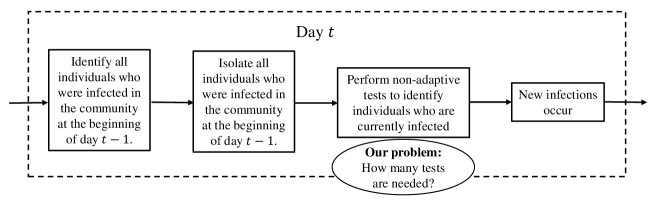
Figure 2: The dynamic testing problem with daily interventions. How many tests are needed to achieve complete testing performance everyday, given that test results become available after a day’s delay.

II Related Work

As stated in our introduction, our work shares similar goals with our prior work in [11], where we considered the well established continuous-time SIR stochastic network model (see [12]) and focused on how many tests to use and whom to test in order to track the infected individuals in the population. That work also explored how well one can learn the infected individuals given delayed test results, but gave no theoretical guarantees on the methods and did not consider intervention. Our discrete-time model for disease spread in this work, however, is more amenable to analysis and illustrates better the usefulness of group testing, being at the same time useful for practical reasons (more about this in Section III). We further note that our results are applicable to a more general set of SIR models as discussed in Section IV-C, remark 2.

Our model is closely related to the independent cascade model (see for example [14] and references therein), studied in the context of influence maximization in social networks, where we can interpret influence/rumor propagation as infections in our context. A crucial difference of our model from this is that our model allows multiple opportunities of infections over time whereas the independent cascade model only allows one opportunity to "infect". Therefore, as is noted, in our model the infectious individuals remain infectious until recovered or isolated.

The work in [15] considers a discrete stochastic model for the progression of COVID-19 based on contact networks and leverages the model dynamics to inform a group test decoder; however their scope is different, as they test infrequently and thus infections are highly correlated, do not consider interventions, do not look for optimal group test designs, and do not provide theoretical guarantees on the number of tests needed.

Since we use the main principles of the SIR model our work is closely related to epidemic modeling. Works in epidemiology discuss the implications of testing and intervention for COVID-19 employing stochastic network models (see [9, 8] and references therein) but do not consider test designs that exploit the knowledge of the underlying dynamical system. Works in control theory (see [16] and references therein) consider deterministic SIR compartment models (at the population level) and focus on intervention schemes. Here we are interested in both testing and intervention and use an individual-level SIR model.

Our work can be positioned in the general context of community-aware group testing where infected are not independent, and correlations follow from the community structure. Our work in [17, 18] demonstrated that using a known community structure to design group testing strategies and decoding, can significantly extend the advantages of group testing by utilizing these structural dependencies. Concurrently, the works in [19, 15] proposed decoding algorithms that take the community structure into account. Following up on these works in the static case (without temporal dynamics), there have been other recent works with similar goals [20, 21, 22]. Our work also leverages a known community structure that informs the system dynamics as well as the group test designs.

Further related to static group testing is the work on graph-constrained group testing (see for example [23], [24]), which solves the problem of how to design group tests when there are constraints on which samples can be pooled together, provided in the form of a graph. In our case, no such constraints exist and individuals can be pooled together into tests freely.

III Preliminaries and problem formulation

In this section we formalize our setup. Since our work for the dynamic case builds upon existing ones from static group testing, we first review some major results in that area that we also reuse in our paper (Section III-A). We then provide our model (Section III-C) and problem formulation (Section III-C).

III-A Preliminary: review of results from static group testing

Traditional group testing typically assumes a population of $N$ individuals out of which some are infected. Three infection models are typically considered: (i) in the combinatorial priors model, a fixed number of infected individuals $\mathit{k}$, are selected uniformly at random among all sets of size $\mathit{k}$; (ii) in i.i.d probabilistic priors model, each individual is i.i.d infected with probability $p$; (iii) in the non-identical probabilistic priors model, each item $i$ is infected independently of all others with prior probability $p_{i}$, so that the expected number of infected members is $\bar{\mathit{k}}=\sum_{i=1}^{N}p_{i}$ [13]. In this paper we mostly use results that apply to the last case.

A group test $\mathit{\tau}$ takes as input samples from $n_{\mathit{\tau}}$ individuals, pools them together and outputs a single value: positive if any one of the samples is infected, and negative if none is infected. More precisely, let ${U_{i}=1}$ when individual $i$ is infected and $0$ otherwise. Then the group testing output $\mathit{y}_{\mathit{\tau}}$ takes a binary value calculated as $\mathit{y}_{\mathit{\tau}}=\bigvee_{i\in\mathcal{D}_{\mathit{\tau}}}\mathit{U}_{i}$, where $\bigvee$ stands for the OR operator (disjunction) and $\mathcal{D}_{\mathit{\tau}}$ is the group of people participating in the test.

The usual goal in static group testing is to design a testing algorithm that is able to identify all infection statuses $\mathbf{U}=\left(U_{1},\ldots,U_{N}\right)$. These algorithms can be adaptive or non-adaptive. Adaptive testing uses the outcome of previous tests to decide what tests to perform next. An example of adaptive testing is binary splitting, which implements a form of binary search. Non-adaptive testing constructs, in advance, a test matrix $G\in\{0,1\}^{\mathit{T}\times N}$ where each row corresponds to one test, each column to one member, and the non-zero elements determine the set $\mathcal{D}_{\mathit{\tau}}$. Although adaptive testing uses less tests than non-adaptive, non-adaptive testing is often more practical as all tests can be executed in parallel.

The main challenge in static group testing is the number of group tests $\mathit{T}=\mathit{T}(N)$ needed to identify the infected members without error or with high probability. In the following, we present some well established results that we reuse in our work (hereafter we use typical asymptotic notations; i.e., $f(n)=O(g(n)$, $f(n)=\Omega(g(n))$, or $f(n)=\Theta(g(n))$ respectively means that a $f(n)\leq cg(n)$, $f(n)\geq cg(n)$, $c_{1}g(n)\leq f(n)\leq c_{2}g(n)$ asymptotically, where $c$, $c_{1}$, $c_{2}$ are universal constants):

$\bullet$ For the probabilistic model (ii), any non-adaptive algorithm with a success probability bounded away from zero as $N\rightarrow\infty$ must have $\mathit{T}=\Omega\left(\min\{\bar{\mathit{k}}\log{N},N\}\right)$ [25, Theorem 1],[26]. This means that either any non-adaptive group testing with a number of tests $O(\bar{\mathit{k}}\log{N})$ is order optimal, or individual testing is order optimal. In particular, random test designs, such as i.i.d. Bernoulli [28, 29, 30] and near-constant tests-per-item [31, 32] have been proved to be order-optimal in a sparse regime where $\bar{\mathit{k}}=\Theta(N^{\alpha})$ and $\alpha\in(0,1)$. In fact, in the same regime, [26] has provided the precise constants for optimal non-adaptive group testing. Conversely, classic individual testing has been proved to be optimal in the linear ($\bar{\mathit{k}}=\Theta(N)$) [33] and the mildy sublinear regime ($\bar{\mathit{k}}=\omega(\frac{N}{\log N})$) [25].

$\bullet$ For the probabilistic model (iii), a lower bound for the number of tests needed is given by the entropy, stated below:

Lemma 1 (Entropy lower bound).

Consider the non-identical probabilistic priors model of static group testing, where each individual $i\in[N]$ is infected independently with probability $p_{i}$. The number of tests $T$ needed by a non-adaptive algorithm to identify the infection status of all individuals with a vanishing probability of error satisfies

$$T\geq\sum_{i=1}^{N}\mathit{h_{2}}\left(p_{i}\right),$$

where $\mathit{h_{2}}(\cdot)$ is the binary entropy function.

See Appendix A in [13] for a proof. On the algorithmic side, two known algorithms are: the adaptive laminar algorithms that need at most $2\sum_{i=1}^{N}\mathit{h_{2}}\left(p_{i}\right)+2\bar{\mathit{k}}$ tests on average, and the “Coupon collector” nonadaptive algorithm (CCA) that needs at most $\mathit{T}\leq 4e(1+\delta)\bar{\mathit{k}}\ln{N}$ test to achieve an error probability no larger than $2N^{-\delta}$ whenever $p_{i}\leq\nicefrac{{1}}{{2}}$  [13, 34].

Distinction from traditional group testing. In this paper, we focus on probabilistic infections and non-adaptive test designs, but we differ from traditional group testing in two ways:
(a) Traditional group testing examines a static scenario, where the state of individuals is fixed (infected or not); we are instead interested in a dynamic scenario, where the state of an individual may change, even during the test period. This is particularly true since test results may not be available instantaneously but instead with a delay (e.g. after one day).
(b) The infection probabilities $p_{i}$ are not independent; instead, they are correlated where the correlation is induced by the underlying community structure and dynamic infection spread model we consider (for instance, two individuals who live in the same household are more likely to be both infected or not). This implies that $U_{i}$ and $U_{j}$ are not independent, as is the assumption in traditional group testing.

III-B Discrete-time SIR stochastic block model

We now describe our infection model via the discrete-time SIR stochastic block model with parameters $(N,C,q_{1},q_{2},p_{\mathrm{init}})$. Consider a population of size $N$ that is partitioned into multiple communities of size $\mathit{C}$. For simplicity we assume that $\nicefrac{{N}}{{\mathit{C}}}$ is an integer. On any day $t\in\mathbb{N}$, each individual can be in one of three states: Susceptible ($\mathcal{S}$), Infected ($\mathcal{I}$) or Recovered ($\mathcal{R}$). Let $\mathit{X}_{i}^{(t)}\in\{\mathcal{S},\mathcal{I},\mathcal{R}\}$ denote the state of individual $i$ on day $t$, and define the state of the system as ${\mathbf{X}}^{(t)}\triangleq(\mathit{X}_{1}^{(t)},\mathit{X}_{2}^{(t)},...,\mathit{X}_{N}^{(t)}).$ A small number of individuals are initially infected, and all new infections occur during “transmissible contacts” between infected and susceptible individuals. Recoveries occur independent of infections.

More precisely, on day $t=0$, every individual is i.i.d infected with probability $p_{\mathrm{init}}$. The following steps repeat everyday starting at $t=1$:

• An infected individual in some community infects a susceptible one from the same community w.p. $\mathit{q}_{1}$, independently of the other infected individuals of the community.

• An infected individual in some community infects a susceptible one from another community w.p. $\mathit{q}_{2}$, independently from all other infected individuals.

• An infected individual recovers independently from all other individuals w.p. $\mathit{r}$.

The discrete-time SIR stochastic block model can be envisioned as a discrete version of the well-established continuous-time SIR stochastic network model [12] on the corresponding weighted graph. It inherits the main properties from the latter; for example, infections are transmitted only from an infected to a susceptible individual and both infections and recoveries are stochastic. The main difference is that in the continuous-time one, the infections and the recoveries happen according to continuous-time Markovian process with transmissibility rate $\mathit{\beta}$ and recovery rate $\mathit{\gamma}$, which means that the time until a new state transition ($\mathcal{S}\rightarrow\mathcal{I}$ or $\mathcal{I}\rightarrow\mathcal{R}$) is exponentially distributed (with mean $\mathit{\beta}$ or $\mathit{\gamma}$ respectively). Indeed this makes the event that an individual got infected and subsequently recovered within a single day possible in the continuous-time model, whereas this is impossible in our discrete-time model.

Learning the intra-community and inter-community structure to model infection transmissions is, we believe, also practically feasible. Close contact “community” data is often readily available; for example students in each classroom in a school could form a community, and so could workers in the same office space. We also note that community-level network models alleviate some of the privacy concerns associated with using contact tracing data which tracks the exact pairs of individuals who come in contact with each other on a daily basis.

A useful remark about our model is that the state of an individual $\mathit{X}_{i}^{(t)}\in\{\mathcal{S},\mathcal{I},\mathcal{R}\}$ is different from the infection state $\mathit{U}_{i}^{(t)}\in\{0,1\}$, where $1$ (resp. $0$) corresponds to the “infected” (resp. “not infected”). Indeed $U_{i}^{(t)}=1$ iff $\mathit{X}_{i}^{(t)}=\mathcal{\mathcal{I}}$. This difference is important in our context, because our tests do not distinguish between susceptible and recovered individuals. In the remainder of the paper, $\mathit{X}_{i}^{(t)}$ will be called the “SIR state” of individual $i$, while $U_{i}^{(t)}$ will be $i$’s “infection status.” As a result, whether a individual is infected or not changes with the day, and thus we now consider a random variable $U_{i}^{(t)}$ associated with each individual that describes whether it is infected on day $t$ ($t\in\mathbb{\mathbb{missing}}{N}$).

III-C The dynamic testing problem formulation

As can be seen from Fig. 1, testing everyone, everyday, and isolating infected individuals helps drastically reduce the number of infections that happen on a given day. We assume that the results of a test administered on a particular day are available only the next day (as usually is the case with classic PCR testing for SARS-COV-2). We also isolate only the individuals who test positive, and we do so as soon as the test results are available. Moreover, we bring back the isolated individual into the population only when they are completely recovered. Note that in the SIR model, recovered individuals cannot get infected and play no role in transmitting the infection. Therefore, without loss of generality, we could assume that isolated individuals remain isolated for the rest of the testing period.

Given these assumptions, the question we ask is if complete testing is necessary to identify all new infections everyday, or if we can achieve the same performance as complete testing with significantly fewer number of tests. In particular, how many non-adaptive group tests are necessary and sufficient to identify all new infections (with a vanishing error probability) on each day? Our problem formulation is depicted in Fig. 2.

To aid a precise mathematical formulation for the problem, we first introduce some notation.

• $I^{(t)}_{j}$: number of new infections in community $j$ that occurred on day $t$. Note that in the set-up of Fig. 2, this number is also equal to the number of infected individuals remaining in community $j$ after intervention has been decided for day $t+1$. The new infections which happened on day $t$ will only be identified by the tests administered on day $t+1$, whose results are available only on day $t+2$.

• $p_{j}^{(t)}$: the probability of an individual in community $j$ who was susceptible at the end of day $t-1$ getting infected on day $t$. Note that this is same for every such individual in community $j$, by symmetry of the model. Moreover, we can calculate this probability as

  $$p_{j}^{(t)} =1-\mbox{${\mathbb{P}}$}(\text{individual is not infected on day }t)$$

  $$=1-(1-q_{1})^{I_{j}^{(t-1)}}(1-q_{2})^{\sum_{j^{\prime}\neq j}I^{(t-1)}_{j^{\prime}}}.$$

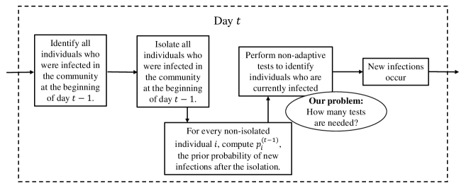
Figure 3: From dynamic to static testing: on day $t$ we perfectly learn the states of all non-isolated individuals at the time of testing on the previous day $t-1$. Given this information, we know that each susceptible individual in community $j$ is later infected with probability $p_{j}^{(t-1)}$ independent of every other individual. How many tests are needed to attain a vanishing probability of error on this non-identical static group testing problem?

Reduction to static group testing with non-identical probabilistic priors. Note that given $I_{j}^{(t-1)}\ \forall j$, an individual belonging to community $j$ is infected independently of every other individual with probability $p_{j}^{(t)}$ on day $t$. Thus, conditioned on the infection status of all individuals on day $t-1$, the infections which happen on day $t$ are independent (but not identically distributed). Now in our dynamic testing problem set-up, on day $t$ we perfectly learn the infection statuses of all non-isolated individuals at the time of testing on the previous day $t-1$. Given this information, we can exactly calculate the $p_{j}^{(t-1)}\ \forall j$ (see Fig. 3), i.e. the probability that each susceptible individual in community $j$ was later infected because of the non-isolated infected individuals.

So, given accurate test results, the dynamic testing problem is transformed daily to the problem of static group testing with non identical probabilistic priors (model (iii) in Section III-A). Therefore, the precise question we are after is the following: given that each individual in community $j$ is infected with probability $p_{j}^{(t)}$ independently of every other individual, how many tests are necessary and sufficient to learn the infection status with a vanishing probability of error? We answer this question in the next section.

IV Main results

In this section, we prove our main theoretical results. For brevity, we will use the terms “i.i.d. priors” and “non-identical priors” to refer to i.i.d probabilistic priors model (ii) and non identical probabilistic priors model (iii) from Section III-A, respectively. The contents of this section are ordered as follows:

• First, we provide a new lower bound on the number of tests required for the problem of static group testing with non i.i.d probabilistic priors (Theorem 2). To prove Theorem 2, we use two intermediate results: (a) we show that any test design that “works” for a given prior probabilities of infection $(p_{1},p_{2},...,p_{N})$ also works for the reduced prior probabilities $(p_{1}^{\prime},p_{2}^{\prime},...,p_{N}^{\prime})$ where $p_{i}^{\prime}\leq p_{i}\leq 0.5\ \forall i$. In words, we essentially prove that group testing is easier when the infections are sparser (Theorem 1); and (b) we show the following interesting property of the optimal decoder (Lemma 3) – if the optimal decoder correctly infers all the infection statuses when a set $\mathcal{D}$ is the set of infected individuals, then it will also correctly infer all the infection statuses when $\mathcal{D}^{\prime}\subset\mathcal{D}$ is the set of infected individuals.

• Second, we use simple asymptotic arguments to show that some existing group testing strategies (such as CCA [13] for non-identical priors and random testing for i.i.d priors) are order-optimal for non-identical priors (Corollary 2), when $p_{\max}=O(p_{\min})$, where $p_{\max}$ is the maximum entry in $(p_{1},p_{2},...,p_{N})$ and $p_{\min}$ is the minimum entry. The order $O(\cdot)$ is order with respect to the size of the population $N$.

• Finally, in Theorem 3, we bridge the gap between our dynamic testing problem formulation and the above static testing problem by showing that if $q_{1}=O(q_{2})$, $p_{\mathrm{init}}\leq 0.5$ and if $q_{1}\leq\frac{1-1/\sqrt{2}}{\mathit{C}}$ and $q_{2}\leq\frac{1-1/\sqrt{2}}{N}$, then the above two conditions on the prior vector are satisfied everyday in the discrete-time SIR stochastic block model parameterized by $(N,C,p_{\mathrm{init}},q_{1},q_{2})$. As a result the existing group testing strategies discussed above are order-optimal even for the dynamic testing problem formulation considered, provided that we use a sufficient number of tests each day to identify all new infections for that day.

IV-A Results on static group testing with non i.i.d priors

We first consider the problem of static group testing, in which a person is infected independently with a known prior probability $p_{i}$. Denote by $\mathbf{p}=(p_{1},p_{2},...,p_{N})$ the prior vector which collects the prior probabilities of infection of all individuals. We first define some notation specific to this subsection:

• $G$: test matrix

• $\mathcal{D}$: set of defectives or infections

• $\mathbf{U}=(U_{1},U_{2},...,U_{N})$: infection status configuration, i.e., individual $i$ is infected if and only if $U_{i}=1$.

• $\mathbf{U}(\mathcal{D})\triangleq(U_{1},...,U_{N})$ where $U_{i}=1$ iff $i\in\mathcal{D}$. Basically represents the vector notation for the set of infections given by $\mathcal{D}$. Note that there is a one-one correspondence between $\mathcal{D}$ and $\mathbf{U}(\mathcal{D})$. We will use these two notations interchangeably based on convenience.

• $G(\mathbf{U})$ represents the test results corresponding to the given test design and infection status configuration.

• For a fixed number of tests $T$, define a decoding function $R:\{0,1\}^{[T]}\rightarrow\{0,1\}^{[N]}$ which estimates the infection statuses from the test results.

• A defective set $\mathcal{D}$ “explains” test results $\mathbf{y}$ iff $G(\mathbf{U}(\mathcal{D}))=\mathbf{y}$.

• $\mbox{${\mathbb{P}}$}(\mathbf{U};\mathbf{p})$ denotes the probability of the infection status configuration under priors $\mathbf{p}$, i.e.

  $$\mbox{${\mathbb{P}}$}(\mathbf{U};\mathbf{p})=\prod_{i=1}^{N}p_{i}^{U_{i}}(1-p_{i})^{1-U_{i}}.$$

• Probability of error for a test matrix, decoder pair under given priors

  $$\mathbb{P}_{err}(G,R;\mathbf{p}) \triangleq\operatorname*{\mathbb{E}}_{\mathbf{U}\sim\mathbf{p}}\mathbbm{1}\{R(G(\mathbf{U}))\neq\mathbf{U}\}$$

  $$=\sum_{\mathbf{u}\in\{0,1\}^{N}}\mbox{${\mathbb{P}}$}(\mathbf{U}=\mathbf{u};\mathbf{p})\mathbbm{1}\{R(G(\mathbf{u}))\neq\mathbf{u}\}.$$

Definition 1 (MAP decoder).

For fixed priors $\mathbf{p}$ and testing matrix $G$ with number of tests $T$, we define the corresponding MAP decoder as $R_{map}(\ \cdot\ ;G,\mathbf{p}):\{0,1\}^{T}\rightarrow\{0,1\}^{N}$, where

$$R_{map}(\mathbf{y};G,\mathbf{p})=\operatorname*{arg\,max}\limits_{\mathbf{U}:G(\mathbf{U})=\mathbf{y}}\mbox{${\mathbb{P}}$}(\mathbf{U};\mathbf{p}).$$

In case of ties, the MAP decoder will select the solution which comes the earliest lexicographically.

In words, the MAP decoder chooses the most likely configuration which explains the test results. We next show that the MAP decoder is the optimal decoder for a fixed $G$ and $\mathbf{p}$, i.e., the MAP decoder minimizes the probability of error amongst all decoders for any $G$, $\mathbf{p}$.

Remark. Though the MAP decoder is optimal, it is unclear if the optimization problem corresponding to the MAP decoder can be solved efficiently. However, many heuristics such as belief propagation (see for example [17]) and random sampling methods exist which approximate well the MAP decoder. That said, in this work we use the MAP decoder only as a tool for theoretical analysis of the error probability.

Lemma 2 (Optimality of MAP decoder).

For given test matrix $G$ and priors $\mathbf{p}$, the corresponding MAP decoder minimizes the probability of error for the test matrix under the given priors, i.e.,

$$\mathbb{P}_{err}(G,R_{map}(\ \cdot\ ;G,\mathbf{p});\mathbf{p})\leq\mathbb{P}_{err}(G,R;\mathbf{p})\ \forall R.$$

We give the proof of Lemma 2 to Appendix B.

Given the optimality of the MAP decoder, we will denote by $\mathbb{P}_{err}^{*}(G,\mathbf{p})\triangleq\mathbb{P}_{err}(G,R_{map}(\ \cdot\ ;G,\mathbf{p});\mathbf{p}),$ the optimal probability of error corresponding to a given test design and priors.

We next prove a property of the MAP decoder, and this property will be used in the proof of our main result that follows. The following Lemma says that it is easier for the MAP decoder to identify a sparser defective set.

Lemma 3.

Consider a test matrix $G$ and priors $\mathbf{p}$. Suppose the corresponding MAP decoder is erroneous when identifying the defective set $\mathcal{D}$. Then the MAP decoder is also erroneous for the set of defectives is $\mathcal{D}\cup\{j\}$ with $p_{j}\leq 0.5$, i.e.,

$$\mathbbm{1} \left\{R_{map}\left(G(\mathbf{U}(\mathcal{D}\cup\{j\}));G,\mathbf{p}\right)\neq\mathbf{U}(\mathcal{D}\cup\{j\})\right\}$$

$$\geq\mathbbm{1}\left\{R_{map}(G(\mathbf{U}(\mathcal{D}));G,\mathbf{p})\neq\mathbf{U}(\mathcal{D})\right\}.$$

For the proof of Lemma 3, we refer the reader to Appendix C.

We next prove the main new result for the static case. In words, the following theorem says that the group testing problem is only easier when the infections are sparser. As a result, this allows us to lower/upper bound the group testing problem with non-identical priors by a group testing problem with identical priors.

Theorem 1.

Consider a testing matrix $G$ used with two different sets of priors $\mathbf{p}$ and $\mathbf{p}^{\prime}$. Further let $p^{\prime}_{i}=p_{i}$ for every $i\in[N],i\neq j$ and $p^{\prime}_{j}\leq p_{j}\leq 0.5$. The two prior vectors are same everywhere except at index $j$ where $\mathbf{p}^{\prime}$ is smaller. Then

$$\mathbb{P}_{err}^{*}(G,\mathbf{p}^{\prime})\leq\mathbb{P}_{err}^{*}(G,\mathbf{p}).$$

Proof.

We prove this by showing that when the MAP decoder corresponding to $(G,\mathbf{p})$ pair is used as a decoder with $(G,\mathbf{p}^{\prime})$, the probability of error is always lower, i.e.,

$$\mathbb{P}_{err}(G, R_{map}(\ \cdot\ ;G,\mathbf{p});\mathbf{p}^{\prime})$$

$$\leq\mathbb{P}_{err}(G,R_{map}(\ \cdot\ ;G,\mathbf{p});\mathbf{p})=\mathbb{P}_{err}^{*}(G,\mathbf{p}).$$

As a result the optimal decoder for $(G,\mathbf{p}^{\prime})$ pair has a probability of error not exceeding this quantity.

Now, we can express the probability of error for the MAP decoder of $(G,\mathbf{p})$ pair. For simplicity of notation in the following derivations, $\mathcal{E}(\mathcal{D})\triangleq\mathbbm{1}\left\{R_{map}(G(\mathbf{U}(\mathcal{D}));G,\mathbf{p})\neq\mathbf{U}(\mathcal{D})\right\}$ denotes the indicator of the event that the MAP decoder is erroneous when the defective set is $\mathcal{D}$ (and under further assumptions that the priors are $\mathbf{p}$ and test matrix is $G$).

$$\mathbb{P}_{err}(G,R_{map}(\ \cdot\ ;G,\mathbf{p});\mathbf{p})$$

$$=\sum_{\mathcal{D}\in[N]}\mbox{${\mathbb{P}}$}(\mathbf{U}(\mathcal{D}))\mathcal{E}(\mathcal{D})$$

$$=\sum_{\mathcal{D}\in[N]}\prod_{i\in\mathcal{D}}p_{i}\prod_{l\in[N]\setminus\mathcal{D}}(1-p_{l})\mathcal{E}(\mathcal{D})$$

$$\overset{(a)}{=}\sum_{\begin{subarray}{c}\mathcal{D}\in[N]\\ |j\in\mathcal{D}\end{subarray}}\prod_{i\in\mathcal{D}}p_{i}\prod_{l\in[N]\setminus\mathcal{D}}(1-p_{l})\mathcal{E}(\mathcal{D})$$

$$\hskip 8.5359pt+\sum_{\begin{subarray}{c}\mathcal{D}\in[N]\\ |j\notin\mathcal{D}\end{subarray}}\prod_{i\in\mathcal{D}}p_{i}\prod_{l\in[N]\setminus\mathcal{D}}(1-p_{l})\mathcal{E}(\mathcal{D})$$

$$\overset{(b)}{=}p_{j}\sum_{\begin{subarray}{c}\mathcal{D}\in[N]\setminus\{j\}\end{subarray}}\prod_{i\in\mathcal{D}}p_{i}\prod_{l\in[N]\setminus\mathcal{D}\cup\{j\}}(1-p_{l})\mathcal{E}(\mathcal{D}\cup\{j\})$$

$$\hskip 8.5359pt+(1-p_{j})\sum_{\begin{subarray}{c}\mathcal{D}\in[N]\setminus\{j\}\end{subarray}}\prod_{i\in\mathcal{D}}p_{i}\prod_{l\in[N]\setminus\mathcal{D}\cup\{j\}}(1-p_{l})\mathcal{E}(\mathcal{D}),$$ (1)

where in $(a)$ we split the summation into two cases – one where $j\in\mathcal{D}$ and the other where $j\notin\mathcal{D}$; in $(b)$ we take $j$ out of the summation.

Similarly, one could express the probability of error for the same decoder with the pair $(G,\mathbf{p}^{\prime})$ as

$$\mathbb{P}_{err}(G,R_{map}(\ \cdot\ ;G,\mathbf{p});\mathbf{p}^{\prime})$$

$$=p^{\prime}_{j}\sum_{\begin{subarray}{c}\mathcal{D}\in[N]\setminus\{j\}\end{subarray}}\prod_{i\in\mathcal{D}}p_{i}\prod_{l\in[N]\setminus\mathcal{D}\cup\{j\}}(1-p_{l})\mathcal{E}(\mathcal{D}\cup\{j\})$$

$$\hskip 2.84544pt+(1-p^{\prime}_{j})\sum_{\begin{subarray}{c}\mathcal{D}\in[N]\setminus\{j\}\end{subarray}}\prod_{i\in\mathcal{D}}p_{i}\prod_{l\in[N]\setminus\mathcal{D}\cup\{j\}}(1-p_{l})\mathcal{E}(\mathcal{D}).$$ (2)

The first error term $\mathbb{P}_{err}(G,R_{map}(\ \cdot\ ;G,\mathbf{p});\mathbf{p})$ is of the form $p_{j}a+(1-p_{j})b$, and the second error term $\mathbb{P}_{err}(G,R_{map}(\ \cdot\ ;G,\mathbf{p});\mathbf{p}^{\prime})$ is of the form $p^{\prime}_{j}a+(1-p^{\prime}_{j})b$. From Lemma 3, we have $\mathcal{E}(\mathcal{D}\cup\{j\})\geq\mathcal{E}(\mathcal{D})$ and hence $a\geq b$. Since $a\geq b$ and $p_{j}^{\prime}\leq p_{j}$, one can verify that $p_{j}a+(1-p_{j})b\geq p^{\prime}_{j}a+(1-p^{\prime}_{j})b$, and thus

$$\mathbb{P}_{err}(G,R_{map}(\ \cdot\ ;G,\mathbf{p});\mathbf{p})\geq\mathbb{P}_{err}(G,R_{map}(\ \cdot\ ;G,\mathbf{p});\mathbf{p}^{\prime}),$$

concluding the proof. ∎

Now one could repeatedly apply Theorem 1 on the prior vector $\mathbf{p}$ to conclude that any test matrix $G$ should only do better on the reduced uniform prior vector $\mathbf{p}_{\min}=(p_{\min},p_{\min},...,p_{\min})$ where $p_{\min}\triangleq\min_{i\in[N]}p_{i}$. On the other hand, the test matrix $G$ should only do worse on the prior vector $\mathbf{p}_{\max}=(p_{\max},p_{\max},...,p_{\max})$ where $p_{\max}\triangleq\max_{i\in[N]}p_{i}$. This is stated below without a formal proof.

Corollary 1.

Consider a test matrix $G$ and a prior vector $\mathbf{p}$ such that $p_{i}\leq 0.5$ for all $i\in[T]$. Let $\mathbf{p}_{\min}=(p_{\min},p_{\min},...,p_{\min})$ where $p_{\min}\triangleq\min_{i\in[N]}p_{i}$ and let $\mathbf{p}_{\max}=(p_{\max},p_{\max},...,p_{\max})$ where $p_{\max}\triangleq\max_{i\in[N]}p_{i}$. Then

$$\mathbb{P}_{err}^{*}(G,\mathbf{p}_{\max})\geq\mathbb{P}_{err}^{*}(G,\mathbf{p})\geq\mathbb{P}_{err}^{*}(G,\mathbf{p}_{\min}).$$

As a consequence of the above corollary, the number of tests required to attain a fixed (small) probability of error $\epsilon$ with prior vector $\mathbf{p}_{\min}$ is not more than the number of tests required to attain probability of error $\epsilon$ with prior vector $\mathbf{p}$. This observation allows us to use the lower bound on the number of tests when the priors are identical. This is made precise in the following theorem.

Theorem 2.

Consider the non-adaptive group testing problem with $N$ items where the probability of item $i$ being infected is $p_{i}\leq 0.5$. Let $p_{\min}\triangleq\min\limits_{i\in[N]}p_{i}$. In order to achieve a probability of error $\rightarrow 0$ as $N\rightarrow\infty$, the number of tests must be

$$T(\mathbf{p})=\Omega(\min\{N,Np_{\min}\log N\}).$$

Proof.

From Corollary 1, suppose a test matrix $G$ achieves a probability of error $\epsilon$ on prior vector $\mathbf{p}$, the same test matrix achieves a probability of error not more than $\epsilon$ on the prior vector $\mathbf{p}_{\min}$, where $\mathbf{p}_{\min}=(p_{\min},p_{\min},...,p_{\min})$ and $p_{\min}\triangleq\min_{i\in[N]}p_{i}$. Any strategy that achieves a probability of error $\rightarrow 0$ as $N\rightarrow\infty$ with the prior vector $\mathbf{p}_{\min}$ requires a number of tests equal to $\Omega(\min\{N,Np_{\min}\log N\})$. Thus, we need at least as many tests with the prior vector $\mathbf{p}$. ∎

As discussed in Section III-A, the entropy bound in Lemma 1 is an alternate lower bound on the number of tests needed for this problem. We note that the entropy bound might be greater or smaller than the term $Np_{\min}\log N$ in Theorem 2. In particular, if $p_{i}\leq 1/2\ \forall i$ it is easy to see that $\sum_{i=1}^{N}\mathit{h_{2}}(p_{i})\geq N\mathit{h_{2}}(p_{\min})\geq Np_{\min}\log\nicefrac{{1}}{{p_{\min}}}$. However the term $\nicefrac{{1}}{{p_{\min}}}$ may be smaller or larger than $N$; thus our bound, that applies independently of the value of $p_{\min}$ (as long as $p_{i}\leq 0.5$) cannot be directly derived from the entropy bound, and could be either greater or lesser than the entropy bound. Having said that, the main advantage of the lower bound in Theorem 2 is its particular form, which allows the proof of order-optimality of several static group testing algorithms, as we will see in the next subsection.

Now, if the prior vector $\mathbf{p}$ is “bounded”, in the sense that the maximum entry and minimum entry in $\mathbf{p}$ differ by a constant factor (constant with respect to $N$), then the lower bound can be re-written in terms of the maximum entry in $\mathbf{p}$ or the mean of $\mathbf{p}$. Basically we here just use the fact that constant factors do not affect the order. We next make this corollary precise.

Definition 2 (Bounded priors).

Let $\eta\in[1,\infty)$ be a fixed constant (constant with respect to $N$). A prior vector $\mathbf{p}$ of length $N$ is called $\eta-$bounded if

$$\frac{\max_{i}p_{i}}{\min_{i}p_{i}}\leq\eta.$$

Corollary 2 (Lower bound for bounded priors).

Consider the non-adaptive group testing problem with $N$ items where the probability of item $i$ being infected is $p_{i}\leq 0.5$. Let $p_{\max}\triangleq\max\limits_{i\in[N]}p_{i}$ and $p_{\operatorname*{mean}}\triangleq\frac{1}{N}\sum_{i=1}^{N}p_{i}$. Suppose $\mathbf{p}=(p_{1},...,p_{N})$ is $\eta$-bounded for some constant $\eta$. Any strategy that achieves a probability of error $\rightarrow 0$ as $N\rightarrow\infty$ requires

$$T(\mathbf{p}) =\Omega(\min\{N,Np_{\operatorname*{mean}}\log N\})$$

$$=\Omega(\min\{N,Np_{\max}\log N\}).$$

IV-B Performance of existing non-adaptive algorithms in the static non-identical priors

Suppose $\mathbf{p}$ is $\eta$-bounded and each $p_{i}\leq 0.5$. The following non-adaptive algorithms can be proved to be order-optimal with respect to the lower bound in Corollary 2:

• The Coupon Collector Algorithm (CCA) from [13] for prior vector $\mathbf{p}$, as discussed in Section III-A, achieves a probability of error less than $2N^{-\delta}$ with a number of tests less than $4e(1+\delta)Np_{\operatorname*{mean}}\log N$ (see Theorem 3 in [13]). As a result, w.r.t to the lower bound in Corollary 2, either CCA is order-optimal (if $N\geq Np_{\operatorname*{mean}}\log N$) or individual testing is order optimal (if $N\leq Np_{\operatorname*{mean}}\log N$).

• As discussed in Section III-A for the group testing problem with identical priors (say every item is infected with the same probability $p^{\prime}$), a variety of randomized and explicit algorithms have been proposed which achieve a vanishing probability of error with a number of tests $O(Np^{\prime}\log N)$. From Corollary 1, any test matrix that achieves a vanishing probability of error with $\mathbf{p}_{\max}$ should also attain a vanishing probability of error with $\mathbf{p}$, and as a result $O(Np_{\max}\log N)$ tests are sufficient for the prior vector $\mathbf{p}$. Consequently w.r.t our lower bound in Corollary 2, any of these designs is order optimal (if $N\geq Np_{\max}\log N$) or individual testing is order optimal (if $N\leq Np_{\max}\log N$).

IV-C Dynamic testing - bridging the gap

Given the discussion above, we next show conditions under which the prior probabilities of infections each day (these change everyday) are $\eta$-bounded and are each not more than $0.5$. If these two conditions are satisfied everyday for our discrete-time SIR stochastic block model set-up in Fig. 3, then CCA and the other algorithms discussed in Section IV-B are order-optimal for our dynamic testing problem formulation. (see 3). We first define some notation, building upon the notation in Section III-C.

• $p_{\max}^{(t)}\triangleq\max_{j}p_{j}^{(t)}$, the maximum probability of new infection on day $t$.

• $p_{\min}^{(t)}\triangleq\min_{j}p_{j}^{(t)}$, the minimum probability of new infection on day $t$.

Theorem 3.

Consider the testing-intervention problem in Fig. 3 where the infections follow the discrete-time SIR stochastic block model $(N,C,q_{1},q_{2},p_{\mathrm{init}})$.

• Suppose $p_{\mathrm{init}}\leq 0.5$, $q_{1}\leq\frac{1-1/\sqrt{2}}{\mathit{C}}$ and $q_{2}\leq\frac{1-1/\sqrt{2}}{N}$, then $p_{j}^{(t)}\leq 0.5$.

• Suppose $\frac{q_{1}}{q_{2}}\leq\eta$, then $\frac{p_{\max}^{(t)}}{p_{\min}^{(t)}}\leq\eta$ and as a result the prior vector for each day is $\eta$-bounded.

Proof.

We prove (i) first. We first have $p_{j}^{(0)}=p_{\mathrm{init}}\leq 0.5$. For $t\geq 1$, we have

$$p_{j}^{(t)} =1-(1-q_{1})^{I_{j}^{(t-1)}}(1-q_{2})^{\sum_{j^{\prime}\neq j}I^{(t-1)}_{j^{\prime}}}$$

$$\overset{(a)}{\leq}1-(1-q_{1})^{\mathit{C}}(1-q_{2})^{N}$$

$$\overset{(b)}{\leq}1-(1-\mathit{C}q_{1})(1-Nq_{2})\overset{(c)}{\leq}0.5,$$

where in $(a)$ we used the fact that the total number of infections inside a community and overall cannot be greater than $\mathit{C}$ and $N$, respectively; $(b)$ follows because of the algebraic inequality $(1+x)^{y}\geq 1+xy$ if $x\geq-1$ and $y\notin(0,1)$; in $(c)$ we used our assumptions about $q_{1}$ and $q_{2}$.

We next prove (ii). Since $q_{1}\geq q_{2}$ in our model, we have

$$p_{j}^{(t)} =1-(1-q_{1})^{I_{j}^{(t-1)}}(1-q_{2})^{\sum_{j^{\prime}\neq j}I^{(t-1)}_{j^{\prime}}}$$

$$=1-\left(\frac{1-q_{1}}{1-q_{2}}\right)^{I_{j}^{(t-1)}}(1-q_{2})^{\sum_{j^{\prime}}I^{(t-1)}_{j^{\prime}}}$$

$$\leq 1-\left(\frac{1-q_{1}}{1-q_{2}}\right)^{\max_{j}I^{(t-1)}_{j}}(1-q_{2})^{\sum_{j^{\prime}}I^{(t-1)}_{j^{\prime}}},$$ (3)

where $\max_{j}I^{(t)}_{j}$ is simply the maximum number of infections over all communities. Likewise,

$$p_{j}^{(t)} =1-(1-q_{1})^{I_{j}^{(t-1)}}(1-q_{2})^{\sum_{j^{\prime}\neq j}I^{(t-1)}_{j^{\prime}}}$$

$$\overset{(a)}{\geq}1-(1-q_{2})^{\sum_{j^{\prime}}I^{(t-1)}_{j^{\prime}}},$$ (4)

where in $(a)$ we used $q_{2}\leq q_{1}$. Combining (3) and (4) we have

$$\frac{p_{\max}^{(t)}}{p_{\min}^{(t)}} =\frac{1-\left(\frac{1-q_{1}}{1-q_{2}}\right)^{\max_{j}I^{(t-1)}_{j}}(1-q_{2})^{\sum_{j^{\prime}}I^{(t-1)}_{j^{\prime}}}}{1-(1-q_{2})^{\sum_{j^{\prime}}I^{(t-1)}_{j^{\prime}}}}$$

$$\overset{(a)}{\leq}\frac{1-\left(\frac{1-q_{1}}{1-q_{2}}\right)^{\max_{j}I^{(t-1)}_{j}}(1-q_{2})^{\max_{j}I^{(t-1)}_{j}}}{1-(1-q_{2})^{\max_{j}I^{(t-1)}_{j}}}$$

$$=\frac{1-(1-q_{1})^{\max_{j}I^{(t-1)}_{j}}}{1-(1-q_{2})^{\max_{j}I^{(t-1)}_{j}}}\overset{(b)}{\leq}\frac{q_{1}}{q_{2}}\leq\eta.$$

where $(a)$ follows from the following facts: the function $f_{1}(x)=\frac{1-\kappa x}{1-x}$ is increasing for $\kappa\in(0,1)$, the function $f_{2}(x)=(1-q_{2})^{x}$ is decreasing for $q_{2}\in(0,1)$, and the sum $\sum_{j^{\prime}}I^{(t-1)}_{j^{\prime}}$ is lower bounded by $\max_{j}I^{(t-1)}_{j}$; and $(b)$ follows from the fact that the function $f_{3}(x)=\frac{1-(1-q_{1})^{x}}{1-(1-q_{2})^{x}}$ is decreasing in $x\geq 1$ for $q_{1}\geq q_{2}$, and therefore the maximum of the ratio is obtained for $\max_{j}I^{(t-1)}_{j}=1$. All proofs of the above statements are provided in Appendix D. ∎

Finally, we make three remarks related to the results introduced in this section.
Remark 1. Both assumptions (i) and (ii) on the parameters in Theorem 3 will hold true when the number of communities is a constant, i.e., the size of each community is $C=\Theta(N)$ (as is the case when the population is well-mixed, or if we just consider a single community); assumption (i) does not require $C=\Theta(N)$. In our simulations, we observed empirically that assumption (ii) also holds when $C<<N$; we do not have a formal proof of Theorem 3 for this case however.
Remark 2. Our results hold not just for the specific model introduced in Section III (where in particular we assume symmetric intra and inter community transmissions) but for any underlying community structure where the two conditions (bounded prior vectors and the value of each prior not exceeding $\nicefrac{{1}}{{2}}$) are satisfied. For example, one could have a model where an infected individual can transmit the infection only to a subset of his fellow community members with probability $q_{1}$ (he/she cannot transmit to the rest of the individuals in his/her community) and only to a subset of individuals outside his/her community with probability $q_{2}$. For this example model, the conditions in Theorem 3 are sufficient to prove the two requirements on the prior vector.
Remark 3. Intervention is a crucial aspect for our results to hold true. Without intervention in our dynamic model, many of the prior probabilities would be greater than $\nicefrac{{1}}{{2}}$ and our requirements on the prior vector would not be satisfied.

V Numerical results

In this section, we show illustrative numerical results on the necessary and sufficient number of tests required for the discrete-time SIR stochastic block model. We next describe the experimental set-up.

• We simulate multiple instances (or trajectories) of the pipeline in Fig. 2 where the infections follow the discrete-time SIR stochastic block model $(N,C,p_{\mathrm{init}},q_{1},q_{2})$, and for different testing strategies. We simulate 200 trajectories and in Fig. 4, plot the daily average of the quantities across these trajectories.

• For each of these testing strategies, we empirically find the number of tests required on each day to identify all the infections on the previous day. To do this, on each day for a given trajectory, we start with 1000 tests and decrease this number (at a certain granularity) until the testing strategy makes a mistake. The smallest number of tests for which the strategy worked is plotted.

• On the other hand, we also plot the entropy lower bound in Lemma 1; it is easy to estimate this for our model via Monte-Carlo approximations. This bound holds for any set of values for $p_{i}^{(t-1)}$, regardless of whether the conditions required for Theorem 3 hold or not. The reason we use the entropy bound instead of our lower bound in Theorem 2 is that the entropy bound was numerically observed to be larger. Indeed, the lower bound in Theorem 2 contains some accompanying hidden constants which are small when used for our particular choice of $N$.

(a) $(N,C,p_{\mathrm{init}},q_{1},q_{2})=(1000,20,0.02,0.03,0.0004)$.

(b) $(N,C,p_{\mathrm{init}},q_{1},q_{2})=(1000,50,0.02,0.012,0.0004)$.

Figure 4: Experimental results. We plot the average number of tests required by each strategy to identify the infection statuses of all non-isolated individuals each day for 2 different sets of parameters.

We compare the following testing strategies in our numerical simulations.

• Complete testing. We test every non-isolated individual remaining in the population each day.

• Coupon Collector Algorithm (CCA) from [13]. We showed the order-optimality of this algorithm for the dynamic testing problem at the beginning of Section IV-C. In short, on each day, the CCA algorithm constructs a random non-adaptive test design which depends on $p_{j}^{(t)}$. The idea is to place objects which are less likely to be infected in more number of tests and vice-versa. We refer the reader to [13] for the exact description of the algorithm.

• Random group testing for max probability (Rnd. Grp. max.) Here we construct a randomized design assuming that each individual has a prior probability of infection $p_{\max}^{(t)}$. From Corollary 1, such a design must also work for the actual priors $p_{j}^{(t)}$. We construct a constant column-weight design (see e.g. [32]) where each individual is placed in $L=\lfloor\nicefrac{{T}}{{(Np_{\max}^{(t)}\log 2)}}\rfloor$ tests. Such a test design achieves a vanishing probability of error with $O(Np_{\max}^{(t)}\log N)$ tests (see for example [32] for a proof), and hence is order-optimal under the conditions in Theorem 3.

• Random group testing for mean probability (Rnd. Grp. mean) Here we construct a randomized design assuming that each individual has a prior probability of infection $p_{\operatorname*{mean}}^{(t)}$, where $p_{\operatorname*{mean}}^{(t)}$ is defined as the mean prior probability of infection across all individuals. Unlike Rnd. Grp. max., there is no guarantee on how many tests are needed by such a design to identify the infection statuses of all individuals. However, the numerical results in Fig. 4 show that such a design requires fewer tests than CCA or Rnd. Grp. max. designs.

The numerical results in Fig. 4 are illustrated for two different parameter values of the discrete-time SIR stochastic block model. In both cases, we see that Rnd. Grp. mean requires the least number of tests to identify the infection statuses of all non-isolated individuals. Moreover, the number of tests required by all three testing strategies considered is much less than the number required by complete testing. In fact the numerics in Fig. 4 indicate that if we use a number of tests equal to $\nicefrac{{1}}{{5}}$ of number of tests required for complete individual testing, all these algorithms would achieve the same performance as complete individual testing, at least for the particular examples that we considered.

A natural follow-up question to ask is if there is a systematic way to choose the number of tests that need to be administered, given the upper bounds discussed in Section IV-B. In Appendix E, we discuss one such heuristic and show that it achieves close-to-complete-testing performance.

VI Conclusions and open questions

In this work we proposed the problem of dynamic group testing which asks the question of how to continually test given that infections spread during the testing period. Our numerical results answer the question we started with – in the dynamic testing problem formulation, given a day of testing delay, is it possible to achieve close to complete testing performance with significantly fewer number of tests? The answer is yes, and in this paper we not only showed numerical evidence supporting this fact, but also gave theoretical bounds on the optimal number of tests needed in order to achieve this.

Although we gave theoretical bounds on the optimal number of tests needed each day, many open questions remain. In particular, it would be interesting to study the same problem when tests are noisy, or when we can use other models of group tests such as the one in [35], or simply when one cannot perfectly learn the states of all individuals on a testing day. In addition, it would also be of interest to study/use other test designs, for example like the ones in [27, 36, 28, 29, 30, 31, 32, 34, 37, 38, 39]. Finally, it remains open to see how these results translate to the continuous-time SIR stochastic network model of [12].

VII Acknowledgements

This work was supported in part by NSF grants #2007714, #1705077 and UC-NL grant LFR-18-548554. We also thank Katerina Argyraki for her ongoing support and the valuable discussions we have had about this project.

Appendix A Comparison of discrete and continuous-time SIR models

The well-studied continuous-time SIR stochastic network model from [12] has been the main motivation for our discrete-time SIR stochastic block model. In fact, the discrete-time SIR stochastic block model described in Section III-B can be considered as a discretized version of the continuous-time SIR stochastic network model over the weighted graph, where 2 individuals belonging to the same community are connected by an edge with weight $q_{1}$ and 2 individuals belonging to different communities are connected by an edge with weight $q_{2}$, and recoveries occur at the rate $r$/day – i.e., an infected individual transmits the disease to a susceptible individual in the same community at the rate $q_{1}$/day and to a susceptible individual in a different community at the rate $q_{2}$/day. In Fig. 5, we compare the continuous-time model above and the discrete-time model for a few example values of $q_{1}$, $q_{2}$ and $r$ for illustration.

Figure 5: Continuous vs discrete-time model. Continuous model in dashed and discrete model in solid curves. Recovery probability $r=0.1$ in all cases.

We make a few observations:
$\bullet$ The progression of the disease in the discrete-time and continuous-time models, though not identical, follow a similar pattern, justifying the use of the discrete-time model.
$\bullet$ In both the models, $\nicefrac{{1}}{{q_{1}}}$ is the expected time for an infected individual to transmit the disease to a susceptible individual in the same community, $\nicefrac{{1}}{{q_{2}}}$ is the expected time for an infected individual to transmit the disease to a susceptible individual in a different community and $\nicefrac{{1}}{{r}}$ is the expected time for an infected individual to recover.
$\bullet$ In the continuous-time model, an individual can get infected and recovered in the same day, whereas this is not possible in our discrete-time model (infected individuals can recover starting from the day after they are infected).

Appendix B Proof of Lemma 2

The optimality of the MAP decoder is a standard result in statistics and signal processing. We however give the proof in the context of our problem, for completeness.

See 2

Proof.

As stated at the beginning of Section IV, the Probability of error for a test matrix, decoder pair under given the priors is

$$\mathbb{P}_{err}(G,R;\mathbf{p}) \triangleq\operatorname*{\mathbb{E}}_{\mathbf{U}\sim\mathbf{p}}\mathbbm{1}\{R(G(\mathbf{U}))\neq\mathbf{U}\}$$

$$=\operatorname*{\mathbb{E}}_{\mathbf{Y}}\;\operatorname*{\mathbb{E}}_{\mathbf{U}|\mathbf{Y}}\mathbbm{1}\{R(G(\mathbf{U}))\neq\mathbf{U}\},$$

where $\mathbf{Y}$ is the set of test results. For the MAP decoder, the term inside $\operatorname*{\mathbb{E}}_{\mathbf{Y}}$ is

$$\operatorname*{\mathbb{E}}_{\mathbf{U}|\mathbf{Y}} \mathbbm{1}\{R_{map}(\mathbf{Y};G,\mathbf{p}))\neq\mathbf{U}\}$$

$$=\operatorname*{\mathbb{E}}_{\mathbf{U}|\mathbf{Y}}\mathbbm{1}\{\operatorname*{arg\,max}\limits_{\mathbf{U}:G(\mathbf{U})=\mathbf{Y}}\mbox{${\mathbb{P}}$}(\mathbf{U};\mathbf{p})\neq\mathbf{U}\}$$

$$=\sum_{\mathcal{D}\in\left[N\right]}\mbox{${\mathbb{P}}$}\left(\mathbf{U}(\mathcal{D})|\mathbf{Y};\mathbf{p}\right)$$

$$\hskip 34.14322pt\cdot\mathbbm{1}\{\operatorname*{arg\,max}\limits_{\mathbf{U}(\mathcal{D}):G(\mathbf{U}(\mathcal{D}))=\mathbf{Y}}\mbox{${\mathbb{P}}$}(\mathbf{U}(\mathcal{D});\mathbf{p})\neq\mathbf{U}(\mathcal{D})\}$$

$$=1-\mbox{${\mathbb{P}}$}\left(\operatorname*{arg\,max}\limits_{\mathbf{U}:G(\mathbf{U})=\mathbf{Y}}\mbox{${\mathbb{P}}$}(\mathbf{U}|\mathbf{Y};\mathbf{p})\right)$$

$$=1-\max_{\mathbf{U}:G(\mathbf{U})=\mathbf{Y}}\frac{\mbox{${\mathbb{P}}$}(\mathbf{U};\mathbf{p})}{\mbox{${\mathbb{P}}$}(\mathbf{Y})}.$$ (5)

Similarly, for any decoder $R$, we have

$$\operatorname*{\mathbb{E}}_{\mathbf{U}|\mathbf{Y}} \mathbbm{1}\{R(\mathbf{Y})\neq\mathbf{U}\}$$

$$=\sum_{\mathcal{D}\in\left[N\right]}\mbox{${\mathbb{P}}$}\left(\mathbf{U}(\mathcal{D})|\mathbf{Y};\mathbf{p}\right)\cdot\mathbbm{1}\{R(\mathbf{Y})\neq\mathbf{U}\}$$

$$=1-\mbox{${\mathbb{P}}$}\left(R(\mathbf{Y})|\mathbf{Y};\mathbf{p}\right)\geq 1-\max_{\mathbf{U}:G(\mathbf{U})=\mathbf{Y}}\frac{\mbox{${\mathbb{P}}$}(\mathbf{U};\mathbf{p})}{\mbox{${\mathbb{P}}$}(\mathbf{Y})}.$$ (6)

Comparing (5) and (6) concludes the proof. ∎

Appendix C Proof of Lemma 3

See 3

Proof.

We first state the trivial case where $\mathbbm{1}\left\{R_{map}(G(\mathbf{U}(\mathcal{D}));G,\mathbf{p})\neq\mathbf{U}(\mathcal{D})\right\}=0$. Under that assumption, the inequality of Lemma 3 always holds.

We then consider the case where $\mathbbm{1}\left\{R_{map}(G(\mathbf{U}(\mathcal{D}));G,\mathbf{p})\neq\mathbf{U}(\mathcal{D})\right\}=1$, i.e., the MAP decoder makes an error when the defective set is $\mathcal{D}$. In that case, one of the two situations is possible:

• there exists some set $\mathcal{D}^{\prime}\neq\mathcal{D}$, such that $G(\mathbf{U}(\mathcal{D}^{\prime}))=G(\mathbf{U}(\mathcal{D}))$ and $\mbox{${\mathbb{P}}$}(\mathbf{U}(\mathcal{D}^{\prime});\mathbf{p})>\mbox{${\mathbb{P}}$}(\mathbf{U}(\mathcal{D});\mathbf{p})$ or

• there exists some set $\mathcal{D}^{\prime}\neq\mathcal{D}$, such that $G(\mathbf{U}(\mathcal{D}^{\prime}))=G(\mathbf{U}(\mathcal{D}))$ and $\mbox{${\mathbb{P}}$}(\mathbf{U}(\mathcal{D}^{\prime});\mathbf{p})=\mbox{${\mathbb{P}}$}(\mathbf{U}(\mathcal{D});\mathbf{p})$ and $\mathcal{D}^{\prime}$ is lexicographically earlier than $\mathcal{D}$.

Hence MAP identifies incorrectly $\mathcal{D}^{\prime}$ as the defective set given that $\mathcal{D}$ was the true defective set. We prove assuming that the first situation occurred; the proof follows identical arguments for the second situation.

(a) $(N,C,p_{\mathrm{init}},q_{1},q_{2})=(1000,50,0.02,0.012,0.0004)$.

(b) $(N,C,p_{\mathrm{init}},q_{1},q_{2})=(5000,50,0.02,0.012,8\times 10^{-5})$.

Figure 6: Experimental results for the heuristic procedure described in Appendix E. We plot the average number of infected individuals and the number of tests used as a function of time (in days). For comparison, we also plot the performance when no one is tested (no testing) and when everyone is tested (Complete).

Now, we consider two different cases for individual $j$ that is added to $\mathcal{D}\cup\{j\}$:
(i) If $j\notin\mathcal{D}^{\prime}$, then from our assumption in (1), notice that the defective set $\mathcal{D}^{\prime}\cup\{j\}$ explains the test results of $\mathcal{D}\cup\{j\}$ – $\mathcal{D}^{\prime}$ gives the same test results as $\mathcal{D}$ and the extra individual $j$ added to both the sets will still give the same results. We next claim that $\mbox{${\mathbb{P}}$}(\mathbf{U}(\mathcal{D}^{\prime}\cup\{j\});\mathbf{p})>\mbox{${\mathbb{P}}$}(\mathbf{U}(\mathcal{D}\cup\{j\});\mathbf{p}),$ and consequently the MAP decoder will fail to correctly identify the defective set $\mathcal{D}^{\prime}\cup\{j\}$. Now to prove our claim, we start with our assumption (1), i.e.,

$$\mbox{${\mathbb{P}}$}(\mathbf{U}(\mathcal{D}^{\prime});\mathbf{p})>\mbox{${\mathbb{P}}$}(\mathbf{U}(\mathcal{D});\mathbf{p})$$

$$\implies\prod_{i\in\mathcal{D}^{\prime}}p_{i}\prod_{l\in[N]\setminus\mathcal{D}^{\prime}}(1-p_{l})>\prod_{i\in\mathcal{D}}p_{i}\prod_{l\in[N]\setminus\mathcal{D}}(1-p_{l})$$

$$\overset{(a)}{\implies}(1-p_{j})\prod_{i\in\mathcal{D}^{\prime}}p_{i}\prod_{l\in[N]\setminus\mathcal{D}^{\prime}\cup\{j\}}(1-p_{l})$$

$$\hskip 56.9055pt>(1-p_{j})\prod_{i\in\mathcal{D}}p_{i}\prod_{l\in[N]\setminus\mathcal{D}\cup\{j\}}(1-p_{l})$$

$$\overset{(b)}{\implies}p_{j}\prod_{i\in\mathcal{D}^{\prime}}p_{i}\prod_{l\in[N]\setminus\mathcal{D}^{\prime}\cup\{j\}}(1-p_{l})$$

$$\hskip 56.9055pt>p_{j}\prod_{i\in\mathcal{D}}p_{i}\prod_{l\in[N]\setminus\mathcal{D}\cup\{j\}}(1-p_{l})$$

$$\overset{(c)}{\implies}\prod_{i\in\mathcal{D}^{\prime}\cup\{j\}}p_{i}\prod_{l\in[N]\setminus\mathcal{D}^{\prime}\cup\{j\}}(1-p_{l})$$

$$\hskip 56.9055pt>\prod_{i\in\mathcal{D}\cup\{j\}}p_{i}\prod_{l\in[N]\setminus\mathcal{D}\cup\{j\}}(1-p_{l})$$

$$\implies\mbox{${\mathbb{P}}$}(\mathbf{U}(\mathcal{D}^{\prime}\cup\{j\});\mathbf{p})>\mbox{${\mathbb{P}}$}(\mathbf{U}(\mathcal{D}\cup\{j\});\mathbf{p}),$$

where in $(a)$ we take out the term corresponding to $j$, also we use the fact that $j\notin\mathcal{D}$ and $j\notin\mathcal{D}^{\prime}$; $(b)$ follows from multiplying both sides with $\nicefrac{{p_{j}}}{{1-p_{j}}}$; in $(c)$ we push the $p_{j}$ term into the first product term.

(ii) If $j\in\mathcal{D}^{\prime}$, we again first note that the defective set $\mathcal{D}^{\prime}\cup\{j\}=\mathcal{D}^{\prime}$ explains the test results of $\mathcal{D}\cup\{j\}$. We next claim that $\mbox{${\mathbb{P}}$}(\mathbf{U}(\mathcal{D}^{\prime});\mathbf{p})>\mbox{${\mathbb{P}}$}(\mathbf{U}(\mathcal{D}\cup\{j\});\mathbf{p}),$ and consequently the MAP decoder will fail to correctly identify the defective set $\mathcal{D}^{\prime}\cup\{j\}$. Now to prove our claim, we start with our assumption (1), i.e.,

$$\mbox{${\mathbb{P}}$}(\mathbf{U}(\mathcal{D}^{\prime});\mathbf{p})>\mbox{${\mathbb{P}}$}(\mathbf{U}(\mathcal{D});\mathbf{p})$$

$$\implies\prod_{i\in\mathcal{D}^{\prime}}p_{i}\prod_{l\in[N]\setminus\mathcal{D}^{\prime}}(1-p_{l})>\prod_{i\in\mathcal{D}}p_{i}\prod_{l\in[N]\setminus\mathcal{D}}(1-p_{l})$$

$$\overset{(a)}{\implies}p_{j}\prod_{i\in\mathcal{D}^{\prime}\setminus\{j\}}p_{i}\prod_{l\in[N]\setminus\mathcal{D}^{\prime}}(1-p_{l})$$

$$\hskip 56.9055pt>(1-p_{j})\prod_{i\in\mathcal{D}}p_{i}\prod_{l\in[N]\setminus\mathcal{D}\cup\{j\}}(1-p_{l})$$

$$\overset{(b)}{\implies}p_{j}\prod_{i\in\mathcal{D}^{\prime}\setminus\{j\}}p_{i}\prod_{l\in[N]\setminus\mathcal{D}^{\prime}}(1-p_{l})$$

$$\hskip 56.9055pt>p_{j}\prod_{i\in\mathcal{D}}p_{i}\prod_{l\in[N]\setminus\mathcal{D}\cup\{j\}}(1-p_{l})$$

$$\overset{(c)}{\implies}\prod_{i\in\mathcal{D}^{\prime}}p_{i}\prod_{l\in[N]\setminus\mathcal{D}^{\prime}}(1-p_{l})$$

$$\hskip 56.9055pt>\prod_{i\in\mathcal{D}\cup\{j\}}p_{i}\prod_{l\in[N]\setminus\mathcal{D}\cup\{j\}}(1-p_{l})$$

$$\implies\mbox{${\mathbb{P}}$}(\mathbf{U}(\mathcal{D}^{\prime});\mathbf{p})>\mbox{${\mathbb{P}}$}(\mathbf{U}(\mathcal{D}\cup\{j\});\mathbf{p}),$$

where in $(a)$ we take out the term corresponding to $j$, also note that $j\notin\mathcal{D}$ but $j\in\mathcal{D}^{\prime}$; $(b)$ follows from the fact that $1-p_{j}\geq p_{j}$ when $p_{j}\leq 0.5$, so we can replace the $(1-p_{j})$ term on the right-hand side by $p_{j}$ without affecting the inequality; in $(c)$ we push the $p_{j}$ term into the first product term. ∎

Appendix D Auxiliary results for Theorem 3

In this section we prove some auxiliary statements about functions $f_{1}(x)$, $f_{2}(x)$ and $f_{3}(x)$ that are used at the end of the proof of Theorem 3:
$\bullet$ $f_{1}(x)=\frac{1-\kappa x}{1-x}$ is increasing for $\kappa\in(0,1)$, because $f^{\prime}_{1}(x)=-\frac{\kappa-1}{\left(x-1\right)^{2}}>0$.
$\bullet$ $f_{2}(x)=(1-q_{2})^{x}$ is decreasing for $q_{2}\in(0,1)$, because $f^{\prime}_{2}(x)=\ln\left(1-q_{2}\right)\left(1-q_{2}\right)^{x}<0$.
$\bullet$ $f_{3}(x)=\frac{1-c_{1}^{x}}{1-c_{2}^{x}}$ is decreasing for $q_{1}\geq q_{2}$, because of the following: Let $c_{1}=1-q_{1}$ and $c_{2}=1-q_{2}$, so that $c_{2}\geq c_{1}$. Then,

$$f^{\prime}_{3}(x) =\frac{1}{\left(1-c_{2}^{x}\right)^{2}}\left((1-c_{1})^{x}c_{2}^{x}\ln{c_{2}}-\left(1-c_{2}^{x}\right)c_{1}^{x}\ln{c_{1}}\right)$$

$$=\frac{1}{x\left(1-c_{2}^{x}\right)^{2}}\left((1-c_{1})^{x}c_{2}^{x}\ln{c_{2}^{x}}-\left(1-c_{2}^{x}\right)c_{1}^{x}\ln{c_{1}^{x}}\right)$$

$$=\frac{(1-c_{1})^{x}(1-c_{2})^{x}}{x\left(1-c_{2}^{x}\right)^{2}}\left(\frac{c_{2}^{x}\ln{c_{2}^{x}}}{(1-c_{2})^{x}}-\frac{c_{1}^{x}\ln{c_{1}^{x}}}{(1-c_{1})^{x}}\right)\overset{(a)}{\leq}0,$$

where $(a)$ follows from the fact that $c_{2}\leq c_{1}$ and the function $g(c)=\frac{c\ln{c}}{1-c}$ is non-increasing for $c\in(0,1)$. The latter can be seen by taking the derivative $g^{\prime}(c)=\frac{\ln{c}-c+1}{\left(1-c\right)^{2}}$, which is always non-positive for $c\in(0,1)$, as $\ln{c}\leq c-1$.

Appendix E A heuristics for dynamic group testing

Given the results and discussion in Section V, a natural question to ask is if one could use a number of tests based on the upper bounds discussed in Section IV-B. In particular, we focus on the upper bound for CCA which implies that CCA achieves a probability of error less than $2N^{-\delta}$ with a number of tests at most $4e(1+\delta)Np_{\operatorname*{mean}}\log N$ (see Theorem 3 in [13]). Note that the probability of error is small, but not zero, for finite values of $N$. Here, we use a number of tests equal to $12eNp_{\operatorname*{mean}}\log N$ each day (corresponding to an error probability less than $2N^{-2}$) and plot the number of errors made by each of the three test designs considered in Section V. The experimental set-up is as follows:
$(i)$ We maintain an estimate of the probability $p_{j}^{(t)}$ that a susceptible individual belonging to community $j$ becomes infected on day $t$ (see Section III-B for the precise definition), for each community $j$, and for each day $t$.
$(ii)$ At the beginning of day $t$, we obtain the results of the tests administered on day $t-1$. From these results, we form an estimate $\widehat{U}_{i}^{(t-1)}$ of the infection statuses $U_{i}^{(t-1)}$ of individual $i$ at the beginning of day $t-1$, for each $i$. In order to learn the statuses, we use the Definite Defective (DD) decoder (see Section 2.4 in [10]) which is guaranteed to have no false positives. Indeed, one could use more sophisticated decoders, such as ones based on loopy belief propagation. However, these decoders potentially give rise to both false positives and false negatives, resulting in an unfair comparison across different algorithms.
$(iii)$ We isolate all individuals $i$ where $\widehat{U}_{i}^{(t-1)}=1$.
$(iv)$ We update $p_{j}^{(t-1)}$ using our estimates $\widehat{U}_{i}^{(t-1)}$.
$(v)$ Using our estimates of $p_{j}^{(t-1)}$, we estimate the value of $p_{\operatorname*{mean}}^{(t)}$ and choose a number of tests

$$T=\min\{12eN^{(t)}p_{\operatorname*{mean}}^{(t)}\log N^{(t)},N^{(t)}\},$$

where $N^{(t)}$ is the current number of non-isolated individuals in the community. We next construct a testing matrix with $T$ tests and administer these tests. For complete testing, we use $T=N^{(t)}$.
$(vi)$ Steps $(ii)-(v)$ repeat each day.

Given the above set-up, Figure 6 compares the performance of the test designs described in Section V. We make a few observations:
$\bullet$ We see that the algorithms do not always attain the performance of complete testing. This is due to the fact that for finite $N$, the probability of error is non-zero. However, as seen from Figure 6, the performance of CCA improves as $N$ increases. On the other hand, Rnd. Grp. max. has the opposite trend; this is not surprising since the number of tests was chosen based on the upper bound for CCA and as a result there is no guarantee that the same number of tests is sufficient for Rnd. Grp. max.
$\bullet$ In comparison to the plots in fig. 4, the number of tests used here is much higher during the initial few days, which indicates the looseness of the upper bound; it remains open to show tighter upper bounds for these algorithms.
$\bullet$ Suppose we make an error when identifying the infection status on a particular day $t$, the estimates of $p_{j}^{(t-1)}$ are not exact, which in turn leads to potentially insufficient choices for the number of tests needed for subsequent days and inaccurate test designs. This drives an error accumulation and as a result the later days are more prone to error, as also seen in Figure 6.

References

- [1] C. Gollier and O. Gossner, “Group testing against covid-19,” April 2020, see https://www.tse-fr.eu/articles/group-testing-against-covid-19.
- [2] M. Broadfoot, “Coronavirus test shortages trigger a new strategy: Group screening,” May 2020, see https://www.scientificamerican.com/article/coronavirus-test-shortages-trigger-a-new-strategy-group-screening2/.
- [3] J. Ellenberg, “Five people. one test. this is how you get there.” NYtimes, May 2020.
- [4] C. Verdun et al., “Group testing for sars-cov-2 allows up to 10-fold efficiency increase across realistic scenarios and testing strategies,” medRxiv, 2020.
- [5] S. Ghosh et al., “Tapestry: A single-round smart pooling technique for covid-19 testing,” medRxiv, 2020.
- [6] L. M. Kucirka, S. A. Lauer, O. Laeyendecker, D. Boon, and J. Lessler, “Variation in false-negative rate of reverse transcriptase polymerase chain reaction–based sars-cov-2 tests by time since exposure,” Annals of Internal Medicine, vol. 173, pp. 262–267, Aug. 2020.
- [7] J. Taipale, I. Kontoyiannis, and S. Linnarsson, “Population-scale testing can suppress the spread of infectious disease,” 2021.
- [8] J. Taipale, P. Romer, and S. Linnarsson, “Population-scale testing can suppress the spread of covid-19,” MedRxiv, 2020.
- [9] T. Bergstrom, C. T. Bergstrom, and H. Li, “Frequency and accuracy of proactive testing for covid-19,” medRxiv, 2020.
- [10] M. Aldridge, O. Johnson, and J. Scarlett, “Group testing: an information theory perspective,” CoRR, vol. abs/1902.06002, 2019.
- [11] S. R. Srinivasavaradhan, P. Nikolopoulos, C. Fragouli, and S. Diggavi, “An entropy reduction approach to continual testing,” Accepted to appear at IEEE ISIT, 2021.
- [12] I. Kiss, J. Miller, and P. Simon, Mathematics of Epidemics on Networks, 01 2017, vol. 46.
- [13] T. Li, C. L. Chan, W. Huang, T. Kaced, and S. Jaggi, “Group testing with prior statistics,” in 2014 IEEE International Symposium on Information Theory, 2014, pp. 2346–2350.
- [14] D. Kempe, J. Kleinberg, and É. Tardos, “Maximizing the spread of influence through a social network,” in Proceedings of the ninth ACM SIGKDD international conference on Knowledge discovery and data mining, 2003, pp. 137–146.
- [15] R. Goenka, S.-J. Cao, C.-W. Wong, A. Rajwade, and D. Baron, “Contact tracing enhances the efficiency of covid-19 group testing,” arXiv preprint arXiv:2011.14186, 2020.
- [16] T. G. Molnár, A. W. Singletary, G. Orosz, and A. D. Ames, “Safety-critical control of compartmental epidemiological models with measurement delays,” IEEE Control Systems Letters, vol. 5, no. 5, pp. 1537–1542, 2020.
- [17] P. Nikolopoulos, S. Rajan Srinivasavaradhan, T. Guo, C. Fragouli, and S. Diggavi, “Group testing for connected communities,” in Proceedings of The 24th International Conference on Artificial Intelligence and Statistics, vol. 130. PMLR, 2021, pp. 2341–2349. See also arXiv preprint arXiv:2007.08 111.
- [18] P. Nikolopoulos, S. R. Srinivasavaradhan, T. Guo, C. Fragouli, and S. Diggavi, “Group testing for overlapping communities,” arXiv preprint arXiv:2012.02804, IEEE ICC, 2021.
- [19] J. Zhu, K. Rivera, and D. Baron, “Noisy pooled pcr for virus testing,” arXiv preprint arXiv:2004.02689, 2020.
- [20] S. Ahn, W.-N. Chen, and A. Ozgur, “Adaptive group testing on networks with community structure,” arXiv preprint arXiv:2101.02405.
- [21] B. Arasli and S. Ulukus, “Group testing with a graph infection spread model,” arXiv preprint arXiv:2101.05792, 2021.
- [22] P. Bertolotti and A. Jadbabaie, “Network group testing,” arXiv preprint arXiv:2012.02847, 2020.
- [23] M. Cheraghchi, A. Karbasi, S. Mohajer, and V. Saligrama, “Graph-constrained group testing,” IEEE Transactions on Information Theory, vol. 58, no. 1, pp. 248–262, 2012.
- [24] A. Karbasi and M. Zadimoghaddam, “Sequential group testing with graph constraints,” in 2012 IEEE information theory workshop. Ieee, 2012, pp. 292–296.
- [25] W. H. Bay, E. Price, and J. Scarlett, “Optimal non-adaptive probabilistic group testing requires tests,” 2020.
- [26] A. Coja-Oghlan, O. Gebhard, M. Hahn-Klimroth, and P. Loick, “Optimal group testing,” ser. Proceedings of Machine Learning Research, J. Abernethy and S. Agarwal, Eds., vol. 125, Jul. 2020, pp. 1374–1388.
- [27] E. Price and J. Scarlett, “A fast binary splitting approach to non-adaptive group testing,” arXiv preprint arXiv:2006.10268, 2020.
- [28] M. Aldridge, L. Baldassini, and O. Johnson, “Group testing algorithms: Bounds and simulations,” IEEE Transactions on Information Theory, vol. 60, no. 6, pp. 3671–3687, 2014.
- [29] G. K. Atia and V. Saligrama, “Boolean compressed sensing and noisy group testing,” IEEE Transactions on Information Theory, vol. 58, no. 3, pp. 1880–1901, 2012.
- [30] J. Scarlett and V. Cevher, “Phase transitions in group testing,” in Proceedings of the Twenty-Seventh Annual ACM-SIAM Symposium on Discrete Algorithms, SODA 2016, Arlington, VA, USA, January 10-12, 2016. SIAM, 2016, pp. 40–53.
- [31] A. Coja-Oghlan, O. Gebhard, M. Hahn-Klimroth, and P. Loick, “Information-theoretic and algorithmic thresholds for group testing,” IEEE Trans. Inf. Theory, 2020.
- [32] O. Johnson, M. Aldridge, and J. Scarlett, “Performance of group testing algorithms with near-constant tests per item,” IEEE Trans. Inf. Theory, vol. 65, no. 2, pp. 707–723, 2019.
- [33] M. Aldridge, “Individual testing is optimal for nonadaptive group testing in the linear regime,” IEEE Trans. Inf. Theory, vol. 65, no. 4, 2019.
- [34] C. L. Chan, S. Jaggi, V. Saligrama, and S. Agnihotri, “Non-adaptive group testing: Explicit bounds and novel algorithms,” IEEE Trans. Inf. Theory, vol. 60, no. 5, p. 3019–3035, 2014.
- [35] R. Gabrys, S. Pattabiraman, V. Rana, J. Ribeiro, M. Cheraghchi, V. Guruswami, and O. Milenkovic, “Ac-dc: Amplification curve diagnostics for covid-19 group testing,” 2020.
- [36] S. Bondorf, B. Chen, J. Scarlett, H. Yu, and Y. Zhao, “Sublinear-time non-adaptive group testing with o (klogn) tests via bit-mixing coding,” IEEE Transactions on Information Theory, 2020.
- [37] S. Cai, M. Jahangoshahi, M. Bakshi, and S. Jaggi, “Efficient algorithms for noisy group testing,” IEEE Trans. Inf. Theory, vol. 63, no. 4, p. 2113–2136, 2017.
- [38] H. A. Inan, P. Kairouz, M. Wootters, and A. Özgür, “On the optimality of the kautz-singleton construction in probabilistic group testing,” CoRR, vol. abs/1808.01457, 2018. [Online]. Available: http://arxiv.org/abs/1808.01457
- [39] K. Lee, R. Pedarsani, and K. Ramchandran, “Saffron: A fast, efficient, and robust framework for group testing based on sparse-graph codes,” in 2016 IEEE International Symposium on Information Theory (ISIT), 2016, pp. 2873–2877.