Abstract

Multi-qubit graph states generated by the action of controlled phase shift operators on a separable quantum state of a system, in which all the qubits are in arbitrary identical states, are examined. The geometric measure of entanglement of a qubit with other qubits is found for the graph states represented by arbitrary graphs. The entanglement depends on the degree of the vertex representing the qubit, the absolute values of the parameter of the phase shift gate and the parameter of state the gate is acting on. Also the geometric measure of entanglement of the graph states is quantified on the quantum computer ibmq_athens. The results obtained on the quantum device are in good agreement with analytical ones.

1 Introduction

Studies of entanglement of quantum states and its quantifying on a quantum computer have received much attention (see, for instance, [1, 2, 3, 4, 5, 6, 7, 8, 9, 10, 11, 12, 13, 14] and references therein). Entanglement corresponds to non-classical correlations between the subsystems and presupposes that the state of a system cannot be factorized [1]. This physical phenomenon plays a critical role in quantum information in particular, in quantum cryptography, quantum teleportation (see, for example, [1, 15, 16, 17, 18, 19, 20, 21, 22, 23, 24, 25, 26, 27]).

The geometric measure of entanglement proposed by Shimony [2] is defined as a minimal squared Fubiny-Study distance $d_{FS}^{2}(|\psi\rangle,|\psi_{s}\rangle)=1-|\langle\psi|\psi_{s}\rangle|^{2}$ between an entangled state $|\psi\rangle$ and a set of separable pure states $|\psi_{s}\rangle$. It reads

$$E(|\psi\rangle)=\min_{|\psi_{s}\rangle}(1-|\langle\psi|\psi_{s}\rangle|^{2}).$$ (1)

The authors of paper [8] showed that the geometric measure of entanglement of a spin one-half (or qubit) with a quantum system in a pure state $|\psi\rangle$ is entirely determined by the mean spin in this state. Namely the following relation is satisfied

$$E(|\psi\rangle)=\frac{1}{2}\left(1-|\langle{\bm{\sigma}}\rangle|\right),$$ (2)

$|\langle{\bm{\sigma}}\rangle|=\sqrt{\langle\sigma^{x}\rangle^{2}+\langle\sigma^{y}\rangle^{2}+\langle\sigma^{z}\rangle^{2}}$, here $\sigma^{x}$, $\sigma^{y}$, $\sigma^{z}$ are the Pauli matrices, $\langle...\rangle=\bra{\psi}...\ket{\psi}$. Therefore, in order to quantify the geometric measure of entanglement the mean values of the Pauli matrices have to be calculated. Quantum protocol for detecting $\langle\sigma^{x}\rangle$, $\langle\sigma^{y}\rangle$, $\langle\sigma^{z}\rangle$ on a quantum computer is presented in [9]. Mean value $\langle\sigma^{x}\rangle$ can be represented as $\langle\sigma^{x}\rangle=\langle\psi|\sigma^{x}|\psi\rangle=\langle\tilde{\psi}^{y}|\sigma^{z}|\tilde{\psi}^{y}\rangle=|\langle\tilde{\psi}^{y}|0\rangle|^{2}-|\langle\tilde{\psi}^{y}|1\rangle|^{2},$ where $|\tilde{\psi}^{y}\rangle=\exp(i\pi\sigma^{y}/4)|\psi\rangle$ and $|\langle\tilde{\psi}^{y}|0\rangle|^{2}$, $|\langle\tilde{\psi}^{y}|1\rangle|^{2}$ are probabilities that define the result of measurement in the standard basis. Thus, to quantify $\langle\sigma^{x}\rangle$ the $RY(\pi/2)$ gate has to be applied to the state of a qubit before conducting the measurement in the standard basis (the state of the qubit has to be rotated around the $y$ axis by $\pi/2$). Similarly, to detect $\langle\sigma^{y}\rangle$ one has to apply the $RX(\pi/2)$ gate and then measure the qubit in the standard basis $\langle\sigma^{y}\rangle=\langle\psi|\sigma^{y}|\psi\rangle=\langle\tilde{\psi}^{x}|\sigma^{z}|\tilde{\psi}^{x}\rangle=|\langle\tilde{\psi}^{x}|0\rangle|^{2}-|\langle\tilde{\psi}^{x}|1\rangle|^{2}$, here $|\tilde{\psi}^{x}\rangle=\exp(-i\pi\sigma^{x}/4)|\psi\rangle$ . Lastly, for $\sigma^{z}$ we have $\langle\sigma^{z}\rangle=\langle\psi|\sigma^{z}|\psi\rangle=|\langle\psi|0\rangle|^{2}-|\langle\psi|1\rangle|^{2}.$ This way one can obtain the values $\langle\sigma^{x}\rangle$, $\langle\sigma^{y}\rangle$, $\langle\sigma^{z}\rangle$ on the basis of the results of measurement of the qubit in the standard basis [9].

Graph states are quantum states that can be represented by graphs [13, 14, 28, 29, 30, 31, 32, 33, 34, 35]. These states have various applications in quantum information, for instance in quantum error correction [28, 29, 30], quantum cryptography [31, 32] and practical quantum metrology in the presence of noise [33]. Much attention has been devoted to examining multi-qubit graph states generated by 2-qubit controlled-Z operators acting on a separable quantum state of the system, in which all qubits are in the state $\ket{+}=(\ket{0}+\ket{1})/\sqrt{2}$ (see, for example, [13, 14, 36, 37, 38, 39, 40] and references therein). The state represented by undirected graph $G(V,E)$ ($V$, $E$ denote vertices and edges of the graph,respectively) reads

$$\ket{\psi_{G}}=\prod_{(i,j)\in E}CZ_{ij}(\phi)\ket{+}^{\otimes V}.$$ (3)

Here $CZ_{ij}(\phi)$ is the controlled-Z gate acting on the states of qubits $q[i]$, $q[j]$.

The authors of paper [13] studied graph states (3) corresponding to rings on IBM’s quantum computer ibmqx5 and showed that the 16-qubit quantum computer can be fully entangled. In [14] the entanglement of graph states was examined on the basis of calculations on the quantum computer IBM Q Poughkeepsie. Entanglement of graph states of spin systems generated by the operator of evolution with Ising Hamiltonian was examined analytically and on the 5-qubit quantum computer IBM Q Valencia in [11]. It was shown that the entanglement of a spin with other spins in the graph state is related to the degree of the vertex representing the spin [11].

In the present paper we study graph states obtained as a result of action of controlled phase shift operators on a separable quantum state of the system, in which all the qubits are in arbitrary identical states

$$\ket{\psi_{G}(\phi,\alpha,\theta)}=\prod_{(i,j)\in E}CP_{ij}(\phi)\ket{\psi(\alpha,\theta)}^{\otimes V},$$ (4)

$$\ket{\psi(\alpha,\theta)}=\cos\frac{\theta}{2}\ket{0}+e^{i\alpha}\sin\frac{\theta}{2}\ket{1},$$ (5)

here $CP_{ij}(\phi)$ is the controlled phase shift gate that acts on the qubits $q[i]$, $q[j]$. State (5) is an arbitrary one-qubit state, $\theta\in[0,\pi]$, $\phi\in[0,2\pi]$. In a particular case $\phi=\pi$, $\alpha=0$, $\theta=\pi/2$ state (4) coincides with (3). We find the expression for the entanglement of a qubit with other qubits in graph state (4) represented by an arbitrary graph. It is shown that the entanglement is determined by the absolute values of the parameters $\phi$ and $\theta$ as well as the degree of the vertex representing the qubit in the graph. The entanglement of graph states is also studied on IBM’s quantum computer ibmq_athens.

The paper is organized as follows. In Section 2 an expression for the geometric measure of entanglement of a qubit with other qubits in graph state (4) is found. In Section 3 we present results of quantum computations on ibmq_athens for the entanglement of the graph states (4) represented by the chain, the claw and the complete graphs. Conclusions are made in Section 4.

2 Geometric measure of entanglement of multi-qubit graph states

According to the result (2) in order to find the geometric measure of entanglement of the qubit $q[l]$ with other qubits in graph state (4) one has to calculate $\langle{\bm{\sigma}}_{l}\rangle=\langle\psi_{G}(\phi,\alpha,\theta)|{\bm{\sigma}}_{l}|\psi_{G}(\phi,\alpha,\theta)\rangle$. Note that accurate to the phase factor the quantum state $\ket{\psi(\alpha,\theta)}$ can be prepared by the action of the rotation operators $RZ(\alpha)$, $RY(\theta)$ on $\ket{0}$. We have

$$\ket{\psi(\alpha,\theta)}=e^{i\frac{\alpha}{2}}RZ(\alpha)RY(\theta)\ket{0}=$$

$$=e^{i\frac{\alpha}{2}}e^{-i\frac{\alpha}{2}\sigma^{z}}e^{-i\frac{\theta}{2}\sigma^{y}}\ket{0}.$$ (6)

The controlled phase shift gate can be represented as

$$CP_{ij}(\phi)=|0\rangle_{i}{}_{i}\langle 0|\hat{1}_{j}+|0\rangle_{i}{}_{i}\langle 0|P_{j}(\phi)=$$

$$=e^{\frac{i\phi}{4}(\hat{1}_{i}-\sigma^{z}_{i})(\hat{1}_{j}-\sigma^{z}_{j})},$$ (7)

where $\hat{1}_{i}$ is the unit operator, $P_{j}(\phi)$ is the phase gate acting on the state of the qubit $q[j]$, $P_{j}(\phi)=|0\rangle_{j}{}_{j}\langle 0|+e^{i\phi}|0\rangle_{j}{}_{j}\langle 0|$.

Thus, for $\braket{\sigma^{x}_{l}}$ we obtain

$$\braket{\sigma^{x}_{l}}=\bra{\psi_{0}}\prod_{q\in V}e^{i\frac{\theta}{2}\sigma^{y}_{q}}e^{i\frac{\alpha}{2}\sigma^{z}_{q}}\prod_{(j,k)\in E}(CP_{jk}(\phi))^{+}\times$$

$$\times\sigma^{x}_{l}\prod_{(m,n)\in E}CP_{mn}(\phi)\prod_{p\in V}e^{-i\frac{\alpha}{2}\sigma^{z}_{p}}e^{-i\frac{\theta}{2}\sigma^{y}_{p}}\ket{\psi_{0}},$$ (8)

here we use notation ${\psi_{0}}=\ket{0}^{\otimes V}$. Taking into account that operators $\sigma^{x}_{l}$, $\sigma^{z}_{l}$ anticommute ($\{\sigma^{z}_{l},\sigma^{x}_{l}\}=0$), we can write

$$\prod_{(j,k)\in E}(CP_{jk}(\phi))^{+}\sigma^{x}_{l}\prod_{(m,n)\in E}CP_{mn}(\phi)=$$

$$=\prod_{(j,k)\in E}e^{-i\frac{\phi}{4}(\hat{1}_{j}-\sigma^{z}_{j})(\hat{1}_{k}-\sigma^{z}_{k})}\sigma^{x}_{l}\times$$

$$\times\prod_{(m,n)\in E}e^{i\frac{\phi}{4}(\hat{1}_{m}-\sigma^{z}_{m})(\hat{1}_{n}-\sigma^{z}_{n})}=$$

$$=e^{i\frac{\phi}{2}n_{l}\sigma^{z}_{l}}e^{-i\frac{\phi}{2}\sum_{j\in N_{G}(l)}\sigma^{z}_{j}\sigma^{z}_{l}}\sigma^{x}_{l},$$ (9)

here $n_{l}$ is a degree of the vertex representing the qubit $q[l]$ in the graph (a number of edges incident to the vertex), $N_{G}(l)$ is a neighborhood of the vertex $l$ (a set of vertices adjacent to the vertex $l$). Hence, for $\braket{\sigma^{x}_{l}}$ we obtain

$$\braket{\sigma^{x}_{l}}=$$

$$=\bra{\psi_{0}}\prod_{q\in N_{G}[l]}e^{i\frac{\theta}{2}\sigma^{y}_{q}}e^{i\frac{\alpha}{2}\sigma^{z}_{q}}e^{i\frac{\phi}{2}n_{l}\sigma^{z}_{l}}e^{-i\frac{\phi}{2}\sum_{j\in N_{G}(l)}\sigma^{z}_{j}\sigma^{z}_{l}}\times$$

$$\times\sigma^{x}_{l}\prod_{p\in N_{G}[l]}e^{-i\frac{\alpha}{2}\sigma^{z}_{p}}e^{-i\frac{\theta}{2}\sigma^{y}_{p}}\ket{\psi_{0}}=\sin\theta\;\textrm{Re}\;z,$$ (10)

where $N_{G}[l]$ is a closed neighbourhood of the vertex $l$ (a set of vertices adjacent to the vertex $l$ and the vertex $l$). We use notation $z$ for complex number

$$z=e^{-i(\alpha+\frac{\phi}{2}n_{l})}\left(\cos\frac{\phi}{2}+i\sin\frac{\phi}{2}\cos\theta\right)^{n_{l}}.$$ (11)

Similarly, for $\braket{\sigma^{y}_{l}}$ we find

$$\braket{\sigma^{y}_{l}}=\bra{\psi_{G}}\sigma^{y}_{l}\ket{\psi_{G}}=$$

$$\bra{\psi_{0}}\prod_{q\in N_{G}[l]}e^{i\frac{\theta}{2}\sigma^{y}_{q}}e^{i\frac{\alpha}{2}\sigma^{z}_{q}}e^{i\frac{\phi}{2}n_{l}\sigma^{z}_{l}}e^{-i\frac{\phi}{2}\sum_{j\in N_{G}(l)}\sigma^{z}_{j}\sigma^{z}_{l}}\times$$

$$\times\sigma^{y}_{l}\prod_{p\in N_{G}[l]}e^{-i\frac{\alpha}{2}\sigma^{z}_{p}}e^{-i\frac{\theta}{2}\sigma^{y}_{p}}\ket{\psi_{0}}=-\sin\theta\;\textrm{Im}\;z,$$ (12)

number $z$ is given by (11). Mean value $\braket{\sigma^{z}_{l}}$ reads

$$\braket{\sigma^{z}_{l}} =\bra{\psi_{G}}\sigma^{z}_{l}\ket{\psi_{G}}=\bra{\psi_{0}}e^{i\frac{\theta}{2}\sigma^{y}_{l}}\;\sigma^{z}_{l}e^{-i\frac{\theta}{2}\sigma^{y}_{l}}\ket{\psi_{0}}=$$

$$=\cos\theta.$$ (13)

Finally, on the basis of (2) for the geometric measure of entanglement of the qubit $q[l]$ with other qubits in graph state (4) we obtain the following expression

$$E_{l}=\frac{1}{2}\left(1-\sqrt{\sin^{2}\theta\;|z|^{2}+\cos^{2}\theta}\right)=\frac{1}{2}-$$

$$-\frac{1}{2}\sqrt{\sin^{2}\theta\left(\cos^{2}\frac{\phi}{2}+\sin^{2}\frac{\phi}{2}\cos^{2}\theta\right)^{n_{l}}+\cos^{2}\theta}.$$ (14)

Note that the geometric measure of entanglement of the qubit $q[l]$ with other qubits in graph state (4) depends on the degree of the vertex $n_{l}$ representing $q[l]$ in the graph, the absolute values of the parameter of the controlled phase gate $\phi$ and the parameter of state (5) $\theta$. It does not depend on the value of $\alpha$.

3 Preparation of multi-qubit graph states and detection of their entanglement on a quantum computer

We quantify the geometric measure of entanglement of graph states (4) on IBM’s 5-qubit quantum computer ibmq_athens [41]. The structure of the quantum computer is presented in Fig. 1, where the arrows link qubits to which the CNOT gate can be directly applied.

Figure 1: Connectivity map of IBM’s quantum computer ibmq_athens. Arrows link qubits to which the CNOT gate can be directly applied.

We consider graph state (4) corresponding to the graph with the structure of ibmq_athens. It reads

$$\ket{\psi_{G}^{(1)}(\phi,\alpha,\theta)}=$$

$$=CP_{01}(\phi)CP_{12}(\phi)CP_{23}(\phi)CP_{34}(\phi)\ket{\psi(\alpha,\theta)}^{\otimes 5}.$$ (15)

Degrees of vertices in the graph (see Fig.2 (a)) corresponding to state (15) are the following $\textrm{deg}(V_{0})=\textrm{deg}(V_{4})=1$, $\textrm{deg}(V_{1})=\textrm{deg}(V_{2})=\textrm{deg}(V_{3})=2$, where $V_{i}$ is the vertex representing the qubit $q[i]$. We also study graph states (4) associated with the claw and the complete graphs (see Fig.2 (b), (c)) and determine the geometric measure of entanglement of qubits represented by vertices with degrees 3 and 4. These graph states are defined as follows

$$\ket{\psi_{G}^{(2)}(\phi,\alpha,\theta)}=CP_{10}(\phi)CP_{12}(\phi)CP_{13}(\phi)\ket{\psi(\alpha,\theta)}^{\otimes 4},$$ (16)

$$\ket{\psi_{G}^{(3)}(\phi,\alpha,\theta)}=\mathop{\prod^{4}_{i,j=0}}\limits_{i\neq j}CP_{ij}(\phi)\ket{\psi(\alpha,\theta)}^{\otimes 5}.$$ (17)

State (16) corresponds to the claw graph (see Fig.2 (b)), which is the most simple graph with maximal vertex degree $\textrm{deg}(V_{1})=3$. State (17) can be represented by the complete graph (see Fig.2 (c)). In this case $\textrm{deg}(V_{i})=4$, $i=(0,..,4)$.

(a)

(b)

(c)

Figure 2: Graphs corresponding to graph states $\ket{\psi_{G}^{(1)}(\phi,\alpha,\theta)}$ (15) (a), $\ket{\psi_{G}^{(2)}(\phi,\alpha,\theta)}$ (16) (b), $\ket{\psi_{G}^{(3)}(\phi,\alpha,\theta)}$ (17) (c).

To quantify dependence of the geometric measure of entanglement of a graph state on the angle $\phi$ we fix parameter $\theta$ as $\theta=\pi/2$. Taking into account that expression (14) obtained in the previous section does not depend on the value of $\alpha$, for convenience we set $\alpha=0$. In this case from (5) we obtain $\ket{\psi(0,\pi/2)}=\ket{+}$ and the graph state reads

$$\ket{\psi_{G}(\phi,0,\pi/2)}=\prod_{(i,j)\in E}CP_{ij}(\phi)\ket{+}^{\otimes V}.$$ (18)

Note that for $\phi=\pi$ state (18) coincides with (3).

In case of fixing parameter $\phi$ as $\phi=\pi$ for $\alpha=0$ graph state (4) transforms to

$$\ket{\psi_{G}(\pi,0,\theta)}=\prod_{(i,j)\in E}CZ_{ij}\ket{\psi(0,\theta)}^{\otimes V}.$$ (19)

Quantum protocols for preparing graph states $\ket{\psi_{G}(\phi,0,\pi/2)}$, $\ket{\psi_{G}(\pi,0,\theta)}$ corresponding to the chain, the claw and the complete graphs (see (15), (16), (17), respectively) are presented in Figs. 3, 4.

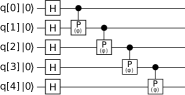
(a)

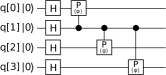
(b)

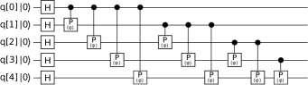
(c)

Figure 3: Quantum protocols for preparing graph states $\ket{\psi_{G}^{(1)}(\phi,0,\pi/2)}$ (15) (a), $\ket{\psi_{G}^{(2)}(\phi,0,\pi/2)}$ (16) (b), $\ket{\psi_{G}^{(3)}(\phi,0,\pi/2)}$ (17) (c).

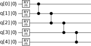
(a)

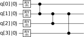
(b)

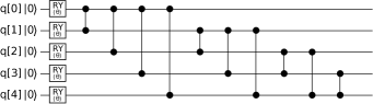
(c)

Figure 4: Quantum protocols for preparing graph states $\ket{\psi_{G}^{(1)}(\pi,0,\theta)}$ (15) (a), $\ket{\psi_{G}^{(2)}(\pi,0,\theta)}$ (16) (b), $\ket{\psi_{G}^{(3)}(\pi,0,\theta)}$ (17) (c).

We detect entanglement of qubits corresponding to vertices with degrees 1, 2, 3, 4 in graph states $\ket{\psi_{G}^{(1)}(\phi,0,\theta)}$ (15), $\ket{\psi_{G}^{(2)}(\phi,0,\theta)}$ (16), $\ket{\psi_{G}^{(3)}(\phi,0,\theta)}$ (17) on the quantum computer ibmq_athens. For this purpose the graph states have been prepared with quantum protocols presented in Figs. 3, 4 and the mean values $\braket{\sigma_{l}^{x}}$, $\braket{\sigma_{l}^{y}}$, $\braket{\sigma_{l}^{z}}$ have been measured using protocols presented in [9].

We quantify geometric measure of entanglement of qubit $q[0]$ corresponding to the vertex with degree 1 with other qubits in the states $\ket{\psi_{G}^{(1)}(\pi,0,\theta)}$, $\ket{\psi_{G}^{(1)}(\phi,0,\pi/2)}$ for different values of $\theta$ (see Fig. 5 (a)) and for different values of $\phi$ (see Fig. 6 (a)). In addition, the entanglement of the qubit $q[1]$ corresponding to the vertex with degree 2 was quantified in the states $\ket{\psi_{G}^{(1)}(\pi,0,\theta)}$, $\ket{\psi_{G}^{(1)}(\phi,0,\pi/2)}$ (see Fig. 5 (b), Fig. 6 (b)). In order to detect the geometric measure of entanglement of qubits represented by vertices with degrees 1 and 2 we choose qubits $q[0]$ and $q[1]$ because of small readout errors for these qubits in comparison with other qubits corresponding to vertices with the same degrees in the graph state $\ket{\psi_{G}^{(1)}(\phi,0,\theta)}$ (see Table 1).

Table 1: The calibration parameters of IBM’s quantum computer ibmq_athens on 9 June 2021 [41].

	$Q_{0}$	$Q_{1}$	$Q_{2}$
Readout error ($10^{-2}$)	1.07	1.30	1.70
Gate error ($10^{-4}$)	2.98	3.16	5.26
	$Q_{3}$	$Q_{4}$
Readout error ($10^{-2}$)	1.31	2.00
Gate error ($10^{-4}$)	2.54	2.89
CNOT error ($10^{-3}$)	CX0$\_$1	CX1$\_$0	CX1$\_$2
	12.04	12.04	11.13
	CX2$\_$1	CX2$\_$3	CX3$\_$2
	11.13	18.50	18.50
	CX3$\_$4	CX4$\_$3
	6.80	6.80

The geometric measure of entanglement of the qubit $q[1]$ corresponding to the vertex with degree 3 in the claw graph with other qubits in the states $\ket{\psi_{G}^{(2)}(\pi,0,\theta)}$, $\ket{\psi_{G}^{(2)}(\phi,0,\pi/2)}$ was also calculated (see Fig. 5 (c), Fig. 6 (c)). To quantify the geometric measure of entanglement in the case of $n_{l}=4$ graph states $\ket{\psi_{G}^{(3)}(\pi,0,\theta)}$, $\ket{\psi_{G}^{(3)}(\phi,0,\pi/2)}$ represented by the complete graph were prepared using protocols (see Fig. 3 (c), Fig. 4 (c)) and the geometric measure of entanglement of the qubit $q[0]$ with other qubits was quantified (see Fig. 5 (d), Fig. 6 (d)).

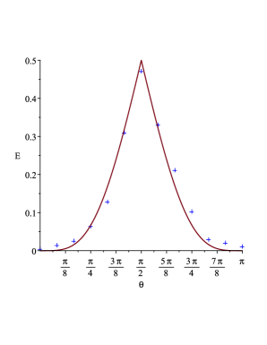
(a)

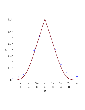
(b)

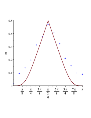
(c)

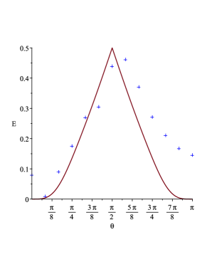
(d)

Figure 5: Results of detecting geometric measure of entanglement on ibmq_athens quantum computer (marked by crosses) and analytical results (line) for qubit q[0] (a) and qubit q[1] (b) with other qubits in state $\ket{\psi_{G}^{(1)}(\pi,0,\theta)}$ (15) for different values of $\theta$, for qubit q[1] with other qubits in state $\ket{\psi_{G}^{(2)}(\pi,0,\theta)}$ (16) (c) and for qubit q[0] with other qubits in state $\ket{\psi_{G}^{(3)}(\pi,0,\theta)}$ (17) (d) for different values of $\theta$.

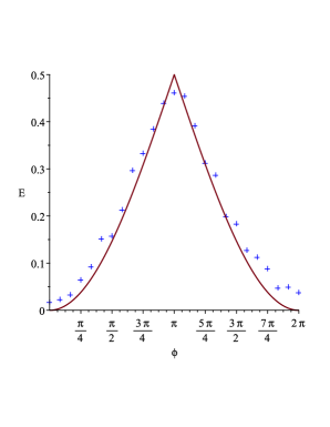
(a)

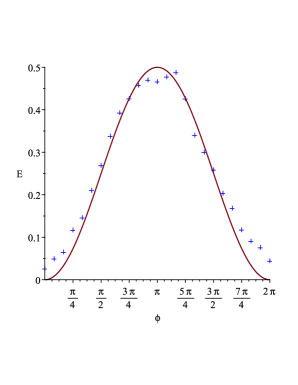
(b)

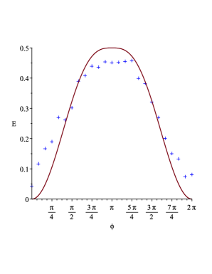
(c)

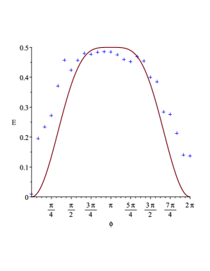
(d)

Figure 6: Results of detecting geometric measure of entanglement on ibmq_athens quantum computer (marked by crosses) and analytical results (line) for qubit q[0] (a) and qubit q[1] (b) with other qubits in state $\ket{\psi_{G}^{(1)}(\phi,0,\pi/2)}$ (15) for different values of $\phi$, for qubit q[1] with other qubits in state $\ket{\psi_{G}^{(2)}(\phi,0,\pi/2)}$ (16) (c) and for qubit q[0] with other qubits in state $\ket{\psi_{G}^{(3)}(\phi,0,\pi/2)}$ (17) (d) for different values of $\phi$.

The results for the geometric measure of entanglement obtained on the quantum computer for qubits in the graph states $\ket{\psi_{G}^{(1)}(\pi,0,\theta)}$, $\ket{\psi_{G}^{(1)}(\phi,0,\pi/2)}$ (see Fig. 5 (a), (b), Fig. 6 (a), (b)) are in good agreement with theoretical ones. In the case of graph states $\ket{\psi_{G}^{(2)}(\pi,0,\theta)}$, $\ket{\psi_{G}^{(2)}(\phi,0,\pi/2)}$, $\ket{\psi_{G}^{(3)}(\pi,0,\theta)}$, $\ket{\psi_{G}^{(3)}(\phi,0,\pi/2)}$ the results for the entanglement are not in so good agreement with analytical results because to prepare these states two-qubit gates have to be applied to qubits that are not connected directly according to connectivity map of IBM’s quantum computer ibmq_athens (see Fig. 1). Also, quantum protocols for preparing graph states represented by the complete graph (see Fig. 3 (c), Fig. 4 (c)) contain more gates than those for preparing graph states corresponding to the chain and the claw (see Fig. 3 (a), (b), Fig. 4 (a), (b)). This leads to accumulation of errors.

4 Conclusion

In the paper we have studied the geometric measure of entanglement of graph states generated by the action of controlled phase shift operators on a separable quantum state of the system, in which all the qubits are in arbitrary identical states (4). The expression for the geometric measure of entanglemet of a qubit with other qubits in graph state (4) represented by an arbitrary graph has been found (14). We have concluded that the entanglement depends on the absolute values of the parameter of the phase shift operator $\phi$ and the parameter $\theta$ of states (5) as well as on the degree of the vertex representing the qubit in the graph.

The geometric measure of entanglement has also been calculated on the 5-qubit IBM’s quantum computer ibmq_athens. Graph states corresponding to the graph with the structure of quantum computer ibmq_athens, the claw and the complete graphs have been prepared and the geometric measure of entanglement of qubits represented by vertices with degrees 1,2,3,4 has been found. Fixing parameter $\phi=\pi$ we have prepared graph states (15)-(17) and quantified their entanglement for different values of $\theta$ (see Fig. 5). In addition, we have set $\theta=\pi/2$ and examined dependence of the geometric measure of entanglement for different values of the parameter of the controlled phase gate $\phi$ in the case of graph states (15)-(17) (see Fig. 6). The results obtained with quantum calculations on the quantum device ibmq_athens are in good agreement with theoretical ones (see Figs. 5, 6).

5 Acknowledgments

The authors thank prof. Tkachuk V. M. for great support and useful comments during the research studies. This work was supported by Project 2020.02/0196 (No. 0120U104801) from National Research Foundation of Ukraine.

References

- [1] R. Horodecki, P. Horodecki, M. Horodecki, K. Horodecki, Rev. Mod. Phys. 81, 865 (2009).
- [2] A. Shimony, Ann. N.Y. Acad. Sci. 755, 675 (1995).
- [3] B. K. Behera, S. Seth, A. Das, P. K. Panigrahi, Quantum Information Processing 18, 108 (2019).
- [4] A. J. Scott, Phys. Rev. A 69, 052330 (2004).
- [5] P. Horodecki, A. Ekert Phys. Rev. Lett. 89, 127902 (2002).
- [6] J. Torrico, M. Rojas, S. M. de Souza, et al, EPL (Europhysics Letters), 108, 50007 (2014).
- [7] Yu-Bo Sheng, Lan Zhou, EPL (Europhysics Letters) 109, 40009 (2015).
- [8] A. M. Frydryszak, M. I. Samar, V. M. Tkachuk, Eur. Phys. J. D 71, 233 (2017).
- [9] A. R. Kuzmak, V. M. Tkachuk, Phys. Lett. A 384, 126579 (2020).
- [10] A. R. Kuzmak, V. M. Tkachuk, Condens. Matter Phys. 23, 43001 (2020).
- [11] Kh. P. Gnatenko, V. M. Tkachuk, Phys. Lett. A 396, 127248 (2021).
- [12] A. R. Kuzmak, V. M. Tkachuk, Eur. Phys. J. Plus 136, 564 (2021).
- [13] Yuanhao Wang, Ying Li, Zhang-qi Yin, Bei Zeng, npj Quant. Inf. 4, 46 (2018).
- [14] G. J. Mooney, Ch. D. Hill, L. C. L. Hollenberg, Sci. Rep. 9, 13465 (2019).
- [15] R. P. Feynman, Int. J. Theor. Phys. 21, 467 (1982).
- [16] C. H. Bennett, G. Brassard, C. Crepeau, R. Jozsa, A. Peres, W. K. Wootters, Phys. Rev. Lett. 70, 1895 (1993).
- [17] D. Bouwmeester, J.-W. Pan, K. Mattle, M. Eibl, H. Weinfurter, A. Zeilinger, Nature 390, 575 (1997).
- [18] A. K. Ekert, Phys. Rev. Lett., 67, 661 (1991).
- [19] R. Raussendorf, H. J. Briegel, Phys. Rev. Lett. 86, 5188 (2001).
- [20] S. Lloyd, Science 273, 1073 (1996).
- [21] I. Buluta, F. Nori, Science 326, 108 (2009).
- [22] Shaoping Shi, Long Tian, Yajun Wang et al, Phys. Rev. Lett. 125, 070502 (2020).
- [23] D. Llewellyn, Yu. Ding, I. I. Faruque et al, Nature Physics 16, 148 (2020).
- [24] Ni-Ni Huang, Wei-Hao Huang, Che-Ming Li, Scientific Reports 10, 3093 (2020).
- [25] Juan Yin, Yu-Huai Li, Sheng-Kai Liao et al, Nature 582, 501 (2020).
- [26] T. Jennewein, Ch. Simon, G. Weihs et al, Phys. Rev. Lett. 84, 4729 (2000).
- [27] A. Karlsson, M. Bourennane, Phys. Rev. A 58, 4394 (1998).
- [28] D. Schlingemann and R. F. Werner, Phys. Rev. A 65, 012308 (2001).
- [29] B. A. Bell, D. A. Herrera-Martí, M. S. Tame, Nature Communications 5, 3658 (2014).
- [30] P. Mazurek, M. Farkas, A. Grudka et al Phys. Rev. A 101, 042305 (2020).
- [31] D. Markham and B. C. Sanders, Phys. Rev. A 78, 042309 (2008).
- [32] Y. Qian, Z. Shen, G. He, and G. Zeng, Phys. Rev. A 86, 052333 (2012).
- [33] N. Shettell, D. Markham Phys. Rev. Lett. 124, 110502 (2020).
- [34] M. Hein, J. Eisert, H. J. Briegel, Phys. Rev. A 69, 062311 (2004).
- [35] O. Gühne, G. Tóth, Ph. Hyllus, H. J. Briegel, Phys. Rev. Lett. 95, 120405, (2005).
- [36] A. Cabello, A. J. Lopez-Tarrida, P. Moreno, J. R. Portillo Phys. Lett. A 373 2219 (2009).
- [37] Alba Cervera-Lierta J. I. Latorre, D. Goyeneche, Phys. Rev. A 100, 022342, (2019).
- [38] R. Mezher, J. Ghalbouni, J. Dgheim, D. Markham, Phys. Rev. A 97, 022333 (2018).
- [39] A. Akhound, S. Haddadi, Mohammad Ali Chaman Motlagh Mod. Phys. Lett. B 33, 1950118 (2019).
- [40] S. Haddadi, A. Akhound, Mohammad Ali Chaman Motlagh Int. J. Theor. Phys. 58, 3406 (2019).
- [41] IBM Q experience. https://quantum-computing.ibm.com/