Optimal Personalised Treatment Computation through In Silico Clinical Trials on Patient Digital Twins

Abstract

In Silico Clinical Trials, i.e., clinical experimental campaigns carried out by means of computer simulations, hold the promise to decrease time and cost for the safety and efficacy assessment of pharmacological treatments, reduce the need for animal and human testing, and enable precision medicine.

In this paper we present methods and an algorithm that, by means of extensive computer simulation–based experimental campaigns (ISCT) guided by intelligent search, optimise a pharmacological treatment for an individual patient (precision medicine). We show the effectiveness of our approach on a case study involving a real pharmacological treatment, namely the downregulation phase of a complex clinical protocol for assisted reproduction in humans.

1 Introduction

Model-based approaches to safety and efficacy assessment of pharmacological treatments (In Silico Clinical Trials, ISCT) hold the promise to decrease time and cost for the needed experimentations, reduce the need for animal and human testing, and enable precision medicine, where personalised treatments optimised for each patient can be designed before being actually administered. This is to be achieved by developing computational models for human physiology, patho-physiology, and drugs PharmacoKinetics (PK) and PharmacoDynamics (PD). Such computational models also define the possible physiological differences between different individuals and/or different reactions to drug administration. In particular, PK and PD models describe drug concentrations and effects over time in the human body (see, e.g., [2]), respectively.

Encapsulating knowledge of the human physiology into computational models is among the goals of Virtual Physiological Human (VPH) (see, e.g.,  [3]). Indeed, research in VPH provides mechanistic quantitative models of the human physiology at different levels of scale and for various medical areas (e.g.,  cardiology, endocrinology, oncology and neurology, see [4, 5, 6, 7, 8]). For example, several models have been proposed for molecules (e.g., [9]), cells (e.g., [10, 11]) and single organs (e.g., [12, 5, 13]). At upper levels in the hierarchy, we find models of human body compartments. Good examples are models in [14, 15, 16], which define the glucose regulation mechanism in patients with Type 1 Diabetes Mellitus, and the Hypothalamic–Pituitary–Gonadal (HPG) axis model presented in [6], which is specifically focused on hormones related to the human menstrual cycle. Finally, at the top level we find models of the whole human body, for example the Glucose-Insulin Model [17, 18], HumMod [19], and Physiomodel [20].

Independently of the level of scale used, most VPH models are defined by means of complex, highly non-linear differential equations. By means of numerical integration, such models can be executed within simulators in order to provide quantitative information about the time evolution of the modelled biological quantities (e.g., blood hormone or glucose concentrations).

VPH models at different positions in the above hierarchy are typically defined at different levels of abstraction. In order to find a trade-off between simulation accuracy and efficiency, multi-scale models can be built by integrating, interconnecting, and co-simulating models of the different organs or body compartments of interest, exploiting the different available levels of abstraction as required by the focus and scope of the in silico analysis to be performed.

Different languages are traditionally used to define VPH models. Among them are Systems Biology Markup Language (SBML) [21] and Physiological Hierarchy Markup Language (PHML) (see, e.g., [22]). The Modelica language (http://www.modelica.org), one of the most widely adopted open-standard general-purpose modelling languages for networks of dynamical systems within many areas of engineering, has been proposed as a common modelling platform for the integration of VPH, Pharmacokinetics/Pharmacodynamics (PKPD) models as well models for engineered systems such as biomedical devices (see, e.g., [23, 24]) in order to facilitate their co-simulation and analysis.

1.1 Motivations

Current pharmacological treatments are often designed with the average patient in mind. A key topic in precision medicine is to develop pharmacological treatments optimised for any given individual, namely personalised treatments (see, e.g., [25, 26]). Several optimisation criteria can be defined. A typical criterion is the minimisation of the overall amount of drug used, which often also reduces the probability of adverse side-effects and contributes to decrease the treatment cost.

With their amenability to define different individuals, VPH models of proved accuracy are a key enabler for precision medicine.

1.2 Contributions

In this paper we present methods and an algorithm that, by means of extensive computer simulation–based experimental campaigns (In Silico Clinical Trials, ISCT) guided by intelligent search, optimise a pharmacological treatment for an individual patient. We show the effectiveness of our approach on a case study involving a real pharmacological treatment, namely the downregulation phase of a complex clinical protocol for assisted reproduction in humans.

To do this, we exploit a state-of-the-art VPH model of the HPG axis (whose accuracy has been experimentally assessed in [6]) in order to conduct an ISCT. Namely, starting from clinical data collected from a real patient, we first compute her digital twin, which defines a digital representation of that patient physiology. Then, we compute in silico, by means of intelligent search on such a digital twin, the lightest (in terms of overall amount of administered drug) treatment still effective for that patient.

Our search algorithm extends standard artificial intelligence techniques (such as, e.g., classical planning [27], CSP [28] and SAT [29]) in order to intelligently explore the space of possible time-series of drug administrations (treatments) by driving a simulator of the VPH model at hand. To improve the performance of our search algorithm, we also define suitable ordering heuristics (which keep our approach complete) and we evaluate their marginal performance gain. Moreover, our implementation can be easily adapted to several VPH models and to a wide class of clinical treatments as it drives a Modelica black-box simulator.

In order to assess the technical viability of our approach, we exploit the above HPG axis VPH model to conduct a multi-arm ISCT involving $21$ patients (for which we have retrospective clinical measurements). For each such patient, who defines a distinct arm of our ISCT, we compute the optimal (lightest) still-effective downregulation treatment. Given that the required computation is extremely intensive, we conduct our ISCT on a large High Performance Computing (HPC) infrastructure.

The possibility to optimise in silico a complex treatment for a given human patient before its actual administration shows the potential of artificial intelligence search methods for model-based (in silico) medicine.

Paper outline

The paper is organised as follows. Section 2 describes some background knowledge, introduces the HPG axis model used in our case study and its phenotypes, defines the concept of clinical record and that of digital twin of a human patient. Section 3 describes the treatment we used as our case study. In Section 4 we describe our algorithm to find optimal personalised treatments by means of intelligent search which drives a black-box simulator of a patient digital twin. Section 5 describes our experimental campaign on retrospective data and analyses the outcome of our multi-arm ISCT. Finally, Section 6 discusses related work and Section 7 draws conclusions.

2 Formal framework

In this section we give the necessary background knowledge. We denote with $\mathbb{R}$, $\mathbb{R}_{0+}$, $\mathbb{R}_{+}$, $\mathbb{N}$, and $\mathbb{N}_{+}$ the sets of, respectively, all real, non-negative real, strictly positive real, non negative, and strictly positive integer numbers. Given $n\in\mathbb{N}_{+}$, we denote by $[n]$ the set of integers $\left\{1,\ldots,n\right\}$.

2.1 Virtual Physiological Human models

VPH models usually are hybrid systems defined by means of Ordinary Differential Equations (see, e.g., [30, 31, 32, 33]) as stated in Definition 2.1.

Definition 2.1

ODEA parametric ODE dynamical system is defined by a set of differential equations over time (variable $t\in\mathbb{R}_{0+}$) having the following form:

$$\dot{\mathbf{x}}(t)=\mathbf{f}(\mathbf{x}(t),\mathbf{u}(t),\lambda)$$

where:

• $\mathbf{x}(t)\in\mathbb{R}^{n_{x}}$ is called state vector, and models biological quantities;

• $\mathbf{u}(t)\in\mathbb{R}^{n_{u}}$ is called input vector, and models exogenous inputs (e.g., sequences of drug administrations);

• $\Lambda\subseteq\mathbb{R}^{n_{\lambda}}$ is called parameter space and $\lambda\in\Lambda$ denotes a parameter vector;

• $\mathbf{f}$ is a vector of functions defining system dynamics.

Above, we have $n_{x},n_{u},n_{\lambda}\in\mathbb{N}_{+}$.

In our setting, administrations of $n_{u}$ different pharmaceutical drugs (clinical actions) define inputs to the VPH model. Indeed, for each $i\in[n_{u}]$, the $i$-th component $u_{i}$ of the input vector $\mathbf{u}$ defines a function that associates to each time instant $t\in\mathbb{R}_{0+}$ the administered dose of the $i$-th drug, to be chosen within a set $A_{i}$ of possible doses (which always includes dose zero).

Given an assignment $\lambda$ to the VPH model parameters and an input vector $\mathbf{u}$ (i.e., a time sequence of administrations of the $n_{u}$ drugs defined within the model), the associated VPH model trajectory is a continuous-time function $\mathbf{x}_{\lambda}(t)$ (or, to simplify notation, $\mathbf{x}(\lambda,t)$) representing the time evolution of the biological quantities defined by the model when fed with $\mathbf{u}$ starting from its initial state and with its parameters set to $\lambda$. Of course, as the VPH model is causal, its trajectories up to any time point $\overline{t}\in\mathbb{R}_{0+}$ only depend on the restriction of the input up to time point $\overline{t}$ (see, e.g., [30, 34]).

2.2 The GynCycle Virtual Physiological Human model

In this section we describe the GynCycle VPH model, presented and evaluated in [6], which we will use as our case study.

GynCycle is an ODE-based model of the human female HPG axis, with a special focus on the interactions and feedback mechanisms between hormones like Gonadotropin-Releasing Hormone (GnRH), Follicle-Stimulating Hormone (FSH), Luteinizing Hormone (LH), Estradiol (E2), Progesterone (P4), Inhibin A (IhA), and Inhibin B (IhB) during the different stages of the menstrual cycle.

The model defines the time evolution of overall $33$ biological quantities (mostly blood concentration of hormones) and the PKPD of several pharmaceutical drugs used in assisted reproduction (in particular, we will focus on GnRH analogues like Triptorelin) by means of highly non-linear differential equations.

For example, equations defining the time evolution of LH, and FSH are as follows:

$$\dot{\text{LH}}_{\mathit{blood}}(t) =\frac{\text{LH}_{\mathrm{pit}}(t)}{V_{\mathit{blood}}}\cdot\left(b^{\text{LH}}_{\mathit{Rel}}+k_{\text{G-R}}^{\text{LH}}\cdot H^{+}(\text{G-R}(t),T_{\text{G-R}}^{\text{LH}};n_{\text{G-R}}^{\text{LH}})\right)$$

$$-(k_{\mathit{on}}^{\text{LH}}\cdot\text{R}_{\text{LH}}(t)+k_{\mathit{cl}}^{\text{LH}})\cdot\text{LH}_{\mathit{blood}}(t)$$

$$\dot{\text{FSH}}_{\mathit{blood}}(t) =\frac{\text{FSH}_{\mathrm{pit}}(t)}{V_{\mathit{blood}}}\cdot\left(b^{\text{FSH}}_{\mathit{Rel}}+k_{\text{G-R}}^{\text{FSH}}\cdot H^{+}(\text{G-R}(t),T_{\text{G-R}}^{\text{FSH}};n_{\text{G-R}}^{\text{FSH}})\right)$$

$$-(k_{\mathit{on}}^{\text{FSH}}\cdot\text{R}_{\text{FSH}}(t)+k_{\mathit{cl}}^{\text{FSH}})\cdot\text{FSH}_{\mathit{blood}}(t)$$

In the differential equations above, $\text{LH}(t)$, $\text{FSH}(t)$ etc. denote biological species of interest (in the example, the blood concentration of LH and FSH, respectively), while $b^{\text{LH}}_{\mathit{Rel}}$, $k^{\text{LH}}_{\mathit{cl}}$, etc. denote model parameters.

As such, GynCycle is a hybrid system whose inputs represent drug administrations. As it happens with VPH models of practical interest as GynCycle, the number and complexity of their differential equations makes symbolic analysis (by, e.g., a model checker for hybrid systems) an unviable option. Indeed, the model can be simulated by means of numerical integration in order to compute the time evolution of the hormones of interest upon administration of a sequence of drug doses. Thus, GynCycle is used as an executable black-box model.

2.3 GynCycle Virtual Phenotypes

VPH models like GynCycle typically take into account inter-subject variability (i.e., the physiological differences among different individuals) by including suitable parameters in their equations (like $b^{\text{LH}}_{\mathit{Rel}}$ and $k^{\text{LH}}_{\mathit{cl}}$ mentioned above). Different value assignments to model parameters yield different model time evolutions and/or different reactions to drug administrations, thus defining different Virtual Phenotypes. Intuitively, each VP represents a class of indistinguishable (as long as the VPH model is concerned) patients. Computing a complete set of VPs for the model at hand is the starting point to obtain a representative population of virtual patients (hence, ideally showing all possible phenotypes). In turn, this is the key enabler to perform ISCT to assess, e.g., safety and/or efficacy of a pharmacological treatment.

Unfortunately, computing the complete set of VPs defined by a complex VPH model like GynCycle is all but easy from the computational point of view, and may require weeks of massive simulation on large HPC infrastructures. This is due to the hidden presence of inter-dependency constraints among elements of the parameter vector which are usually not explicitly known, and hence not modelled. By ignoring such constraints (which would happen by, e.g., choosing values for the parameter vector elements in a uninformed random way) would yield with high probability to model behaviours that violate the laws of biology (and hence such parameter assignments could not be regarded as VPs).

In [35, 36], a statistical model checking–based approach using intelligent global search heuristics has been discussed. Such a methodology enables the computation of a population of VPs (parameter assignments showing time evolutions compatible with the laws of biology) that is complete with respect to the used heuristics up to an arbitrarily high statistical confidence. This approach was recently generalised in [37], where it proved its effectiveness in computing a population of VPs for a VPH model of the glucose regulation system in patients with Type 1 Diabetes Mellitus.

In this paper, we conduct our ISCT starting from a population $\mathcal{P}$ of around ${10}^{7}$ VPs, extracted using the algorithm in [35, 36] from a huge search space of ${10}^{75}$ possible candidate parameter vector assignments (set $\Lambda$ in Definition 2.1). By exploiting model locality assumptions typically made on ODE-based VPH models (i.e., small changes in the model parameters are expected to yield small changes in the overall model trajectory), the domain of each of the $75$ dimensions of $\Lambda$ has been discretised into $10$ possible values (see [35] for an evaluation of the appropriateness of this choice). We then ran the parallel tool described in [36] with error threshold equal to $0.01$% and statistical confidence bound equal to $95$%. This means that, upon termination, we have $95$% confidence that the probability of finding new VPs by further searching is at most $0.01$%.

2.4 Clinical records

In order to compute personalised optimal treatments, we will start from clinical data collected from a human patient. Along the lines of [35], a clinical record $\mathcal{C}$ (Definition 2.2) consists of a sequence of measurements for all biological quantities of interest, where each measurement maps a time instant to a measured value.

Definition 2.2 (Clinical record)

Let $S_{1},\ldots,S_{p}$ be the biological quantities of interest. A patient clinical record, $\mathcal{C}$, is a tuple $(C_{1},\dots,C_{p})$, where each $C_{i}$ ($i\in[p]$) is a finite sequence of pairs $(t,v)$ (possibly empty) where $t\in\mathbb{R}_{0+}$ denotes a time instant and $v\in\mathbb{R}_{0+}$ is the measured value of biological quantity $S_{i}$.

In our case study (fertility treatments), clinical records of interest collect measurements for the main hormones involved in the human menstrual cycle, namely: LH, FSH, E2, and P4.

2.5 Digital twin of a human patient

To compute a personalised treatment for a human patient, we first need to compute a digital representation for her. This will be done by using clinical data (in the form of a clinical record $\mathcal{C}$, Definition 2.2) available from that patient in order to select, from our representative population of VPs, the subset of VPs that are compatible with (i.e., fit) such data.

To do so, we proceed as follows. Let $\mathcal{C}$ be a clinical record and $\lambda$ be a VP of our population. We define $\eta(\mathcal{C},\lambda)$ as the average (over all biological quantities $S_{i}$, $i\in[p]$) Mean Absolute Percentage Error (MAPE) between the clinical measurements of $S_{i}$ in $\mathcal{C}$ and time evolutions of $S_{i}$ in VP $\lambda$. Formally:

$$\eta(\mathcal{C},\lambda)~{}=~{}\frac{1}{p}\sum_{i=1}^{p}\frac{1}{\left|C_{i}\right|}\sum_{(t,v_{i})\in C_{i}}\left|\frac{v_{i}-x_{i}(\lambda,t)}{\zeta(v_{i})}\right|$$

where $\zeta(v_{i})$ is $v_{i}$ if $v_{i}\neq 0$ and a small positive constant otherwise (to avoid division by zero).

By using such a metric, Definition 2.3 defines the concept of patient digital twin as the set of all VPs $\lambda$ in our population $\mathcal{P}$ having a value for $\eta(\mathcal{C},\lambda)$ up to a given threshold.

Definition 2.3

Given a clinical record $\mathcal{C}$, our complete population of VPs $\mathcal{P}$, a threshold $\delta\in\mathbb{R}_{0+}$ for our error metric $\eta$, the digital twin $P$ of $\mathcal{C}$ is the following set:

$$P(\mathcal{C})=\left\{\lambda\in\mathcal{P}~{}\middle|~{}\eta(\mathcal{C},\lambda)\leq\delta\right\}.$$

Intuitively, the digital twin of a human patient is a digital representation of the patient physiology in the form of all VPs entailing model behaviours that fit the patient clinical measurements (up to an average MAPE $\delta$).

3 Case study: downregulation in assisted reproduction treatments

In this section we define the treatment we used as our case study: the downregulation phase of an assisted reproduction protocol currently administered at the Department of Reproductive Endocrinology of University Hospital Zurich.

At each menstrual cycle of a human female, among the several follicles initially present in the ovaries, only one, unless in exceptional cases, grows and reaches maturity. A complex competition among follicles takes place, driven by a hormone-based feedback loop, in order to inhibit the maturation of multiple follicles.

An assisted reproduction treatment aims at neutralising (through drugs) such a feedback loop (downregulation phase), in order to achieve a controlled and an as-simultaneous-as-possible growth of $5$–$15$ ovarian follicles (stimulation phase). When the first three follicles reach a size where a mature oocyte (i.e., an egg cell ready for fertilisation) can be expected (about $18$ mm in diameter), ovulation is induced. Then, the oocytes are retrieved, those which are mature are tried to be fertilised in vitro, and implanted either immediately within the treatment cycle or later after cryopreservation (i.e., a preservation process by cooling) back into the uterus.

Assisted reproduction treatments are complex and challenging, with low average success rates (around $30$%) even in the top clinics, and with many factors that, to date, can be hardly kept under full control. Indeed, as hormonal regulatory systems occur within a complex network of endocrinological, neurological and psychological factors [38, 39, 40], they are difficult to capture within clinical studies, and model-based approaches might be of great aid in taking these many factors under better control.

Our case study is one of the worldwide classically used downregulation protocols aiming at suppressing the usual hormonal oscillations of the menstrual cycle (as in Figure 1) and preparing the patient to the following stimulation.

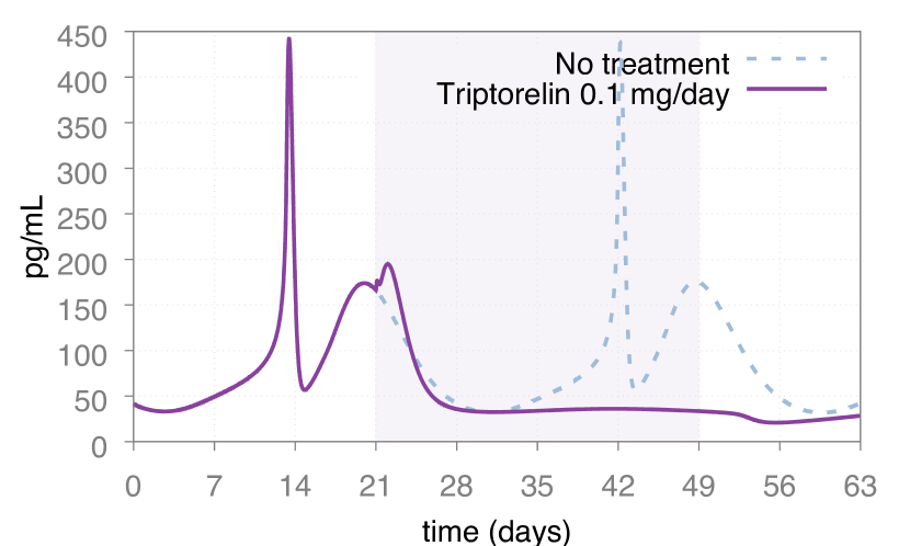
(a) E2

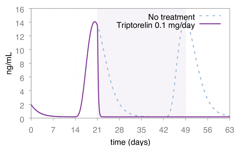
(b) P4

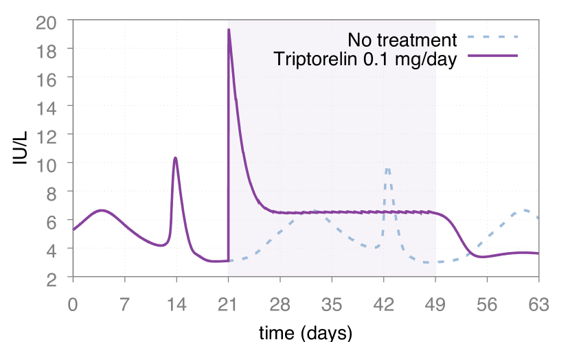
(c) FSH

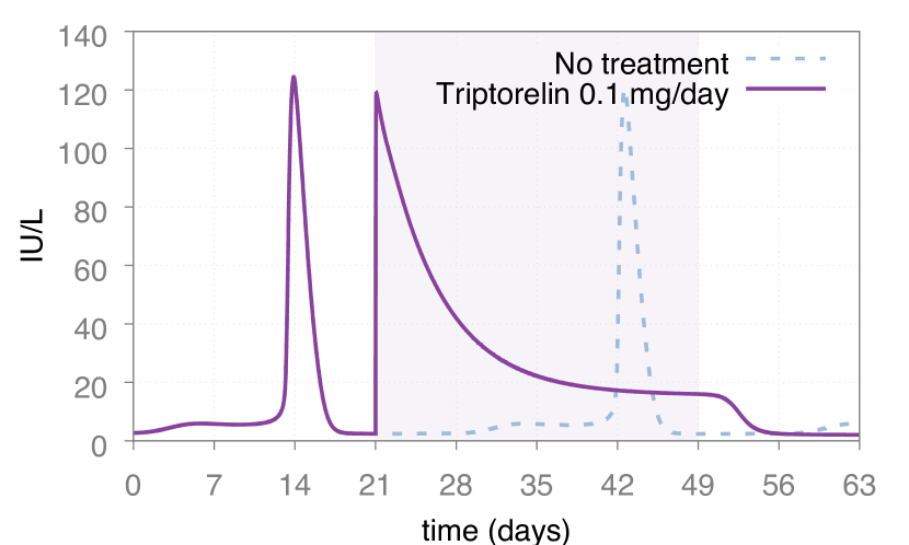
(d) LH

Figure 1: Expected downregulation effects on some of the hormones playing a role in the human female menstrual cycle. The coloured area defines the time window during which Triptorelin is administered.

At the Department of Reproductive Endocrinology of University Hospital Zurich, this protocol currently consists of a sequence of daily administrations of $0.1$ mg of Triptorelin, a GnRH analogue. For physiological reasons, downregulation is started within a precise time window of the menstrual cycle, namely between day $21$ and day $25$. The treatment might have different duration in order to address different patient reactions. In particular, a downregulation treatment is considered successful (effective) for a patient in case the blood concentrations of a given set of hormones and other physiological quantities go below certain thresholds within 9 days from the first drug administration, and stay always below such thresholds for the following $21$ days. As a consequence, a downregulation treatment might last up to $30$ days.

4 Computing optimal personalised treatments

In this section, we define the conditions of a successful treatment through invariants and goals (Section 4.1), describe how to perform digital twin simulations (Section 4.2), and describe the algorithm used at the core of our optimal personalised treatment computation (Section 4.3).

4.1 Modelling treatment invariants and goals

We define conditions that must be always and eventually satisfied by a successful treatment by means of invariants and goals, respectively. Invariant and goal treatment conditions are modelled as continuous-time monitors embedded within the VPH model, along the lines of [41, 42]. Monitors observe the state of the system and check whether the properties of interest are satisfied.

In particular, given a model trajectory $\mathbf{x}(\lambda,t)$ under a given input $\mathbf{u}$, our monitor output is Undet as long as $\mathbf{x}(\lambda,t)$ satisfies the invariants (in other words, the monitor decision is “undetermined” as long as there is hope to extend the current treatment into a successful treatment) and goes to and stays at value Fail as soon as invariants are violated. When a Undet model trajectory satisfies the goal conditions, the monitor output turns to Success, informing the caller that the input $\mathbf{u}(t)$ defines a successful treatment (i.e., an effective treatment which always satisfies invariants).

The use of continuous-time monitors embedded in the VPH model gives us a flexible way to model both bounded safety and bounded liveness properties, and is a standard approach in the simulation-based verification of cyber-physical systems (see, e.g., [43, 44]).

In our case study, the properties of interest are the conditions of successful downregulation treatments (Section 3). In particular, our invariant requires that the day of the first drug administration is between day $21$ and day $25$ of the menstrual cycle. Moreover, the value of all the biological quantities under observation must go and stay below their thresholds from the $9$-th day after the first drug administration. Our goal condition instead requires that values for those quantities stay below their thresholds for $21$ consecutive days.

As a consequence, our monitor output is Undet in the initial state, and eventually turns either to Fail or to Success (see Figure 2). Model output turns to value Fail as soon as, from the $9$-th day after the first drug administration, the value of any of the physiological quantities under observation exceeds its threshold. Conversely, model output turns from value Undet to value Success as soon as all the thresholds are satisfied for $21$ consecutive days.

Figure 2: Treatment monitor.

4.2 Digital Twin simulation

As anticipated in Section 2, the complexity of the (highly non-linear) differential equations typically occurring in actual VPH models hinders the possibility for their symbolic analysis. Numerical simulation is often the only means to compute the time evolution of the model quantities of interests (mainly blood hormone concentrations in our case study GynCycle model) upon a sequence of clinical actions (administration of one or more drugs with their associated doses). Also, as VPH model equations are often stiff, simulation can be an expensive process from a computational point of view.

Our algorithm for optimal personalised treatment computation regards the input VPH model as an executable black-box model. In order to drive the VPH model simulator, our algorithm assumes that it accepts the following basic commands (which are available or can be readily implemented within most modern simulators [45, 46]): store, load, free, run, get. Command $\texttt{store}(l)$ stores in memory the current state of the simulator and labels with $l$ such a state. Command $\texttt{load}(l)$ loads into the simulator the stored state labelled with $l$. Command $\texttt{free}(l)$ removes from the memory the state labelled with $l$. Command $\texttt{run}(a,t)$ (with $a\in A_{1}\times\cdots\times A_{n_{u}}$ and $t\in\mathbb{R}_{+}$) executes clinical action $a$ (thus administering given –possibly zero– doses for all available drugs) and then advances the simulation of time $t$. Command $\texttt{get}(x)$ (with $x$ denoting one of the model variables) returns the value of model variable $x$ in the current state.

Since the input of our algorithm is a digital twin $P(\mathcal{C})$ computed from a patient clinical record $\mathcal{C}$ and consisting of a set of $n_{p}\in\mathbb{N}_{+}$ VPs (see Section 2.5), during the search we drive the simulation of $n_{p}$ independent copies of our VPH model (each one connected to a copy of the monitor checking for treatment invariants and goals, as explained in Section 4.1). The different model copies are instantiated with different values for the model parameter vector defined in $P(\mathcal{C})$, hence represent the different VPs in the patient digital twin.

By means of commands $\texttt{run}(a,t)$ ($a\in A_{1}\times\cdots\times A_{n_{u}}$), we simultaneously apply the same clinical action to all VPs in $P(\mathcal{C})$ and synchronously advance all models by time $t$. Furthermore, by means of store and load commands, we can efficiently expand a tree of sequences of clinical actions, as typically done by backtracking-based state exploration algorithms. In particular, upon a backtrack, we only need to load back a previously stored state of our models, thus avoiding to simulate the entire input sequence starting from the initial state.

4.3 Intelligent backtracking–driven simulation

In this section we describe our intelligent search that drives a digital twin simulator, by defining our search tree (Section 4.3.1) and criteria for the evaluation and expansion of search tree nodes (Section 4.3.2). We also introduce two ordering heuristics aiming at efficiently pruning the search tree (Section 4.3.4) and speeding up the digital twin simulation time (Section 4.3.5), while retaining completeness of the overall algorithm.

4.3.1 Search tree definition

Given a patient clinical record $\mathcal{C}$, its digital twin $P(\mathcal{C})$, and possible alternative doses for each treatment drug at hand (i.e., sets $A_{1},\ldots,A_{n_{u}}$, each one including dose zero), our backtracking-based algorithm performs a search in the space of possible treatments (i.e., time sequences of clinical actions in $A_{1}\times\cdots\times A_{n_{u}}$). Under the following assumptions: (i) the sets of allowed doses $A_{1},\ldots,A_{n_{u}}$ for the $n_{u}$ drugs are finite; (ii) drug administrations occur at time instants multiple of a given time-quantum $\tau\in\mathbb{R}_{+}$; and (iii) sought treatments have a bounded duration ($\tau h$, with $h\in\mathbb{N}_{+}$ being the treatment horizon), we can limit our search to a finite tree of maximum depth $h$, where each tree node at depth $0\leq l\leq h$ defines a discrete sequence of $l$ clinical actions (elements of $A_{1},\ldots,A_{n_{u}}$), each one occurring in the first $l$ time points multiple of $\tau$.

As described in Section 4.2, our search algorithm drives a simulator containing multiple copies of the VPH model (one per VP in the digital twin given as input), each one connected to a copy of the monitor which checks for treatment invariants and goals.

Accordingly, each node of our search tree keeps also track of the digital twin simulator state reached by injecting the clinical action sequence of that node. This is done via a store command (see Section 4.2). A transition between a parent node and a child node consists of extending the clinical action sequence of the parent node with a new action $a\in A_{1}\times\cdots\times A_{n_{u}}$. In doing so, we also advance the digital twin simulator state of the parent node via a run command (see Section 4.2). In Section 4.3.2, we describe more in details how a search tree node is evaluated and expanded.

Before the search starts, for each VP $\lambda$ in the input digital twin, we prepare its associated copy of the VPH+monitor model within the digital twin simulator, by setting the parameter vector to $\lambda$. We also store the initial simulator state via a store command (see Section 4.2).

Clearly, the assumptions above together with the entailed search tree structure hold for a very wide class of treatments. For example, in our downregulation treatment case study, there is only one possible drug, namely Triptorelin, hence $n_{u}=$1$$. Also, as such treatments allow at most one Triptorelin administration per day, we can safely set $\tau=\text{1 day}$. Finally, successful treatments cannot last more than $h=$25$+$9$+$21$=$55$$ days, starting from day $1$ of the patient menstrual cycle (i.e., the latest cycle day, $25$, when the treatment might start, plus the latest day, 9, within which the safety conditions must be met, plus the number of consecutive days, $21$, in which the safety conditions must be always satisfied in order to declare success).

Moreover, in our case study, the initial simulator state represents day $1$ of the menstrual cycle of all VPs in the input digital twin.

4.3.2 Search tree node evaluation and expansion

At each node of the search tree, our algorithm needs to extend the current sequence of clinical actions (a treatment prefix, which is the empty sequence in the initial state). To do so, the algorithm:

1. Stores the current states of the VP models by means of a store command.

2. For each clinical action $a\in A_{1}\times\ldots\times A_{n_{u}}$ (according to the heuristic ordering discussed in Section 4.3.4), injects $a$ into the simulator and advances the simulation (simultaneously for all VPs defined within the simulator) by time $\tau$ (this is done by issuing a command $\texttt{run}(a,\tau)$).

3. If the monitor output for one VP returns Fail, the algorithm infers that there is no hope to extend the partial treatment to a complete treatment successful for all the VPs in the digital twin and issues a backtrack, by loading back (via a load command) the simulator state of all VPs associated to the parent node in the search tree.

4. Otherwise, if the monitor output for all VPs is Success, the algorithm infers that the current treatment is successful for all VPs.

5. Otherwise, the algorithm continues by expanding the new search tree node and extending the current treatment prefix.

Whenever no further actions can be executed in the current node of the search tree, the current simulator state is freed from memory by a free command before triggering a backtrack.

In order to reduce the required simulation time when expanding each node, the multiple model copies are not actually packaged into a single (much heavier to be simulated) model, but are kept separate and simulated sequentially. This allows our algorithm to perform two performance optimisations: a sort of early pruning of the current treatment prefix and a dynamic revision of the order with which the VPs in the input digital twin will be actually simulated in the sequel (Section 4.3.5).

4.3.3 Optimality constraint

Since we seek the optimal personalised treatment for the input digital twin, our algorithm does not stop at the first found successful treatment. Indeed, along the lines of [47], it keeps track of the lightest successful treatment found so far, i.e., the one envisioning the administration of the minimum overall drug amount $D_{\text{min}}\in\mathbb{R}_{0+}$. Initially, $D_{\text{min}}$ is set to $+\infty$.

At each node of the search tree, any action extending the current partial treatment with an administration of a drug dose which would make the overall administered drug amount reaching or exceeding $D_{\text{min}}$ is regarded as not applicable.

The optimality constraint (whose threshold is updated each time a new optimal treatment is found), the presence of a bounded horizon $h$ and the fact that our algorithm does not stop at the first successful treatment clearly guarantee that a global optimum is always returned (if any successful treatment exists).

4.3.4 Action ordering heuristic

In a black-box setting as ours, no inference can be made on the effects of each candidate action without performing a simulator run to actually advance the model and then querying the model monitor output. Hence, approaches to compute, through inference, a dynamic preference order among the candidate actions to be tried during search (as those exploited in, e.g., classical planning, planning for white-box hybrid systems –see Section 6– or (Q)CSP, SAT or local search solvers, see e.g., [28, 29, 48, 49, 50, 51, 52]) cannot be applied.

The only information available to the algorithm without running the simulator is value $D_{\text{min}}$ and the overall cost of the current partial treatment (overall amount of drug administered). Hence, given that our algorithm searches for a successful treatment of minimum cost and that any action has a non-negative contribution to the overall treatment cost, not surprisingly tries the clinical actions on each node in the search tree in ascending order of their associated dose (i.e., cost), hence performing a greedy, optimistic choice.

4.3.5 Dynamic VP simulation ordering

When, during the evaluation of search tree node, the monitor output after the simulation of a VP in the digital twin returns Fail, our algorithm, by performing a sort of early pruning, does not simulate nor evaluate the remaining VPs, but it backtracks and tries the next available action from the parent node, if any. Upon backtracking, the algorithm changes the verification ordering of the VPs in the digital twin in such a way that those VPs not satisfying treatment invariants or not yet simulated in the previous search step are simulated first. The rationale is that those VPs that already satisfied treatment invariants in previous step, will more likely satisfy treatment invariants in the current step, where a slightly different drug dose is chosen.

5 Multi-arm In Silico Clinical Trial

In this section we outline how we set up and conducted our ISCT in order to assess the technical viability of the proposed approach.

5.1 Retrospective clinical records

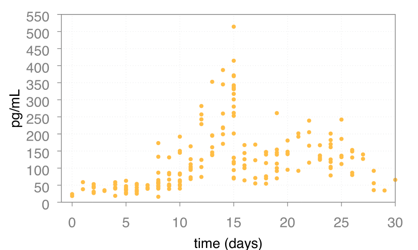
(a) E2

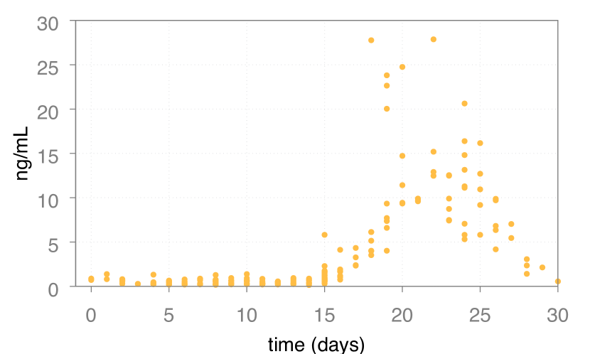
(b) P4

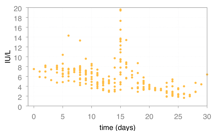
(c) FSH

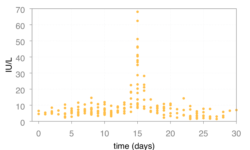
(d) LH

Figure 3: Measurements (dots) of, respectively, E2, P4, FSH and LH of the $21$ clinical records within the dataset from Pfizer Inc. and Hannover Medical School (Germany).

Our ISCT has been conducted against retrospective clinical data courtesy of Pfizer Inc. and Hannover Medical School (Germany).

In particular, such our overall dataset consists of $21$ patient clinical records for a total of around $800$ measurements. Each clinical record comprises measurements for the hormones that play the most important role during the human menstrual cycle: LH, FSH, E2, and P4. Figure 3 shows measurements of such hormones in our overall dataset.

Each of the $21$ clinical records in our retrospective clinical data defines a distinct arm of our multi-arm ISCT.

5.2 Computing digital twins: exclusion criteria and VP selection

From the GynCycle model, we generated a population $\mathcal{P}$ of around ${10}^{7}$ VPs as explained in [35, 36] and recapped in Section 2.3. Hence, such a population is representative of (almost) all patient behaviours allowed by the model (in the sense of [35, 36]). Note that, although generating such a population required weeks of HPC computation, this is a one-time task for each VPH model.

In order to carry out our multi-arm ISCT, we computed a digital twin for each of the $21$ clinical records in our retrospective clinical data. In particular, we set the threshold value $\delta$ (Definition 2.3) to $35$% and, for each clinical record $\mathcal{C}$, we included in the digital twin of $\mathcal{C}$, $P(\mathcal{C})$, all $\lambda\in\mathcal{P}$ such that $\eta(\mathcal{C},\lambda)\leq$35$\%$. Hence, for each clinical record, we selected all VPs having an average MAPE at most $35$%.

Since the reference downregulation treatment of Section 3 does not succeed on all possible phenotypes (this is not surprising since, as described in Section 3, fertility treatments are known to have a low rate of success), we removed from $P(\mathcal{C})$ those VPs for which the treatment using the maximum allowed dose (i.e., $0.1$ mg on each day for up to $30$ days, see Section 3) fails, for any $\mathcal{C}$. Such an exclusion criterion directly stems from domain knowledge on downregulation treatments (namely: for these protocols, if a treatment envisioning one full drug dose per day fails for a patient, a lighter treatment will fail as well). Our $21$ digital twins contain, on average, $843\,424$ VPs each.

Unfortunately, in the worst-case scenario, each step of our backtracking search requires to simulate all VPs within the input digital twin in order to check the monitor output (i.e., treatment invariants and goals, see Section 4.3.2). Thus, since simulating one VP requires seconds of numerical integration, the total computation time of our algorithm is highly affected by the size of the input digital twin, and may easily become impractical.

To overcome such an obstacle, we note that within a digital twin of a given clinical record we can (and typically do) have VPs exhibiting very similar model behaviours (both with and without drug administrations). Simulating such very similar VPs would then simply be a waste of computation as long as our ISCT is concerned. In order to reduce the size of a digital twin, we compute a subset $\hat{P}(\mathcal{C})$ of $P(\mathcal{C})$, for each given clinical record $\mathcal{C}$, such that $\hat{P}(\mathcal{C})$ does not contain such redundant VPs.

To do so, we define the distance among the time evolutions of any biological quantity $S_{i}$ ($i\in[n_{x}]$) of two VPs normalised against the time evolution of $S_{i}$ of a third (reference) VP (Definition 5.1).

Definition 5.1

Let $\lambda,\lambda^{\prime}$ and $\lambda^{\star}$ be three VPs of a VPH model defining $n_{x}$ biological quantities.

For every biological quantity $S_{i}$ ($i\in[n_{x}]$) the distance between $\lambda$ and $\lambda^{\prime}$ with respect to $\lambda^{\star}$ on $S_{i}$ is:

$$d_{i,\lambda^{\star}}(\lambda,\lambda^{\prime})=\frac{\sqrt{\int_{0}^{+\infty}{\left[x_{i}(\lambda,t)-x_{i}(\lambda^{\prime},t)\right]^{2}~{}\text{d}t}}}{\zeta\left(\sqrt{\int_{0}^{+\infty}{x_{i}(\lambda^{\star},t)^{2}~{}\text{d}t}}\right)}$$

where, as usual, $\zeta(\alpha)$ is $\alpha$ when $\alpha\neq$0$$ and a small constant otherwise (in order to avoid division by $0$).

Intuitively, Definition 5.1 defines the Euclidean distance between the time evolutions of biological quantity $S_{i}$ of two given VPs ($\lambda$ and $\lambda^{\prime}$) normalised with respect to the $L_{2}$-norm of that of a reference VP, $\lambda^{\star}$. In practice, we will compute the above distance using a bounded-horizon simulation, i.e., model trajectories will be defined for $0\leq t\leq h$, where $h$ is the treatment horizon. Hence, to match the above general definition, we assume that, for any $t>h$, $x_{i}(\lambda^{\star},t)$, $x_{i}(\lambda,t)$ and $x_{i}(\lambda^{\prime},t)$ are $0$.

Given this notion of distance, we build $\hat{P}(\mathcal{C})$ from the digital twin $P(\mathcal{C})$ of a clinical record $\mathcal{C}$ as follows:

• We select, from $P(\mathcal{C})$, the reference VP $\lambda^{\star}$ as one that minimises $\eta(\mathcal{C},\lambda^{\star})$. In other words, $\lambda^{\star}$ is one of the VPs of $\mathcal{P}$ that best matches the clinical measurements of $\mathcal{C}$.

• We remove from $P(\mathcal{C})$ those VPs whose time evolutions of all biological quantities have a distance below a certain threshold from other VPs in $\hat{P}(\mathcal{C})$ with respect to $\lambda^{\star}$ (Definition 5.2).

Such a distance threshold obviously depends on the VPH model and treatment subject of the ISCT.

Definition 5.2

Let $\mathcal{C}$ be a patient clinical record, $P(\mathcal{C})$ be its digital twin, $\lambda^{\star}$ be any VP such that $\eta(\mathcal{C},\lambda^{\star})$ is minimal, and $d$ be the distance function of Definition 5.1.

Then, given a threshold $\theta$, we call compact digital twin $\hat{P}(\mathcal{C})$ any subset of $P(\mathcal{C})$ such that the following condition holds:

$$\forall\lambda\in P(\mathcal{C})\>.\>\lambda\not\in\hat{P}(\mathcal{C})\rightarrow\exists\lambda^{\prime}\in\hat{P}(\mathcal{C})\>.\>\forall i\in[n_{x}]\>d_{i,\lambda^{\star}}(\lambda,\lambda^{\prime})\leq\theta/2.$$

As a result of the application of the above approach and of our exclusion criteria, we obtained compact digital twins with an average size of $11$. This has been achieved by tuning the distance threshold $\theta$ in such a way that: (i) VPs having redundant and undistinguishable behaviours have been filtered out; (ii) the computed compact digital twins were representative enough for all VPs in corresponding patient digital twins; and (iii) their sizes were small enough to be computationally affordable. Figure 4 shows the distribution of their sizes.

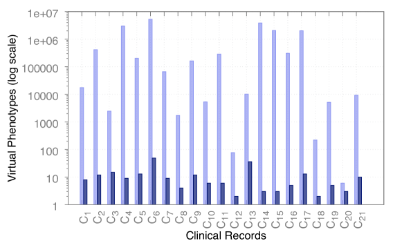
Figure 4: Bar chart showing digital twin sizes (in terms of number of VPs) before (light) and after (dark) the removal of redundant VPs and the application of our exclusion criteria for each clinical record.

5.3 Multi-arm In Silico Clinical Trial run

We ran our $21$-arm ISCT using a large HPC infrastructure (the Marconi cluster) kindly provided by the Cineca consortium.

For each patient clinical record $\mathcal{C}$ in our retrospective clinical data (see Section 2.4), we, first, computed a compact digital twin $\hat{P}(\mathcal{C})$ (see Section 5.2), and then we ran our algorithm of Section 4 on an independent node of the cluster searching for an optimal (i.e., lightest) and robust (with respect to all VPs of $\hat{P}(\mathcal{C})$) downregulation treatment for that specific digital twin. Thus, the whole $21$-arm ISCT has been conducted in an embarrassing parallel fashion.

Each VP in a compact digital twin has been encoded in a Modelica (http://www.modelica.org) model (encompassing the GynCycle VPH model taking clinical actions as input, a parameter vector assignment, and a monitor to check for treatment invariants and goals) and has been simulated using JModelica v2.1 (http://www.jmodelica.org). Our search algorithm (which drives a Modelica simulator per VP) has been implemented in Python.

In the following sections, we first evaluate the marginal impact of our heuristic ordering of actions (Section 5.3.1) and of our dynamic simulation ordering of VPs within a digital twin (Section 5.3.2). Then, we present computational results (Section 5.3.3) and outcomes (Section 5.3.4) of our multi-arm ISCT.

5.3.1 Evaluation of the action ordering heuristic

The goal of this section is to assess the marginal impact of the heuristic presented in Section 4.3.4, which sorts actions by their ascending associated cost (administered drug dose), in the overall efficiency of the optimal personalised treatment search algorithm.

To this end, we compare it against $10$ runs of an action selection strategy that evaluates the possible actions in random order when expanding each node of the search tree, and compare the performance of our heuristics against such reference strategy.

In particular, we defined a limit of ${10}^{4}$ on the number of search tree nodes to expand, and analysed how fast the cost (overall amount of drug dose) associated to the personalised treatments found decreases during the search space exploration, on all digital twins involved in our multi-arm ISCT.

In Figure 5, we present $3$ representative executions where our heuristic finds an optimal solution at different points in time (with respect to the number of expanded search tree nodes). For convenience of presentation, the initial value of $D_{min}$ in Figure 5 is set to $3.0$ (drug quantity employed by the reference treatment, i.e., $0.1$ mg on each day for up to $30$ days) instead of $+\infty$ (as stated in Section 4.3.3). This is in agreement with our exclusion criteria of Section 5.2 as the reference treatment succeed on all VPs within our digital twins.

We note that, by choosing actions randomly, the algorithm might show its first solution improvements a bit earlier (Figures 5(a) and 5(c)). However, in all cases, our heuristics finds the optimal solution (i.e., the lightest treatment) within a number of expanded nodes which is orders of magnitude lower than the number of expanded nodes required by the random action ordering strategy. As an example, Figure 5(c) shows that, after ${10}^{4}$ expanded nodes, $8$ out of $10$ runs with the random action ordering still failed to find a solution better than the reference treatment (i.e., $3.0$ mg).

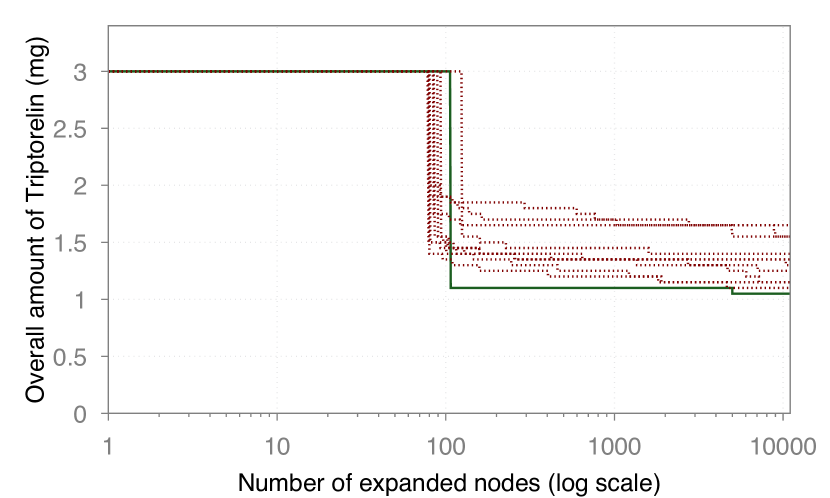
(a)

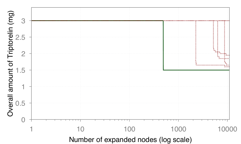
(b)

(c)

Figure 5: Comparison of solution paths traversed by our algorithm when using our ordering heuristic (green line) against the references (red dashed lines) among different digital twins of our multi-arm ISCT.

5.3.2 Evaluation of the dynamic ordering of VPs within a digital twin

In order to evaluate the marginal impact of our dynamic VP simulation order within the input digital twin (Section 4.3.5) at each search tree node, we compared the execution of our algorithm against a reference obtained by averaging $10$ different runs where the initial order of the VPs is randomised and fixed at the beginning of the search.

In particular, we ran our algorithm for each digital twin involved in our multi-arm ISCT, and compared the saving in terms of the number of simulations performed within each given number of search tree nodes.

Figure 6 shows our result on $3$ digital twins having different sizes: (i) a small size — $3$ VPs (Figure 6(a)); (ii) an average size — $13$ VPs (Figure 6(b)); and (iii) a large size — $36$ VPs(Figure 6(c)); which are representative of the spectrum of behaviours among our digital twins.

We note that the our dynamic VP simulation order is always beneficial. The highest saving in the number of simulations always occurs at the early stages of the search, where the most pruning activity is performed. In deeper stages of the search, the savings stabilise at values of the order of $10$%–$20$%. Since the time needed to simulate a VP is essentially constant (as VPs differ only in model parameter values and not in the system of Ordinary Differential Equations, ODEs), such savings translate in comparable reductions of the overall computation time. ODE

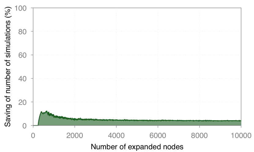
(a)

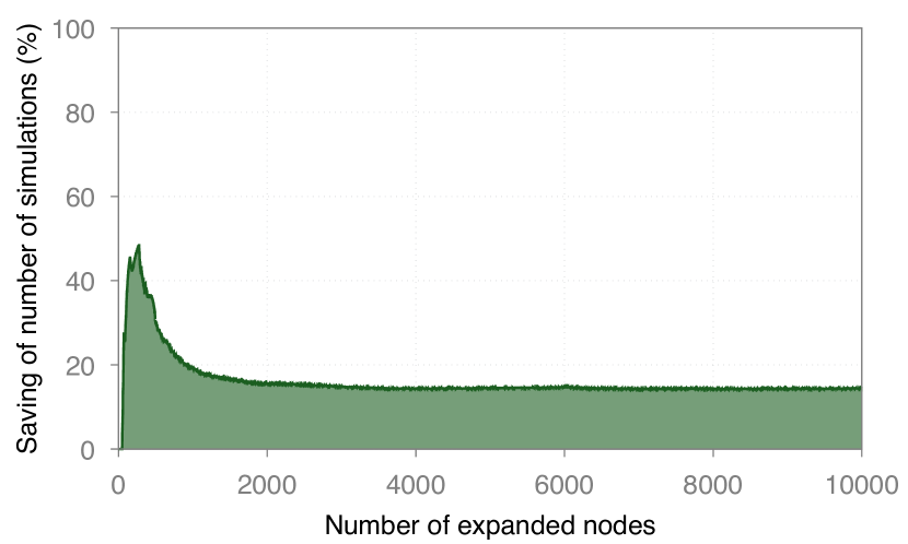
(b)

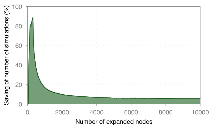
(c)

Figure 6: Marginal impact of our dynamic VP simulation ordering strategy among the digital twins of our multi-arm ISCT.

5.3.3 Computational results

We ran our multi-arm ISCT on the Marconi HPC infrastructure kindly provided by Cineca, Italy. Due to CPU-hours budget limit, we ran each arm of our ISCT in parallel for $15$ days. Each arm searches the optimal treatment for one of the $21$ patients in our dataset. Indeed, our algorithm can be regarded as an any-time algorithm in that, at any moment during search, it keeps track of the lightest successful treatment found so far.

Figure 7(a) gives, for each ISCT arm, the share of simulation time within the whole computation time. As we already argued in Section 5.2, the size of the input digital twin highly impacts the speed (in terms of expanded search tree nodes per seconds) of our algorithm. In fact, in each search node (in the worst case), our algorithm needs to numerically simulate all VPs within the input digital twin. As shown in Figure 7(a), the time spent in carrying out simulations is, on average, the $81.20$% of the total computation time.

This implies that any technique aimed at reducing the average number of simulations per search node (like the reduction of the size of the considered digital twin defined in Section 5.2, the action order heuristic evaluated in Section 5.3.1, and the dynamic VP simulation ordering evaluated in Section 5.3.2) is expected to have a substantial impact on the actual performance of the algorithm.

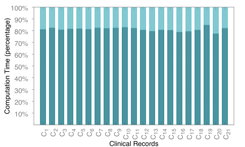
(a) Time share of digital twin simulations (dark bars) wrt. total computation time (dark and light bars)

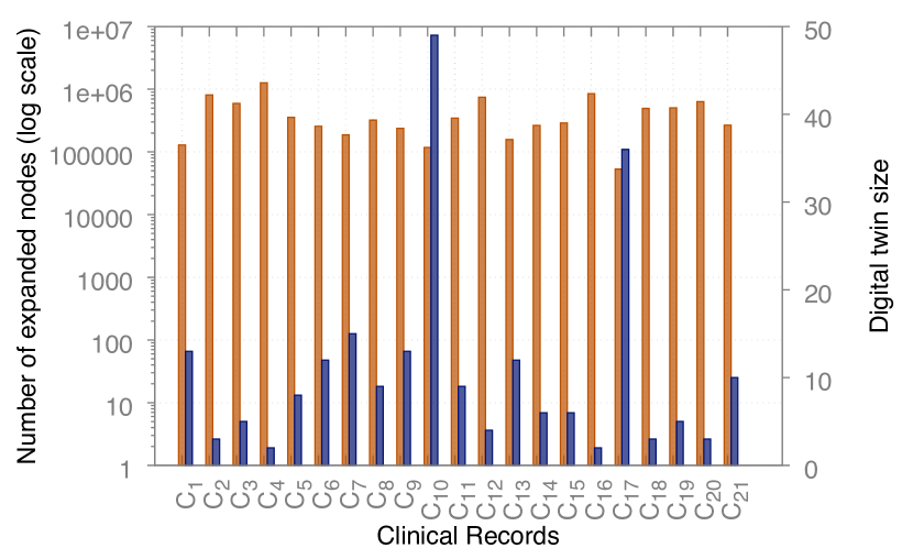
(b) Expanded search tree nodes (orange bars, left Y axis) vs. digital twin sizes (blue bars, right Y axis)

Figure 7: Computational results of our ISCT.

Figure 7(b) shows, for each of the $21$ parallel search processes (one per clinical record), the number of search nodes expanded within our time limit of $15$ days (orange bars, left Y axis), and compares it to the size of the digital twin considered for that clinical record (blue bars, right Y axis).

The figure show a clear negative correlation (correlation coefficient equal to $-60$%) between number of expanded nodes within our time limit and the digital twin size for all clinical records. For example, we note that when the digital twin size is small, as for, e.g., $\mathcal{C}_{4}$, the number of expanded nodes is large, i.e., near ${10}^{6}$. Instead, when the digital twin size is large, as for, e.g., $\mathcal{C}_{17}$, the number of expanded nodes is quite low, i.e., less than $3\text{\times}{10}^{4}$.

5.3.4 ISCT outcomes

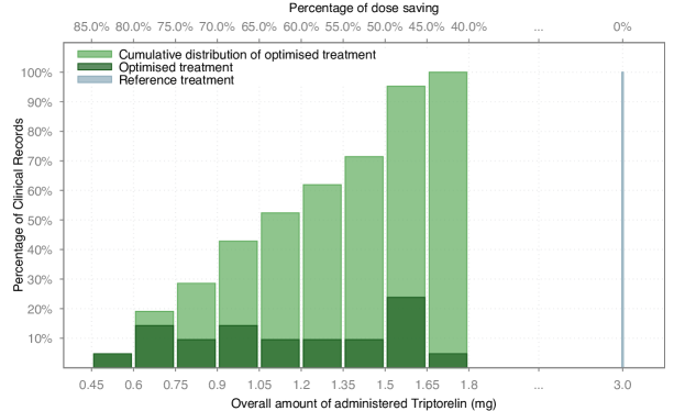
Figure 8: Multi-arm ISCT outcomes.

Figure 8 shows the distribution of the total amount of drug employed by the optimal personalised treatments computed by our algorithm. Note that, although we ran our multi-arm ISCT with a limited time budget and did not find provably lightest treatments, the treatments we actually computed use, on average, less than half ($40.82$%) of the drug quantity employed by the reference treatment of Section 3 (i.e., $0.1$ mg on each day for up to $30$ days, totalling up to $3$ mg and never less than $2.8$ mg, since the required thresholds are never reached before day $7$). As Figure 8 shows, the computed treatments save, on average, $59.18$% of the drug administered in the reference treatment (standard deviation: $13$%).

In Figure 9, we show our computed treatments for the $21$ patient clinical records during our multi-arm ISCT. We note that, the majority of the computed drug administration sequences is close to the reference downregulation treatment in terms of administration frequency and treatment duration, i.e., around $28$ days. Besides this, there are also few computed treatments having a very light overall amount of drug dose. This of course depends on the ability of the digital twins to capture patient peculiarities and in general on the ability of the VPH model at hand to represent the human physiology of interest.

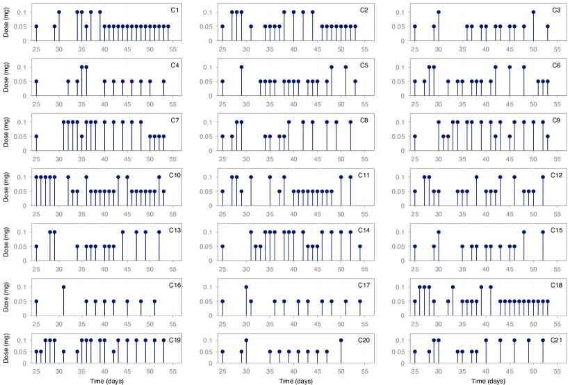
Figure 9: Personalised treatments computed through our multi-arm ISCT in $15$ days.

6 Related work

Individualised treatments have the potential value to reduce costs and improve outcomes of standard clinical treatments. In recent years data-driven techniques have been investigated thanks to the availability of big data [53]. For example, the knowledge-base approach in [54] has been used to optimise treatment plans for lung cancer. Unfortunately, in presence of scarce clinical data for the patient at hand, the above approaches cannot be applied. For example, in our case study hormones blood concentrations are not measured every day, since those measurements are costly and invasive.

Model-based approaches, exploiting PK, as e.g., [55], are used instead to build populations of virtual phenotypes. Such populations are used to optimise and individualise drug doses [56, 57]. PK-based models, however, do not define how administered drugs can affect a VP (namely, PharmacoDynamics, PD), i.e., possible side-effects due to drug administrations are not taken into account.

In our model-based setting, we have to face with complex VPH models, e.g., HumMod [19], Physiomodel [20], and GynCycle [6] defined through highly non-linear differential equations modelling the underlying biological mechanisms (e.g., inhibitory and stimulatory effects). As outlined in Section 2.1, such VPH models are hybrid systems that can be defined by systems of ODEs (see, e.g., [58, 32, 33]) whose inputs are discrete event sequences (see, e.g., [41, 44]). To find an optimal treatment means to find an optimal plan in hybrid domains, where the behaviour of the given system is described by both discrete and continuous quantities. In the literature, there are many techniques to model planning problems in hybrid domains, e.g., PDDL+ [59, 60]. Most of PDDL+ planners can deal only with linear dynamics (e.g., [61]). [62] proposed a Satisfiability Modulo Theories (SMT)-based approach for solving PDDL+ problems with non-linear dynamics. Model checking techniques are also used to find plans. Examples in this direction are [63, 64], which exploits symbolic model checking, UPMurphi [65, 66], which given as input a PDDL+ problem specification computes a universal plan, CGMurphi  [67], an explicit model checker used to compute optimal controllers, and [68, 69, 70, 71], which define methodologies to compute controllers for non-linear hybrid systems. However, as outlined in Section 4.2, the typical complexity of the differential equations of VPH models relevant for clinical practice makes such models out of reach for symbolic approaches like those mentioned above, and appoints numerical integration as the only viable means to compute (black-box) the model evolutions under a given input function.

In particular, even considering that clinical actions have constant and equal duration (as, e.g., in [72]), no reasoning or inference can be made on action effects in a black-box setting as ours, because the only way to interact with the models is through numerical simulation.

The automated synthesis of rational decisions and plans in black-box environments is common in several other application domains of high industrial relevance, like smart grids (see, e.g., [73, 74, 75]), games (see, e.g., [76]) and real-time manoeuvring of Unmanned Aerial Vehicles (see, e.g., [77]).

The works closest to ours are those in [76, 78] and citations thereof, where a simulator is used to discover the effect of actions. In such works, the simulator is defined as a factored state model where actions are (black-box) procedures and states are represented in terms of variables. Then an algorithm, namely, Iterated Width (IW), is typically employed. It consists of iteratively calling a breadth-first procedure, namely, $\texttt{IW}(i)$, with $i=1,2,3,\ldots$, until the problem is solved or $i$ becomes greater than the number of state variables (see, e.g., [79]). During each call to $\texttt{IW}(i)$, states are pruned accordingly to how novel they are. A state is novel if and only if values for at most $i$ state variables have not seen before. Authors point out that IW is efficient for the majority of classical planning problems where it is enough that $i=1,2$, i.e., actions change at most 2 state variables. However, in our setting, our simulator state consists of the union of all state vectors, i.e., $\mathbf{x}(t)$, of each VP+monitor within the input digital twin. Moreover, the most of variables within such state vectors consist of real-valued biological quantities. Also, we remind that the dynamics of such model are defined by means of ODEs. Hence, when we apply a clinical action (and simulate our digital twin) the vast majority of state variables change their value. In this setting, applying IW means nearly always to call only $\texttt{IW}(n)$, with $n$ the overall number of variable of our simulator state. This behaviour makes the pruning on which IW relies on quite ineffective as IW degenerates to prune truly duplicate states, which are also extremely rare as our variables are real valued. Note that, in order to increase pruning of duplicate states, one could think of simplifying the dynamics of the VPH model at hand (e.g., by discretising state variable domains). However, this is not a straightforward approach as it poses several questions about accuracy, credibility, and trust of the entailed model predictions, which have to be again experimentally assessed.

7 Conclusions

In this paper we presented methods and algorithms based on intelligent search aimed at synthesising optimal personalised treatments by means of ISCT, exploiting quantitative models of the physiology and drugs PKPD of interest, and clinical measurements on human patients from which we define their digital twins.

We applied our approach on a case study involving a complex state-of-the-art model of the human female HPG axis, in order to compute, for any given patient, a personalised treatment for the downregulation phase of an assisted reproduction protocol, which is effective on the patient at hand, but minimises the overall amount of drug used (hence, indirectly, the associated cost as well as likelihood and severity of adverse effects).

The possibility to optimise in silico, in a few weeks of computation on a HPC infrastructure, a complex treatment for a given human patient before its actual administration shows the potential of artificial intelligence for model-based (in silico) precision medicine. This however calls for trusted VPH models, which is currently one of the major obstacles for the uptake of ISCT in clinical practice.

Indeed, the results of our ISCT (conducted using a state-of-the-art validated VPH model as GynCycle) are extremely promising, but must be taken with care. In particular, an in vivo evaluation of the actual effectiveness of the personalised treatments generated by our algorithm is needed in order to assess the accuracy of GynCycle in predicting the patient reactions to non-standard drug dosing patterns, as those computed by our algorithm.

Acknowledgements

We are grateful to the co-authors of the preliminary work in [1].

This work was partially supported by the following research projects/grants: Sapienza University 2018 project RG11816436BD4F21 “Computing Complete Cohorts of Virtual Phenotypes for In Silico Clinical Trials and Model-Based Precision Medicine”; Italian Ministry of University & Research (MIUR) grant “Dipartimenti di Eccellenza 2018–2022” (Dept. Computer Science, Sapienza Univ. of Rome); EC FP7 project PAEON (Model Driven Computation of Treatments for Infertility Related Endocrinological Diseases, 600773); INdAM “GNCS Project 2019”; CINECA Class C ISCRA Project no. HP10CPJ9LW.

Clinical data used were gathered during a study conducted within EU FP7 Project PAEON. This study has been registered in clin.trial.gov (NCT02098668).

References

- [1] Mancini T, Mari F, Massini A, Melatti I, Salvo I, Sinisi S, Tronci E, Ehrig R, Röblitz S, Leeners B. Computing Personalised Treatments through In Silico Clinical Trials. A Case Study on Downregulation in Assisted Reproduction. In: Proceedings of 25th RCRA International Workshop on Experimental Evaluation of Algorithms for Solving Problems with Combinatorial Explosion (RCRA 2018), volume 2271 of CEUR Workshop Proceedings. CEUR-WS.org, 2018.
- [2] Mould D, Upton R. Basic Concepts in Population Modeling, Simulation, and Model-Based Drug Development. CPT: Pharmacometrics & Systems Pharmacology, 2012. 1(9):1–14.
- [3] Clapworthy G, Kohl P, Gregerson H, Thomas S, Viceconti M, Hose D, Pinney D, Fenner J, McCormack K, Lawford P, Van Sint Jan S, Waters S, Coveney P. Digital Human Modelling: A Global Vision and a European Perspective. In: Duffy V (ed.), Digital Human Modeling. Springer, Berlin, Heidelberg. ISBN 978-3-540-73321-8, 2007 pp. 549–558.
- [4] Trayanova N, Boyle P, Nikolov P. Personalized imaging and modeling strategies for arrhythmia prevention and therapy. Current Opinion in Biomedical Engineering, 2018. 5:21–28. 10.1016/j.cobme.2017.11.007.
- [5] Cox L, Loerakker S, Rutten M, De Mol B, Van De Vosse F. A Mathematical Model to Evaluate Control Strategies for Mechanical Circulatory Support. Artificial Organs, 2009. 33(8):593–603. 10.1111/j.1525-1594.2009.00755.x.
- [6] Röblitz S, Stötzel C, Deuflhard P, Jones H, Azulay DO, van der Graaf P, Martin S. A Mathematical Model of the Human Menstrual Cycle for the Administration of GnRH Analogues. Journal of Theoretical Biology, 2013. 321:8–27. http://dx.doi.org/10.1016/j.jtbi.2012.11.020.
- [7] Ribba B, Kaloshi G, Peyre M, Ricard D, Calvez V, Tod M, Čajavec-Bernard B, Idbaih A, Psimaras D, Dainese L, Pallud J, Cartalat-Carel S, Delattre JY, Honnorat J, Grenier E, Ducray F. A Tumor Growth Inhibition Model for Low-Grade Glioma Treated with Chemotherapy or Radiotherapy. Clinical Cancer Research, 2012. 18(18):5071–5080. 10.1158/1078-0432.CCR-12-0084.
- [8] Jackson P, Juliano J, Hawkins-Daarud A, Rockne R, Swanson K. Patient-Specific Mathematical Neuro-Oncology: Using a Simple Proliferation and Invasion Tumor Model to Inform Clinical Practice. Bulletin of Mathematical Biology, 2015. 77(5):846–856. 10.1007/s11538-015-0067-7.
- [9] Roy P, Roy K. Molecular docking and QSAR studies of aromatase inhibitor androstenedione derivatives. Journal of Pharmacy and Pharmacology, 2010. 62(12):1717–1728. 10.1111/j.2042-7158.2010.01154.x.
- [10] Bächler M, Menshykau D, De Geyter C, Iber D. Species-Specific Differences in Follicular Antral Sizes Result from Diffusion-Based Limitations on the Thickness of the Granulosa Cell Layer. Molecular Human Reproduction, 2014. 20(3):208–221. 10.1093/molehr/gat078.
- [11] Iarosz K, Borges F, Batista A, Baptista M, Siqueira R, Viana R, Lopes S. Mathematical model of brain tumour with glia–neuron interactions and chemotherapy treatment. Journal of Theoretical Biology, 2015. 368:113–121. 10.1016/j.jtbi.2015.01.006.
- [12] Yalcinkaya F, Kizilkaplan E, Erbas A. Mathematical modelling of human heart as a hydroelectromechanical system. In: Proceedings of 8th International Conference on Electrical and Electronics Engineering (ELECO 2013). IEEE, 2013 pp. 362–366. 10.1109/ELECO.2013.6713862.
- [13] Müller LO, Toro EF. A global multiscale mathematical model for the human circulation with emphasis on the venous system. International Journal for Numerical Methods in Biomedical Engineering, 2014. 30(7):681–725. 10.1002/cnm.2622.
- [14] Kanderian S, Weinzimer S, Voskanyan G, Steil G. Identification of Intraday Metabolic Profiles during Closed-Loop Glucose Control in Individuals with Type 1 Diabetes. Journal of Diabetes Science and Technology, 2009. 3:1047–1057. 10.1177/193229680900300508.
- [15] Herrero P, Georgiou P, Oliver N, Reddy M, Johnston D, Toumazou C. A Composite Model of Glucagon–Glucose Dynamics for In Silico Testing of Bihormonal Glucose Controllers. Journal of Diabetes Science and Technology, 2013. 7:941–951. 10.1177/193229681300700416.
- [16] Dalla Man C, Micheletto F, Lv D, Breton M, Kovatchev B, Cobelli C. The UVA/Padova Type 1 Diabetes Simulator: New Features. Journal of Diabetes Science and Technology, 2014. 8:26–34. 10.1177/1932296813514502.
- [17] Schaller S, Willmann S, Lippert J, Schaupp L, Pieber T, Schuppert A, Eissing T. A generic integrated physiologically based whole-body model of the glucose-insulin-glucagon regulatory system. CPT: Pharmacometrics & Systems Pharmacology, 2013. 2(8):1–10. 10.1038/psp.2013.40.
- [18] Schlender JF, Meyer M, Thelen K, Krauss M, Willmann S, Eissing T, Jaehde U. Development of a Whole-Body Physiologically Based Pharmacokinetic Approach to Assess the Pharmacokinetics of Drugs in Elderly Individuals. Clinical Pharmacokinetics, 2016. 55(12):1573–1589.
- [19] Hester R, Brown A, Husband L, Iliescu R, Pruett W, Summers R, Coleman T. HumMod: a modeling environment for the simulation of integrative human physiology. Frontiers in physiology, 2011. 2:12.
- [20] Mateják M, Kofránek J. Physiomodel – An integrative physiology in Modelica. In: Proceedings of 37th Annual International Conference of the IEEE Engineering in Medicine and Biology Society (EMBC 2015). IEEE, 2015 pp. 1464–1467.
- [21] Hucka M, Finney A, Sauro HM, Bolouri H, Doyle JC, Kitano H, Arkin AP, Bornstein BJ, Bray D, Cornish-Bowden A, Cuellar AA, Dronov S, Gilles ED, Ginkel M, Gor V, Goryanin II, Hedley WJ, Hodgman TC, Hofmeyr JH, Hunter PJ, Juty NS, Kasberger JL, Kremling A, Kummer U, Le Novère N, Loew LM, Lucio D, Mendes P, Minch E, Mjolsness ED, Nakayama Y, Nelson MR, Nielsen PF, Sakurada T, Schaff JC, Shapiro BE, Shimizu TS, Spence HD, Stelling J, Takahashi K, Tomita M, Wagner J, Wang J. The Systems Biology Markup language (SBML): a medium for representation and exchange of biochemical network models. Bioinformatics, 2003. 19(4):524–531. 10.1093/bioinformatics/btg015.
- [22] Asai Y, Abe T, Oka H, Okita M, Hagihara K, Ghosh S, Matsuoka Y, Kurachi Y, Nomura T, Kitano H. A Versatile Platform for Multilevel Modeling of Physiological Systems: SBML-PHML Hybrid Modeling and Simulation. Advances Biomedical Engineering, 2014. 3:50–58. 10.14326/abe.3.50.
- [23] Fritzson P, Ulfhielm E, Belic A, Fransson M, Grèen H. Biochemical Mathematical Modeling with Modelica and the BioChem Library. In: Proceedings of 6th International Conference on Applied Mathematics (APLIMAT 2007). 2007 pp. 147–159.
- [24] Maggioli F, Mancini T, Tronci E. SBML2Modelica: Integrating Biochemical Models within Open-Standard Simulation Ecosystems. Bioinformatics, 2019. 10.1093/bioinformatics/btz860.
- [25] Avicenna Project. In silico Clinical Trials: How Computer Simulation will Transform the Biomedical Industry. http://avicenna-isct.org/wp-content/uploads/2016/01/AvicennaRoadmapPDF-27-01-16.pdf, 2016.
- [26] Pappalardo F, Russo G, Tshinanu F, Viceconti M. In silico clinical trials: concepts and early adoptions. Briefings in Bioinformatics, 2018. 10.1093/bib/bby043.
- [27] Weld D. Recent Advances in AI Planning. AI Magazine, 1999. 20(2):93–93.
- [28] Rossi F, Van Beek P, Walsh T (eds.). Handbook of Constraint Programming. Elsevier, 2006.
- [29] Biere A, Heule M, van Maaren H (eds.). Handbook of Satisfiability, volume 185. IOS Press, 2009.
- [30] Sontag E. Mathematical Control Theory: Deterministic Finite Dimensional Systems (2nd Ed.). Springer, 1998. ISBN 0-387-984895.
- [31] Alur R, Belta C, Ivančić F, Kumar V, Mintz M, Pappas GJ, Rubin H, Schug J. Hybrid Modeling and Simulation of Biomolecular Networks. In: Proceedings of 4th International Workshop on Hybrid Systems: Computation and Control (HSCC 2001), volume 2034 of Lecture Notes in Computer Science. Springer, 2003 pp. 19–32. 10.1007/3-540-45351-2_6.
- [32] Bartocci E, Lió P. Computational modeling, formal analysis, and tools for systems biology. PLoS Computational Biology, 2016. 12(1):e1004591. 10.1371/journal.pcbi.1004591.
- [33] Wang Q, Clarke EM. Formal modeling of biological systems. In: Proceedings of 2016 IEEE International High Level Design Validation and Test Workshop (HLDVT). IEEE, 2016 pp. 178–184. 10.1109/HLDVT.2016.7748273.
- [34] Mancini T, Mari F, Massini A, Melatti I, Salvo I, Tronci E. On Minimising the Maximum Expected Verification Time. Information Processing Letters, 2017. 122:8–16. 10.1016/j.ipl.2017.02.001.
- [35] Tronci E, Mancini T, Salvo I, Sinisi S, Mari F, Melatti I, Massini A, Davi’ F, Dierkes T, Ehrig R, Röblitz S, Leeners B, Krüger T, Egli M, Ille F. Patient-Specific Models from Inter-Patient Biological Models and Clinical Records. In: Proceedings of 14th International Conference on Formal Methods in Computer-Aided Design (FMCAD 2014). IEEE, 2014 pp. 207–214. 10.1109/FMCAD.2014.6987615.
- [36] Mancini T, Tronci E, Salvo I, Mari F, Massini A, Melatti I. Computing Biological Model Parameters by Parallel Statistical Model Checking. In: Proceedings of 3rd International Conference on Bioinformatics and Biomedical Engineering (IWBBIO 2015), volume 9044 of Lecture Notes in Computer Science. Springer, 2015 pp. 542–554. 10.1007/978-3-319-16480-9_52.
- [37] Calabrese A, Mancini T, Massini A, Sinisi S, Tronci E. Generating T1DM Virtual Patients for In Silico Clinical Trials via AI-Guided Statistical Model Checking. In: Proceedings of 26th RCRA International Workshop on Experimental Evaluation of Algorithms for Solving Problems with Combinatorial Explosion (RCRA 2019), volume 2538 of CEUR Workshop Proceedings. CEUR-WS.org, 2019 .
- [38] Leeners B, Kruger T, Geraedts K, Tronci E, Mancini T, Ille F, Egli M, Roeblitz S, Saleh L, Spanaus K, Schippert C, Zhang Y, Hengartner M. Lack of Associations between Female Hormone Levels and Visuospatial Working Memory, Divided Attention and Cognitive Bias across Two Consecutive Menstrual Cycles. Frontiers in Behavioral Neuroscience, 2017. 11. 10.3389/fnbeh.2017.00120.
- [39] Hengartner M, Kruger T, Geraedts K, Tronci E, Mancini T, Ille F, Egli M, Roeblitz S, Ehrig R, Saleh L, Spanaus K, Schippert C, Zhang Y, Leeners B. Negative Affect is Unrelated to Fluctuations in Hormone Levels Across the Menstrual Cycle: Evidence from a Multisite Observational Study across Two Successive Cycles. Journal of Psychosomatic Research, 2017. 99:21–27. 10.1016/j.jpsychores.2017.05.018.
- [40] Leeners B, Krüger T, Geraedts K, Tronci E, Mancini T, Egli M, Röblitz S, Saleh L, Spanaus K, Schippert C, Zhang Y, Ille F. Associations Between Natural Physiological and Supraphysiological Estradiol Levels and Stress Perception. Frontiers in Psychology, 2019. 10:1296. 10.3389/fpsyg.2019.01296.
- [41] Mancini T, Mari F, Massini A, Melatti I, Merli F, Tronci E. System Level Formal Verification via Model Checking Driven Simulation. In: Proceedings of 25th International Conference on Computer Aided Verification (CAV 2013), volume 8044 of Lecture Notes in Computer Science. Springer, 2013 pp. 296–312. 10.1007/978-3-642-39799-8_21.
- [42] Mancini T, Mari F, Massini A, Melatti I, Tronci E. Anytime System Level Verification via Parallel Random Exhaustive Hardware in the Loop Simulation. Microprocessors and Microsystems, 2016. 41:12–28. 10.1016/j.micpro.2015.10.010.
- [43] Mancini T, Mari F, Massini A, Melatti I, Tronci E. Anytime System Level Verification via Random Exhaustive Hardware In The Loop Simulation. In: Proceedings of 17th Euromicro Conference on Digital System Design (DSD 2014). IEEE, 2014 pp. 236–245.
- [44] Mancini T, Mari F, Massini A, Melatti I, Tronci E. SyLVaaS: System Level Formal Verification as a Service. In: Proceedings of 23rd Euromicro International Conference on Parallel, Distributed, and Network-Based Processing (PDP 2015). IEEE, 2015 pp. 476–483.
- [45] Mancini T, Mari F, Massini A, Melatti I, Tronci E. System Level Formal Verification via Distributed Multi-Core Hardware in the Loop Simulation. In: Proceedings of 22nd Euromicro International Conference on Parallel, Distributed, and Network-Based Processing (PDP 2014). IEEE, 2014 pp. 734–742. 10.1109/PDP.2014.32.
- [46] Mancini T, Mari F, Massini A, Melatti I, Tronci E. SyLVaaS: System Level Formal Verification as a Service. Fundamenta Informaticae, 2016. 1–2:101–132. 10.3233/FI-2016-1444.
- [47] Mancini T, Flener P, Pearson J. Combinatorial Problem Solving over Relational Databases: View Synthesis through Constraint-Based Local Search. In: Proceedings of ACM Symposium on Applied Computing (SAC 2012). ACM, 2012 pp. 80–87. 10.1145/2245276.2245295.
- [48] Glover F, Kochenberger G (eds.). Handbook of Metaheuristics, volume 57. Springer, 2006.
- [49] Gottlob G, Greco G, Mancini T. Conditional Constraint Satisfaction: Logical Foundations and Complexity. In: Proceedings of 20th International Joint Conference on Artificial Intelligence (IJCAI 2007). 2007 pp. 88–93.
- [50] Mancini T, Cadoli M, Micaletto D, Patrizi F. Evaluating ASP and Commercial Solvers on the CSPLib. Constraints, 2008. 13(4):407–436.
- [51] Bordeaux L, Cadoli M, Mancini T. A Unifying Framework for Structural Properties of CSPs: Definitions, Complexity, Tractability. Journal of Artificial Intelligence Research, 2008. 32:607–629. 10.1613/jair.2538.
- [52] Bordeaux L, Cadoli M, Mancini T. Generalizing Consistency and other Constraint Properties to Quantified Constraints. ACM Transactions on Computational Logic, 2009. 10(3):17:1–17:25. 10.1145/1507244.1507247.
- [53] Raghupathi W, Raghupathi V. Big data analytics in healthcare: promise and potential. Health Information Science and Systems, 2014. 2(1):3. 10.1186/2047-2501-2-3.
- [54] Fogliata A, Belosi F, Clivio A, Navarria P, Nicolini G, Scorsetti M, Vanetti E, Cozzi L. On the pre-clinical validation of a commercial model-based optimisation engine: Application to volumetric modulated arc therapy for patients with lung or prostate cancer. Radiotherapy & Oncology, 2014. 113(3):385–391. 10.1016/j.radonc.2014.11.009.
- [55] Willmann S, Lippert J, Sevestre M, Solodenko J, Fois F, Schmitt W. PK-Sim: a physiologically based pharmacokinetic ’whole-body’ model. BIOSILICO, 2003. 1(4):121–124. 10.1016/S1478-5382(03)02342-4.
- [56] Jeena P, Bishai W, Pasipanodya J, Gumbo T. In Silico children and the glass mouse model: clinical trial simulations to identify and individualize optimal isoniazid doses in children with tuberculosis. Antimicrobial Agents and Chemotherapy, 2011. 55(2):539–545. 10.1128/AAC.00763-10.
- [57] van Dijkman S, Wicha S, Danhof M, Della Pasqua O. Individualized dosing algorithms and therapeutic monitoring for antiepileptic drugs. Clinical Pharmacology & Therapeutics, 2018. 103(4):663–673. 10.1002/cpt.777.
- [58] Le Novère N. Quantitative and logic modelling of molecular and gene networks. Nature Reviews Genetics, 2015. 16(3):146–158. 10.1038/nrg3885.
- [59] Fox M, Long D. Modelling Mixed Discrete-Continuous Domains for Planning. Journal of Artificial Intelligence Research, 2006. 27:235–297.
- [60] Vallati M, Magazzeni D, De Schutter B, Chrpa L, McCluskey T. Efficient Macroscopic Urban Traffic Models for Reducing Congestion: A PDDL+ Planning Approach. In: Proceedings of 30th National Conference on Artificial Intelligence (AAAI 2016). AAAI, 2016 pp. 3188–3194.
- [61] Coles A, Coles A. PDDL+ Planning with Events and Linear Processes. In: Proceedings of 24th International Conference on Automated Planning and Scheduling (ICAPS 2014). AAAI, 2014 .
- [62] Bryce D, Gao S, Musliner D, Goldman R. SMT-Based Nonlinear PDDL+ Planning. In: Proceedings of 29th National Conference on Artificial Intelligence (AAAI 2015). AAAI, 2015 pp. 3247–3253.
- [63] Bogomolov S, Magazzeni D, Podelski A, Wehrle M. Planning as Model Checking in Hybrid Domains. In: Proceedings of 28th National Conference on Artificial Intelligence (AAAI 2014). AAAI, 2014 pp. 2228–2234.
- [64] Bogomolov S, Magazzeni D, Minopoli S, Wehrle M. PDDL+ Planning with Hybrid Automata: Foundations of Translating Must Behavior. In: Proceedings of 25th International Conference on Automated Planning and Scheduling (ICAPS 2015). AAAI, 2015 pp. 42–46.
- [65] Della Penna G, Magazzeni D, Mercorio F, Intrigila B. UPMurphi: A Tool for Universal Planning on PDDL+ Problems. In: Proceedings of 19th International Conference on Automated Planning and Scheduling (ICAPS 2009). AAAI, 2009 .
- [66] Della Penna G, Intrigila B, Magazzeni D, Mercorio F. Planning for Autonomous Planetary Vehicles. In: Proceedings of 6th International Conference on Autonomic and Autonomous Systems (ICAS 2010). IEEE, 2010 pp. 131–136.
- [67] Della Penna G, Intrigila B, Magazzeni D, Melatti I, Tronci E. Cgmurphi: Automatic synthesis of numerical controllers for nonlinear hybrid systems. European Journal of Control, 2013. 19(1):14–36.
- [68] Alimguzhin V, Mari F, Melatti I, Salvo I, Tronci E. Linearizing Discrete-Time Hybrid Systems. IEEE Transactions on Automatic Control, 2017. 62(10):5357–5364. 10.1109/TAC.2017.2694559.
- [69] Mari F, Melatti I, Salvo I, Tronci E. Model Based Synthesis of Control Software from System Level Formal Specifications. ACM Transactions on Software Engineering and Methodology, 2014. 23(1):1–42.
- [70] Mazo M, Davitian A, Tabuada P. PESSOA: A tool for embedded controller synthesis. In: Proceedings of 22nd International Conference on Computer Aided Verification (CAV 2010), volume 6174 of Lecture Notes in Computer Science. Springer, 2010 pp. 566–569. 10.1007/978-3-642-14295-6_49.
- [71] Rungger M, Zamani M. SCOTS: A Tool for the Synthesis of Symbolic Controllers. In: Proceedings of 19th ACM International Conference on Hybrid Systems: Computation and Control (HSCC 2016). ACM, 2016 pp. 99–104. 10.1145/2883817.2883834.
- [72] Li H, Williams B. Generative Planning for Hybrid Systems Based on Flow Tubes. In: Proceedings of 18th International Conference on Automated Planning and Scheduling (ICAPS 2008). AAAI, 2008 pp. 206–213.
- [73] Mancini T, Mari F, Melatti I, Salvo I, Tronci E, Gruber J, Hayes B, Prodanovic M, Elmegaard L. Demand-Aware Price Policy Synthesis and Verification Services for Smart Grids. In: Proceedings of 2014 IEEE International Conference on Smart Grid Communications (SmartGridComm 2014). IEEE, 2014 pp. 794–799. 10.1109/SmartGridComm.2014.7007745.
- [74] Mancini T, Mari F, Melatti I, Salvo I, Tronci E, Gruber J, Hayes B, Prodanovic M, Elmegaard L. User Flexibility Aware Price Policy Synthesis for Smart Grids. In: Proceedings of 18th Euromicro Conference on Digital System Design (DSD 2015). IEEE, 2015 pp. 478–485. 10.1109/DSD.2015.35.
- [75] Hayes B, Melatti I, Mancini T, Prodanovic M, Tronci E. Residential Demand Management using Individualised Demand Aware Price Policies. IEEE Transactions on Smart Grid, 2017. 8(3). 10.1109/TSG.2016.2596790.
- [76] Lipovetzky N, Ramirez M, Geffner H. Classical Planning with Simulators: Results on the Atari Video Games. In: Proceedings of 24th International Join Conference on Artificial Intelligence (IJCAI 2015), volume 15. 2015 pp. 1610–1616.
- [77] Ramirez M, Papasimeon M, Benke L, Lipovetzky N, Miller T, Pearce A. Real–Time UAV Maneuvering via Automated Planning in Simulations. In: Proceedings of 26th International Join Conference on Artificial Intelligence (IJCAI 2017). 2017 pp. 5243–5245.
- [78] Frances G, Ramírez Jávega M, Lipovetzky N, Geffner H. Purely Declarative Action Descriptions are Overrated: Classical Planning with Simulators. In: Proceedings of 26th International Joint Conference on Artificial Intelligence (IJCAI 2017). 2017 pp. 4294–4301.
- [79] Lipovetzky N, Geffner H. Width and Serialization of Classical Planning Problems. In: Proceedings of 20th European Conference on Artificial Intelligence (ECAI 2012). IOS Press, 2012 pp. 540–545.