Overall Behavioural Index (OBI) For Measuring Segregation

Abstract

Segregation, defined as the degree of separation between two or more population groups, helps to understand a complex social environment and subsequently provides a basis for public policy intervention. To measure segregation, past works often propose indexes that are criticized for being over-simplified and over-reduced. In other words, these indexes use the highly aggregated information to measure segregation. In this paper, we propose three novel indexes to measure segregation, namely: (i) Individual Segregation Index (ISI), (ii) Individual Inclination Index (III), and (iii) Overall Behavioural Index (OBI). The ISI index measures individuals’ segregation, and the III index reports the individuals’ inclination towards other population groups. The OBI index, calculated using both III and ISI index, is non-simplified and not only recognizes individuals’ connectivity behaviour but group’s connectivity behavioural distribution as well. By considering commonly used Freeman’s segregation and homophily index as baseline indexes, we compare the OBI index on real call data records (CDR) dataset of Estonia to show the effectiveness of the proposed indexes.

I Introduction

Over many decades, studying segregation in society has attracted a lot of attention from the research community [1, 2]. At its core, studying segregation can reveal information about weak communities in a society [3] and identifying them is essential as they are socially and politically vulnerable [4]. Also, communities that are segregated often experience linguistic isolation [5], which makes it more difficult for them to obtain jobs, education, health care, and integrate with other communities [6]. Thus, segregation study plays a crucial role by summarizing a complex social environment and providing ground for public policy intervention. Studying segregation between populations of different ages, ethnicities, and social classes have been a prominent theme for at least half a century [7]. The most well-known index to measure segregation, the dissimilarity index, came to popularity following the work of [8] which demonstrated the strength of the index compared to alternate measures available at that time [9]. Later, following the index’s criticism in [10], a vast number of works start offering alternative methods and indexes for measuring the degree of separation between two or more population groups [9]. However, these indexes are often criticized for being over-simplified and over-reduced. That means to measure segregation these indexes use highly aggregated information, such as the number of individuals in each group and the ties within and in-between groups.

To overcome the limitations of the previous works, we propose the following three novel indexes to measure segregation:

1. Individual Segregation Index (ISI): The ISI index measures the segregation for each individual considering the whole population distribution. For example, if an individual only connects to minority group individuals, then according to ISI index, s/he is more segregated than an individual only connected to majority group individuals. However, this index is not adequate to explain an individual’s actual behaviour because if an individual is segregated, then the next relevant question is to which group s/he prefers to connect (or in other words is more inclined). We measure this inclination using our second proposed index, the III index.

2. Individual Inclination Index (III): As its name implies, the III index measures an individual’s connection preferences, keeping in mind the whole population distribution. E.g., if an individual prefers to connect within the same group, their III index value will be positive. On the other hand, if an individual prefers to connect with other group(s), their III index will be negative.

3. Overall Behavioural Index (OBI): The OBI index is determined using both the ISI and the III indexes and identify the behaviour of individuals. The OBI index considers the segregation and inclination of each individual in the population; thus, it is more reliable than other existing indexes.

We investigated the past segregation indexes and find out that they are inconsistent with each other, in the sense that the relative order of segregation is not preserved, e.g., according to index $I_{1}$, group $G_{1}$ is more segregated than $G_{2}$, but according to index $I_{2}$, $G_{2}$ is more segregated than $G_{1}$. Another drawback of these indexes is that they can not explain the individuals’ connectivity behaviour that results in segregation, which we overcome by using the OBI index. In case, the OBI index returns a segregation value, it is possible to examine what connectivity behaviour of individuals leads to this segregation with the help of the group’s behavioural distribution, which is the contribution of our work.

II Related work

In this section, we discuss relevant literature with respect to different segregation measures which involves two different lines of work. First involving non-spatial indices, in which the information is independent of all geographic considerations (Section II-A). Second set is referred to as spatial indices which are defined as those which directly or indirectly consider location information [11] (Section II-B).

S.No.	Index	Citation
Non-Spatial Indices
1	Dissimilarity index	[8]
2	Gini index	[8]
3	Centralisation index	[12]
4	Coleman’s Homophily index	[13]
5	Freeman’s index	[14]
6	Multi–group dissimilarity index	[15]
7	Exposure index	[16]
8	Neighbourhood sorting index (NSI)	[17]
9	Typology for classifying ethnic residential areas	[18]
10	Location Quotient (LQ)	[19]
Spatial Indices
11	Spatial proximity (SP) index	[20]
12	Multi-group SP	[21]
13	Dissimilarity index incorporating spatial adjacency	[22]
14	Dssimilarity index incorporating common boundary lengths	[11]
15	Dssimilarity index incorporating common boundary lengths and perimeter/area ratio	[23]
16	Spatial version of multigroup dissimilarity index	[24]
17	General index of spatial segregation	[25]
18	Generalised spatial dissimilarity (GSD) index	[26]
19	Spatial dissimilarity index	[23]
20	Spatial information theory index	[23]
21	Local GSD	[26]
22	focal LQ	[27]
23	Local Moran’s I	[28]
24	Getis–Ord local G	[29]

TABLE I: Non-spatial and spatial segregation indices.

II-A Non-Spatial Indices

The one most well-known non-spatial index is the dissimilarity index D [8].

$$D=\frac{1}{2}\sum_{i}\left|\frac{p_{i,g}}{p_{g}}-\frac{p_{i,{\bar{g}}}}{p_{\bar{g}}}\right|$$ (1)

where $i$ is the index of spatial unit; g, $\bar{\mbox{g}}$ represent two population groups; $p_{g}$, $p_{\bar{g}}$ are total population of the two groups in the entire study region; $p_{i,g}$, $p_{i,\bar{g}}$ are population of groups g, $\bar{\mbox{g}}$ in spatial unit $i$, respectively.

There exists a few similar measures like D summarized in Table I under non-spatial indices (S.No. 2-10). All these measures share several significant limitations. First, they cast out a great deal of geographical detail, considering the residential system as consisting of different entities, each area being isolated from neighboring areas. Second, they focus on a global summary for a city or region, assuming that spatial relations are consistent across that area. Third, they look at the residential space without paying attention to the varied locations in which people spend time during the day.

II-B Spatial Indices

There are several extensions of D that incorporate spatial relationships between various groups of population in measuring segregation index. For example, Spatial proximity (SP) index [20], Multi-group SP [21], etc (see Table I, S.No. 11-24).

In these indices, geographical distance between the population groups is a fundamental metric to understand the spatial relationship between them. For example, in [20], authors utilize a distance function to measure social interaction changes with distance. This distance metric can be reduced to an adjacency matrix, which includes spatial connectivity information. In a different work [22], the author introduced a spatial adjacency term $w_{ij}$ in $D$ that represents the spatial connections among various population groups. This adjacency index is represented as $D(adj)$ and can be defined as follows:

$$D(adj)=D-\frac{\sum_{i}\sum_{j}|w_{ij}(x_{i,g}-x_{j,g})|}{\sum_{i}\sum_{j}w_{ij}}$$ (2)

where, $x_{i,g}$ and $x_{j,g}$ represents the proportion of population of group $g$ in spatial units $i$ and $j$ respectively. If $i$ and $j$ are adjacent to each other, the value of $w_{ij}$ is 1 otherwise 0.

Later, in [11] author suggested two updated versions of D(adj): D(w), which assumes that longer mutual boundaries between units allow more spatial interaction, and D(s), which assumes that the compactness of neighboring units influences interaction between units. However, there is a functional drawback to the Dissimilarity Index and its spatial versions as they compare only two groups, whereas many populations can have several groups. A variant for multiple groups, D(m), was suggested in [15]. Similar to D, D(m) implies no contact in neighboring units between populations and is therefore aspatial. The spatial variant, SD(m) was suggested in [30], which was structurally similar to D(m).

In this work, we propose a non-spatial segregation index Overall Behavioural Index (OBI) which is a combination of Individual Segregation Index (ISI) and Individual Inclination Index (III) that reports the segregation as well as inclination of the population group under investigation.

III Dataset Description

This section takes a closer look at the dataset that we will use in Section IV for explaining our proposed indexes and in Section V for comparing our proposed segregation index with baseline indexes. This study utilizes anonymized call data records (CDR) issued by one of Estonia’s leading mobile operators. The dataset contains timestamp data to the level of seconds for each call operation and the cell phone tower’s passive mobile location. The call records span six days, from $8^{th}$ May 2017 to $13^{th}$ May 2017. The data collection consists of 12,317,970 independent call records from 1,175,191 unique individuals, which is 89.32% population of Estonia [31].

The dataset contains following information for each call activity: user pseudonymous ID, timestamp (with a precision of 1 second), and location of the network cell. The pseudonymous ID ensures the user’s anonymity. In addition, the gender of the user, year of birth and preferred language of communication are provided in the dataset for research purposes. The preferred language of interaction choices is either Estonian, Russian, or English, as selected by the customer when signing the contract with the service provider. It is to be noted that not all users have additional details (gender, language, and location) in the dataset. For example, gender information is available for 130,988 users with 61,933 males and 69,055 females. Table II summarizes statistics for this dataset.

Parameters	Value	FSI	HI	OBI
Time period	8 May’17 to 13 May’17
Call Records	12,179,970
Unique Users	1,175,919
Gender
Male	61,933	0.267	0.158	0.153
Female	69,055	0.267	0.1	0.087
Age-Groups
(0,14]	76	0.374	0.032	-0.727
(14,24]	1,196	0.206	0.172	-0.340
(24,54]	83,028	0.385	0.561	0.552
(54,64]	21,427	0.322	0.398	0.314
(64,100]	12,323	0.432	0.332	0.079
Languages
Estonian	102,545	0.738	0.704	0.488
Russian	14,882	0.742	0.751	0.527
English	236	0.267	0.094	-0.463
Locations
Harju	507,365	0.712	0.798	0.487
Hiiu	6,959	0.812	0.724	0.574
Ida-Viru	87,212	0.856	0.838	0.754
Järva	18,157	0.762	0.537	0.448
Jõgeva	23,125	0.758	0.587	0.542
Lääne	18,377	0.773	0.608	0.514
Lääne-Viru	44,787	0.778	0.695	0.627
Pärnu	55,873	0.796	0.705	0.645
Põlva	21,083	0.754	0.591	0.532
Rapla	24,108	0.755	0.570	0.463
Saare	25,374	0.828	0.766	0.713
Tartu	132,888	0.727	0.714	0.579
Valga	17,528	0.772	0.635	0.549
Viljandi	33,767	0.793	0.681	0.625
Võru	28,405	0.777	0.710	0.668

TABLE II: Statistics about the dataset. Users’ counts are listed individually under four features (gender, age-groups, language, and location) to provide a comprehensive insight into the dataset. For example, under feature Languages, users are categorized in three languages that is Estonian (102,545 individual speakers), Russian (14,882 individual speakers), and English (236 individual speakers). Additionally, segregation values using FSI, HI and OBI are reported on four features (gender, age-groups, language and location) using the CDR dataset which is explained in detail in Section V.

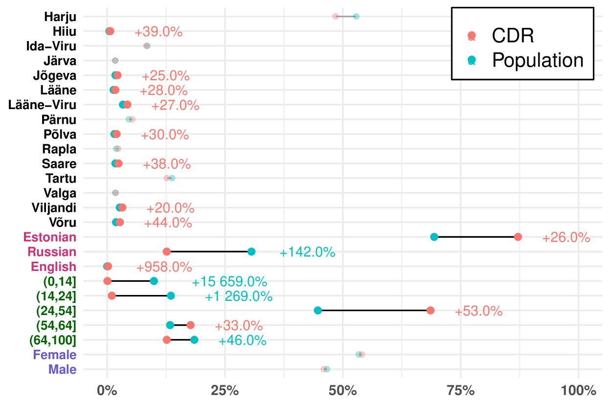
Figure 1: Comparison of actual population of Estonia and users in CDR based on four features. Here, x-axis represents percentage and y-axis represents users’ features from top to bottom namely location (written in black), language (highlighted in purple), age-group (highlighted with green) and gender (highlighted in blue). The sum of all percentages based on each feature is 100 percent for both CDR and actual Estonian population separately. For each feature value, pink dots represent percentage of users in the CDR dataset and seagreen dots represent percentage of people of actual Estonian population. Furthermore, for each feature value, the difference between CDR and actual population percentage is calculated using formula 3. All the differences greater than 20 percent are written and highlighted with text color. For example, for age-group (64,100], difference is +46.0% which means actual population of Estonia is 46 percent more than the representation of users in CDR dataset.

Encoding users’ age. Centered on the official age-group categorization suggested by Europe-Bureau and Statistics Estonia [32], we categorize the age of users into the following five groups: (1) 0-14 years: Children; (2) 15-24 years: Early working age; (3) 25-54 years: Prime working age; (4) 55-64 years: Mature working age; and (5) 65+: Elderly.

In Table II, the Age-Groups row displays the distribution of users in the dataset according to their age-group. E.g., for the age-group (24,54], there exist 83,028 individual users in the dataset that belongs to age-group (24,54].

CDR dataset validation using census dataset. As CDR data contains call records that might not represent the actual interaction among individuals, we need to validate that the CDR data is indeed an acceptable representative of Estonia’s actual population. We compare the distribution of users in the CDR based on four features (location, language, age-group and gender) with the actual Estonian population in Figure 1, where, the x-axis represents percentage and the y-axis represents users’ features. For each feature value (e.g., Harju, Estonian, (24,54], Female, etc.), the percentage of users in CDR and actual population are plotted. Next, the difference between the CDR percentage and actual population percentage is calculated using formula 3 for each feature value.

$$Difference=\frac{|CDR\ \%-Population\ \%|}{min(CDR\ \%,Population\ \%)}*100$$ (3)

The differences greater than 20 percent are written and highlighted with the text color. The features and the difference interpretation from top to bottom on the y-axis are as follows:

1) Location: There are 15 counties in Estonia, with the Harju county, which contains the capital Tallinn being the most populated, followed by the Tartu county as the second most populated, and the Hiiu county as the least populous. From Figure 1, we can observe that the difference between CDR users and the actual population in top-4 populated counties, representing nearly 80 percent of Estonia’s real population, is less than 20 percent[31]. All the counties with a difference of more than 20 percent cover approximately 14 percent of Estonia’s population. Therefore, we can conclude that CDR data is indeed a good representative of the actual Estonian population based on location.

2) Language: As we mentioned earlier that the preferred language of interaction choices in the CDR dataset are either Estonian, Russian, or English. In Figure 1, we can observe that the representation of the Estonian-speaking population is higher in CDR data than the actual Estonian population. On the other hand, this behaviour is reversed for the Russian-speaking population. The possible reason for such behavior is the fact that foreign-language speakers speak mostly with individuals from other countries and prefer to use other cheap mediums to connect, such as Whatsapp, Facebook, Skype, Telegram, etc[33]. Hence, we can conclude that CDR data can be used for calculating segregation based on language.

3) Age-groups: Based on age-group, we observe that mobiles are mostly used by prime working age users (i.e., (24,54]), mature working age users (i.e., (54,64]), and elderly users (i.e., (64,100]). These three age-groups cover approx 99 percent of the CDR dataset and 76 percent of the total Estonian population. Mobile usage percentages for other age-groups are relatively less than their actual population. From this, we can infer that in the CDR dataset, the representation of the prime working age users is significant considering their actual population in Estonia. Thus, we can argue that the prime working age users’ findings can be considered accurate with reasonable confidence. The same is valid for mature working age and elderly users. On the other hand, the representation of children and early working age-group in CDR is less to negligible compared to the actual population, making it difficult to analyze these age-groups.

4) Gender: For both genders (female and male), the difference is less than 20 percent. Thus, we can infer that CDR data is a good gender-based depiction of the real Estonian population.

Based on CDR data validation using Estonian census data, we can infer that the CDR is indeed a fair representative of Estonia’s actual population, and all the study findings on the CDR dataset can be deemed correct with reasonable certainty.

CDR dataset availability. Our dataset is partly location data, and it can not be shared due to privacy concerns. Additionally, despite the fact that the dataset is anonymized at two levels, there is still a small chance that specific persons can be identified. The dataset is owned by our university lab and is accessible for research purposes after signing the NDA.

IV Proposed Methodology

This section first explains the motivation (in Section IV-A) behind proposing new indexes for measuring different aspect of segregation, Individual Segregation Index (ISI), Individual Inclination Index (III), and Overall Behavioural Index (OBI). The OBI is calculated using ISI, and III. The ISI index measures whether segregation exists at individual level (Section IV-B), and III index measures the inclination (Section IV-C).

IV-A Motivation

As mentioned earlier in Section I, the past indexes are over-simplified and use over-reduced information about groups to measure segregation; that is, they use highly aggregated information (the number of individuals in different groups and the ties within and in-between groups), which often results in an imprecise measurement of segregation. Also, many existing indexes (for example, the most well-known dissimilarity index [8]) does not look into the behaviour that results in segregation. In our work, we are using a separate index III to measure the inclination that explains this behaviour by analyzing individuals’ connection preferences.

Moreover, a few indexes measure both segregation and inclination simultaneously (e.g., homophily index [13]. However, the information is over-reduced again, making it impossible to look at the behavior that resulted in the segregation. By behaviour, we mean that how individuals’ of a group are connected to other groups. In this work, we propose the OBI index, which measures the segregation (using ISI and III index), and it is possible to see the individuals’ behaviour of the group of the population that results in the segregation. We can analyze the population’s actual behaviour using OBI index, which is not possible using other existing indexes.

IV-B Individual Segregation Index (ISI)

We first describe annotations that will be used throughout this section. Let $G$ is a set of $n$ number of attribute groups i.e., $G$ = {$g_{1}$, $g_{2}$, $g_{3}$ … $g_{n}$} and $A$ is a set of population distribution for each group {$\alpha_{1}$, $\alpha_{2}$, $\alpha_{3}$ … $\alpha_{n}$}. Then, ISI can be formalised as follows:

$$ISI=\frac{\sum_{i=1}^{n}|P_{g_{i}}-\alpha_{i}|}{2*(1-min(A))}$$ (4)

where, $P_{g_{i}}$ represents the proportion of an individual’s connectivity to group $i$ and $min(A)$ is the minimum value in set $A$.

The ISI index applies to any categorical variable (whether demographic or not), and its range varies between 0 and 1, where 0 means no-segregation (or individuals connectivity follows population distribution) and 1 means high segregation for the population group under investigation. For example, considering Estonia’s three different language speaking population as groups, i.e., Estonian, Russian and English-speaking groups. The population distribution of these groups in Estonia is 0.69, 0.3 and 0.01 [31]. Figure 2 shows the heatmap for ISI index which clearly shows that an individual speaking to only English-speaking individuals is more segregated than an individual connected to only Russian-speaking individuals. Similarly, an individual speaking to only Russian-speaking individuals is more segregated than an individual connected to only Estonian-speaking individuals.

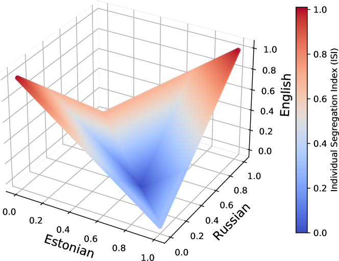
Figure 2: The ISI index heatmap for an individual on different connection combinations to Estonian, Russian and English-speaking population in Estonia.

The ISI index can calculate segregation; however, it fails to detect the segregation behavior’s reasons. Next, we will define the index to identify the connection preference (or inclination) of the segregated individuals.

IV-C Individual Inclination Index (III)

The III index is useful to measure the connection preferences (or inclination) of an individual in a group of the population under investigation. Considering the notations defined in Section IV-B, the III index for an individual that belongs to group $k$ can be defined as follows:

$$III=\begin{cases}\frac{P_{g_{k}}-\alpha_{k}}{P_{g_{k}}}&:P_{g_{k}}-\alpha_{k}\leq 0\\ \frac{P_{g_{k}}-\alpha_{k}}{1-\alpha_{k}}&:P_{g_{k}}-\alpha_{k}\geq 0\end{cases}$$ (5)

where, $P_{g_{k}}$ represents the proportion of an individual’s connectivity to its own group $k$. Please note that for $P_{g_{k}}-\alpha_{k}=0$, both use case are valid.

The III index is applicable to any categorical variable (whether demographic or not), and its range varies between -1 to 1, where -1 means complete inclination towards other groups and 1 means total inclination towards its own group. On the other hand, the value of 0 for III index means no inclination towards any group. Please note that to calculate the III index for an individual, we need to consider its group, which is not a requirement for calculating the ISI index.

IV-D Overall Behavioural Index (OBI)

The OBI index can be used to understand the behaviour of an individual or a group of population. This is calculated using ISI and III index and can be formulated as follows:

$$OBI=\begin{cases}sign(III)*\left(\frac{ISI+abs(III)}{2}\right)&:III\neq 0\\ (-1)*\left(\frac{ISI}{2}\right)&:III=0\end{cases}$$ (6)

where, $sign(III)$ and $abs(III)$ represents the sign and absolute value of the III index respectively. For example, $sign(-0.4)$ will return $-1$ and $abs(-0.4)$ will give $0.4$.

The OBI index considers the behavioural distribution of each individual in the group of the population, and its range varies between -1 to 1, where -1 means highly segregated with a complete inclination towards other groups and 1 also means highly segregated but with a complete inclination towards the same group. The value 0 for OBI index means no segregation. Thus, the OBI index is non-simplified and gives more precise information on whether segregation exists or not. Please note that the average of OBI index for a group can be zero in two possible ways. First, when individuals’ behavioural distribution in a group follows actual population distribution. Second, if OBI index for a group is symmetric about zero as shown in Figure 3, that is OBI and -OBI have the same distribution, and can be written as OBI $\overset{D}{=}$ -OBI.

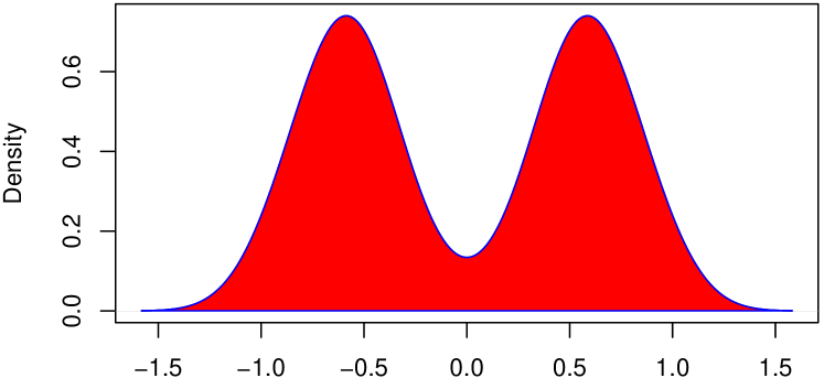
Figure 3: The OBI index distribution for a group. The average of OBI index for the group is zero.

IV-E Example

This section demonstrates how to calculate OBI though a toy example consisting of two groups based on gender, i.e., female and male groups. The connectivity of each individuals is shown in Figure 4. As the population distribution among female and male groups are: 0.6, and 0.4 respectively, therefore, female represents majority group and male minority group.

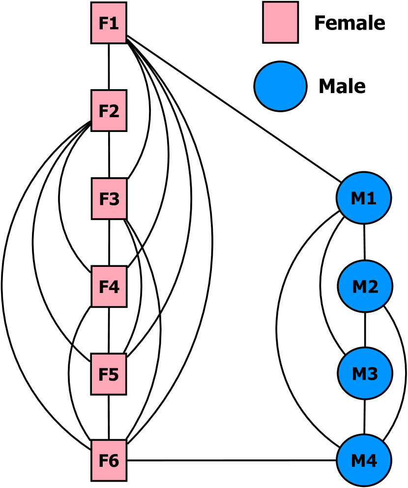
Figure 4: Connectivity network.

	ISI	III	OBI
F1	0.39	0.58	0.48
F2	0.67	1	0.83
F3	0.67	1	0.83
F4	0.67	1	0.83
F5	0.67	1	0.83
F6	0.39	0.58	0.48
M1	0.5	0.58	0.54
M2	1	1	1
M3	1	1	1
M4	0.5	0.58	0.54
Table 3: Index values.

Calculating ISI index. Here, we calculate the ISI index for female $F1$ in Figure 4 that has connectivity to female, and male groups as 5/6 and 1/6 respectively. The ISI index for $F1$ can be calculated as:

$$ISI_{F1}=\frac{|\frac{5}{6}-0.6|+|\frac{1}{6}-0.4|}{2*(1-min(0.6,0.4))}=0.39$$

Table 3 (Column 2) shows ISI index for other females and males which clearly indicates that females ($F2$, $F3$, $F4$ and $F5$) are more segregated than females $F1$ and $F6$. However, males $M2$ and $M3$ are the most segregated individuals in the whole network because males $M2$ and $M3$ are only connected to other males, and male group is a minority group. On the other hand, the females $F2$, $F3$, $F4$ and $F5$ are connected to only other females and are less segregated than males $M2$ and $M3$, because female group is a majority group. Using ISI index, we can identify individuals with high or low segregation; however, to understand their behaviour in-depth, we need to understand their inclination.

Calculating III index. For calculating III index, we need to consider the gender of the individual under investigation. For female $F1$ in Table 3 (Column 3), the III index can be calculated using formula 5 as:

$$III_{F1}=\frac{\frac{5}{6}-0.6}{1-0.6}=0.58$$

Similarly, we can calculate III index for other individuals as well. Here, we can observe that individuals only connected to the same group have the III value as 1.

Calculating OBI index. We can calculate OBI index for female $F1$ in Table 3 (Column 4) using formula 6 as:

$$OBI_{F1}=sign(0.58)*\left(\frac{0.39+abs(0.58)}{2}\right)=0.48$$

Here, we can observe that considering the population distribution in Figure 4, a male only connected to male group is the most segregated, and a female only connected to both female and male group is the least segregated. Figure 5 displays the OBI index distribution for each individual, that highlights the behaviour of each group that results in segregation. The dotted lines represent the average of OBI index for each group.

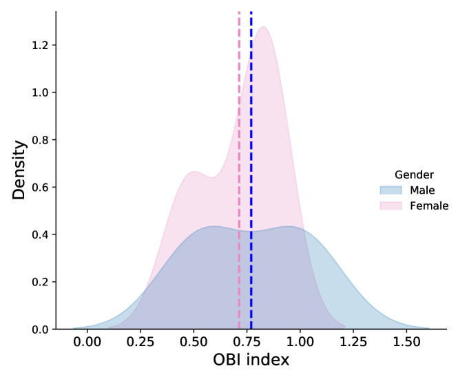
Figure 5: Distribution of OBI index for the Table 3.

V Evaluation

This section starts by briefly describing Freeman’s segregation index (Section V-A) and homophily index (Section V-B), the two commonly used indexes for measuring segregation [34], which are used as baseline to compare with our proposed OBI index. Next, in Section V-C, we measure and compare the OBI with Freeman and homophily index using CDR data.

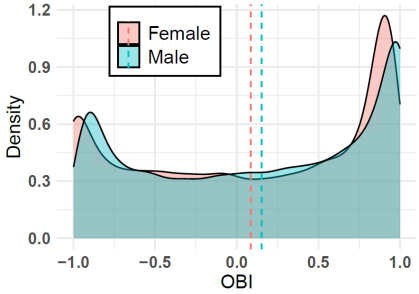
(a)

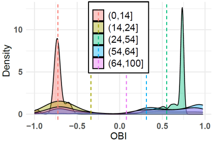
(b)

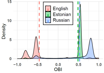
(c)

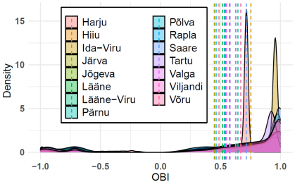
(d)

Figure 6: OBI on (a) gender, (b) age-groups, (c) language, and (d) location (county) features of the CDR dataset.

V-A Freeman’s Segregation Index

The Freeman Segregation Index (FSI) has been extensively used for understanding segregation in the social interaction network [14]. According to FSI, if a given attribute (group label) does not apply to social connection then connections should be randomly distributed with respect to the attribute. Thus, the disparity between cross-group ties expected by chance and observed is used to measure segregation.

Calculating FSI value. Let us consider a network with static attribute groups A and B (of relative size $N_{A}$ and $N_{B}$ with $N_{A}+N_{B}=1$) distributed among nodes uniformly at random and independently of the network structure, such that there is a fraction $P_{AB}=P_{BA}$ of edges between groups, and fractions $P_{AA}$, $P_{BB}$ within each group ($P_{AA}+P_{AB}+P_{BB}=1$). The FSI can be measure using below formula:

$$FSI=1-\frac{X}{E(X)}$$ (7)

where, X is the proportion of between group ties and E(X) is the expected proportion of random ties. The X and E(X) can be calculated using formula 8 and 9 respectively.

$$X=\frac{P_{AB}}{P_{AA}+P_{AB}+P_{BB}}$$ (8)

$$E(X)=\frac{2N_{A}N_{B}}{(N_{A}+N_{B})(N_{A}+N_{B}-1)}$$ (9)

V-B Homophily Index For Measuring The Segregation

Homophily is the tendency of individuals to interact and associate with other individuals. In the past, homophily has been studied in great detail in numerous works [35]. These studies indicate that the similarity is correlated with the connection among individuals and can be categorized based on age, gender, class, ethnicity [36], etc. In this work, we use the Coleman homophily index (HI) [13] for comparison with OBI since HI is commonly used to compares the homophily of groups with different sizes by normalizing the excess homophily of groups by its maximal value [13].

Calculating HI value: Considering the notations defined in Section V-A. In the case of two attribute groups, the probability that a random edge from a node in a group A leads to a node in group A is defined as:

$$T_{AA}=\frac{2P_{AA}}{2P_{AA}+P_{AB}}$$ (10)

Similarly, we can write equation for $T_{BB}$. The HI value for group $A$ ($HI_{A}$) and $B$ ($HI_{B}$) can be calculated using

$$HI_{A}=\frac{T_{AA}-N_{A}}{1-N_{A}}$$ (11)

$$HI_{B}=\frac{T_{BB}-N_{B}}{1-N_{B}}$$ (12)

The range for both $HI_{A}$ and $HI_{B}$ is from -1 to 1, where -1 for $HI_{A}$ means that group $A$ individuals only connects with group $B$ individuals (only in between groups connections), whereas 1 for $HI_{A}$ means that group $A$ individuals only connects with group $A$ individuals (only within-group).

V-C Measuring Segregation Using CDR Dataset

The central goal of segregation indexes is to measure the degree of separation between two or more population groups. When measuring segregation using sampled segregation indexes, one would expect that the relative order of segregation is preserved. For example, in Table II (for feature Languages), the order of segregation according to all segregation indexes (FSI, HI and OBI) is Russian$<$Estonian$<$English, that is, the Russian-speaking population is the most segregated and the English-speaking population is the least segregated. This property of preserving relative order of segregation can be called consistency and formalized as follows:

(Consistency definition). Let the connection network data D be fixed. Any number of segregation indexes $I_{1}$, $I_{2}$, $I_{3}$ … $I_{n}$ are consistent on any features (say X and Y), if the relative order of all indexes are preserved. That is,

$$I_{k}(D,X)>I_{k}(D,Y);\hskip 8.53581pt\forall_{k\in\{1,2,..,n\}}$$ (13)

where, $I_{k}(D,X)$ is the segregation value using segregation index $I_{k}$ on data $D$ and feature $X$.

Consider one more example, in Table II (for feature Age-Groups), age group (64,100] is most segregated according to FSI, on the other hand, both HI and OBI find out that age-group (24,54] is the most segregated. Here, consistency is not reserved. Thus analyzing individual’s behaviour is necessary to report accurate segregation that is possible using OBI.

Figure 6 visualize the individuals’ OBI index distribution based on gender (6(a)), age-group (6(b)), language (6(c)) and location (6(d)). For example, OBI index distribution on Age-Groups shows that children (i.e., (0,14]) and early-working age (i.e., (14,24]) population are more connected to other age groups (see Figure 6(b)). On the other hand, prime-working age (i.e., (24,54]), mature-working age (i.e., (54,64]) and elderly (i.e., (64,100]) are more inclined towards same age group individuals. On comparing the OBI index on Age-Groups with HI index (see Table II), we observe that HI index is not able to measure accurate segregation for children (i.e., (0,14]) and early-working age (i.e., (14,24]) population. Hence, this shows that OBI index can measure segregation more precisely than the other baseline indexes.

VI Discussion and Conclusion

Segregation indexes help in summarizing the relationship between various groups and provide a basis for public policy intervention. But, finding an ideal segregation index from the existing set of indices is challenging for the following reasons. First, due to the complexity of varied dimensions and arrangements in society. Second, due to the over-simplified and over-reduced nature of the past measures. To overcome this, we proposed Overall Behavioural Index (OBI) segregation index which is combination of Individual Segregation Index (ISI) and Individual Inclination Index (III) that reports the segregation as well as the inclination of the population group under investigation. Thus, the OBI index is non-simplified and makes it possible to analyze the connectivity behaviour of individuals of groups that leads to segregation.

We validated the CDR dataset with Estonian census data while interpreting the results and reporting the segregation. To further maintain the data quality, we do not consider the individuals with fewer connections during the analysis. We applied filters at two stages. First, we used the statistical test to identify the significant number of connections, and based on which the individuals with less than six connections are not considered. Second, the individuals with at least six connections with other individuals with known features are considered. A possible limitation of the OBI index is that, it is relatively time-consuming (compared to past indices), as we are avoiding the over-simplification and over-reduction. Thus, reducing the time-complexity of the proposed method is an interesting direction for future research.

References

- [1] R. Farley and W. H. Frey, “Changes in the segregation of whites from blacks during the 1980s: Small steps toward a more integrated society,” American sociological review, pp. 23–45, 1994.
- [2] R. Goel, R. Sharma, and A. Aasa, “Understanding gender segregation through call data records: An estonian case study,” Plos one, vol. 16, no. 3, p. e0248212, 2021.
- [3] J. E. Oliver, “The effects of metropolitan economic segregation on local civic participation,” American journal of political science, 1999.
- [4] M. Meister and A. Niebuhr, “Comparing ethnic segregation across cities—measurement issues matter,” Review of Regional Research, 2020.
- [5] M. Santiago, “A framework for an interdisciplinary understanding of mexican american school segregation,” Multicultural Education Review, vol. 11, no. 2, pp. 69–78, 2019.
- [6] J. B. Ward, S. S. Albrecht, W. R. Robinson, B. W. Pence, J. Maselko, M. N. Haan, and A. E. Aiello, “Neighborhood language isolation and depressive symptoms among elderly us latinos,” Annals of epidemiology, vol. 28, no. 11, pp. 774–782, 2018.
- [7] W. C. Goedel, A. Shapiro, M. Cerdá, J. W. Tsai, S. E. Hadland, and B. D. Marshall, “Association of racial/ethnic segregation with treatment capacity for opioid use disorder in counties in the united states,” JAMA network open, vol. 3, no. 4, pp. e203 711–e203 711, 2020.
- [8] O. D. Duncan and B. Duncan, “A methodological analysis of segregation indexes,” American sociological review, vol. 20, no. 2, 1955.
- [9] D. S. Massey and N. A. Denton, “The dimensions of residential segregation,” Social forces, vol. 67, no. 2, pp. 281–315, 1988.
- [10] C. F. Cortese, R. F. Falk, and J. K. Cohen, “Further considerations on the methodological analysis of segregation indices,” American sociological review, pp. 630–637, 1976.
- [11] D. W. Wong, “Spatial indices of segregation,” Urban studies, 1993.
- [12] O. D. Duncan and B. Duncan, “Residential distribution and occupational stratification,” American journal of sociology, vol. 60, no. 5, 1955.
- [13] J. Coleman, “Relational analysis: The study of social organizations with survey methods,” Human organization, vol. 17, no. 4, pp. 28–36, 1958.
- [14] L. C. Freeman, “Segregation in social networks,” Sociological Methods & Research, vol. 6, no. 4, pp. 411–429, 1978.
- [15] B. S. Morgan, “The segregation of socio-economic groups in urban areas: a comparative analysis,” Urban Studies, vol. 12, no. 1, 1975.
- [16] S. Lieberson, “An asymmetrical approach to segregation.” Ethnic segregation in cities., pp. 61–82, 1981.
- [17] P. A. Jargowsky, “Take the money and run: Economic segregation in us metropolitan areas,” American sociological review, pp. 984–998, 1996.
- [18] M. Poulsen, R. Johnston, and J. Forrest, “Intraurban ethnic enclaves: introducing a knowledge-based classification method,” Environment and planning A, vol. 33, no. 11, pp. 2071–2082, 2001.
- [19] L. A. Brown and S.-Y. Chung, “Spatial segregation, segregation indices and the geographical perspective,” Population, space and place, 2006.
- [20] M. J. White, “The measurement of spatial segregation,” American journal of sociology, vol. 88, no. 5, pp. 1008–1018, 1983.
- [21] R. Grannis, “Discussion: Segregation indices and their functional inputs,” Sociological methodology, vol. 32, no. 1, pp. 69–84, 2002.
- [22] R. Morrill, “On the measure of geographic segregation,” in Geography research forum, vol. 11, 1991, pp. 25–36.
- [23] S. F. Reardon and D. O’Sullivan, “Measures of spatial segregation,” Sociological methodology, vol. 34, no. 1, pp. 121–162, 2004.
- [24] A. Horn, “Measuring multi-ethnic spatial segregation in south african cities,” South African Geographical Journal, vol. 87, no. 1, 2005.
- [25] D. W. Wong, “Formulating a general spatial segregation measure,” The Professional Geographer, vol. 57, no. 2, pp. 285–294, 2005.
- [26] F. F. Feitosa, G. Camara, A. M. V. Monteiro, T. Koschitzki, and M. P. Silva, “Global and local spatial indices of urban segregation,” International Journal of Geographical Information Science, 2007.
- [27] R. G. Cromley and D. M. Hanink, “Focal location quotients: specification and applications,” Geographical analysis, vol. 44, 2012.
- [28] L. Anselin, “Local indicators of spatial association—lisa,” Geographical analysis, vol. 27, no. 2, pp. 93–115, 1995.
- [29] A. Getis and J. K. Ord, “The analysis of spatial association by use of distance statistics,” in Perspectives on spatial data analysis. Springer, 2010, pp. 127–145.
- [30] D. W. Wong, “Measuring multiethnic spatial segregation,” Urban Geography, vol. 19, no. 1, pp. 77–87, 1998.
- [31] S. Estonia, “Statistical database,” Population data, vol. 2012, 2012. [Online]. Available: https://www.stat.ee/population
- [32] ——, “Mean annual population by sex and age group.” [Online]. Available: https://www.stat.ee/esms-metadata?code=30205
- [33] S. Taipale and M. Farinosi, “The big meaning of small messages: The use of whatsapp in intergenerational family communication,” in International Conference on Human Aspects of IT for the Aged Population. Springer, 2018, pp. 532–546.
- [34] A. Mele, “Does school desegregation promote diverse interactions? an equilibrium model of segregation within schools,” American Economic Journal: Economic Policy, vol. 12, no. 2, pp. 228–57, 2020.
- [35] A. Asikainen, G. Iñiguez, J. Ureña-Carrión, K. Kaski, and M. Kivelä, “Cumulative effects of triadic closure and homophily in social networks,” Science Advances, vol. 6, no. 19, p. eaax7310, 2020.
- [36] A. Sahasranaman and H. J. Jensen, “Ethnicity and wealth: The dynamics of dual segregation,” PloS one, vol. 13, no. 10, p. e0204307, 2018.