Distributed Banach-Picard Iteration: Application to Distributed EM and Distributed PCA

Distributed Banach-Picard Iteration: Application to Distributed Parameter Estimation and PCA

Abstract

In recent work, we proposed a distributed Banach-Picard iteration (DBPI) that allows a set of agents, linked by a communication network, to find a fixed point of a locally contractive (LC) map that is the average of individual maps held by said agents. In this work, we build upon the DBPI and its local linear convergence (LLC) guarantees to make several contributions. We show that Sanger’s algorithm for principal component analysis (PCA) corresponds to the iteration of an LC map that can be written as the average of local maps, each map known to each agent holding a subset of the data. Similarly, we show that a variant of the expectation-maximization (EM) algorithm for parameter estimation from noisy and faulty measurements in a sensor network can be written as the iteration of an LC map that is the average of local maps, each available at just one node. Consequently, via the DBPI, we derive two distributed algorithms – distributed EM and distributed PCA – whose LLC guarantees follow from those that we proved for the DBPI. The verification of the LC condition for EM is challenging, as the underlying operator depends on random samples, thus the LC condition is of probabilistic nature.

I Introduction

Parameter estimation from noisy data and dimensionality reduction are two of the most fundamental tasks in signal processing and data analysis. In many scenarios, such as sensor networks and IoT, the underlying data is distributed among a collection of agents that cooperate to jointly solve the problem, i.e., find a consensus solution without sharing the data or sending it to a central unit [1]. This paper addresses the two problems above mentioned in a distributed setting, proposing and analysing two algorithms that are instances of the distributed Banach-Picard iteration (DBPI), which we have recently introduced and proved to enjoy local linear convergence [2]. In this introductory section, after presenting the formulations and motivations of the two problems considered, we review the DBPI and summarize our contributions and the tools that are used for the convergence proofs.

I-A Problem Statement: Dimensionality Reduction

Dimensionality reduction aims at representing high-dimensional data in a lower dimensional space, which can be crucial to reduce the computational complexity of manipulating and processing this data, and is a core task in modern data analysis, machine learning, and related areas. The standard linear dimensionality reduction tool is principal component analysis (PCA), which allows expressing a high-dimensional dataset on the basis formed by the top eigenvectors of its sample covariance matrix. PCA first appeared in the statistics community in the beginning of the 20th century [3] and became one of the workhorses of statistical data analysis, with dimensionality reduction being a notable application. Nowadays, with the ever increasing collection of data by spatially dispersed agents, developing algorithms for distributed PCA constitutes a relevant area of research – see, e.g., [4, 5, 6, 7, 8, 9, 10, 11, 12] (master-slave communication architecture), and [13, 14, 15, 16, 17, 18, 19, 20] (arbitrarily meshed network communication architecture). For a recent and comprehensive review on these works, see, e.g., [21]; for a very recent work see [22].

In the (arbitrarily meshed network) distributed setting, consider a set of $N$ agents linked by an undirected and connected communication graph; the nodes are the agents, and the edges represent the communication channels between the agents. Each agent $n$ holds a finite set of points in $\mathbb{R}^{d}$, $\mathbf{Y}_{n}\subseteq\mathbb{R}^{d}$, and the agents seek to collectively find the top $m$ eigenvectors of

$$C=\frac{1}{M}\sum_{n=1}^{N}C_{n},$$

(assumed to be positive definite, i.e., $C\succ 0$), where $M=\sum_{n=1}^{N}|\mathbf{Y}_{n}|$, i.e., the sum of the cardinalities of each $\mathbf{Y}_{n}$, and

$$C_{n}=\sum_{y\in\mathbf{Y}_{n}}yy^{T}.$$

I-B Problem Statement: Distributed Parameter Estimation with Noisy and Faulty Measurements

Consider a collection of spatially distributed sensors monitoring the environment, a common scenario for information processing or decision making tasks see, e.g., [23, 24, 25, 26, 27, 28, 29, 30]. Often, these sensors communicate wirelessly, maybe in a harsh environment, which may result in faulty communications or sensor malfunctions [31]. The setup is modelled as follows: $N$ agents, linked by an undirected and connected communication graph, each holding an independent observation given by

$$Y_{n}=Z_{n}h_{n}^{T}\mu^{\star}+W_{n},\quad n=1,\ldots,N.$$ (1)

In (1), $\mu^{\star}\in\mathbb{R}^{d}$ is a fixed and unknown parameter, each $h_{n}\in\mathbb{R}^{d}$ is assumed to be known only at agent $n$, $\{W_{j}\}_{n=1}^{N}$ are independent and identically distributed (i.i.d.) zero-mean Gaussian random variables with variance $(\sigma^{\star})^{2}$, and $\{Z_{n}\}_{n=1}^{N}$ are i.i.d. Bernoulli random variables ($Z_{n}\in\{0,1\}$) with $f_{Z_{n}}(z_{n}|p^{\star})=(p^{\star})^{z_{n}}(1-p^{\star})^{1-z_{n}}$. This formulation models a scenario where sensor $n$ measures the parameter $\mu^{\star}$ with probability $p^{\star}$ and, with probability $1-p^{\star}$, it senses only noise, indicating a transducer failure [31]. The agents seek to collectively estimate $\mu^{\star}$, treating $p^{\star}$ and $\sigma^{\star}$ as nuisance (or latent) parameters. Observe that if the binary variables $Z_{n}$ were not random, but fixed and known, the model could be regarded as a (distributed) linear regression problem. However, the randomness introduces an extra layer of difficulty accounting for potential sensor failures.

A decentralized algorithm, rather than one where each sensor sends its data to a central node, is potentially more robust to faulty wireless communications that may render a sensor useless. Moreover, a decentralized algorithm can yield considerable energy savings [23], a very desirable feature.

I-C Distributed Banach-Picard Iteration (DBPI)

Our recent work [2] addressed a general distributed setup where $N$ agents, linked by a communication network, collaborate to collectively find an attractor $x^{\star}$ of a map $H$ that can be implicitly represented as an average of local maps, i.e.,

$$H=\frac{1}{N}\sum_{n=1}^{N}H_{n},$$

where $H_{n}$ is the map held by agent $n$. As defined in [2], an attractor $x^{\star}$ of $H$ is a fixed point thereof, $H(x^{\star})=x^{\star}$, satisfying

$$\rho\big{(}\mathbf{J}_{H}(x^{\star})\big{)}<1,$$ (2)

where $\rho\big{(}\mathbf{J}_{H}(x^{\star})\big{)}$ is the spectral radius of the Jacobian of $H$ at $x^{\star}$. Moreover, the map $H$ is not assumed to have a symmetric Jacobian and no global structural assumptions (e.g., Lipschitzianity or coercivity) are made.

The main contributions of [2] are a distributed algorithm to find $x^{\star}$ – DBPI – and the proof that it enjoys the local linear convergence of its centralized counterpart, i.e., of the (standard) Banach-Picard iteration: $x^{k+1}=H(x^{k})$.

I-D Contributions and Related Work

In this work, we propose addressing the distributed inference problems described in Subsections I-A and I-B using two instantiations of DBPI. More concretely, we propose:

1. A distributed algorithm for PCA, which results from considering a map that can be implicitly written as an average of local maps and that has as a fixed point the solution to the PCA problem.

2. An algorithm that stems from formulating the problem described in Subsection I-B as a fixed point of a map induced by the stationary equations of the corresponding maximum likelihood estimation (MLE) criterion. This map corresponds to the iterations of a slightly modified EM algorithm for a mixture of linear regressions [32].

The guarantees of local linear convergence for these distributed algorithms involve verifying condition (2) for the maps inducing them, which allows invoking the results from [2]. Consequently, a great portion of this paper is devoted to proving that (2) holds for these maps, which is far from trivial.

The distributed PCA problem (see [23] for a review of distributed PCA) described in Subsection I-A was addressed in [33] , where an algorithm termed accelerated distributed Sanger’s algorithm (ADSA) was proposed. The authors consider a “mini-batch variant” of Sanger’s algorithm (SA, see [34]) and, inspired by [35], arrive at ADSA. Although no proof of convergence was presented in [33], very recent work by the same authors proves convergence of their algorithm [36]. Our contributions in this context are twofold: we show that ADSA is recovered by applying DBPI to SA, and that condition (2) holds for SA, thus, the guarantees of local convergence follow directly as a consequence of the results in [2]. We mention that no computer simulations of ADSA are presented in this work, since these can be found in [33].

The problem presented in Subsection I-B was addressed in [31], where (1) is regarded as a finite mixture model [37]. To estimate $\mu^{\star}$, the authors proposed a distributed version of the expectation-maximization (EM [38]) algorithm, termed diffusion-averaging distributed EM (DA-DEM). However, DA-DEM, very much in the spirit of [39, 40], uses a diminishing step-size to achieve convergence, leading to a sublinear convergence rate. Our contribution is an algorithm for this problem that extends a slightly modified version of the centralized EM algorithm to distributed settings. The key challenge is to show that we can “expect” condition (2) to hold, and we dedicate a considerable amount of effort to this endeavor. We use the term “expect”, since the operator underlying DBPI depends on the observed samples and, therefore, the existence of an attractor is a probabilistic question. Finally, we compare our algorithm with DA-DEM through Monte Carlo simulations, confirming the linear convergence rate of our algorithm and the sublinear convergence of DA-DEM.

There is considerable work on the “probabilistic linear convergence” of EM [41], [42], [43]. However, neither the results in [41], nor those in [42] encompass the mixture model underlying (1). The mixture of regressions presented in [43] bears some similarity with the model underlying (1), but it is not the same: in [43], $p$ is fixed at $1/2$ and $Z_{n}\in\{-1,1\}$ (rather than $\{0,1\}$), thus there are no measurements that are just noise. Furthermore, [43] is primarily concerned with statistical guarantees for the error with respect to the ground truth, while we address the goal of establishing (2).

As mentioned in [31], there are two other relevant works on distributed EM, namely, [44] and [45]. However (see [31]), both these works address a different problem of Gaussian mixture density estimation. Moreover, in the case of [44], the algorithm demands a cyclic network topology, and, in [45] the algorithm requires higher computational load on each node, since it is based on alternating direction method of multipliers.

To summarize, we show that ADSA [33] is an instance of DBPI and propose an algorithm to solve the mixture model underlying (1), also as an instance of DBPI. Consequently, their corresponding guarantees of local linear convergence result from the attractor condition (2) for the map underlying the corresponding centralized counterparts. We compare DA-DEM and our proposed algorithm through numerical Monte Carlo simulations, and the results confirm the linear convergence of our algorithm and the sublinear convergence of DA-DEM.

I-E Organization of the Paper

Section II briefly reviews the DBPI proposed in [2] and the main convergence result therein proved. The characterization of the fixed points of the “mini-batch” variant of Sanger’s algorithm, as well as the attractor condition, are presented in Section III. Section IV describes the centralized variant of EM underlying the proposed distributed algorithm for the problem in Subsection I-B, presents the verification of the attractor condition, and reports the results of simulations comparing DBPI with DA-DEM.

I-F Notation

The set of real $n$ dimensional vectors with positive components is denoted by $\mathbb{R}^{n}_{>0}$. Matrices and vectors are denoted by upper and lower case letters, respectively. The spectral radius of a matrix $A$ is denoted by $\rho(A)$ and its Frobenius norm by $\|A\|_{F}$. Given a map $H$, $\mathbf{J}_{H}(x)$, and $dH(x)$ denote, respectively, the Jacobian of $H$ at $x$ and the differential of $H$ at $x$. Given a vector $v$, $v_{s}$ denotes its $s$th component; given a matrix $A$, $A_{st}$ denotes the element on the $s$th row and $t$th column and $A^{T}$ its transpose. The $d$-dimensional identity matrix is denoted by $I_{d}$, $\mathbf{1}_{d}$ is the $d$-dimensional vector of ones, and $\mathbf{0}_{m,n}$ is the $m\times n$ matrix of zeros. Whenever convenient, we will denote a vector with two stacked blocks, $[v^{T},u^{T}]^{T}$, simply as $(v,u)$. Given a square matrix $A$, $\mathcal{U}(A)$ is an upper triangular matrix of the same dimension as $A$ and whose upper triangular part coincides with that of $A$. Given a norm $\|\cdot\|$, $\bar{B}^{\|\cdot\|}_{\delta,\theta}$ denotes the closed ball of center $\theta$ and radius $\delta$ with respect to $\|\cdot\|$. Random variables and vectors are denoted by upper case letters and, for random variable $Y$, the probability density (or mass) function of $Y$ is denoted by $f_{Y}$. The probability density of a Gaussian of mean $\mu$ and variance $\sigma^{2}$ is denoted by $\mathcal{N}(\cdot|\mu,\sigma^{2})$.

II Review of Distributed Banach-Picard Iteration

Consider a network of $N$ agents, where the interconnection structure is represented by an undirected connected graph: the nodes correspond to the agents and an edge between two agents indicates they can communicate (are neighbours). In the scenario considered in [2], each agent $n\in\{1,...,N\}$ holds an operator $H_{n}:\mathbb{R}^{d}\to\mathbb{R}^{d}$, and the goal is to compute a fixed point of the average operator

$$H=\frac{1}{N}\sum_{n=1}^{N}H_{n}.$$ (3)

Each agent $n$ is restricted to performing computations involving $H_{n}$ and communicating with its neighbours.

Our only assumption about $H$ is the existence of a locally attractive fixed point $x^{\star}$, i.e., satisfying (2).

Let $R$ be the map on $\mathbb{R}^{dN}$ defined, for $z=[z_{1}^{T},\ldots,z_{N}^{T}]^{T}$ (with $z_{j}\in\mathbb{R}^{d}$ held by agent $j$) by

$$R(z)=\Big{[}\big{(}H_{1}(z_{1})-z_{1}\big{)}^{T},\ldots,\big{(}H_{N}(z_{N})-z_{N}\big{)}^{T}\Big{]}^{T},$$ (4)

and let $W=\tilde{W}\otimes I_{d}$, where $\tilde{W}$ is the so-called Metropolis weight matrix associated to the communication graph [46]. The algorithm proposed in [2] is presented in Algorithm 1, where $\alpha\in\mathbb{R}_{>0}$.

Algorithm 1 Distributed Banach-Picard Iteration (DBPI)

1:  Initialization:

$$z^{0} \in\mathbb{R}^{dN},$$

$$z^{1} =Wz^{0}+\alpha R(z^{0}),$$

2:  Update:

$$z^{k+2}=(I+W)z^{k+1}-\frac{I+W}{2}z^{k}+\alpha\big{(}R(z^{k+1})-R(z^{k})\big{)}.$$

Informally, in [2], we show that $\alpha$ can be chosen such that if $z^{k}$ gets sufficiently close to $\mathbf{1}\otimes x^{\star}$, then it converges to $\mathbf{1}\otimes x^{\star}$ at least linearly (the precise statement and proof can be found in [2]). Notice that $z$ being equal to $\mathbf{1}\otimes x^{\star}$ means that all agents are in consensus, holding a copy of the fixed point $x^{\star}$.

III Distributed PCA

III-A Algorithm

We obtain a distributed algorithm for solving the PCA problem described in section I-A as an instantiation of DBPI by introducing a map $H$ with a fixed point at the desired solution. Moreover, the guarantees of local linear convergence follow as a result of verifying (2).

The “mini batch variant” of Sanger’s algorithm (SA) proposed in [33] and inspired by [34] is the Banach-Picard iteration

$$X^{k+1}=H(X^{k}),$$

where $H:\mathbb{R}^{d\times m}\to\mathbb{R}^{d\times m}$ is given by

$$H(X)=X+\eta\Big{(}CX-X\mathcal{U}\big{(}X^{T}CX\big{)}\Big{)},$$ (5)

and $\mathcal{U}$ was defined in Subsection I-F. Observe that $H$ can be written as an average of local maps, i.e.,

$$H=\frac{1}{N}\sum_{n=1}^{N}H_{n},$$

where $H_{n}:\mathbb{R}^{d\times m}\to\mathbb{R}^{d\times m}$ is defined by

$$H_{n}(X)=X+\eta\Big{(}\frac{N}{M}C_{n}X-X\mathcal{U}\big{(}X^{T}\frac{N}{M}C_{n}X\big{)}\Big{)}.$$ (6)

Let $R$ be the map on $\mathbb{R}^{(d\times m)N}$ defined, for $z=[z_{1}^{T},\ldots,z_{N}^{T}]^{T}$, as in (4), with $H_{n}$ as in (6). The distributed algorithm presented in [33], named ADSA, is exactly the DBPI, i.e., Algorithm 1, with this choice of $R$.

III-B Convergence: Main Results

The convergence analysis amounts to verifying the attractor condition (2) for $H$, thus establishing, as a corollary of the results in [2], the local linear convergence of Algorithm 1 with each $H_{n}$ in (4) defined as in (6) (equivalently, ADSA).

We start with the following lemma (proved in Appendix D) showing that the solution sought in the PCA problem is a fixed point of $H$ (as defined in (5)).

Lemma 1.

Let $C\succ 0$. If $X^{\star}\in\mathbb{R}^{d\times m}$ satisfies

$$CX^{\star}=X^{\star}\mathcal{U}((X^{\star})^{T}CX^{\star})$$ (7)

then, each column of $X^{\star}$ is either $0$ or a unit-norm eigenvector of $C$. Moreover, the columns are orthogonal, i.e., $(X^{\star})^{T}X^{\star}$ is diagonal with the diagonal elements being either one or zero.

The following theorem guarantees that the Banach-Picard iteration of $H$ has local linear convergence to its fixed points.

Theorem 1.

Let $\lambda_{1}>\ldots>\lambda_{m}>\lambda_{m+1}\geq\ldots\geq\lambda_{d}>0$ be the eigenvalues of $C$. Suppose that $X^{\star}$ is a $d\times m$ matrix such $Cx^{\star}_{i}=\lambda_{i}x^{\star}_{i}$ (where $x_{i}^{\star}$ denotes the $i$th column of $X^{\star}$ and $C$ is as defined in (5)), for $i=1,\ldots,m$, and $(X^{\star})^{T}X^{\star}=I_{m}$. Then, there exists $\eta^{\star}$ such that, for $0<\eta<\eta^{\star}$,

$$\rho\big{(}\mathbf{J}_{H}(X^{\star})\big{)}<1.$$

Remark 1.

The invertibility of $C$ that is assumed in the statements of Lemma 1 and Theorem 1 is not a big restriction. In fact, if $C\succeq 0$ rather than $C\succ 0$, then $\tilde{C}=C+\epsilon I$ satisfies $\tilde{C}\succ 0$ and has the same eigenvectors as $C$.

III-C Proof of Theorem 1

First, note that $H(X)=I+\eta S(X)$, where

$$S(X)=CX-\mathcal{U}\big{(}X^{T}CX\big{)}.$$

This implies $\mathbf{J}_{H}(X^{\star})=I+\eta\mathbf{J}_{S}(X^{\star})$, and, as a consequence, each eigenvalue of $\mathbf{J}_{H}(X^{\star})$ is of the form $1+\eta\beta$, with $\beta$ being an eigenvalue of $\mathbf{J}_{S}(X^{\star})$. The idea is to show that these eigenvalues $\beta$ of $\mathbf{J}_{S}(X^{\star})$ enjoy a key property: they are real-valued and negative, $\beta<0$. Such property means that, for sufficiently small $\eta>0$, we have $|1+\eta\beta|<1$. To establish this key property, we divide the proof of Theorem 1 in two lemmas: Lemma 2 and Lemma 3.

Lemma 2 will show that the eigenvalues of $\mathbf{J}_{S}(X^{\star})$ coincide with those of the linear map from $\mathbb{R}^{d\times m}$ to $\mathbb{R}^{d\times m}$ given by

$$W\to\hat{D}W-WD-A\mathcal{U}(DA^{T}W+W^{T}AD),$$ (8)

where

$$D=\mbox{diag}(\lambda_{1},\ldots,\lambda_{m}),$$ (9)

$$\hat{D}=(\lambda_{1},\ldots,\lambda_{m},\lambda_{m+1},\ldots,\lambda_{d}),$$ (10)

and

$$A=\begin{bmatrix}I_{m}\\ \mathbf{0}_{d-m,m}\end{bmatrix}.$$ (11)

Lemma 3 will show that the eigenvalues of (8) are real and negative.

Lemma 2.

Let $X^{\star}$ satisfy the conditions of Theorem 1. The eigenvalues of $\mathbf{J}_{S}(X^{\star})$, where

$$S:\mathbb{R}^{d\times m} \to\mathbb{R}^{d\times m}$$

$$X \to CX-\mathcal{U}(X^{T}CX)$$

coincide with those of the linear map given by

$$W\to\hat{D}W-WD-A\mathcal{U}(DA^{T}W+W^{T}AD),$$

with $D$, $\hat{D}$, and $A$ given by, respectively, (9), (10), and (11).

Proof.

From the rules of matrix differential calculus (see [47] and [48]), the differential of $S$ at $X$, denoted by $dS(X)$, is the linear map

$$dX\to CdX-(dX)\mathcal{U}(X^{T}CX)-Xd\big{(}\mathcal{U}(X^{T}CX)\big{)}(X).$$ (12)

Observe that $\mathcal{U}$ is a linear map, thus the composition rule for differentials further yields

$$d\big{(}\mathcal{U}(X^{T}CX)\big{)}(X)=\mathcal{U}\big{(}(dX)^{T}CX+X^{T}CdX\big{)}.$$ (13)

By assumption, $CX^{\star}=X^{\star}D$ with $D$ given by (9), thus combining this with (12) and (13), $dS(X^{\star})$, which we denote by $\hat{S}$ to simplify the notation, is given by

$$\hat{S}(dX) =CdX-(dX)D$$

$$\;\;\;\;-X^{\star}\mathcal{U}\big{(}(dX)^{T}X^{\star}D+D(X^{\star})^{T}dX\big{)}.$$

The eigenvalues of $\mathbf{J}_{S}(X^{\star})$ coincide with those of $dS(X^{\star})=\hat{S}$, under the identification between Jacobians and differentials (see [47]); hence, we will study the eigenvalues of the latter.

Let $\hat{X}^{\star}$ be an extension of $X^{\star}$ to an orthonormal basis of eigenvectors of $C$, i.e., $(\hat{X}^{\star})^{T}\hat{X}^{\star}=I_{d}$ and $C\hat{X}^{\star}=\hat{X}^{\star}\hat{D}$, where $\hat{D}$ is given by (10). To understand the eigenvalues of $\hat{S}$, consider the linear map given by

$$V(dX)\to\hat{X}^{\star}dX$$ (14)

and observe that $V$ is an invertible linear map (in fact $V^{-1}(dX)=(\hat{X}^{\star})^{T}dX$). Eigenvalues are invariant under a similarity transformation, hence, the eigenvalues of $\hat{S}$ coincide with those of $V^{-1}\circ\hat{S}\circ V$ which, after renaming $dX$ by $W$, just amounts to the linear map

$$W\to\hat{D}W-WD-A\mathcal{U}(DA^{T}W+W^{T}AD),$$

with $D$, $\hat{D}$, and $A$ given by, respectively, (9), (10), and (11). ∎

In the proof of the following lemma it is crucial that the eigenvalues are in decreasing order.

Lemma 3.

Let $D$, $\hat{D}$, and $A$ be defined, respectively, by (9), (10), and (11). The eigenvalues of the linear map from $\mathbb{R}^{d\times m}$ to $\mathbb{R}^{d\times m}$ defined by

$$W\to\hat{D}W-WD-A\mathcal{U}(DA^{T}W+W^{T}AD)$$ (15)

are real and negative.

Proof.

Let $Z$ be an eigenvector (note that $Z$ is in fact a matrix) of (15) associated to the eigenvalue $\beta$, i.e.,

$$\hat{D}Z-ZD-A\mathcal{U}(DA^{T}Z+Z^{T}AD)=\beta Z;$$ (16)

next, we show that $\beta<0$.

Consider a block partition of $Z$ of the form

$$Z=\begin{bmatrix}\tilde{Z}\\ \bar{Z}\end{bmatrix},$$

where $\tilde{Z}$ and $\bar{Z}$ are, respectively, $m\times m$ and $(d-m)\!\times\!m$ matrices. The eigenvalue matrix equation (16) induces the following system of matrix equations

$$D\tilde{Z}-\tilde{Z}D-\mathcal{U}(D\tilde{Z}+\tilde{Z}^{T}D) =\beta\tilde{Z},$$ (17)

$$\bar{D}\bar{Z}-\bar{Z}D =\beta\bar{Z},$$ (18)

where $\bar{D}=\mbox{diag}(\lambda_{m+1},\ldots,\lambda_{d})$.

There are two non-mutually-exclusive cases to consider: $\tilde{Z}\neq 0$ or $\bar{Z}\neq 0$ ($Z\neq 0$, by virtue of being an eigenvector).

Case 1

Suppose that $\bar{Z}_{st}\neq 0$. Then, (18) implies that

$$\lambda_{m+s}\bar{Z}_{st}-\lambda_{t}\bar{Z}_{st}=\beta\bar{Z}_{st},$$

and, hence, $\beta=\lambda_{m+s}-\lambda_{t}<0$.

Case 2

Suppose that $\tilde{Z}_{st}\neq 0$. This case splits in two: either $s>t$ or $s\leq t$. If $s>t$, then (17) and the “upper triangularization” operation yields

$$\lambda_{s}\tilde{Z}_{st}-\lambda_{t}\tilde{Z}_{st}=\beta\tilde{Z}_{st},$$ (19)

which, after dividing by $\tilde{Z}_{st}$, yields $\lambda_{s}-\lambda_{t}=\beta<0$. If $s\leq t$, then,

$$\beta\tilde{Z}_{st} =\lambda_{s}\tilde{Z}_{st}-\lambda_{t}\tilde{Z}_{st}-\mathcal{U}(D\tilde{Z}+\tilde{Z}^{T}D)_{st}$$

$$=\lambda_{s}\tilde{Z}_{st}-\lambda_{t}\tilde{Z}_{st}-\lambda_{s}\tilde{Z}_{st}-\lambda_{t}\tilde{Z}_{ts}$$

$$=-\lambda_{t}(\tilde{Z}_{st}+\tilde{Z}_{ts}).$$

Next, notice that if $s<t$, then $\tilde{Z}_{ts}$ can be assumed to be $0$, since, otherwise, we could deal with it as in (19) with the roles of $s$ and $t$ reversed to conclude $\beta<0$. Hence, assuming $\tilde{Z}_{ts}=0$, we obtain, after division by $\tilde{Z}_{st}$, that $\beta=-\lambda_{t}<0.$ Finally, if $s=t$, then $\beta=-2\lambda_{t}<0.$ ∎

IV Parameter estimation with noisy measurements

IV-A Roadmap

This is a rather long section, hence the need for a road map. The analysis of (1) is simplified if the measurements are identically distributed besides being just independent and, therefore, we start by introducing a probability distribution on the vectors $h_{n}$ and a joint model on $(Y,H)$.

To estimate $\mu^{\star}$ ($p^{\star}$ and $\sigma^{\star}$ are treated as nuisance parameters), we consider the stationary equations imposed by equating to zero the gradient of the log-likelihood function, a necessary condition satisfied by the maximum likelihood estimator (MLE). Once the particular form of the stationary equations is realized, we reformulate them as a fixed point equation of the form $g_{1}\circ g_{2}(\theta^{\star})=\theta^{\star}$ that naturally suggests the Banach-Picard iteration

$$\theta^{k+1}=g_{1}\circ g_{2}(\theta^{k}).$$

Observing that the map $g_{1}\circ g_{2}$ cannot be written as an average of local maps, we switch to the map $H=g_{2}\circ g_{1}$, which can be implicitly written as an average of local maps. With this map, we arrive at a distributed algorithm by considering the map $R$ (see section II) arising from $H$ and appealing to Algorithm 1.

Finally, we observe that the existence of a fixed point of $H=g_{2}\circ g_{1}$ satisfying (2) follows from the existence of a fixed point of $g_{1}\circ g_{2}$ satisfying (2). The final part of the section is thus devoted to verifying (2) for the map $g_{1}\circ g_{2}$, and to a numerical simulation comparing Algorithm 1 and DA-DEM from [31].

IV-B Identically distributed observations

Let $\theta^{\star}=(\mu^{\star},p^{\star},(\sigma^{\star})^{2})\in\Theta=\mathbb{R}^{d}\times(0,1)\times(0,+\infty)$ be an unknown and fixed vector which we term the ground truth.

The agents’ measurements are assumed to be independent (see (1)); however, they are not identically distributed, given the presence of the vectors $h_{n}$ in (1). To address this issue, let $Z\in\{0,1\}$, $H\in\mathbb{R}^{d}$, and $Y\in\mathbb{R}$ be, respectively, a binary random variable, a random vector, and a real random variable. Suppose the joint density on $(Y,H,Z)$ factors as

$$f_{Y,H,Z}\big{(}y,h,z|\theta^{\star}\big{)}=f_{H}(h)f_{Z}(z|p^{\star})f_{Y|H,Z}\big{(}y|h,z,\mu^{\star},(\sigma^{\star})^{2}\big{)},$$ (20)

where

$$f_{H}(h) =\mathcal{N}(h|0,I_{d}),$$

$$f_{Z}(z|p^{\star}) =(p^{\star})^{z}(1-p^{\star})^{1-z},$$

and

$$f_{Y|H,Z}\big{(}y|h,z,\theta^{\star}\big{)}=\mathcal{N}\big{(}y|h^{T}\mu^{\star},(\sigma^{\star})^{2}\big{)}^{z}\mathcal{N}\big{(}y|0,(\sigma^{\star})^{2}\big{)}^{1-z}.$$ (21)

Instead of assuming that the $h_{n}$ are fixed as in [31], we assume that each sensor $n$ has a measurement $(y_{n},h_{n})$, where $(y_{n},h_{n},z_{n})$ was drawn from (20), but agent $n$ has no knowledge of $z_{n}$. After marginalization, the joint density of $Y,H$ is given by

$$f_{Y,H}\big{(}y,h|\theta^{\star})=f_{H}(h)f_{Y|H}(y|h,\theta^{\star})$$ (22)

$$= f_{H}(h)\Big{(}p^{\star}\mathcal{N}\big{(}y|h^{T}\mu^{\star},(\sigma^{\star})^{2}\big{)}+(1-p^{\star})\mathcal{N}\big{(}y|0,(\sigma^{\star})^{2}\big{)}\Big{)},$$

which is a mixture model [49].

To estimate $\mu^{\star}$, the agents seek $\theta\in\Theta$ such that

$$\frac{1}{N}\sum_{n=1}^{N}\nabla_{\theta}\phi(y_{n},h_{n},\theta)=0,$$ (23)

where $\phi$ is the log-likelihood of $(Y,H)$, i.e.,

$$\phi(y,h,\theta) =\log(f_{Y,H}(y,h|\theta)$$ (24)

$$=\log\big{(}f_{H}(h)\big{)}+\log\big{(}f_{Y|H}(y|h,\theta)\big{)}.$$

Since $f_{H}(h)$ does not depend on $\theta$,

$$\nabla_{\theta}\phi(y,h,\theta)=\nabla_{\theta}\log\big{(}f_{Y|H}(y|h,\theta)\big{)};$$

in other words, (23) is a necessary condition satisfied by the MLE corresponding to the log-likelihood function $\log f_{Y|H}(y|h,\theta)$, thus independent of $f_{H}$.

IV-C Gradient of $\phi$ and the centralized algorithm

Before explicitly writing the stationary equations corresponding to (23), we introduce the responsibility functions [49],

$$r(y,h,\theta)=\frac{p\mathcal{N}(y|h^{T}\mu,\sigma^{2})}{p\mathcal{N}(y|h^{T}\mu,\sigma^{2})+(1-p)\mathcal{N}(y|0,\sigma^{2})}.$$ (25)

Notice that $r(y,h,\theta)=\mathbb{P}(z=1|y,h,\theta)$, the posterior probability that the observation $y$ was not a result of measuring only noise.

For reasons that will be clear later, the following set of equalities, which can be easily verified, will be convenient:

$$\sigma^{2}\nabla_{\mu}\phi(y,h,\theta) =r(y,h,\theta)(y-h^{T}\mu)h$$ (26)

$$p+p(1-p)\frac{\partial\phi}{\partial p}(y,h,\theta) =r(y,h,\theta)$$

$$\sigma^{2}+2(\sigma^{2})^{2}\frac{\partial\phi}{\partial\sigma^{2}}(y,h,\theta) =r(y,h,\theta)(y-h^{T}\mu)^{2}$$

$$+\big{(}1-r(y,h,\theta)\big{)}y^{2}.$$

Using (26), (23) can be explicitly written as

$$\Big{(}\frac{1}{N}\sum_{n=1}^{N}\Gamma(y_{n},h_{n},\theta)\Big{)}\mu =\frac{1}{N}\sum_{n=1}^{N}\psi(y_{n},h_{n},\theta)$$ (27)

$$p =\frac{1}{N}\sum_{n=1}^{N}r(y_{n},h_{n},\theta)$$ (28)

$$\sigma^{2} =\frac{1}{N}\sum_{n=1}^{N}\gamma(y_{n},h_{n},\theta),$$ (29)

where

$$\Gamma(y,h,\theta) =r(y,h,\theta)hh^{T},$$

$$\psi(y,h,\theta) =r(y,h,\theta)yh,$$

$$\gamma(y,h,\theta) =r(y,h,\theta)(y-h^{T}\mu)^{2}+\big{(}1-r(y,h,\theta)\big{)}y^{2}.$$

If the matrix $\frac{1}{N}\sum_{n=1}^{N}\Gamma(y_{n},h_{n},\theta)$ is invertible, then (27)-(29) can be written as a fixed point equation. This constitutes the motivation for the centralized algorithm that we suggest next (see Algorithm 2) and from which we will derive the distributed version; observe that it is the Banach-Picard iteration motivated by (27)-(29).

Another way to write (30)-(32) (see Algorithm 2 below) is $\theta^{k+1}=g_{1}\circ g_{2}(\theta^{k})$, where

$$g_{2}(\theta)=\frac{1}{N}\Big{(} \sum_{n=1}^{N}\Gamma(y_{n},h_{n},\theta),\sum_{n=1}^{N}\psi(y_{n},h_{n},\theta),$$

$$\sum_{n=1}^{N}r(y_{n},h_{n},\theta),\sum_{n=1}^{N}\gamma(y_{n},h_{n},\theta)\Big{)}$$

and

$$g_{1}(\Gamma,\psi,p,\sigma^{2})= \big{(}\Gamma^{-1}\psi,p,\sigma^{2}\big{)}.$$

Algorithm 2 Centralized variant of EM

  Initialization:

$$\theta^{0}=\big{(}\mu^{0},p^{0},(\sigma^{0})^{2}\big{)}\in\Theta$$

  Update: $\theta^{k+1}=\big{(}\mu^{k+1},p^{k+1},(\sigma^{k+1})^{2}\big{)}$, where

$$\mu^{k+1} =\Big{(}\frac{1}{N}\sum_{n=1}^{N}\Gamma(y_{n},h_{n},\theta^{k})\Big{)}^{-1}\frac{1}{N}\sum_{n=1}^{N}\psi(y_{n},h_{n},\theta^{k})$$ (30)

$$p^{k+1} =\frac{1}{N}\sum_{n=1}^{N}r(y_{n},h_{n},\theta^{k})$$ (31)

$$(\sigma^{k+1})^{2} =\frac{1}{N}\sum_{n=1}^{N}\gamma(y_{n},h_{n},\theta^{k}).$$ (32)

IV-D Distributed Algorithm

Although, $g_{2}$ is an average of local maps, the map $g_{1}\circ g_{2}$ is not, due to the matrix inversion in (30). As a consequence, (30)-(32) cannot be directly extended to a distributed algorithm. However, switching the order of $g_{1}$ and $g_{2}$ results in a map that can be implicitly written as an average of local maps. In fact, instead of the iteration $\theta^{k+1}=g_{1}\circ g_{2}(\theta^{k})$, consider the iteration

$$z^{k+1}=H(z^{k}),$$

where $H=g_{2}\circ g_{1}$ and $z=(\Gamma,\psi,p,\sigma^{2})$.

Let

$$G_{n}(\theta)=\Big{(} \Gamma\big{(}y_{n},h_{n},\theta\big{)},\psi\big{(}y_{n},h_{n},\theta\big{)},$$

$$r\big{(}y_{n},h_{n},\theta\big{)},\gamma\big{(}y_{n},h_{n},\theta\big{)}\Big{)},$$

and it follows that $H=\frac{1}{N}\sum_{n=1}^{N}H_{n}$, where

$$H_{n}(z)=G_{n}\circ g_{1}(z).$$ (33)

To conclude, the distributed algorithm we suggest amounts to Algorithm 1, with $R:\mathbb{R}^{(d^{2}+d+2)N}\to\mathbb{R}^{(d^{2}+d+2)N}$ defined, for $z=(z_{1}^{T},\ldots,z_{N}^{T})^{T}$, as in (4), and $H_{n}$ as in (33). Additionally, following [31], we suggest the initialization

$$z_{n}^{0}=\sum_{m=1}^{N}\tilde{W}_{nm}G_{m}\big{(}\frac{y_{n}h_{n}}{h_{n}^{T}h_{n}},\frac{1}{2},\frac{y_{n}^{2}}{2}\big{)}.$$ (34)

Some remarks are due:

a)

The existence of a fixed point of $g_{1}\circ g_{2}$ satisfying (2) is addressed in section IV-E;

b)

The existence of a fixed point of $g_{2}\circ g_{1}$ satisfying (2) follows from the existence of a fixed point of $g_{1}\circ g_{2}$ satisfying (2), by the chain rule;

c)

Expanding (32) yields

$$(\sigma^{k+1})^{2} =\frac{1}{N}\sum_{n=1}^{N}r(y_{n},h_{n},\theta^{k})(y_{n}-h_{n}^{T}\mu^{k})^{2}$$

$$+\big{(}1-r(y_{n},h_{n},\theta^{k})\big{)}y_{n}^{2},$$

and, if the update rule is modified according to

$$(\sigma^{k+1})^{2} =\frac{1}{N}\sum_{n=1}^{N}r(y_{n},h_{n},\theta^{k})(y_{n}-h_{n}^{T}\mu^{k+1})^{2}$$

$$+\big{(}1-r(y_{n},h_{n},\theta^{k})\big{)}y_{n}^{2},$$

then, a straightforward manipulation recovers the EM algorithm presented in [31]. Moreover, the EM algorithm derived in [31] is still amenable to a distributed implementation using Algorithm 1. However, we found it easier to prove (2) for this variant of EM, than for the standard EM.

IV-E Convergence Analysis

The proof of local linear convergence of the centralized variant of EM, i.e., Algorithm 2, is not trivial. In fact, this question is probabilistic in nature, because updates (30)-(32) depend on observations that are, in turn, samples from a probability distribution. Before presenting the main convergence result (Theorem 3), we need to introduce some definitions and only one mild assumption that is instrumental in the proof of Lemma 4 below: the Fisher information at $\theta^{\star}$, given by,

$$\mbox{I}(\theta^{\star})=\mathbb{E}_{\theta^{\star}}\Big{[}\nabla_{\theta}\phi(y,h,\theta^{\star})\big{(}\nabla_{\theta}\phi(y,h,\theta^{\star})\big{)}^{T}\Big{]},$$ (35)

is non-singular.

Let $T_{N}=g_{1}\circ g_{2}$ denote the map underlying the Banach-Picard iteration (30)-(32). A straightforward manipulation, using (26), shows that

$$T_{N}(\theta)=\theta+\big{(}A_{N}(\theta)\big{)}^{-1}\frac{1}{N}\sum_{n=1}^{N}\nabla_{\theta}\phi(y_{n},h_{n},\theta),$$

where

$$A_{N}(\theta)=\begin{bmatrix}\frac{1}{N}\sum_{n=1}^{N}\frac{1}{\sigma^{2}}\Gamma(y_{n},h_{n},\theta)&\mathbf{0}&\mathbf{0}\\ \mathbf{0}&\frac{1}{p(1-p)}&0\\ \mathbf{0}&0&\frac{1}{2(\sigma^{2})^{2}}\end{bmatrix}.$$

Before stating the main result, we introduce the “infinite sample” map, i.e.,

$$T(\theta)=\theta+\big{(}A(\theta)\big{)}^{-1}\mathcal{L}(\theta),$$

where

$$A(\theta)=\begin{bmatrix}\mathbb{E}_{\theta^{\star}}\Big{[}\frac{1}{\sigma^{2}}\Gamma(y,h,\theta)\Big{]}&\mathbf{0}&\mathbf{0}\\ \mathbf{0}&\frac{1}{p(1-p)}&0\\ \mathbf{0}&0&\frac{1}{2(\sigma^{2})^{2}}\end{bmatrix},$$

and

$$\mathcal{L}(\theta)=\mathbb{E}_{\theta^{\star}}\big{[}\nabla\phi(y,h,\theta)\big{]}.$$

The next lemma shows that $T$ is a “natural” map to consider.

Lemma 4.

The “infinite sample map”, i.e., $T$, has the following properties

a)

For fixed $\theta$, $T_{N}(\theta)$ converges in probability to $T(\theta)$;

b)

The ground truth $\theta^{\star}$ is a fixed point of $T$, i.e. $T(\theta^{\star})=\theta^{\star}$;

c)

The attractor condition (2) holds for $T$ at $\theta^{\star}$, i.e.,

$$\rho\big{(}\mathbf{J}_{T}(\theta^{\star})\big{)}<1.$$

Proof.

The proof of b) amounts to a straightforward verification and the proof of a) follows by the weak law of large numbers, hence, we will focus on the proof of c) which relies on the principle of missing information (see [50], page 101), and the assumption on the Fisher Information condition, i.e., (35).

Under suitable regularity conditions (see appendix A) that hold for the model (LABEL:JointOnYandH),

$$\mathbb{E}_{\theta^{\star}}\Big{[}\nabla^{2}_{\theta}\phi(y,h,\theta^{\star})\Big{]}=-\mbox{I}(\theta^{\star}).$$

Additionally, a simple calculation reveals that $A(\theta^{\star})$ coincides with the Fisher information of the complete data model (20), i.e.,

$$A(\theta^{\star})=\mbox{I}_{c}(\theta^{\star}).$$

The non-singularity assumption on $\mbox{I}(\theta^{\star})$ (see (35)), together with the principle of missing information (see [50], page 101), implies that

$$0\prec\mbox{I}(\theta^{\star})\preceq\mbox{I}_{c}(\theta^{\star}).$$

All these observations show that

$$\mathbf{J}_{T}(\theta^{\star})=I-\big{(}\mbox{I}_{c}(\theta^{\star})\big{)}^{-1}\mbox{I}(\theta^{\star}),$$ (36)

and, Theorem 7.7.3 of [51], together with $0\prec\mbox{I}(\theta^{\star})\preceq\mbox{I}_{c}(\theta^{\star})$, implies that

$$\rho\big{(}\mathbf{J}_{T}(\theta^{\star})\big{)}<1,$$

concluding that $\theta^{\star}$ is an attractor of $T$. ∎

We recall that the goal of this section is to show that the probability that $T_{N}$ has an attractor approaches $1$ as $N$ tends to infinity; the strategy is to derive this from the existence of an attractor of $T$, i.e., c) in Lemma 4. Pointwise convergence in probability, i.e., a) in Lemma 4, is not enough to arrive at this result. In fact, the proof is built on a stronger notion that is a probabilistic version of uniform, rather than pointwise, convergence of maps. This is the content of Theorem 2 below.

Observe that if $\theta_{N}$ is a fixed point of $T_{N}$, then

$$\mathbf{J}_{T_{N}}(\theta_{N})=I+\big{(}A_{N}(\theta_{N})\big{)}^{-1}\frac{1}{N}\sum_{n=1}^{N}\nabla_{\theta}^{2}\phi(y_{n},h_{n},\theta_{N}),$$

so let

$$T_{N}^{\prime}(\theta) =I+\big{(}A_{N}(\theta)\big{)}^{-1}\frac{1}{N}\sum_{n=1}^{N}\nabla_{\theta}^{2}\phi(y_{n},h_{n},\theta),$$

$$T^{\prime}(\theta) =I+\big{(}A(\theta)\big{)}^{-1}\mathbb{E}_{\theta^{\star}}\Big{[}\nabla^{2}_{\theta}\phi(y,h,\theta)\Big{]}.$$

Remark 2.

Note that the maps $T_{N}^{\prime}(\theta)$ and $T^{\prime}(\theta)$ only coincide with the jacobian maps $\mathbf{J}_{T_{N}}(\theta)$ and $\mathbf{J}_{T}(\theta)$ at fixed points.

The uniform convergence in probability is expressed in the next theorem, whose proof can be found in appendix C. For the statement, recall (see the notation section) that $\bar{B}^{\|\cdot\|}_{\delta,\theta^{\star}}$ is the closed ball of center $\theta^{\star}$ and radius $\delta$, with respect to the metric induced by the norm $\|\cdot\|$.

Theorem 2.

Let $\delta>0$ and $\|\cdot\|$ be any norm. With $T_{N}$, $T_{N}^{\prime}$, $T^{\prime}$, and $T$ as defined above,

$$\sup_{\theta\in\bar{B}^{\|\cdot\|}_{\delta,\theta^{\star}}}\big{\|}T_{N}(\theta)-T(\theta)\big{\|}\to 0$$ (37)

$$\sup_{\theta\in\bar{B}^{\|\cdot\|}_{\delta,\theta^{\star}}}\big{\|}T_{N}^{\prime}(\theta)-T^{\prime}(\theta)\big{\|}\to 0$$ (38)

both in probability, as $N\to\infty$.

We now state the main convergence result.

Theorem 3.

There exists $\delta>0$ and a norm $\|\cdot\|$ such that

$$\mathbb{P}_{\theta^{\star}}\Big{(}\sup_{\theta\in\bar{B}^{\|\cdot\|}_{\delta,\theta^{\star}}}\big{\|}T_{N}(\theta)-\theta^{\star}\|\leq\delta\Big{)} \to 1\quad\text{and}$$

$$\mathbb{P}_{\theta^{\star}}\Big{(}\sup_{\theta\in\bar{B}^{\|\cdot\|}_{\delta,\theta^{\star}}}\big{\|}T_{N}^{\prime}(\theta)\|<1\Big{)} \to 1,$$

where $\|T_{N}^{\prime}(\theta)\|$ is the induced matrix norm.

Before presenting the proof, we explain why Theorem 3 encapsulates the notion that, with probability approaching $1$, the map $T_{N}$ has an attractor. Let

$$\mathcal{A}_{N} =\big{\{}(\mathbf{y},\mathbf{h})\in\mathbb{R}^{N}\times\mathbb{R}^{dN}:\sup_{\theta\in\bar{B}^{\|\cdot\|}_{\delta,\theta^{\star}}}\big{\|}T_{N}(\theta)-\theta^{\star}\|\leq\delta\big{\}}$$

$$\mathcal{B}_{N} =\big{\{}(\mathbf{y},\mathbf{h})\in\mathbb{R}^{N}\times\mathbb{R}^{dN}:\sup_{\theta\in\bar{B}^{\|\cdot\|}_{\delta,\theta^{\star}}}\big{\|}T_{N}^{\prime}(\theta)\|<1\big{\}}.$$

Remark 3.

Informally, observe that the set $\mathcal{A}_{N}$ is the set of “samples” where the ball $\bar{B}_{\delta,\theta^{\star}}^{\|\cdot\|}$ is invariant under $T_{N}$, i.e,

$$T_{N}\big{(}\bar{B}_{\delta,\theta^{\star}}^{\|\cdot\|}\big{)}\subseteq\bar{B}_{\delta,\theta^{\star}}^{\|\cdot\|},$$

and that the set $\mathcal{B}_{N}$ is, from remark 2, the set of “samples” where the Jacobian of $T_{N}$ satisfies (2) at a fixed points. By noting that a continuous map from a convex compact space into itself has a fixed point (Brouwer’s fixed point theorem), it follows that if $(\mathbf{y},\mathbf{h})$ is in $\mathcal{A}_{N}$, then $T_{N}$ has a fixed point. Moreover, if $(\mathbf{y},\mathbf{h})$ is in $\mathcal{A}_{N}\cap\mathcal{B}_{N}$ then $T_{N}$ has a fixed point satisfying (2). All of this is made precise below.

The statement of Theorem 3 is that the (non-random sequences) $\mathbb{P}_{\theta^{\star}}(\mathcal{A}_{N})$ and $\mathbb{P}_{\theta^{\star}}(\mathcal{B}_{N})$ both tend to $1$. The inequalities

$$\mathbb{P}_{\theta^{\star}}(\mathcal{A}_{N})+\mathbb{P}_{\theta^{\star}}(\mathcal{B}_{N})-1 \leq\mathbb{P}_{\theta^{\star}}(\mathcal{A}_{N}\cap\mathcal{B}_{N})\leq\mathbb{P}_{\theta^{\star}}(\mathcal{A}_{N})$$

imply that

$$\mathbb{P}_{\theta^{\star}}(\mathcal{A}_{N}\cap\mathcal{B}_{N})\to 1.$$

Now note that, if both inequalities hold, namely

$$\sup_{\theta\in\bar{B}^{\|\cdot\|}_{\delta,\theta^{\star}}}\big{\|}T_{N}(\theta)-\theta^{\star}\|\leq\delta$$ (39)

$$\sup_{\theta\in\bar{B}^{\|\cdot\|}_{\delta,\theta^{\star}}}\big{\|}T_{N}^{\prime}(\theta)\|<1,$$ (40)

then (39), together with Brouwer’s fixed point theorem (see [53], page 180) implies that $T_{N}$ has a fixed point $\theta_{N}$ in $\bar{B}^{\|\cdot\|}_{\delta,\theta^{\star}}$ (this idea is loosely inspired by [54], page 69). Moreover, being a fixed point, at a $\theta_{N}$ it holds (see remark 2) that $T^{\prime}_{N}(\theta_{N})=\mathbf{J}_{T_{N}}(\theta_{N})$, so, (40) implies that

$$\rho\big{(}\mathbf{J}_{T_{N}}(\theta_{N})\big{)}\leq\big{\|}\mathbf{J}_{T_{N}}(\theta_{N})\|\leq\sup_{\theta\in\bar{B}^{\|\cdot\|}_{\delta,\theta^{\star}}}\big{\|}T_{N}^{\prime}(\theta)\|<1.$$

This explains why Theorem 3 expresses the notion that we can “expect” (2) to hold for $T_{N}$. In fact, from the above, the event

$$\mathcal{C}_{N}=\big{\{}(\mathbf{y},\mathbf{h}):T_{N}\text{ has a fixed point satisfying \eqref{JacobianCondition}}\big{\}}\\$$

contains the event $\mathcal{A}_{N}\cap\mathcal{B}_{N}$, and the probability of this last event is approaching 1.

Proof of Theorem 3

Let $\|\cdot\|$ be any norm. Then

$$\|T_{N}(\theta)-\theta^{\star}\|\leq\|T_{N}(\theta)-T(\theta)\|+\|T(\theta)-\theta^{\star}\|.$$ (41)

From Lemma 4 c),

$$\rho\big{(}\mathbf{J}_{T}(\theta^{\star})\big{)}<1.$$

From the proof of Ostrowski’s Theorem (see [55], page 300), there exists a norm $\|\cdot\|$ on $\mathbb{R}^{d+2}$, an open neighborhood $\mathcal{V}$ of $\theta^{\star}$, and $\lambda<1$, such that

1)

$\|T(\theta)-\theta^{\star}\|\leq\lambda\|\theta-\theta^{\star}\|$, for $\theta\in\mathcal{V}$;

2)

$\|\mathbf{J}_{T}(\theta^{\star})\|<1$, where here the norm is the induced matrix norm.

Choose $\delta$ sufficiently small such that

i)

$\bar{B}^{\|\cdot\|}_{\delta,\theta^{\star}}\subseteq\mathcal{V}$;

ii)

$\|T^{\prime}(\theta)\|=\|\mathbf{J}_{T}(\theta)\|\leq\beta<1$, for $\theta\in\bar{B}^{\|\cdot\|}_{\delta,\theta^{\star}}$,

where the validity of ii) follows from the compactness of $\bar{B}^{\|\cdot\|}_{\delta,\theta^{\star}}$ and the continuity of $T^{\prime}$.

Now, for any $\theta\in\bar{B}^{\|\cdot\|}_{\delta,\theta^{\star}}$, (41) implies that

$$\|T_{N}(\theta)-\theta^{\star}\|\leq\|T_{N}(\theta)-T(\theta)\|+\lambda\delta$$

and, hence,

$$\sup_{\theta\in\bar{B}^{\|\cdot\|}_{\delta,\theta^{\star}}}\big{\|}T_{N}(\theta)-\theta^{\star}\big{\|}\leq\sup_{\theta\in\bar{B}^{\|\cdot\|}_{\delta,\theta^{\star}}}\big{\|}T_{N}(\theta)-T(\theta)\big{\|}+\lambda\delta.$$ (42)

A similar reasoning shows that

$$\sup_{\theta\in\bar{B}^{\|\cdot\|}_{\delta,\theta^{\star}}}\big{\|}T_{N}^{\prime}(\theta)\|\leq\sup_{\theta\in\bar{B}^{\|\cdot\|}_{\delta,\theta^{\star}}}\big{\|}T_{N}^{\prime}(\theta)-T^{\prime}(\theta)\big{\|}+\beta.$$ (43)

To conclude, we appeal to Theorem 2, and we show that it implies the result. Let $\epsilon_{1}=(1-\lambda)\delta$ and $\epsilon_{2}=\frac{1-\beta}{2}$. From the properties of $\lambda$ and $\beta$, it holds that $\epsilon_{1}>0$ and $0<\epsilon_{2}<1$. By the definition of convergence in probability, it holds that

$$\mathbb{P}_{\theta^{\star}}\Big{(}\sup_{\theta\in\bar{B}^{\|\cdot\|}_{\delta,\theta^{\star}}}\big{\|}T_{N}(\theta)-T(\theta)\|\leq\epsilon_{1}\Big{)}\to 1$$

$$\mathbb{P}_{\theta^{\star}}\Big{(}\sup_{\theta\in\bar{B}^{\|\cdot\|}_{\delta,\theta^{\star}}}\big{\|}T_{N}^{\prime}(\theta)-T^{\prime}(\theta)\|\leq\epsilon_{2}\Big{)}\to 1.$$

From (42), (43), and the forms of $\epsilon_{1}$ and $\epsilon_{2}$, we conclude the result.

IV-F Simulations

In this section, we compare our algorithm with the one from [31] (DA-DEM) through Monte Carlo simulations. The parameters generated once and fixed throughout all Monte Carlo runs were: $d=3$, $N=100$, a unit-norm vector $\mu^{\star}\in\mathbb{R}^{d}$, $p^{\star}=0.7$, and an undirected connected graph on $N$ nodes with connectivity radius $r_{c}=0.18$ .

Each Monte Carlo run consisted in

1)

Generating a data set: each $h_{n}$ was independently sampled from a Gaussian with zero mean and covariance $I_{3}$; the variance of the noise $(\sigma^{\star})^{2}$ was generated according to

$$(\sigma^{\star})^{2}=\frac{\|\mathbf{H}\|_{F}^{2}}{N\times\mbox{SNR}},$$

with $\mathbf{H}^{T}=[h_{1}\ldots h_{N}]$ and where SNR is the signal to noise ratio (we experimented with $\text{SNR}\in\{10\text{dB},20\text{dB}\}$). Finally, each $y_{n}$ was sampled according to $f_{Y|H}$ (see (LABEL:JointOnYandH)), with $h_{n}$, $\mu^{\star}$, $p^{\star}$, and $(\sigma^{\star})^{2}$.

2)

Computing $10000$ iterations of the algorithm proposed in [31], with $\rho\in\{2,3,4\}$, and of Algorithm 1, with $\alpha\in\{0.001,0.005,0.01\}$. Both algorithms were initialized according to (34).

The performance metrics consisted in finding a fixed point using the centralized operators as follows.

We first computed

$$\theta^{0}(\alpha)=\frac{1}{N}\sum_{n=1}^{N}g_{1}\big{(}z_{n}^{10000}(\alpha)\big{)}$$ (44)

$$\theta^{0}(\rho)=\frac{1}{N}\sum_{n=1}^{N}\hat{g}_{1}\big{(}z_{n}^{10000}(\rho)\big{)},$$ (45)

where: $\alpha\in\{0.001,0.005,0.01\}$; $\rho\in\{2,3,4\}$; $\hat{g}_{1}$ corresponds to the map arising from the standard EM algorithm derived in [31]. In fact, as seen in [31], the EM algorithm can be written as

$$\theta^{k+1}=\hat{g}_{1}\circ\hat{g_{2}}(\theta^{k}),$$

where

$$\hat{g}_{2}(\theta)=\frac{1}{N}\Big{(} \sum_{n=1}^{N}\Gamma(y_{n},h_{n},\theta),\sum_{n=1}^{N}\psi(y_{n},h_{n},\theta),$$

$$\sum_{n=1}^{N}r(y_{n},h_{n},\theta),\sum_{n=1}^{N}y_{n}^{2}\Big{)}$$

and

$$\hat{g}_{1}(\Gamma,\psi,p,a)= \big{(}\Gamma^{-1}\psi,p,a-\psi^{T}\Gamma^{-1}\psi\big{)}.$$

We ran the algorithms, with initialization as in (44) and (45), given by

$$\theta^{k+1}(\alpha)=g_{1}\circ g_{2}\big{(}\theta^{k}(\alpha)\big{)}$$

$$\theta^{k+1}(\rho)=\hat{g}_{1}\circ\hat{g}_{2}\big{(}\theta^{k}(\rho)\big{)},$$

until we found $\theta^{\star}(\alpha)$ and $\theta^{\star}(\rho)$ satisfying

$$\Big{\|}\theta^{\star}(\alpha)-g_{1}\circ g_{2}\big{(}\theta^{\star}(\alpha)\big{)}\Big{\|}\leq 10^{-10}$$

$$\Big{\|}\theta^{\star}(\rho)-\hat{g}_{1}\circ\hat{g}_{2}\big{(}\theta^{\star}(\rho)\big{)}\Big{\|}\leq 10^{-10}.$$

The error at iteration $k$ of the distributed algorithms was then computed as

$$\frac{1}{N}\sum_{n=1}^{N}\Big{\|}\pi_{1}\circ g_{1}\big{(}(z_{n}^{k}(\alpha)\big{)}-\theta^{\star}(\alpha)\Big{\|}$$

$$\frac{1}{N}\sum_{n=1}^{N}\Big{\|}\pi_{1}\circ\hat{g}_{1}\big{(}(z_{n}^{k}(\rho)\big{)}-\theta^{\star}(\rho)\Big{\|},$$

where $\pi_{1}$ is the projection onto the average, i.e., $\pi_{1}(\mu,p,\sigma^{2})=\mu$ (as mentioned before, $p$ and $\sigma^{2}$ were treated as nuisance parameters).

The number of Monte Carlo tests was $100$ and the errors at iteration $k$ were averaged out of $100$ for each $\alpha$ and $\rho$. The results for two different SNR values are shown in logarithmic scale in Figures 1 and 2.

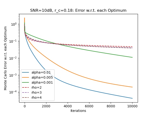
Figure 1: The figure shows the result of the Monte Carlo simulation of the error with respect to each optimum for an $\text{SNR}=10$dB and a connectivity radius of $0.18$. The dashed curves correspond to the algorithm from [31] with parameter $\rho\in\{2,3,4\}$ and the non-dashed curves correspond to the DBPI algorithm with parameter $\alpha\in\{0.001,0.005,0.01\}$.

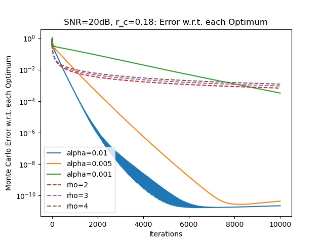
Figure 2: The figure shows the result of the Monte Carlo simulation of the error with respect to each optimum for an $\text{SNR}=20$dB and a connectivity radius of $0.18$. The dashed curves correspond to the algorithm from [31] with parameter $\rho\in\{2,3,4\}$ and the non-dashed curves correspond to the DBPI algorithm with parameter $\alpha\in\{0.001,0.005,0.01\}$.

The simulations show, as expected from the theory, that Algorithm 1 converges linearly and clearly outperforms the algorithm from [31], which, given its diminishing step-size, is bound to converge only sub-linearly. Moreover, both algorithms require just one round of communications per iteration.

V Conclusion

This article builds upon the distributed Banach-Picard algorithm and its convergence properties provided in [2] to make two main contributions: we provided a proof of local linear convergence for the distributed PCA algorithm suggested in [33], thereby filling a gap left by that work; starting from the distributed Banach-Picard iteration, we proposed a distributed algorithm for solving the parameter estimation problem from noisy and faulty measurements that had been addressed in [31]. Unlike the algorithm in [31], which uses diminishing step sizes, thus exhibiting sublinear convergence rate, the proposed instance of the distributed Banach-Picard iteration is guaranteed to have local linear convergence. Numerical experiments confirm the theoretical advantage of the proposed method with respect to that from [31].

Appendix A Regularity Conditions

Theorem 4.

Let $K\subset\Theta$ be a compact set containing $\theta^{\star}$. Then, for all $\theta\in K$,

$$\Big{|}\frac{\partial^{i}\phi}{\partial^{i_{1}}x_{1}\ldots\partial^{i_{k}}x_{k}}(y,h,\theta)\Big{|}\leq\mathcal{P}^{\phi}_{\partial^{i_{1}}x_{1}\ldots\partial^{i_{k}}x_{k}}(|y|,|h_{1}|,\ldots,|h_{d}|)$$ (46)

$$\Big{|}\frac{\partial^{i}r}{\partial^{i_{1}}x_{1}\ldots\partial^{i_{k}}x_{k}}(y,h,\theta)\Big{|}\leq\mathcal{P}^{r}_{\partial^{i_{1}}x_{1}\ldots\partial^{i_{k}}x_{k}}(|y|,|h_{1}|,\ldots,|h_{d}|),$$ (47)

where $\sum_{j=1}^{K}i_{j}=i\geq 1$, $x_{1},\ldots,x_{k}$ are dummy variables in $\{\mu_{1},\ldots,\mu_{d},p,\sigma^{2}\}$ (i.e. consider partial diferentiation with respect to the components of $\theta$), and where

$$\mathcal{P}^{r}_{\partial^{i_{1}}x_{1}\ldots\partial^{i_{k}}x_{k}}\quad\text{and}\quad\mathcal{P}^{\phi}_{\partial^{i_{1}}x_{1}\ldots\partial^{i_{k}}x_{k}}$$

are polynomials.

We start with a proof of (47). Note that $r$ satisfies the following differential equations

$$\frac{\partial r}{\partial\mu_{i}}(y,h,\theta) =\big{(}1-r(\theta)\big{)}r(\theta)\frac{y-h^{T}\mu}{\sigma^{2}}\mu_{i},\quad i=1,\ldots,d,$$

$$\frac{\partial r}{\partial p}(y,h,\theta) =\frac{1}{p(1-p)}r(\theta)\big{(}1-r(\theta)\big{)},$$

$$\frac{\partial r}{\partial\sigma^{2}}(y,h,\theta) =\Big{(}\frac{(y-h^{T}\mu)^{2}}{2(\sigma^{2})^{2}}-\frac{y^{2}}{2(\sigma^{2})^{2}}\Big{)}r(\theta)\big{(}1-r(\theta)\big{)}.$$

We deduce that

$$\frac{\partial r}{\partial\lambda}(y,h,\theta)=\frac{\tilde{\mathcal{P}}_{\lambda}^{r}(r(\theta),y,h,\theta)}{\tilde{\mathcal{Q}}_{\lambda}^{r}(p,\sigma^{2})},$$ (48)

where $\tilde{\mathcal{P}}_{\lambda}^{r}$ and $\tilde{\mathcal{Q}}_{\lambda}^{r}$ are polynomials and $\lambda$ is a dummy variable in $\{\mu_{1},\ldots,\mu_{d},p,\sigma^{2}\}$.

The chain rule of differentiation, the quotient rule of differentiation and the form (48) imply that

$$\frac{\partial^{i}r}{\partial^{i_{1}}x_{1}\ldots\partial^{i_{k}}x_{k}}(y,h,\theta)=\frac{\tilde{\mathcal{P}}_{\partial^{i_{1}}x_{1}\ldots\partial^{i_{k}}x_{k}}^{r}(r(\theta),y,h,\theta)}{\tilde{\mathcal{Q}}_{\partial^{i_{1}}x_{1}\ldots\partial^{i_{k}}x_{k}}^{r}(p,\sigma^{2})}.$$ (49)

The result now follows easily from $0<r(\theta)\leq 1$, the compactness of $K$ and the identity (49).

The inequality (46) follows from (49) and the form of the gradient of $\phi$ in (26). This concludes the proof of Theorem 4.

An immediate corollary of Theorem 4 is that the absolute values of the partial derivatives of both $\phi$ and $r$ are dominated by functions whose expectation exists and is finite; this is the content of the following result.

Theorem 5.

Let $\mathcal{P}$ be a polynomial in $d+1$ variables. Then

$$\mathbb{E}_{\theta^{\star}}\big{[}\mathcal{P}(|y|,|h_{1}|,\ldots,|h_{d}|)\big{]}$$

exists and is finite.

To prove this theorem, observe that $\mathcal{P}(|y|,|h_{1}|,\ldots,|h_{d}|)$ is a sum of elements of the form

$$b|y|^{n_{0}}|h_{1}|^{n_{1}}\ldots|h_{d}|^{n_{d}},$$

and, hence, it is enough to show that

$$\mathbb{E}_{\theta^{\star}}\big{[}|y|^{n_{0}}|h_{1}|^{n_{1}}\ldots|h_{d}|^{n_{d}}\big{]}$$

exists and is finite. This last fact is an easy consequence of the existence of absolute non-central and central moments of Gaussians and, therefore, we will skip the proof.

Appendix B Auxiliary Results and definitions

Theorem 6 ([56], page 2129).

Let $a(z,\theta)$ be a matrix of functions of an observation $z$ and the parameter $\theta$. If the $z_{1},\ldots,z_{N}$ are i.i.d., $\Omega$ is compact, $a(z_{i},\theta)$ is continuous at each $\theta$ and there is $d(z)$ with $\|a(z,\theta)\|_{F}\leq d(z)$ for all $\theta\in\Omega$, where $\mathbb{E}[d(z)]$ exists and is finite, then $\mathbb{E}[a(z,\theta)]$ is continuous and

$$\sup_{\theta\in\Omega}\Big{\|}\frac{1}{N}\sum_{j=1}^{N}a(z_{j},\theta)-\mathbb{E}[a(z,\theta)]\Big{\|}_{F}\to 0$$

in probability.

Let $X_{n}$ be a sequence of random vectors. We use the notation $X_{n}=o_{P}(1)$, to denote that $X_{n}$ converges to $0$ in probability, i.e., if, for every $\epsilon>0$, the non-random sequence

$$\mathbb{P}(\|X_{n}\|\leq\epsilon)$$

converges to $1$.

If $X_{n}$ is uniformly bounded in probability, i.e., if, for every $\epsilon>0$, there exists $M(\epsilon)>0$, such that

$$\mathbb{P}\big{(}\|X_{n}\|>M(\epsilon)\big{)}<\epsilon,\quad\forall n,$$

we denote this by $X_{n}=O_{P}(1)$ (see [54] for more details and also for the calculus with the $O_{P}(1)$ and $o_{P}(1)$).

Appendix C Proof of Theorem 2

We give only a sketch of the proof of (38) (the proof of (37) is analogous). Observe that

$$T_{N}^{\prime}(\theta)-T^{\prime}(\theta)=$$

$$\big{(}A(\theta)\big{)}^{-1}\Big{(}A(\theta)-A_{N}(\theta)\Big{)}\big{(}A_{N}(\theta)\big{)}^{-1}\frac{1}{N}\sum_{n=1}^{N}\nabla_{\theta}^{2}\phi(y_{n},h_{n},\theta)$$

$$+\big{(}A(\theta)\big{)}^{-1}\Big{(}\frac{1}{N}\sum_{n=1}^{N}\nabla_{\theta}^{2}\phi(y_{n},h_{n},\theta)-\mathbb{E}_{\theta^{\star}}\big{[}\nabla^{2}_{\theta}\phi(y,h,\theta)\big{]}\Big{)},$$

which implies that

$$\|T_{N}^{\prime}(\theta)-T^{\prime}(\theta)\|\leq\big{\|}A(\theta)\big{\|}^{-1}\times$$ (50)

$$\Big{(} \big{\|}A(\theta)-A_{N}(\theta)\big{\|}\big{\|}A_{N}(\theta)\big{\|}^{-1}\Big{\|}\frac{1}{N}\sum_{n=1}^{N}\nabla_{\theta}^{2}\phi(y_{n},h_{n},\theta)\Big{\|}$$

$$+ \Big{\|}\frac{1}{N}\sum_{n=1}^{N}\nabla_{\theta}^{2}\phi(y_{n},h_{n},\theta)-\mathbb{E}_{\theta^{\star}}\big{[}\nabla^{2}_{\theta}\phi(y,h,\theta)\big{]}\Big{\|}\Big{)}.$$

From Theorem 6 (see appendix B),

$$\sup_{\theta\in\bar{B}^{\|\cdot\|}_{\delta,\theta^{\star}}}\big{\|}A_{N}(\theta)-A(\theta)\big{\|}_{F}\to 0,$$ (51)

$$\sup_{\theta\in\bar{B}^{\|\cdot\|}_{\delta,\theta^{\star}}}\big{\|}\frac{1}{N}\sum_{n=1}^{N}\nabla_{\theta}^{2}\phi(y_{n},h_{n},\theta)-\mathbb{E}_{\theta^{\star}}[\nabla^{2}_{\theta}\phi(y,h,\theta)]\big{\|}_{F}\to 0,$$ (52)

in probability; these are consequences of Theorem 6, by noting that:

a)

$\|\frac{1}{\sigma^{2}}\Gamma(y,h,\theta)\|_{F}\leq M\|hh^{T}\|_{F}$, where $M$ is the maximum of $\frac{1}{\sigma^{2}}$ on $\bar{B}^{\|\cdot\|}_{\delta,\theta^{\star}}$ and where we used the fact that $|r(y,h,\theta)|\leq 1$;

b)

$\|\nabla^{2}_{\theta}\phi(y,h,\theta)\|_{F}\leq g(y,h)$ on $\bar{B}^{\|\cdot\|}_{\delta,\theta^{\star}}$, for some map $g$ not depending on $\theta$ for which $\mathbb{E}_{\theta^{\star}}[g(y,h)]$ exists and is finite (see appendix A).

Since all norms are equivalent, (51)-(52) also holds if the Frobenius norm is replaced by any other norm.

Taking the supremum over on $\bar{B}^{\|\cdot\|}_{\delta,\theta^{\star}}$ on both sides of (50), we obtain, from (51)-(52), that

$$\sup_{\theta\in\bar{B}^{\|\cdot\|}_{\delta,\theta^{\star}}}\big{\|}T_{N}^{\prime}(\theta)-T^{\prime}(\theta)\big{\|}$$

$$\leq o_{P}(1)\sup_{\theta\in\bar{B}^{\|\cdot\|}_{\delta,\theta^{\star}}}\|A_{N}(\theta)\|^{-1}\sup_{\theta\in\bar{B}^{\|\cdot\|}_{\delta,\theta^{\star}}}\big{\|}\frac{1}{N}\sum_{n=1}^{N}\nabla_{\theta}^{2}\phi(y_{n},h_{n},\theta)\big{\|}$$

$$+ o_{P}(1),$$

where the definitions of $o_{P}(1)$ and $O_{P}(1)$ can be found in appendix B.

From (51) and (52), together with the compactness of $\bar{B}^{\|\cdot\|}_{\delta,\theta^{\star}}$, we can deduce (proof omitted) that

$$\sup_{\theta\in\bar{B}^{\|\cdot\|}_{\delta,\theta^{\star}}}\|A_{N}(\theta)\|^{-1} =O_{P}(1)$$

$$\sup_{\theta\in\bar{B}^{\|\cdot\|}_{\delta,\theta^{\star}}}\big{\|}\frac{1}{N}\sum_{n=1}^{N}\nabla_{\theta}^{2}\phi(y_{n},h_{n},\theta)\big{\|} =O_{P}(1).$$

Putting everything together, we conclude that

$$\sup_{\theta\in\bar{B}^{\|\cdot\|}_{\delta,\theta^{\star}}}\big{\|}T_{N}^{\prime}(\theta)-T^{\prime}(\theta)\big{\|}\leq$$

$$o_{P}(1)O_{P}(1)O_{P}(1)+o_{P}(1)=o_{P}(1),$$

where the equality follows from the calculus rules with $O_{P}(1)$ and $o_{P}(1)$ [54].

As mentioned, the proof of (37) is entirely analogous; just note that, in order to use Theorem 6, we need to check that $\|\nabla_{\theta}\phi(y,h,\theta)\|\leq\tilde{g}(y,h)$ on $\bar{B}^{\|\cdot\|}_{\delta,\theta^{\star}}$, for some map $\tilde{g}$ not depending on $\theta$, for which $\mathbb{E}[\tilde{g}(y,z)]$ exists and is finite; this is again a consequence of the results proved in appendix A.

Appendix D Proof of Lemma 1

Suppose $X^{\star}$ satisfies (7). Throughout this proof, $x_{i}^{\star}$ denotes the $i$th column of $X^{\star}$. Consider the equation imposed by the first column, $x^{\star}_{1}$, i.e.,

$$Cx^{\star}_{1}=\big{(}(x^{\star}_{1})^{T}Cx^{\star}_{1}\big{)}x^{\star}_{1},$$

and multiply both sides by $(x^{\star}_{1})^{T}$, which yields

$$\big{(}(x^{\star}_{1})^{T}Cx^{\star}_{1}\big{)}\big{(}1-\|x^{\star}_{1}\|^{2}\big{)}=0.$$

From the two equalities

$$\big{(}(x^{\star}_{1})^{T}Cx^{\star}_{1}\big{)}x^{\star}_{1} =Cx^{\star}_{1},$$

$$\big{(}(x^{\star}_{1})^{T}Cx^{\star}_{1}\big{)}\big{(}1-\|x^{\star}_{1}\|^{2}\big{)} =0,$$

we conclude that either $x^{\star}_{1}=0$ or $x^{\star}_{1}$ is a unit-norm eigenvector of $C$.

Considering the second column, we prove that $x^{\star}_{2}$ is either zero or a unit-norm eigenvector of $C$ that is orthogonal to $x^{\star}_{1}$. Observe that

$$Cx^{\star}_{2}=\big{(}(x^{\star}_{1})^{T}Cx^{\star}_{2}\big{)}x^{\star}_{1}+\big{(}(x^{\star}_{2})^{T}Cx^{\star}_{2}\big{)}x^{\star}_{2}.$$ (53)

Now recall that $x^{\star}_{1}=0$ or $x^{\star}_{1}$ is a unit-norm eigenvector of $C$. If $x^{\star}_{1}=0$, then (53) reduces to

$$Cx^{\star}_{2}=\big{(}(x^{\star}_{2})^{T}Cx^{\star}_{2}\big{)}x^{\star}_{2}$$

and the result follows as in the case of $x^{\star}_{1}$. If $x^{\star}_{1}\neq 0$, then it is a unit-norm eigenvector of $C$ and, hence, there exists $\beta$ such that $(x_{1}^{\star})^{T}C=\beta(x_{1}^{\star})^{T}$ and (53) reduces to

$$Cx^{\star}_{2}=\beta\big{(}(x^{\star}_{1})^{T}x^{\star}_{2}\big{)}x^{\star}_{1}+\big{(}(x^{\star}_{2})^{T}Cx^{\star}_{2}\big{)}x^{\star}_{2}.$$ (54)

Multiply on the left by $(x^{\star}_{1})^{T}$ and use $\|x^{\star}_{1}\|^{2}=1$ to obtain

$$\big{(}(x^{\star}_{2})^{T}Cx^{\star}_{2}\big{)}(x^{\star}_{1})^{T}x^{\star}_{2}=0.$$

If $x^{\star}_{2}=0$, we are done. If not, then $0=(x^{\star}_{1})^{T}x^{\star}_{2}$ and, returning to (54), it holds that

$$Cx^{\star}_{2}=\big{(}(x^{\star}_{2})^{T}Cx^{\star}_{2}\big{)}x^{\star}_{2}.$$

This establishes the claim for $x^{\star}_{1}$ and $x^{\star}_{2}$. Proceeding as we did for the second column, it is possible to construct a proof by induction establishing the result.

References

[1]
R. Olfati-Saber, J. Fax, and R. Murray, “Consensus and cooperation in
networked multi-agent systems,” Proceedings of the IEEE, vol. 95, pp.
215–233, 2007.
[2]
F. Andrade, M. Figueiredo, and J. Xavier, “Distributed Picard iteration,”
submitted, available at arXiv:2104.00131, 2021.
[3]
K. Pearson, “On lines and planes of closest fit to systems of points in
space,” The London, Edinburgh, and Dublin Philosophical Magazine and
Journal of Science, vol. 2, no. 11, pp. 559–572, 1901.
[4]
Y. Qu, G. Ostrouchov, N. Samatova, and A. Geist, “Principal component analysis
for dimension reduction in massive distributed data sets,” in
Proceedings of IEEE International Conference on Data Mining (ICDM),
vol. 1318, no. 1784, 2002, p. 1788.
[5]
Y. Liang, M.-F. F. Balcan, V. Kanchanapally, and D. Woodruff, “Improved
distributed principal component analysis,” Advances in Neural
Information Processing Systems, vol. 27, pp. 3113–3121, 2014.
[6]
R. Kannan, S. Vempala, and D. Woodruff, “Principal component analysis and
higher correlations for distributed data,” in Conference on Learning
Theory. PMLR, 2014, pp. 1040–1057.
[7]
C. Boutsidis, D. P. Woodruff, and P. Zhong, “Optimal principal component
analysis in distributed and streaming models,” in Proceedings of the
forty-eighth annual ACM symposium on Theory of Computing, 2016, pp.
236–249.
[8]
D. Garber, O. Shamir, and N. Srebro, “Communication-efficient algorithms for
distributed stochastic principal component analysis,” in International
Conference on Machine Learning. PMLR,
2017, pp. 1203–1212.
[9]
Z.-J. Bai, R. H. Chan, and F. T. Luk, “Principal component analysis for
distributed data sets with updating,” in International Workshop on
Advanced Parallel Processing Technologies. Springer, 2005, pp. 471–483.
[10]
H. Kargupta, W. Huang, K. Sivakumar, and E. Johnson, “Distributed clustering
using collective principal component analysis,” Knowledge and
Information Systems, vol. 3, no. 4, pp. 422–448, 2001.
[11]
H. Qi, T.-W. Wang, and J. D. Birdwell, “Global principal component analysis
for dimensionality reduction in distributed data mining,” Statistical
data mining and knowledge discovery, pp. 327–342, 2004.
[12]
F. N. Abu-Khzam, N. F. Samatova, G. Ostrouchov, M. A. Langston, and A. Geist,
“Distributed dimension reduction algorithms for widely dispersed data.” in
IASTED PDCS, 2002, pp. 167–174.
[13]
A. Scaglione, R. Pagliari, and H. Krim, “The decentralized estimation of the
sample covariance,” in 2008 42nd Asilomar Conference on Signals,
Systems and Computers. IEEE, 2008,
pp. 1722–1726.
[14]
Y.-A. Le Borgne, S. Raybaud, and G. Bontempi, “Distributed principal component
analysis for wireless sensor networks,” Sensors, vol. 8, no. 8, pp.
4821–4850, 2008.
[15]
M. E. Yildiz, F. Ciaramello, and A. Scaglione, “Distributed distance
estimation for manifold learning and dimensionality reduction,” in
2009 IEEE International Conference on Acoustics, Speech and Signal
Processing. IEEE, 2009, pp.
3353–3356.
[16]
W. Suleiman, M. Pesavento, and A. M. Zoubir, “Performance analysis of the
decentralized eigendecomposition and esprit algorithm,” IEEE
Transactions on Signal Processing, vol. 64, no. 9, pp. 2375–2386, 2016.
[17]
S. B. Korada, A. Montanari, and S. Oh, “Gossip pca,” ACM SIGMETRICS
Performance Evaluation Review, vol. 39, no. 1, pp. 169–180, 2011.
[18]
L. Li, A. Scaglione, and J. H. Manton, “Distributed principal subspace
estimation in wireless sensor networks,” IEEE Journal of Selected
Topics in Signal Processing, vol. 5, no. 4, pp. 725–738, 2011.
[19]
I. D. Schizas and A. Aduroja, “A distributed framework for dimensionality
reduction and denoising,” IEEE Transactions on Signal Processing,
vol. 63, no. 23, pp. 6379–6394, 2015.
[20]
S. X. Wu, H.-T. Wai, A. Scaglione, and N. A. Jacklin, “The power-oja method
for decentralized subspace estimation/tracking,” in 2017 IEEE
International Conference on Acoustics, Speech and Signal Processing
(ICASSP). IEEE, 2017, pp. 3524–3528.
[21]
S. X. Wu, H.-T. Wai, L. Li, and A. Scaglione, “A review of distributed
algorithms for principal component analysis,” Proceedings of the
IEEE, vol. 106, no. 8, pp. 1321–1340, 2018.
[22]
A. Gang, B. Xiang, and W. Bajwa, “Distributed principal subspace analysis for
partitioned big data: Algorithms, analysis, and implementation,” IEEE
Transactions on Signal and Information Processing over Networks, vol. 7, pp.
699–715, 2021.
[23]
A. G. Dimakis, S. Kar, J. M. Moura, M. G. Rabbat, and A. Scaglione, “Gossip
algorithms for distributed signal processing,” Proceedings of the
IEEE, vol. 98, no. 11, pp. 1847–1864, 2010.
[24]
J.-J. Xiao, A. Ribeiro, Z.-Q. Luo, and G. B. Giannakis, “Distributed
compression-estimation using wireless sensor networks,” IEEE Signal
Processing Magazine, vol. 23, no. 4, pp. 27–41, 2006.
[25]
S. Boyd, A. Ghosh, B. Prabhakar, and D. Shah, “Randomized gossip algorithms,”
IEEE transactions on information theory, vol. 52, no. 6, pp.
2508–2530, 2006.
[26]
S. Barbarossa and G. Scutari, “Decentralized maximum-likelihood estimation for
sensor networks composed of nonlinearly coupled dynamical systems,”
IEEE Transactions on Signal Processing, vol. 55, no. 7, pp.
3456–3470, 2007.
[27]
T. Zhao and A. Nehorai, “Information-driven distributed maximum likelihood
estimation based on gauss-newton method in wireless sensor networks,”
IEEE Transactions on Signal Processing, vol. 55, no. 9, pp.
4669–4682, 2007.
[28]
I. D. Schizas, A. Ribeiro, and G. B. Giannakis, “Consensus in ad hoc wsns with
noisy links—part i: Distributed estimation of deterministic signals,”
IEEE Transactions on Signal Processing, vol. 56, no. 1, pp. 350–364,
2007.
[29]
S. S. Stanković, M. S. Stankovic, and D. M. Stipanovic, “Decentralized
parameter estimation by consensus based stochastic approximation,”
IEEE Transactions on Automatic Control, vol. 56, no. 3, pp. 531–543,
2010.
[30]
A. H. Sayed, “Diffusion adaptation over networks,” in Academic Press
Library in Signal Processing. Elsevier, 2014, vol. 3, pp. 323–453.
[31]
S. S. Pereira, R. López-Valcarce, and A. Pages-Zamora, “Parameter
estimation in wireless sensor networks with faulty transducers: A distributed
EM approach,” Signal Processing, vol. 144, pp. 226–237, 2018.
[32]
S. Faria and G. Soromenho, “Fitting mixtures of linear regressions,”
Journal of Statistical Computation and Simulation, vol. 80, no. 2, pp.
201–225, 2010.
[33]
A. Gang, H. Raja, and W. U. Bajwa, “Fast and communication-efficient
distributed PCA,” in IEEE International Conference on Acoustics,
Speech, and Signal Processing (ICASSP), 2019, pp. 7450–7454.
[34]
T. D. Sanger, “Optimal unsupervised learning in a single-layer linear
feedforward neural network,” Neural networks, vol. 2, no. 6, pp.
459–473, 1989.
[35]
W. Shi, Q. Ling, G. Wu, and W. Yin, “Extra: An exact first-order algorithm for
decentralized consensus optimization,” SIAM Journal on Optimization,
vol. 25, no. 2, pp. 944–966, 2015.
[36]
A. Gang and W. Bajwa, “A linearly convergent algorithm for distributed
principal component analysis,” available at arXiv:2101.01300, 2021.
[37]
G. McLachlan and D. Peel, Finite Mixture Models. John Wiley & Sons, 2004.
[38]
A. Dempster, N. Laird, and D. Rubin, “Maximum likelihood from incomplete data
via the EM algorithm,” Journal of the Royal Statistical Society
(Series B), vol. 29, pp. 1––37, 1977.
[39]
S. Kar and J. M. Moura, “Distributed consensus algorithms in sensor networks
with imperfect communication: Link failures and channel noise,” IEEE
Transactions on Signal Processing, vol. 57, no. 1, pp. 355–369, 2008.
[40]
A. Nedic and A. Ozdaglar, “Distributed subgradient methods for multi-agent
optimization,” IEEE Transactions on Automatic Control, vol. 54,
no. 1, pp. 48–61, 2009.
[41]
R. A. Redner and H. F. Walker, “Mixture densities, maximum likelihood and the
EM algorithm,” SIAM review, vol. 26, no. 2, pp. 195–239, 1984.
[42]
R. Sundberg, “Maximum likelihood theory for incomplete data from an
exponential family,” Scandinavian Journal of Statistics, vol. 1,
no. 2, pp. 49–58, 1974.
[43]
S. Balakrishnan, M. Wainwright, and B. Yu, “Statistical guarantees for the
EM algorithm: From population to sample-based analysis,” Annals of
Statistics, vol. 45, no. 1, pp. 77–120, 2017.
[44]
R. D. Nowak, “Distributed em algorithms for density estimation and clustering
in sensor networks,” IEEE transactions on signal processing, vol. 51,
no. 8, pp. 2245–2253, 2003.
[45]
P. A. Forero, A. Cano, and G. B. Giannakis, “Distributed clustering using
wireless sensor networks,” IEEE Journal of Selected Topics in Signal
Processing, vol. 5, no. 4, pp. 707–724, 2011.
[46]
L. Xiao and S. Boyd, “Fast linear iterations for distributed averaging,”
Systems & Control Letters, vol. 53, no. 1, pp. 65–78, 2004.
[47]
J. R. Magnus and H. Neudecker, Matrix Differential Calculus with
Applications in Statistics and Econometrics. John Wiley & Sons, 2019.
[48]
H. Lutkepohl, Handbook of Matrices. Wiley, 1996.
[49]
C. Bishop, Pattern Recognition and Machine Learning. Springer, 2006.
[50]
G. J. McLachlan and T. Krishnan, The EM algorithm and Extensions. John Wiley & Sons, 2007, vol. 382.
[51]
R. Horn and C. Johnson, Matrix Analysis. Cambridge University Press, 2012.
[52]
D. Bertsekas and S. Shreve, Stochastic Optimal Control: the Discrete-time
Case. Athena Scientific, 1996.
[53]
J. Borwein and A. S. Lewis, Convex Analysis and Nonlinear Optimization:
Theory and Examples. Springer, 2010.
[54]
A. Van der Vaart, Asymptotic Statistics. Cambridge University Press, 2000, vol. 3.
[55]
J. M. Ortega and W. C. Rheinboldt, Iterative Solution of Nonlinear
Equations in Several Variables. SIAM,
2000.
[56]
W. K. Newey and D. McFadden, “Large sample estimation and hypothesis
testing,” Handbook of Econometrics, vol. 4, pp. 2111–2245, 1994.