Cogradient Descent for Dependable Learning

Abstract

Conventional gradient descent methods compute the gradients for multiple variables through the partial derivative. Treating the coupled variables independently while ignoring the interaction, however, leads to an insufficient optimization for bilinear models. In this paper, we propose a dependable learning based on Cogradient Descent (CoGD) algorithm to address the bilinear optimization problem, providing a systematic way to coordinate the gradients of coupling variables based on a kernelized projection function. CoGD is introduced to solve bilinear problems when one variable is with sparsity constraint, as often occurs in modern learning paradigms. CoGD can also be used to decompose the association of features and weights, which further generalizes our method to better train convolutional neural networks (CNNs) and improve the model capacity. CoGD is applied in representative bilinear problems, including image reconstruction, image inpainting, network pruning and CNN training. Extensive experiments show that CoGD improves the state-of-the-arts by significant margins. Code is available at https://github.com/bczhangbczhang/CoGD.

Keywords: Gradient Descent, Bilinear Model, Bilinear Optimization, Cogradient Descent

1 Introduction

Gadient descent prevails in performing optimization in computer vision and machine learning. As one of its widest uses, back propagation (BP) exploits the gradient descent algorithm to learn model (neural network) parameters by pursuing the minimum value of a loss function. Previous studies have focused on improving the gradient descent algorithm to make the loss decrease faster and more stably Kingma and Ba (2014); Dozat (2016); Zeiler (2012). However, most of them use the classical partial derivative to calculate the gradients without considering the intrinsic relationship between variables, especially in terms of the convergence speed. We observed in many learning applications, that the variable of the sparsity constraint converges faster than the variables without constraint Zhuo et al. (2020). This implies that the variables are coupled in terms of convergence speed, and such a coupling relationship should be considered in the optimization, yet remains largely unexplored.

Bilinear optimization models are the cornerstone of many computer vision algorithms. Often, the optimized objectives or models are influenced by two or more hidden factors that interact to produce the observations Heide et al. (2015); Yang et al. (2017a) . With bilinear models, we can disentangle the variables, $e.g.$, the illumination and object colors in color constancy, the shape from shading, or object identity and its pose in recognition. Such models have shown great potential in extensive low-level applications, including deblurring Young et al. (2019), denoising Abdelhamed et al. (2019), and $3$D object reconstruction Del Bue et al. (2011). They have also evolved in convolutional neural networks (CNNs), leading to promising applications with model and feature interactions that are particularly useful for fine-grained categorization and model pruning Liao et al. (2019); liu2017Learning.

A basic bilinear optimization problem Mairal et al. (2010) attempts to optimize the following objective function as

$$\mathop{\arg\min}\limits_{\mathbf{A},\mathbf{x}}G(\mathbf{A},\mathbf{x})=\|\mathbf{b}-\mathbf{A}\mathbf{x}\|_{2}^{2}\\ +\lambda\|\mathbf{x}\|_{1}+R(A),$$ (1)

where $\mathbf{b}\in\mathbb{R}^{M\times 1}$ is an observation that can be characterized by $\mathbf{A}\in\mathbb{R}^{M\times N}$ and $\mathbf{x}\in\mathbb{R}^{N\times 1}$. $R(\cdot)$ represents the regularization, typically the $\ell_{1}$ or $\ell_{2}$ norm. $\|\mathbf{b}-\mathbf{A}\mathbf{x}\|_{2}^{2}$ can be replaced by any function with the form $\mathbf{A}\mathbf{x}$. Bilinear models generally have one variable with a sparsity constraint such as $\ell_{1}$ regularization with the aim to avoid overfitting.

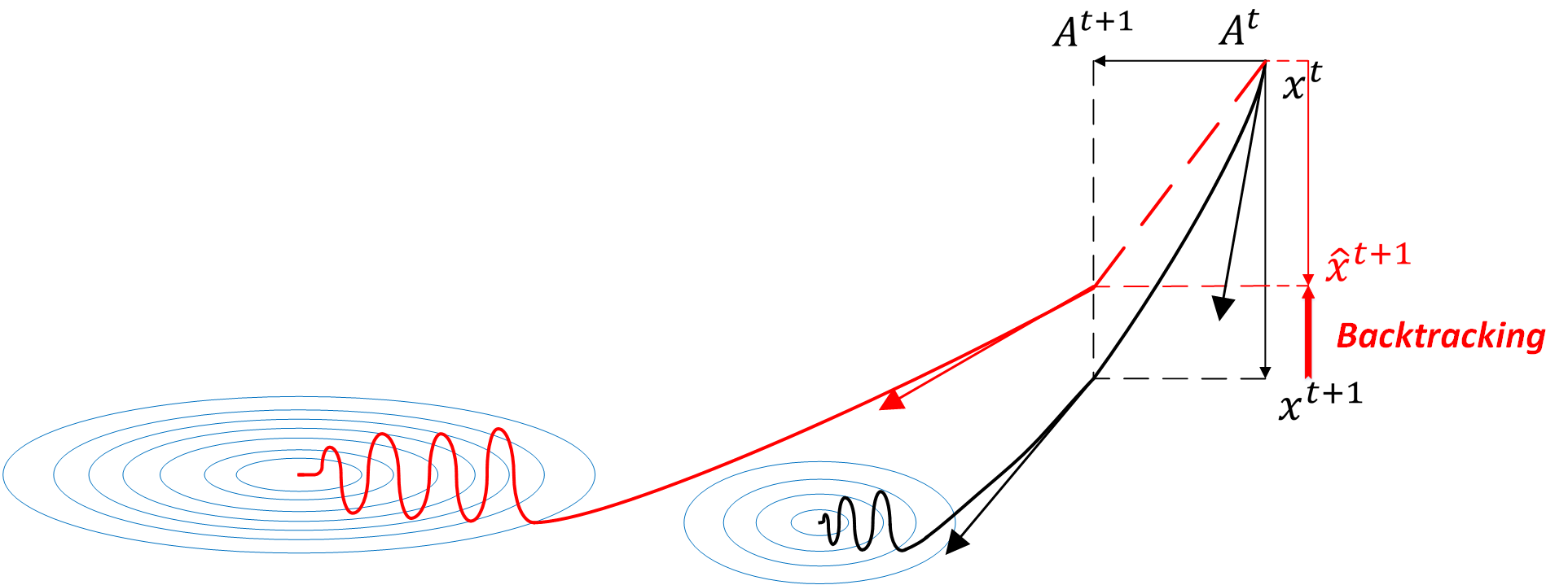
Figure 1: CoGradient Descent (CoGD) drives the optimization escaping from local minima by backtracking (projecting) the current solution to its previous positions based on a projection function.

Existing methods tend to decompose the bilinear optimization problem into manageable sub-problems, and solve them using the Alternating Direction Method of Multipliers (ADMM)  Heide et al. (2015); Yang et al. (2017a) . Without considering the relationship between two hidden factors, however, existing methods suffer from sub-optimal solutions caused by an asynchronous convergence speed of the hidden variables. The variable with the sparsity constraint can converge faster than the variables without the sparsity constraint, which causes insufficient training since the optimization with less active variables is more likely to fall into the local minima. In terms of the convergence speed, the interaction between different variables is seldom explored in the literature so that the collaborative or dependable nature of different variables for optimization is neglected, leading to a sub-optimal solution. As shown in Fig. 2, we backtrack the sparse variable that will be collaborating again with other variables to facilitate the escape from local minima and pursuing optimal solutions for complex tasks.

In this paper, we introduce a Cogradient Descent algorithm (CoGD) for dependable learning on bilinear models, and target the asynchronous gradient descent problem by considering its coupled relationship with other variables. CoGD is formulated as a general framework where the coupling between hidden variables can be used to coordinate the gradients based on a kernelized projection function. Based on CoGD, the variables are sufficiently trained and decoupled to improve the training process. As shown in Zhang K (2018), the resulting decoupling variables can enhance the causality of the learning system. CoGD is applied to representative bilinear problems with one variable having a sparsity constraint, which is widely used in the learning paradigm. The contributions of this work are summarized as follows:

• We propose a dependable learning based on Cogradient Descent (CoGD) algorithm to better solve the bilinear optimization, creating a solid theoretical framework to coordinate the gradient of hidden variables based on a kernelized projection function.

• We propose an optimization strategy that considers the interaction of variables in bilinear optimization, and solve the asynchronous convergence with gradient-based learning procedures.

• Extensive experiments demonstrate that CoGD achieves significant performance improvements on typical bilinear problems including convolutional sparse coding (CSC), network pruning, and CNN training.

This work is an extension of our CVPR paper Zhuo et al. (2020) by providing the details of the derivation of our theoretical model, which leverages a kernelized projection function to reveal the interaction of the variables in terms of convergence speed. In addition, more extensive experiments including CNN model training are conducted to validate the effectiveness of the proposed algorithm.

2 Related Work

Gradient Descent. Gradient descent plays one of the essential roles in the optimization of differentiable models, by pursuing a solution for an objective function to minimize the cost function, as far as possible. It starts from an initial state that is iteratively updated by the opposite partial derivative with respect to the current input. Variations in the gradient update method lead to different versions of gradient descent, such as Momentum, Adaptive Moment Estimation Kingma and Ba (2014), Nesterov accelerated gradient Dozat (2016), and Adagrad Zeiler (2012).

In the deep learning era, with large-scale dataset, stochastic gradient descent (SGD) and its variants are practical choices. Unlike vanilla gradient descent which performs the update based on the entire training set, SGD can work well using solely a small part of the training data. SGD is generally termed batch SGD and allows the optimizer converge to minima or local minima based on gradient descent. There are some related literature Goldt et al. (2019) which discuss the dynamic properties of SGD for deep neural networks. These dynamics and their performance are investigated in the teacher-student setup using SGD, which shows how the dynamics of SGD are captured by a set of differential equations. It also indicates that achieving good generalization in neural networks goes beyond the properties of SGD alone and depends on the interplay of the algorithm, the model architecture, and the data distribution.

Convolutional Sparse Coding. Convolutional sparse coding (CSC) is a classic bilinear optimization problem and has been exploited for image reconstruction and inpainting. Existing algorithms for CSC tend to split the bilinear optimization problem into subproblems, each of which is iteratively solved by ADMM. Fourier domain approaches Bristow et al. (2013); Wohlberg (2014) are also exploited to solve the $\ell_{1}$ regularization sub-problem using soft thresholding. Furthermore, recent works  Heide et al. (2015); Yang et al. (2017a) split the objective into a sum of convex functions and introduce ADMM with proximal operators to speed up the convergence. Although the generalized bilinear model Yokoya et al. (2012) considers a nonlinear combination of several end members in one matrix (not two bilinear matrices), it only proves to be effective in unmixing hyperspectral images. These approaches simplify bilinear optimization problems by regarding the two factors as independent and optimizing one variable while keeping the other unchanged.

Bilinear Models in Deep Learning. Bilinear models can be embedded in CNNs. One application is network pruning, which is one of the hottest topics in the deep learning community Lin et al. (2019, 2020); liu2017Learning. With the aid of bilinear models, the important feature maps and corresponding channels are pruned  liu2017Learning. Bilinear based network pruning can be performed by iterative methods like modified the Accelerated Proximal Gradient (APG) Huang and Wang (2018a) and the iterative shrinkage-thresholding algorithm (ISTA) Ye et al. (2018); Lin et al. (2019). A number of deep learning applications, such as fine-grained categorization Lin et al. (2015); Li et al. (2017), visual question answering (VQA) Yu et al. (2017) and person re-identification Suh et al. (2018), attempt to embed bilinear models into CNNs to model pairwise feature interactions and fuse multiple features with attention. To update the parameters, they directly utilize the gradient descent algorithm and back-propagate the gradients of the loss.

An interesting application of CoGD is studied in CNNs learning. Considering the linearity of the convolutional operation, CNN training can also be considered as a bilinear optimization task as

$$F_{j}^{l+1}=f(BN(\sum\limits_{i}{F_{i}^{l}\otimes W_{{{i,j}}}^{l}})),$$ (2)

where $F_{j}^{l}$ and $F_{j}^{l+1}$ are the $i$-th input and the $j$-th output feature maps at the $l$-th and $(l+1)$-th layer, $W^{l}_{i,j}$ are convolutional filters, and $\otimes$, $BN(\cdot)$ and $f(\cdot)$ refer to convolutional operator, batch normalization and activation respectively. However, the convolutional operation is not as efficient as a traditional bilinear model. We instead consider a batch normalization (BN) layer to validate our method, which can be formulated as a bilinear optimization problem as detailed in Section 4.2. We use the CoGD to replace SGD to efficiently learn the CNN, with the aim to validate the effectiveness of the proposed method.

Figure 2: An illustration of CoGD. Conventional gradient-based algorithms have a heuristic that the two hidden variables in bilinear models are independent. Nevertheless, we validate that such a heuristic is implausible, and the algorithms suffer from asynchronous convergence and sub-optimal solutions. The red dotted lines denote that the sparsity of $\mathbf{x}$ causes an inefficient training of $\mathbf{A}$. We propose a projection function to coordinate the gradient of the hidden variables.

3 The Proposed Method

The proposed method considers the relationship between two variables with the benefits on the linear inference. It is essentially different from previous bilinear models which typically optimize one variable while keeping the other unchanged. In what follows, we first discuss the gradient varnishing problem in bilinear models and then present CoGD.

3.1 Gradient Descent

Assuming $\mathbf{A}$ and $\mathbf{x}$ are independent, the conventional gradient descent method can be used to solve the bilinear optimization problem as

$$\mathbf{A}^{t+1}=\mathbf{A}^{t}+\eta_{1}\frac{\partial G}{\partial\mathbf{A}},$$ (3)

where

$$(\frac{\partial G}{\partial\mathbf{A}})^{T}=\mathbf{x}^{t}(\mathbf{A}\mathbf{x}^{t}-\mathbf{b})^{T}=\mathbf{x}^{t}\hat{G}(\mathbf{A},\mathbf{x}).$$ (4)

The function $\hat{G}$ is defined by considering the bilinear optimization problem as in Eq. 1, and we have

$$\hat{G}(A,x)=(\mathbf{A}\mathbf{x}^{t}-\mathbf{b})^{T}.$$ (5)

Eq. 4 shows that the gradient for $\mathbf{A}$ tends to vanish, when $\mathbf{x}$ approaches zero due to the sparsity regularization term $||x||_{1}$. Although it has a chance to be corrected in some tasks, more likely, the update will cause an asynchronous convergence. Note that for simplicity, the regularization term on $A$ is not considered. Similarly, for $\mathbf{x}$, we have

$$\mathbf{x}^{t+1}=\mathbf{x}^{t}+\eta_{2}\frac{\partial G}{\partial\mathbf{x}}.$$ (6)

$\eta_{1}$ and $\eta_{2}$ are the learning rates. The conventional gradient descent algorithm for bilinear models iteratively optimizes one variable while keeping the other fixed. This unfortunately ignore the relationship of the two hidden variables in optimization.

3.2 Cogradient Descent for Dependable Learning

We consider the problem from a new perspective such that $\mathbf{A}$ and $\mathbf{x}$ are coupled. Firstly, based on the chain rule Petersen et al. (2008) and its notations, we have

$$\hat{x}^{t+1}_{j} ={x}^{t}_{j}+\eta_{2}(\frac{\partial G}{\partial x_{j}}+Tr((\frac{\partial{G}}{\partial\mathbf{A}})^{T}\frac{\partial{\mathbf{A}}}{\partial x_{j}})),$$ (7)

where $(\frac{\partial G}{\partial\mathbf{A}})^{T}=\mathbf{x}^{t}\hat{G}(\mathbf{A},\mathbf{x})$ as shown in Eq. 4. $Tr(\cdot)$ represents the trace of the matrix, which means that each element in the matrix $\frac{\partial G}{\partial x_{j}}$ adds the trace of the corresponding matrix related to $x_{j}$. Considering

$$\frac{\partial G}{\partial\mathbf{A}}=\mathbf{A}\mathbf{x}^{t}\mathbf{x}^{T,t}-b\mathbf{x}^{T,t},$$ (8)

we have

$$\frac{\partial G(\mathbf{A})}{\partial x_{j}} =Tr[(\mathbf{A}\mathbf{x}^{t}\mathbf{x}^{T,t}-b\mathbf{x}^{T,t})^{T}\frac{\partial\mathbf{A}}{\partial x_{j}}]$$ (9)

$$=Tr[((\mathbf{A}\mathbf{x}^{t}-b)\mathbf{x}^{T,t})^{T}]\frac{\partial\mathbf{A}}{\partial x_{j}}$$

$$=Tr[\mathbf{x}^{t}\hat{G}\frac{\partial\mathbf{A}}{\partial x_{j}}],$$

where $\hat{G}=(\mathbf{A}\mathbf{x}^{t}-b)^{T}=[\hat{g}_{1},...,\hat{g}_{M}]$. Supposing that $\mathbf{A}_{i}$ and $x_{j}$ are independent when $i\neq j$, we have

$$\frac{\partial\mathbf{A}}{\partial x_{j}}=\begin{bmatrix}0&...&\frac{\partial\mathbf{A}_{1j}}{\partial x_{j}}&...&0\\ .&&.&&.\\ .&&.&&.\\ .&&.&&.\\ 0&...&\frac{\partial\mathbf{A}_{Mj}}{\partial x_{j}}&...&0\end{bmatrix},$$ (10)

and

$$\mathbf{x}\hat{G}=\begin{bmatrix}x_{1}\hat{g}_{1}&...&x_{1}\hat{g}_{j}&...&x_{1}\hat{g}_{M}\\ .&&.&&.\\ .&&.&&.\\ .&&.&&.\\ x_{N}\hat{g}_{1}&...&x_{N}\hat{g}_{j}&...&x_{N}\hat{g}_{M}\end{bmatrix}.$$ (11)

Combining Eq. 10 and Eq. 11, we have

$$\mathbf{x}\hat{G}\frac{\partial\mathbf{A}}{\partial x_{j}}=\begin{bmatrix}0&...&x_{1}\sum_{i}^{M}\hat{g}_{i}\frac{\partial\mathbf{A}_{ij}}{\partial x_{j}}&...&0\\ .&&.&&.\\ .&&.&&.\\ .&&.&&.\\ 0&...&x_{N}\sum_{i}^{M}\hat{g}_{i}\frac{\partial\mathbf{A}_{ij}}{\partial x_{j}}&...&0\end{bmatrix}.$$ (12)

The trace of Eq. 12 is then calculated by:

$$Tr[\mathbf{x}^{t}\hat{G}\frac{\partial\mathbf{A}}{\partial x_{j}}]=x_{j}\sum_{i}^{M}\hat{g}_{i}\frac{\partial\mathbf{A}_{ij}}{\partial x_{j}}.$$ (13)

Remembering that $\mathbf{x}^{t+1}=\mathbf{x}^{t}+\eta_{2}\frac{\partial G}{\partial\mathbf{x}}$, CoGD is established by combining Eq. 7 and Eq. 13:

$$\hat{\mathbf{x}}^{t+1} =\mathbf{x}^{t+1}+\eta_{2}\begin{bmatrix}\sum_{i}^{M}\hat{g}_{i}\frac{\partial\mathbf{A}_{i1}}{\partial x_{1}}\\ .\\ .\\ .\\ \sum_{i}^{M}\hat{g}_{i}\frac{\partial\mathbf{A}_{iN}}{\partial x_{N}}\end{bmatrix}\odot\begin{bmatrix}x_{1}\\ .\\ .\\ .\\ x_{N}\end{bmatrix}$$ (14)

$$=\mathbf{x}^{t+1}+\eta_{2}\begin{bmatrix}<\hat{G},\frac{\partial\mathbf{A}_{1}}{\partial x_{1}}>\\ .\\ .\\ .\\ <\hat{G},\frac{\partial\mathbf{A}_{N}}{\partial x_{N}}>\end{bmatrix}\odot\begin{bmatrix}x_{1}\\ .\\ .\\ .\\ x_{N}\end{bmatrix}$$

$$=\mathbf{x}^{t+1}+\eta_{2}{\mathbf{c}}\odot\mathbf{x}^{t}.$$

We further define the kernelized version of $\mathbf{c}$, and have

$${\mathbf{c}}=\begin{bmatrix}\hat{K}(\hat{G},\frac{\partial\mathbf{A}_{1}}{\partial x_{1}})\\ .\\ .\\ .\\ \hat{K}(\hat{G},\frac{\partial\mathbf{A}_{N}}{\partial x_{N}})\end{bmatrix},$$ (15)

where $\hat{K}(.,.)$ is a kernel function. Remembering that Eq. 6, $\mathbf{x}^{t+1}=\mathbf{x}^{t}+\eta_{2}\frac{\partial G}{\partial\mathbf{x}}$, Eq. 7 then becomes

$$\hat{\mathbf{x}}^{t+1}=\mathbf{x}^{t+1}+\eta_{2}\mathbf{c}^{t}\odot\mathbf{x}^{t},$$ (16)

where $\odot$ represents the Hadamard product. It is then reformulated as a projection function as

$$\hat{\mathbf{x}}^{t+1}=P(\mathbf{x}^{t+1},\mathbf{x}^{t})=\mathbf{x}^{t+1}+\beta\odot\mathbf{x}^{t},$$ (17)

which shows the rationality of our method, $i.e.$, it is based on a projection function to solve the asynchronous problem of the bilinear optimization by controlling $\beta$.

We first judge when an asynchronous convergence happens in the optimization based on a form of logical operation as

$$(\neg s(\mathbf{x}))\wedge(s(\mathbf{A}))=1,$$ (18)

and

$$s(*)=\begin{cases}1&if\ R(*)\ \geq\alpha,\\ 0&otherwise,\end{cases}$$ (19)

where $\alpha$ represents the threshold which changes for different applications. Eq. 18 describes an assumption that an asynchronous convergence happens for $\mathbf{A}$ and $\mathbf{x}$ when their norms become significantly different. Accordingly, the update rule of the proposed CoGD is defined as

$$\hat{\mathbf{x}}^{t+1}=\begin{cases}P(\mathbf{x}^{t+1},\mathbf{x}^{t})&if\ (\neg s(\mathbf{x}))\wedge(s(\mathbf{A}))=1,\\ \mathbf{x}^{t+1}&otherwise,\end{cases}$$ (20)

which leads to a synchronous convergence and generalizes the conventional gradient descent method. CoGD is then established.

Note that $c$ in Eq. 14 is calculated based on $\hat{G}$, which differs for applications. $\frac{\partial\mathbf{A}_{j}}{\partial{x_{j}}}\approx\frac{\Delta\mathbf{A}_{j}}{\Delta x_{j}}$, where $\Delta$ denotes the difference of the variable over the epoch related to the convergence speed. $\frac{\partial\mathbf{A}_{j}}{\partial{x_{j}}}=\mathbf{1}$, if $\Delta x_{j}$ or $x_{j}$ approaches to zero. With above derivation, we define CoGD within the gradient descent framework, providing a solid foundation for the convergence analysis of CoGD. Based on CoGD, the variables are sufficiently trained and decoupled, which can enhance the causality of the learning system Zhang K (2018).

4 Applications

We apply the proposed algorithm on Convolutional Sparse Coding (CSC), deep learning to validate its general applicability to bilinear problems including image inpainting, image reconstruction, network pruning and CNN model training.

4.1 Convolutional Sparse Coding

CSC operates on the whole image, decomposing a global dictionary and set of features. The CSC problem theoretically more challenging than the patch-based sparse coding Mairal et al. (2010) and requires more sophisticated optimization model. The reconstruction process is usually based on a bilinear optimization model formulated as

$$\mathop{\arg\min}\limits_{\mathbf{A},\mathbf{x}} \frac{1}{2}\left\|\mathbf{b}-\mathbf{A}\mathbf{x}\right\|^{2}_{F}+\lambda\left\|\mathbf{x}\right\|_{1}$$ (21)

s.t. $$\left\|\mathbf{A}_{k}\right\|^{2}_{2}\leq 1\quad\forall k\in\{1,\dots,K\},$$

where $\mathbf{b}$ denotes input images.

$\mathbf{x}=[\mathbf{x}_{1}^{T},\dots,\mathbf{x}_{K}^{T}]^{T}$ denotes coefficients under sparsity regularization. $\lambda$ is the sparsity regularization factor. $\mathbf{A}=[\mathbf{A}_{1},\dots,\mathbf{A}_{K}]$ is a concatenation of Toeplitz matrices representing the convolution with the kernel filters $\mathbf{A}_{k}$, where $K$ is the number of the kernels.

In Eq. 21, the optimized objectives or models are influenced by two or more hidden factors that interact to produce the observations. Existing solution tend to decompose the bilinear optimization problem into manageable sub-problems Parikh et al. (2014); Heide et al. (2015). Without considering the relationship between two hidden factors, however, existing methods suffer from sub-optimal solutions caused by an asynchronous convergence speed of the hidden variables. We attempt to purse an optimized solution based on the proposed CoGD.

Specifically, we introduce a diagonal or block-diagonal matrix $\mathbf{m}$ to the sparse coding framework defined in  Gu et al. (2015) and reformulate Eq. 21 as

$$\mathop{\arg\min}\limits_{\mathbf{A},\mathbf{x}}f_{1}(\mathbf{A}\mathbf{x})+\sum_{k=1}^{K}(f_{2}(\mathbf{x}_{k})+f_{3}(\mathbf{A}_{k})),$$ (22)

where

$$f_{1}(\mathbf{v}) =\frac{1}{2}\left\|\mathbf{b}-\mathbf{m}\mathbf{v}\right\|_{F}^{2},$$ (23)

$$f_{2}(\mathbf{v}) =\lambda\left\|\mathbf{v}\right\|_{1},$$

$$f_{3}(\mathbf{v}) =ind_{c}(\mathbf{v}).$$

In Eq. 23, $ind_{c}(\cdot)$ is an indicator function defined on the convex set of the constraints $C=\{\mathbf{x}|\left\|\mathbf{Sx}\right\|_{2}^{2}\leq 1\}$. Similar to Eq. 20, we have

$$\ \ \ \ \ \ \hat{\mathbf{x}}_{k}=\begin{cases}P({\mathbf{x}}^{t+1}_{k},{\mathbf{x}}^{t}_{k})&if\ (\neg s(\mathbf{x}_{k}))\wedge(s(\mathbf{A}_{k}))=1\\ {\mathbf{x}}^{t+1}_{k}&otherwise\end{cases},$$ (24)

which solve the two coupled variables iteratively, yielding a new CSC solution as defined in Alg. 1. $P({\mathbf{x}}^{t+1}_{k},{\mathbf{x}}^{t}_{k})$ is calculated based on $\hat{G}(\mathbf{A},\mathbf{x})$, which is defined in Eq. 5.

Algorithm 1 CoGD for CSC.

0:  The training dataset; sparsity factor $\lambda$; hyperparameters such as penalty parameters, threshold $\alpha_{\mathbf{a}}$, $\alpha_{\mathbf{x}}$.

0:  The filters $\mathbf{a}$ and the sparse feature maps $\mathbf{x}$.

1:  Initialize $\mathbf{a}^{0},\mathbf{x}^{0}$ and others

2:  repeat

3:     Use $f_{3}({\mathbf{a}_{k}})$ in Eq. 23 to calculate kernel norm

4:     Use Eq. 24 to calculate $\mathbf{x}$

5:     for all $l=1$ to $L$ epochs do

6:        Kernel Update:$\mathbf{a}^{l}$ $\leftarrow\mathop{\arg\min}\limits_{\mathbf{a}}f_{1}(\mathbf{a}\mathbf{x})+\sum_{k=1}^{K}f_{3}(\mathbf{a}_{k})$ using ADMM with proximal operators

7:        Code Update:$\mathbf{x}^{l}$ $\leftarrow\mathop{\arg\min}\limits_{\mathbf{x}}f_{1}(\mathbf{a}\mathbf{x})+\sum_{k=1}^{K}f_{2}(\mathbf{x}_{k})$ using ADMM with proximal operators

8:     end for

9:  until Loss convergence.

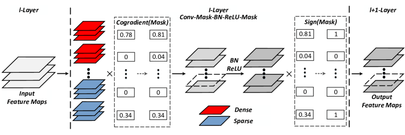
Figure 3: The forward process with the soft mask.

4.2 Network Pruning

Network pruning, particularly convolutional channel pruning, has received increased attention for compressing CNNs. Early works in this area tended to directly prune the kernel based on simple criteria like the norm of kernel weights Li et al. (2016) or use a greedy algorithm Luo et al. (2017). Recent approaches have formulated network pruning as a bilinear optimization problem with soft masks and sparsity regularization He et al. (2017); Ye et al. (2018); Huang and Wang (2018a); Lin et al. (2019).

Based on the framework of channel pruning He et al. (2017); Ye et al. (2018); Huang and Wang (2018a); Lin et al. (2019), we apply the proposed CoGD for network pruning. To prune a channel of the network, the soft mask $\mathbf{m}$ is introduced after the convolutional layer to guide the output channel pruning. This is defined as a bilinear model as

$$F_{j}^{l+1}=f(\sum\limits_{i}{F_{i}^{l}\otimes(W_{{{i,j}}}^{l}}{\mathbf{m}_{j}})),$$ (25)

where $F_{j}^{l}$ and $F_{j}^{l+1}$ are the $i$-th input and the $j$-th output feature maps at the $l$-th and $(l+1)$-th layer. $W^{l}_{i,j}$ are convolutional filters corresponding to the soft mask $\mathbf{m}$. $\otimes$ and $f(\cdot)$ respectively refer to convolutional operator and activation.

Algorithm 2 CoGD for Pruning CNNs in Bilinear Modeling.

0:  The training dataset; the pre-trained network with weights $W_{B}$; sparsity factor $\lambda$; hyperparameters such as learning rate, weight decay, threshold $\alpha_{W}$, $\alpha_{\mathbf{m}}$.

0:  The pruning network.

1:  Initialize $W_{G}=W_{B}$, $\mathbf{m}\sim N(0,1)$;

2:  repeat

3:     Use $R(W_{G})$ in Eq. 26 to obtain the norms

4:     Use Eq. 27 to calculate the new soft mask $\hat{\mathbf{m}}$

5:     for all $l=1$ to $L$ epochs do

6:        for all $i$ steps do

7:           Fix $W_{G}$ and update $W_{D}$ using Eq. 29

8:        end for

9:        for all $j$ steps do

10:           Fix $W_{D}$ and update $W_{G}$ using Eq. 29

11:        end for

12:     end for

13:  until Loss convergence.

In this framework shown in Fig. 3, the soft mask $\mathbf{m}$ is learned end-to-end in the back propagation process. To be consistent with other pruning works, we use $W$ and $\mathbf{m}$ instead of $\mathbf{A}$ and $\mathbf{x}$. A general optimization function for network pruning with a soft mask is defined as

$$\mathop{\arg\min}\limits_{W,\mathbf{m}}\mathcal{L}(W,{\mathbf{m}})+\lambda{\left\|\mathbf{m}\right\|_{1}}+R({W}),$$ (26)

where $\mathcal{L}(W,{\mathbf{m}})$ is the loss function, described in details below. With the sparsity constraint on $\mathbf{m}$, the convolutional filters with zero value in the corresponding soft mask are regarded as useless filters. This means that these filters and their corresponding channels in the feature maps have no significant contribution to the network predictions and should be pruned. There is, however, a dilemma in the pruning-aware training in that the pruned filters are not evaluated well before they are pruned, which leads to sub-optimal pruning. In particular, the soft mask $\mathbf{m}$ and the corresponding kernels are not sparse in a synchronous manner, which can prune the kernels still of potentials. To address this problem, we apply the proposed CoGD to calculate the soft mask $\mathbf{m}$, by reformulating Eq. 20 as

$$\hat{\mathbf{m}}^{l,t+1}_{j}\!= \begin{cases}P({\mathbf{m}_{j}}^{l,t+1},{\mathbf{m}_{j}}^{l,t})&if\ (\neg s(\mathbf{m}_{j}^{l,t}))\wedge s(\sum_{i}W_{i,j}^{l})\!=\!1\\ {\mathbf{m}}^{l,t+1}_{j}&otherwise,\end{cases}$$ (27)

where $W_{i,j}$ represents the 2D kernel of the $i$-th input channel of the $j$-th filter. $\beta$, $\alpha_{W}$ and $\alpha_{\mathbf{m}}$ are detailed in experiments. The form of $\hat{G}$ is specific for different applications. For CNN pruning, based on Eq. 4, we simplify the calculation of $\hat{G}$ as

$$\hat{G}=\frac{\partial\mathcal{L}}{\partial W_{i,j}}/\mathbf{m}_{j}.$$ (28)

Note that the the autograd package in deep learning frameworks such as Pytorch Paszke et al. (2019) can automatically calculate $\frac{\partial\mathcal{L}}{\partial W_{i,j}}$. We then Substitute Eq. 28 into Eq. 15 to train our network, and prune CNNs based on the new mask $\hat{\mathbf{m}}$ in Eq. 27.

To examine how our CoGD works for network pruning, we use GAL Lin et al. (2019) as an example to describe our CoGD for CNN pruning. A pruned network obtained through GAL with $\ell_{1}$-regularization on the soft mask is used to approximate the pre-trained network by aligning their outputs. The discriminator $D$ with weights $W_{D}$ is introduced to discriminate between the output of the pre-trained network and the pruned network. The pruned network generator $G$ with weights $W_{G}$ and soft mask $\mathbf{m}$ is learned together with $D$ by using the knowledge from supervised features of the baseline. Accordingly, the soft mask $\mathbf{m}$, the new mask $\hat{\mathbf{m}}$, the pruned network weights $W_{G}$, and the discriminator weights $W_{D}$ are simultaneously learned by solving the optimization problem as follows:

$$\arg\mathop{\min}\limits_{{W_{G}},\mathbf{m}}\mathop{\max}\limits_{{W_{D}},\hat{\mathbf{m}}} {\mathcal{L}_{Adv}}({W_{G}},\hat{\mathbf{m}},{W_{D}})+{\mathcal{L}_{data}}({W_{G}},\hat{\mathbf{m}})$$ (29)

$$+ {\mathcal{L}_{reg}}({W_{G}},\mathbf{m},{W_{D}}).$$

where $\mathcal{L}(W,{\mathbf{m}})={\mathcal{L}_{Adv}}({W_{G}},\hat{\mathbf{m}},{W_{D}})+{\mathcal{L}_{data}}({W_{G}},\hat{\mathbf{m}})$ and ${\mathcal{L}_{reg}}({W_{G}},\mathbf{m},{W_{D}})$ are related to $\lambda{\left\|\mathbf{m}\right\|_{1}}+R({W})$ in Eq. 26. ${\mathcal{L}_{Adv}}({W_{G}},\hat{\mathbf{m}},{W_{D}})$ is the adversarial loss to train the two-player game between the pre-trained network and the pruned network that compete with each other. Details of the algorithm are described in Alg. 2.

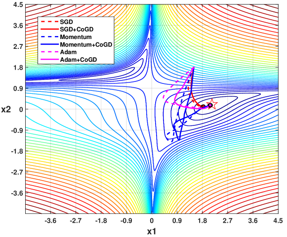
Figure 4: Comparison of classical gradient algorithm with CoGD.The background is the contour map of Beale functions. The algorithms with CoGD have short optimization paths compared with their counterparts, which shows that CoGD facilitates efficient and sufficient training.

The advantages of CoGD in network pruning are three-fold. First, CoGD that optimizes the bilinear pruning model leads to a synchronous gradient convergence. Second, the process is controllable by a threshold, which makes the pruning rate easy to adjust. Third, the CoGD method for network pruning is scalable, $i.e.$, it can be built upon other state-of-the-art networks for better performance.

4.3 CNN Training

The last but not the least, CoGD can be fused with the Batch Normalization (BN) layer and improve the performance of CNN models. As is known, the BN layer can re-distribute the features, resulting that the feature and kernel learning converge in an asynchronous manner. CoGD is then introduced to synchronize their learning speeds to sufficiently train CNN models. In specific, we backtrack sparse convolutional kernels through evaluating the sparsity of the BN layer, leading to an efficient training process. To ease presentation, we first copy Eq. 2 as

$$F_{j}^{l+1}=f(BN(\sum\limits_{i}{F_{i}^{l}\otimes W_{{{i,j}}}^{l}})),,$$ (30)

then redefine the BN model as

$$BN(x)=\gamma\frac{x-\mu_{B}}{\sqrt{\sigma_{B}+\epsilon}}+\beta,$$ (31)

$$\mu_{B}=\frac{1}{m}\sum_{i=1}^{m}{x_{i}},$$

$$\sigma_{B}=\frac{1}{m}\sum_{i=1}^{m}(x_{i}-\mu_{B})^{2},$$

where $m$ is the mini-batch size, $\mu_{B}$ and $\sigma_{B}$ are mean and variance obtained by feature calculation in the BN layer. $\gamma$ and $\beta$ are the learnable parameters, and $\epsilon$ is a small number to avoid dividing by zero.

According to Eq. 30 and Eq. 31, we can easily know that $\gamma$ and $W$ are bilinear. We use the sparsity of $\gamma$ instead of the whole convolutional features for kernels backtracking, which simplifies the operation and improves the backtracking efficiency. Similar to network pruning, we also use $\gamma$ and $W$ instead of $\mathbf{A}$ and $\mathbf{x}$ in this part. A general optimization for CNN training with the BN layer as

$$\mathop{\arg\min}\limits_{W,\gamma}\mathcal{L}(W,\gamma)+\lambda{\left\|W\right\|_{1}},$$ (32)

where $\mathcal{L}(W,\gamma)$ is the loss function defined on Eq. 30 and Eq. 31. CoGD is then applied to train CNNs, by reformulating Eq. 20 as

$$\hat{W}^{l,t+1}_{i,j}\!= \begin{cases}P({W_{i,j}}^{l,t+1},{W_{i,j}}^{l,t})&if\ (\neg s(\gamma_{j}^{l}))\wedge s(\sum_{i}W_{i,j}^{l})\!=\!1\\ {W_{i,j}}^{l,t}&otherwise,\end{cases}$$ (33)

where $\gamma_{j}^{l}$ is the $j$-th learnable parameter in the $l$-th BN layer. $W_{i,j}$ represents the 2D kernel of the $i$-th input channel of the $j$-th filter. Similar to network pruning, we define

$$\hat{G}=\frac{\partial\mathcal{L}}{\partial W_{i,j}}/\mathbf{\gamma}_{j},$$ (34)

where $\frac{\partial\mathcal{L}}{\partial W_{i,j}}$ is obtained based on the autograd package in deep learning frameworks such as Pytorch Paszke et al. (2019). Similar to network pruning, we substitute Eq. 34 into Eq. 15, to use CoGD for CNN training, yielding Alg. 3.

Algorithm 3 CoGD for the CNN model training.

0:  The training dataset; sparsity factor $\lambda$; hyperparameters such as learning rate, weight decay, threshold $\alpha_{W}$, $\alpha_{\mathbf{m}}$.

0:  CNN Model.

1:  Initialize and define the loss function (Eq. 32) with sparsity constraint on the kernel $W$;

2:  repeat

3:     Use Eq. 30 to define the BN layer to get a bilinear model

4:     for all $l=1$ to $L$ epochs do

5:        Calculate $\hat{G}$ based on Eq. 34

6:        Update $W$ based on Eq. 33 and Eq. 18 using $\alpha_{W}$, $\alpha_{\mathbf{m}}$

7:        Update other parameters based on the autograd package in the Pytorch deep learning framework

8:     end for

9:  until Loss convergence.

5 Experiments

In this section, CoGD is first analyzed and compared with classical optimization methods on a baseline problem. It is then validated on the problems of CSC, network pruning, and CNN model training.

5.1 Baseline Problem

A baseline problem is first used as an example to illustrate the superiority of our algorithm. The problem is the optimization of Beale function under constraint of $F(x_{1},x_{2})=beale(x_{1},x_{2})+\left\|x_{1}\right\|+x_{2}^{2}$. The Beale function has the same form as Eq. 1 and can be regraded as a bilinear optimization problem with respect to variables $x_{1}x_{2}$. During optimization, the learning rate $\eta_{2}$ is set as $0.001$, $0.005$, $0.1$ for ‘SGD’, ‘Momentum’ and ‘Adam’ respectively. The thresholds $\alpha_{x_{1}}$ and $\alpha_{x_{2}}$ for CoGD are set to $1$ and $0.5$. $\beta=0.001\eta_{2}\mathbf{c}^{t}$ with $\frac{\partial x_{2}}{\partial{x_{1}}}\approx\frac{\Delta x_{2}}{\Delta x_{1}}$, where $\Delta$ denotes the difference of variable over the epoch. $\frac{\Delta x_{2}}{\Delta x_{1}}=\mathbf{1}$, when $\Delta x_{2}$ or $x_{2}$ approaches zero. The total number of iterations is $200$.

In Fig. 4, we compare the optimization paths of CoGD with those of three widely used optimization methods - ‘SGD’, ‘Momentum’ and ‘Adam’. It can be seen that algorithms equipped with CoGD have shorter optimization paths than their counterparts. Particularly, the ADAM-CoGD algorithm has a much shorter path than ADAM, demonstrating the fast convergence of the proposed CoGD algorithm. The similar convergence with shorter paths means that CoGD facilitates efficient and sufficient training.

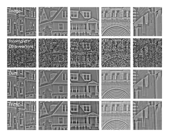
Figure 5: Inpainting for the normalized city dataset. From top to bottom: the original images, incomplete observations, reconstructions with FFCSC Heide et al. (2015), and reconstructions with our proposed algorithm.

5.2 Convolutional Sparse Coding

Experimental Setting. The CoGD for convolutional sparse coding (CSC) is evaluated on two public datasets: the fruit dataset Zeiler et al. (2010) and the city dataset Zeiler et al. (2010); Heide et al. (2015), each of which consists of ten images with 100 $\times$ 100 resolution. To evaluate the quality of the reconstructed images, we use two standard metrics, the peak signal-to-noise ratio (PSNR, unit:dB) and the structural similarity (SSIM). The higher the PSNR and the SSIM values are, the better the visual quality of the reconstructed image is. The evaluation metrics are defined as:

$$PSNR=10\times\log_{10}(\frac{MAX^{2}}{MSR}),$$ (35)

where $MSE$ is the mean square error of clean image and noisy image. $MAX$ is the maximum pixel value of the image.

$$SSIM(x,y)=\frac{(2\mu_{x}\mu_{y}+C_{1})(2\sigma_{xy}+C_{2})}{(mu_{x}^{2}+\mu_{y}^{2}+C_{1})(\sigma_{x}^{2}+\sigma_{y}^{2}+C_{2})},$$ (36)

where $\mu$ is the mean of samples. $\sigma$ is the variance of samples. $\sigma_{xy}$ is the covariance of the samples. $C$ is a constant, $C_{1}=(0.01\times MAX)^{2}$, $C_{2}=(0.03\times MAX)^{2}$

Implementation Details: The reconstruction model is implemented based on the conventional CSC method Gu et al. (2015), while we introduce the CoGD with the kernelized projection function to achieve a better convergence and higher reconstruction accuracy. One hundred of filters with size 11$\times$11 are set as model parameters. $\alpha_{\mathbf{x}}$ is set to the mean of $\left\|\mathbf{x}_{k}\right\|_{1}$. $\alpha_{\mathbf{A}}$ is calculated as the median of the sorted results of $\beta_{k}$. As shown in Eq. 15, linear and polynomial kernel functions are used in the experiment, which can both improve the performance of our method. For a fair comparison, we use the same hyperparameters ($\eta_{2}$) in both our method and Gu et al. (2015). We also test $\beta=0.1\eta_{2}\mathbf{c}^{t}$, which achieves a similar performance as the linear kernel.

Table 1: Inpainting results for convolutional filters learned with the proposed method and with FFCSC Heide et al. (2015). All reconstructions are performed with 75% data subsampling. The proposed CoGD achieves better PSNR and SSIM in all cases.

Dataset	Fruit	1	2	3	4	5	6	7	8	9	10	Average
PSNR (dB)	Heide et al. (2015)	25.37	24.31	25.08	24.27	23.09	25.51	22.74	24.10	19.47	22.58	23.65
	CoGD(kernelized, $k=1$)	26.37	24.45	25.19	25.43	24.91	27.90	24.26	25.40	24.70	24.46	25.31
	CoGD(kernelized, $k=2$)	27.93	26.73	27.19	25.25	23.54	25.02	26.29	24.12	24.48	24.04	25.47
	CoGD(kernelized, $k=3$)	28.85	26.41	27.35	25.68	24.44	26.91	25.56	25.46	24.51	22.42	25.76
SSIM	Heide et al. (2015)	0.9118	0.9036	0.9043	0.8975	0.8883	0.9242	0.8921	0.8899	0.8909	0.8974	0.9000
	CoGD(kernelized, $k=1$)	0.9452	0.9217	0.9348	0.9114	0.9036	0.9483	0.9109	0.9041	0.9215	0.9097	0.9211
	CoGD(kernelized, $k=2$)	0.9483	0.9301	0.9294	0.9061	0.8939	0.9454	0.9245	0.8990	0.9208	0.9054	0.9203
	CoGD(kernelized, $k=3$)	0.9490	0.9222	0.9342	0.9181	0.8810	0.9464	0.9137	0.9072	0.9175	0.8782	0.9168
Dataset	City	1	2	3	4	5	6	7	8	9	10	Average
PSNR (dB)	Heide et al. (2015)	26.55	24.48	25.45	21.82	24.29	25.65	19.11	25.52	22.67	27.51	24.31
	CoGD(kernelized, $k=1$)	26.58	25.75	26.36	25.06	26.57	24.55	21.45	26.13	24.71	28.66	25.58
	CoGD(kernelized, $k=2$)	27.93	26.73	27.19	25.83	24.41	25.31	26.29	24.70	24.48	24.62	25.76
	CoGD(kernelized, $k=3$)	25.91	25.95	25.21	26.26	26.63	27.68	21.54	25.86	24.74	27.69	25.75
SSIM	Heide et al. (2015)	0.9284	0.9204	0.9368	0.9056	0.9193	0.9202	0.9140	0.9258	0.9027	0.9261	0.9199
	CoGD(kernelized, $k=1$)	0.9397	0.9269	0.9433	0.9289	0.9350	0.9217	0.9411	0.9298	0.9111	0.9365	0.9314
	CoGD(kernelized, $k=2$)	0.9498	0.9316	0.9409	0.9176	0.9189	0.9454	0.9360	0.9305	0.9323	0.9284	0.9318
	CoGD(kernelized, $k=3$)	0.9372	0.9291	0.9429	0.9254	0.9361	0.9333	0.9373	0.9331	0.9178	0.9372	0.9329

Table 2: Reconstruction results for filters learned with the proposed method and with FFCSC Heide et al. (2015). With the exception of 6 images, the proposed method achieves better PSNR and SSIM.

Dataset	Fruit	1	2	3	4	5	6	7	8	9	10	Average
PSNR (dB)	Heide et al. (2015)	30.90	29.52	26.90	28.09	22.25	27.93	27.10	27.05	23.65	23.65	26.70
	CoGD(kernelized, $k=1$)	31.46	29.12	27.26	28.80	25.21	27.35	26.25	27.48	25.30	27.84	27.60
	CoGD(kernelized, $k=2$)	30.54	28.77	30.33	28.64	25.72	30.31	28.07	27.46	25.22	26.14	28.12
SSIM	Heide et al. (2015)	0.9706	0.9651	0.9625	0.9629	0.9433	0.9712	0.9581	0.9524	0.9608	0.9546	0.9602
	CoGD(kernelized, $k=1$)	0.9731	0.9648	0.9640	0.9607	0.9566	0.9717	0.9587	0.9562	0.9642	0.9651	0.9635
	CoGD(kernelized, $k=2$)	0.9705	0.9675	0.9660	0.9640	0.9477	0.9728	0.9592	0.9572	0.9648	0.9642	0.9679
Dataset	City	1	2	3	4	5	6	7	8	9	10	Average
PSNR (dB)	Heide et al. (2015)	30.11	27.86	28.91	26.70	27.85	28.62	18.63	28.14	27.20	25.81	26.98
	CoGD(kernelized, $k=1$)	30.29	28.77	28.51	26.29	28.50	30.36	21.22	29.07	27.45	30.54	28.10
	CoGD(kernelized, $k=2$)	30.61	28.57	27.37	27.66	28.57	29.87	21.48	27.08	26.82	29.86	27.79
SSIM	Heide et al. (2015)	0.9704	0.9660	0.9703	0.9624	0.9619	0.9613	0.9459	0.9647	0.9531	0.9616	0.9618
	CoGD(kernelized, $k=1$)	0.9717	0.9660	0.9702	0.9628	0.9627	0.9624	0.9593	0.9663	0.9571	0.9632	0.9642
	CoGD(kernelized, $k=2$)	0.9697	0.9646	0.9681	0.962	0.9613	0.9594	0.9541	0.9607	0.9538	0.9620	0.9631

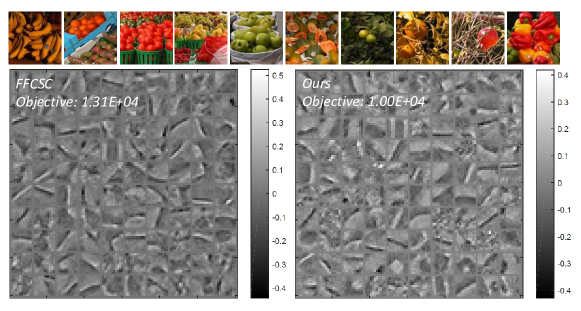
(a)

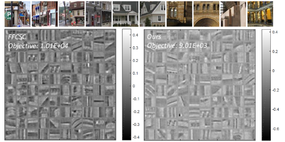
(b)

Figure 6: Filters learned on fruit and city datasets. Thumbnails of the datasets along with filters learned with FFCSC Heide et al. (2015) (left) and with CoGD (right) are shown. The proposed reconstruction method reports lower objectives. (Best viewed in color with zoom)

Results: The CSC with the proposed CoGD algorithm is evaluated with two tasks including image reconstruction and image inpainting.

For image inpainting, we randomly sample the data with a 75% subsampling rate, to obtain the incomplete data. Like Heide et al. (2015), we test our method on contrast-normalized images. We first learn filters from all the incomplete data under the guidance of the soft mask $\mathbf{m}$, and then reconstruct the incomplete data by fixing the learned filters. We show inpainting results of the normalized data in Fig. 5. Moreover, to compare with FFCSC, inpainting results on the fruit and city datasets are shown in Tab. 1. It can be seen that our method achieves a better PSNR and SSIM in all cases while the average PSNR and SSIM improvements are impressive 1.78 db and 0.017.

For image reconstruction, we reconstruct the images on the fruit and city datasets. One hundred of 11$\times$11 filters are trained and compared with those of FFCSC Heide et al. (2015). Fig. 6 shows the resulting filters after convergence within the same 20 iterations. It can be seen that the proposed reconstruction method, driven with CoGD, converges with a lower loss. When comparing the PSNR and the SSIM of our method with FFCSC in Tab. 2, we can see that in most cases our method achieves higher PSNR and SSIM. The average PSNR and SSIM improvements are respectively $1.27$ db and $0.005$.

Considering that PSNR is calculated with a $\log$ function, the performance improvement shown in Tab. 1 and Tab. 2 are significant. Such improvements show that the kernelized projection function improves the performance of the algorithm and reveal the nonlinear interaction of the variables.

5.3 Network Pruning

We have evaluated the proposed CoGD algorithm on network pruning using the CIFAR-10 and ILSVRC12 ImageNet datasets for the image classification tasks. The commonly used ResNets and MobileNetV2 are used as the backbone networks to get the pruned network models.

Table 3: Pruning results of ResNet-18/110 and MobilenetV2 on CIFAR-10. M = million (${10^{6}}$).

Model	FLOPs (M)	Reduction	Accuracy/+FT (%)
ResNet-18He et al. (2016)	555.42	-	95.31
CoGD-0.5	274.74	0.51$\times$	95.11/95.30
CoGD-0.8	423.87	0.24$\times$	95.19/95.41
ResNet-56He et al. (2016)	125.49	-	93.26
GAL-0.6Lin et al. (2019)	78.30	0.38$\times$	92.98/93.38
GAL-0.8Lin et al. (2019)	49.99	0.60$\times$	90.36/91.58
CoGD-0.5	48.90	0.61$\times$	92.38/92.95
CoGD-0.8	82.85	0.34$\times$	93.16/93.59
ResNet-110He et al. (2016)	252.89	-	93.68
GAL-0.1Lin et al. (2019)	205.70	0.20$\times$	92.65/93.59
GAL-0.5Lin et al. (2019)	130.20	0.49$\times$	92.65/92.74
CoGD-0.5	95.03	0.62$\times$	93.31/93.45
CoGD-0.8	135.76	0.46$\times$	93.42/93.66
MobileNet-V2Sandler et al. (2018)	91.15	-	94.43
CoGD-0.5	50.10	0.45$\times$	94.25/-

5.3.1 Experimental Setting

Datasets: CIFAR-10 is a natural image classification dataset containing a training set of $50,000$ and a testing set of $10,000$ $32\times 32$ color images distributed over ten classes, including airplanes, automobiles, birds, cats, deer, dogs, frogs, horses, ships, and trucks. The ImageNet classification dataset is more challenging due to the significant increase of image categories, image samples, and sample diversity. For the $1,000$ categories of images, there are $1.2$ million images for training and $50$k images for validation. The large data divergence set an ground challenge for the optimization algorithms when pruning network models.

Implementation: We use PyTorch to implement our method with $3$ NVIDIA TITAN V and $2$ Tesla V100 GPUs. The weight decay and the momentum are set to $0.0002$ and $0.9$ respectively. The hyper-parameter $\lambda_{\mathbf{m}}$ is selected through cross-validation in the range $[0.01,0.1]$ for ResNet and MobileNetv2. The drop rate is set to $0.1$. The other training parameters are described on a per experiment basis.

To better demonstrate our method, we denote CoGD-a as an approximated pruning rate of $(1-a)$% for corresponding channels. $a$ is associated with the threshold $\alpha_{W}$, which is given by its sorted result. For example, if $a=0.5$, $\alpha_{W}$ is the median of the sorted result. $\alpha_{\mathbf{m}}$ is set to be $0.5$ for easy implementation. Similarly, $\beta=0.001\eta_{2}\mathbf{c}^{t}$ with $\frac{\partial\mathbf{W}}{\partial{m_{j}}}\approx\frac{\Delta\mathbf{W}}{\Delta m_{j}}$. Note that our training cost is similar to that of Lin et al. (2019), since we use our method once per epoch without additional cost.

5.3.2 CIFAR-10

We evaluated the proposed network pruning method on CIFAR-10 for two popular networks, ResNets and MobileNetV2. The stage kernels are set to 64-128-256-512 for ResNet-18 and 16-32-64 for ResNet-110. For all networks, we add a soft mask only after the first convolutional layer within each block to simultaneously prune the output channel of the current convolutional layer and input channel of next convolutional layer. The mini-batch size is set to be $128$ for $100$ epochs, and the initial learning rate is set to $0.01$, scaled by $0.1$ over $30$ epochs.

Fine-tuning: In the network fine-tuning after pruning, we only reserve the student model. According to the ‘zero’s in each soft mask, we remove the corresponding output channels of the current convolutional layer and corresponding input channels of the next convolutional layer. We then obtain a pruned network with fewer parameters and that requires fewer FLOPs. We use the same batch size of $256$ for $60$ epochs as in training. The initial learning rate is changed to $0.1$ and scaled by $0.1$ over $15$ epochs. Note that a similar fine-tuning strategy was used in GAL Lin et al. (2019).

Results: Two kinds of networks are tested on the CIFAR-10 database - ResNets and MobileNet-V2. In this section, we only test the linear kernel, which achieves a similar performance as the full-precision model.

Results for ResNets are shown in Tab. 3. Compared to the pre-trained network for ResNet-18 with $95.31$% accuracy, CoGD-$0.5$ achieves a ${\rm{0.51}}\times$ FLOPs reduction with neglibilbe accuracy drop $0.01\%$. Among other structured pruning methods for ResNet-110, CoGD-$0.5$ has a larger FLOPs reduction than GAL-$0.1$ ($95.03M$ v.s. $205.70M$), but with similar accuracy ($93.45$% v.s. $93.59$%). These results demonstrate that our method can prune the network efficiently and generate a more compressed model with higher performance.

Table 4: Pruning results of ResNet-50 on ImageNet. B means billion (${10^{9}}$).

Model	FLOPs (B)	Reduction	Accuracy/+FT (%)
ResNet-50He et al. (2016)	4.09	-	76.24
ThiNet-50Luo et al. (2017)	1.71	0.58$\times$	71.01
ThiNet-30Luo et al. (2017)	1.10	0.73$\times$	68.42
CPHe et al. (2017)	2.73	0.33$\times$	72.30
GDP-0.5Lin et al. (2018)	1.57	0.62$\times$	69.58
GDP-0.6Lin et al. (2018)	1.88	0.54$\times$	71.19
SSS-26Huang and Wang (2018b)	2.33	0.43$\times$	71.82
SSS-32Huang and Wang (2018b)	2.82	0.31$\times$	74.18
RBPZhou et al. (2019)	1.78	0.56$\times$	71.50
RRBPZhou et al. (2019)	1.86	0.55$\times$	73.00
GAL-0.1Lin et al. (2019)	2.33	0.43$\times$	-/71.95
GAL-0.5Lin et al. (2019)	1.58	0.61$\times$	-/69.88
CoGD-0.5	2.67	0.35$\times$	75.15/75.62

For MobileNetV2, the pruning results are summarized in Tab. 3. Compared to the pre-trained network, CoGD-$0.5$ achieves a ${\rm{0.45}}\times$ FLOPs reduction with a $0.18$% accuracy drop. The results indicate that CoGD is easily employed on efficient networks with depth-wise separable convolution, which is worth exploring in practical applications.

5.3.3 ImageNet

For ILSVRC12 ImageNet, we test our CoGD based on ResNet-50. We train the network with a batch size of $256$ for $60$ epochs. The initial learning rate is set to $0.01$ and scaled by $0.1$ over $15$ epochs. Other hyperparameters follow the settings used on CIFAR-10. The fine-tuning process follows the setting on CIFAR-10 with the initial learning rate $0.00001$.

Tab. 4 shows that CoGD achieves state-of-the-art performance on the ILSVRC12 ImageNet. For ResNet-50, CoGD-$0.5$ further shows a ${\rm{0.35}}\times$ FLOPs reduction while achieving only a $0.62$% drop in accuracy.

5.3.4 Ablation Study

We use ResNet-18 on CIFAR-10 for an ablation study to evaluate the effectiveness of our method.

Effect on CoGD: We train the pruned network with and without CoGD by using the same parameters. As shown in Tab. 5, we obtain an error rate of $4.70$% and a ${\rm{0.51}}\times$ FLOPs reduction with CoGD, compared to the error rate is $5.19$% and a ${\rm{0.32}}\times$ FLOPs reduction without CoGD, validating the effectiveness of CoGD.

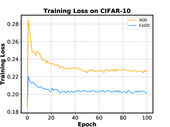
Figure 7: Comparison of training loss on CIFAR-10 with CoGD and SGD.

Synchronous convergence: In Fig. 7, the training curve shows that the convergence of CoGD is similar to that of GAL with SGD-based optimization within an epoch, especially for the last epochs when converging in a similar speed. We theoretically derive CoGD within the gradient descent framework, which provides a theoretical foundation for the convergence, which is validated by the experiments. As a summary, the main differences between SGD and CoGD are twofold. First, we change the initial point for each epoch. Second, we explore the coupling relationship between the hidden factors to improve a bilinear model within the gradient descent framework. Such differences do not change the convergence of CoGD compared with the SGD method.

In Fig. 8, we show the convergence in a synchronous manner of the $4$th layer’s variables when pruning CNNs. For better visualization, the learning rate of $\mathbf{m}$ is enlarged by 100$x$. On the curves, we observe that the two variables converge synchronously, and that neither variable gets stuck into a local minimum. This validates that CoGD avoids vanishing gradient for the coupled variables.

Table 5: Pruning results on CIFAR-10 with CoGD or SGD. M means million (${10^{6}}$).

Optimizer	Accuracy (%)	FLOPs / Baseline (M)
SGD	94.81	376.12 / 555.43
CoGD	95.30	274.74 / 555.43

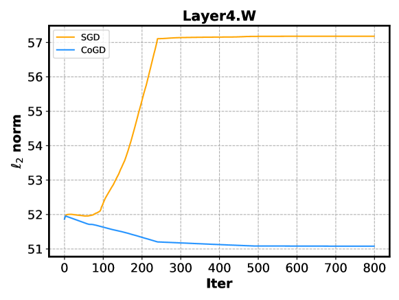
(a)

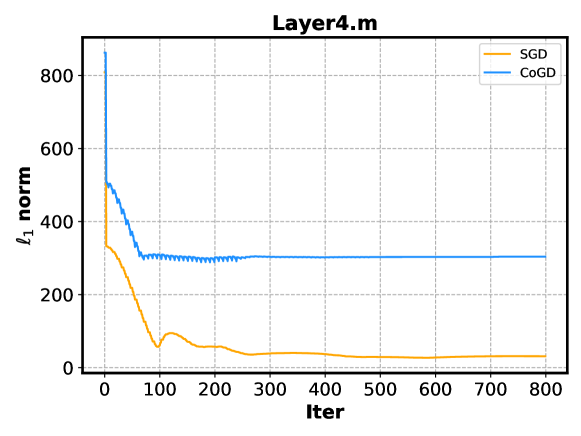
(b)

Figure 8: Convergence comparison of the variables in the 4th convolutional layer when pruning CNNs. The curves are obtained using SGD and CoGD-$0.5$ on CIFAR-10. With CoGD, the two variables converge synchronously while avoiding either variable gets stuck in a local convergence (local minimum of the objective function), which validates that CoGD can avoid vanishing gradient for the coupled variables.

5.4 CNN Training

Similar to network pruning, we have further evaluated CoGD algorithm for CNN model training on CIFAR-10 and ILSVRC12 ImageNet datasets. Specifically, we use ResNet-18 as the backbone CNN to test our algorithm. The network stages are 64-128-256-512. The learning rate is optimized by a cosine updating schedule with an initial learning rate $0.1$. The algorithm iterates $200$ epochs. The weight decay and momentum are respectively set to $0.0001$ and $0.9$. The model is trained on $2$ GPUs (Titan V) with a mini-batch size of $128$. We follow the similar augmentation strategy in He et al. (2016) and add the cutout method for training. When training the model, horizontal flipping and $32\times 32$ crop are used as data augmentation. The cutout size is set to $16$. Similar to CNNs pruning, $a$ is set to $0.95$ to compute $\alpha_{\gamma}$ and $\alpha_{W}$. To improve the efficiency, we directly backtrack the corresponding weights. For ILSVRC12 ImageNet, the initial learning rate is set to $0.01$, and the total epochs are $120$.

With ResNet-18 backbone, we simply replace the SGD algorithm with the proposed CoGD for model training. In Tab. 6, it can be seen that the performance is improved by $1.25$% (70.75% vs. 69.50%) on the large-scale ImageNet dataset. In addition, the improvement is also observed on CIFAR-10. We report the results for different kernels, which show that the performance are relatively stable for $k=1$ and $k=2$. These results validate the effectiveness and generality of the proposed CoGD algorithm.

Table 6: Results for CNN training on CIFAR-10 and ImageNet.

Models	Accuracy(%)
	CIFAR-10	ImageNet
ResNet-18 (SGD)He et al. (2016)	95.31	69.50
ResNet-18 (CoGD with K=1)	95.80	70.30
ResNet-18 (CoGD with K=2)	96.10	70.75

6 Conclusion

In this paper, we proposed a new learning algorithm, termed cogradient descent (CoGD), for the challenging yet important bilinear optimization problems with sparsity constraints. The proposed CoGD algorithm was applied on typical bilinear problems including convolutional sparse coding, network pruning, and CNN model training to solve important tasks including image reconstruction, image inpainting, and deep network optimization. Consistent and significant improvements demonstrated that CoGD outperforms previous gradient-based optimization algorithms. We further provided the solid derivation for CoGD, building an solid framework for leveraging a kernelized projection function to reveal the interaction of the variables in terms of convergence efficiency. Both the CoGD algorithm and the kernelized projection function provide a fresh insight to the fundamental gradient-based optimization problems.

Acknowledgments

We are thankful for the comments from Prof. Rongrong Ji for their deep and insightful discussion. We would also appreciate the editors and anonymous reviewers for their constructive comments.

References

- Abdelhamed et al. (2019) Abdelrahman Abdelhamed, Marcus A Brubaker, and Michael S Brown. Noise flow: Noise modeling with conditional normalizing flows. In ICCV, pages 3165–3173, 2019.
- Bau et al. (2017) David Bau, Bolei Zhou, Aditya Khosla, Aude Oliva, and Antonio Torralba. Network dissection: Quantifying interpretability of deep visual representations. In Computer Vision and Pattern Recognition, pages 3319–3327, 2017.
- Boyd et al. (2011) Stephen Boyd, Neal Parikh, Eric Chu, Borja Peleato, Jonathan Eckstein, et al. Distributed optimization and statistical learning via the alternating direction method of multipliers. Foundations and Trends® in Machine learning, 3(1):1–122, 2011.
- Bristow et al. (2013) Hilton Bristow, Anders Eriksson, and Simon Lucey. Fast convolutional sparse coding. In CVPR, pages 391–398, 2013.
- Choudhury et al. (2017) Biswarup Choudhury, Robin Swanson, Felix Heide, Gordon Wetzstein, and Wolfgang Heidrich. Consensus convolutional sparse coding. In ICCV, pages 4280–4288, 2017.
- Del Bue et al. (2011) Alessio Del Bue, Joao Xavier, Lourdes Agapito, and Marco Paladini. Bilinear modeling via augmented lagrange multipliers (balm). PAMI, 34(8):1496–1508, 2011.
- Denton et al. (2014) Emily Denton, Wojciech Zaremba, Joan Bruna, Yann Lecun, and Rob Fergus. Exploiting linear structure within convolutional networks for efficient evaluation. In NIPS, 2014.
- Ding et al. (2019) Xiaohan Ding, Guiguang Ding, Yuchen Guo, and Jungong Han. Centripetal sgd for pruning very deep convolutional networks with complicated structure. In CVPR, pages 4943–4953, 2019.
- Dozat (2016) Timothy Dozat. Incorporating nesterov momentum into adam. In International Conference on Learning Representations, pages 1–8, 2016.
- Goldt et al. (2019) Sebastian Goldt, Madhu S Advani, Andrew M Saxe, Florent Krzakala, and Lenka Zdeborová. Dynamics of stochastic gradient descent for two-layer neural networks in the teacher-student setup. arXiv preprint arXiv:1906.08632, 2019.
- Gu et al. (2015) Shuhang Gu, Wangmeng Zuo, Qi Xie, Deyu Meng, Xiangchu Feng, and Lei Zhang. Convolutional sparse coding for image super-resolution. In ICCV, pages 1823–1831, 2015.
- Guo et al. (2016) Yiwen Guo, Anbang Yao, and Yurong Chen. Dynamic network surgery for efficient dnns. In NIPS, pages 1379–1387, 2016.
- Han et al. (2015a) Song Han, Huizi Mao, and William J. Dally. Deep compression: Compressing deep neural networks with pruning, trained quantization and huffman coding. Fiber, 56(4):3–7, 2015a.
- Han et al. (2015b) Song Han, Jeff Pool, John Tran, and William Dally. Learning both weights and connections for efficient neural network. In NIPS, pages 1135–1143, 2015b.
- Hassibi and Stork (1993) Babak Hassibi and David G Stork. Second order derivatives for network pruning: Optimal brain surgeon. In NIPS, pages 164–171, 1993.
- He et al. (2016) Kaiming He, Xiangyu Zhang, Shaoqing Ren, and Jian Sun. Deep residual learning for image recognition. In CVPR, pages 770–778, 2016.
- He et al. (2019) Yang He, Ping Liu, Ziwei Wang, Zhilan Hu, and Yi Yang. Filter pruning via geometric median for deep convolutional neural networks acceleration. In CVPR, pages 4340–4349, 2019.
- He et al. (2017) Yihui He, Xiangyu Zhang, and Jian Sun. Channel pruning for accelerating very deep neural networks. In ICCV, pages 1398–1406, 2017.
- Heide et al. (2015) Felix Heide, Wolfgang Heidrich, and Gordon Wetzstein. Fast and flexible convolutional sparse coding. In CVPR, pages 5135–5143, 2015.
- Hinton et al. (2015) Geoffrey Hinton, Oriol Vinyals, and Jeff Dean. Distilling the knowledge in a neural network. Computer Science, 14(7):38–39, 2015.
- Hu et al. (2016) Hengyuan Hu, Rui Peng, Yu-Wing Tai, and Chi-Keung Tang. Network trimming: A data-driven neuron pruning approach towards efficient deep architectures. arXiv preprint arXiv:1607.03250, 2016.
- Huang et al. (2018) Gao Huang, Shichen Liu, Laurens Van der Maaten, and Kilian Q Weinberger. Condensenet: An efficient densenet using learned group convolutions. In CVPR, pages 2752–2761, 2018.
- Huang and Wang (2018a) Zehao Huang and Naiyan Wang. Data-driven sparse structure selection for deep neural networks. In ECCV, pages 304–320, 2018a.
- Huang and Wang (2018b) Zehao Huang and Naiyan Wang. Data-driven sparse structure selection for deep neural networks. In ECCV, pages 304–320, 2018b.
- Kingma and Ba (2014) Diederik P. Kingma and Jimmy Ba. Adam: A method for stochastic optimization. Computer Science, 2014.
- Krizhevsky et al. (2012) Alex Krizhevsky, Ilya Sutskever, and Geoffrey E Hinton. Imagenet classification with deep convolutional neural networks. In NIPS, pages 1097–1105, 2012.
- Krogh and Hertz (1992) Anders Krogh and John A Hertz. A simple weight decay can improve generalization. In NIPS, pages 950–957, 1992.
- LeCun et al. (1990) Yann LeCun, John S Denker, and Sara A Solla. Optimal brain damage. In NIPS, pages 598–605, 1990.
- Lemaire et al. (2019) Carl Lemaire, Andrew Achkar, and Pierre-Marc Jodoin. Structured pruning of neural networks with budget-aware regularization. In CVPR, pages 9108–9116, 2019.
- Li et al. (2016) Hao Li, Asim Kadav, Igor Durdanovic, Hanan Samet, and Hans Peter Graf. Pruning filters for efficient convnets. arXiv preprint arXiv:1608.08710, 2016.
- Li et al. (2017) Yanghao Li, Naiyan Wang, Jiaying Liu, and Xiaodi Hou. Factorized bilinear models for image recognition. In ICCV, pages 2079–2087, 2017.
- Li et al. (2019) Yuchao Li, Shaohui Lin, Baochang Zhang, Jianzhuang Liu, David Doermann, Yongjian Wu, Feiyue Huang, and Rongrong Ji. Exploiting kernel sparsity and entropy for interpretable cnn compression. In CVPR, pages 2800–2809, 2019.
- Liao et al. (2019) Qiyu Liao, Dadong Wang, Hamish Holewa, and Min Xu. Squeezed bilinear pooling for fine-grained visual categorization. In ICCV Workshop, October 2019.
- Lin et al. (2020) Mingbao Lin, Rongrong Ji, Yan Wang, Yichen Zhang, Baochang Zhang, Yonghong Tian, and Shao Ling. Hrank: Filter pruning using high-rank feature map. In IEEE Conference on Computer Vision and Pattern Recognition (CVPR), 2020.
- Lin et al. (2018) Shaohui Lin, Rongrong Ji, Yuchao Li, Yongjian Wu, Feiyue Huang, and Baochang Zhang. Accelerating convolutional networks via global & dynamic filter pruning. In IJCAI, pages 2425–2432, 2018.
- Lin et al. (2019) Shaohui Lin, Rongrong Ji, Chenqian Yan, Baochang Zhang, and David Doermann. Towards optimal structured cnn pruning via generative adversarial learning. In CVPR, 2019.
- Lin et al. (2015) Tsung-Yu Lin, Aruni RoyChowdhury, and Subhransu Maji. Bilinear cnn models for fine-grained visual recognition. In ICCV, pages 1449–1457, 2015.
- Liu et al. (2017) Zhuang Liu, Jianguo Li, Zhiqiang Shen, Gao Huang, Shoumeng Yan, and Changshui Zhang. Learning efficient convolutional networks through network slimming. In ICCV, pages 2736–2744, 2017.
- Luo et al. (2017) Jianhao Luo, Jianxin Wu, and Weiyao Lin. Thinet: A filter level pruning method for deep neural network compression. In ICCV, pages 5068–5076, 2017.
- Mairal et al. (2010) Julien Mairal, Francis Bach, Jean Ponce, and Guillermo Sapiro. Online learning for matrix factorization and sparse coding. Journal of Machine Learning Research, 11(Jan):19–60, 2010.
- Molchanov et al. (2016) Pavlo Molchanov, Stephen Tyree, Tero Karras, Timo Aila, and Jan Kautz. Pruning convolutional neural networks for resource efficient inference. arXiv preprint arXiv:1611.06440, 2016.
- Parikh et al. (2014) Neal Parikh, Stephen Boyd, et al. Proximal algorithms. Foundations and Trends® in Optimization, 1(3):127–239, 2014.
- Paszke et al. (2019) Adam Paszke, Sam Gross, Francisco Massa, Adam Lerer, James Bradbury, Gregory Chanan, Trevor Killeen, Zeming Lin, Natalia Gimelshein, Luca Antiga, et al. Pytorch: An imperative style, high-performance deep learning library. In Advances in Neural Information Processing Systems, pages 8024–8035, 2019.
- Petersen et al. (2008) Kaare Brandt Petersen, Michael Syskind Pedersen, et al. The matrix cookbook. Technical University of Denmark, 7(15):510, 2008.
- Rastegari et al. (2016) Mohammad Rastegari, Vicente Ordonez, Joseph Redmon, and Ali Farhadi. Xnor-net: Imagenet classification using binary convolutional neural networks. In ECCV, 2016.
- Romero et al. (2015) Adriana Romero, Nicolas Ballas, Samira Ebrahimi Kahou, Antoine Chassang, and Yoshua Bengio. Fitnets: Hints for thin deep nets. Computer Science, 2015.
- Sandler et al. (2018) Mark Sandler, Andrew Howard, Menglong Zhu, Andrey Zhmoginov, and Liang-Chieh Chen. Mobilenetv2: Inverted residuals and linear bottlenecks. In CVPR, pages 4510–4520, 2018.
- Sch et al. (2004) Christian Sch, Ivan Laptev, and Barbara Caputo. Recognizing human actions: A local svm approach. In ICPR, 2004.
- Suh et al. (2018) Yumin Suh, Jingdong Wang, Siyu Tang, Tao Mei, and Kyoung Mu Lee. Part-aligned bilinear representations for person re-identification. In ECCV, pages 402–419, 2018.
- Wohlberg (2014) Brendt Wohlberg. Efficient convolutional sparse coding. In ICASSP, pages 7173–7177, 2014.
- Wu et al. (2016) Jiaxiang Wu, Leng Cong, Yuhang Wang, Qinghao Hu, and Cheng Jian. Quantized convolutional neural networks for mobile devices. In CVPR, 2016.
- Yang et al. (2017a) Linlin Yang, Ce Li, Jungong Han, Chen Chen, Qixiang Ye, Baochang Zhang, Xianbin Cao, and Wanquan Liu. Image reconstruction via manifold constrained convolutional sparse coding for image sets. JSTSP, 11(7):1072–1081, 2017a.
- Yang et al. (2017b) Tien-Ju Yang, Yu-Hsin Chen, and Vivienne Sze. Designing energy-efficient convolutional neural networks using energy-aware pruning. In CVPR, pages 5687–5695, 2017b.
- Ye et al. (2018) Jianbo Ye, Xin Lu, Zhe Lin, and James Z Wang. Rethinking the smaller-norm-less-informative assumption in channel pruning of convolution layers. In ICLR, 2018.
- Yokoya et al. (2012) Naoto Yokoya, Jocelyn Chanussot, and Akira Iwasaki. Generalized bilinear model based nonlinear unmixing using semi-nonnegative matrix factorization. In IEEE International Geoscience and Remote Sensing Symposium, pages 1365–1368, 2012.
- Yoon and Hwang (2017) Jaehong Yoon and Sung Ju Hwang. Combined group and exclusive sparsity for deep neural networks. In ICML, pages 3958–3966. JMLR. org, 2017.
- Young et al. (2019) Sean I. Young, Aous T. Naman, Bernd Girod, and David Taubman. Solving vision problems via filtering. In ICCV, October 2019.
- Yu et al. (2018) Ruichi Yu, Ang Li, Chun-Fu Chen, Jui-Hsin Lai, Vlad I Morariu, Xintong Han, Mingfei Gao, Ching-Yung Lin, and Larry S Davis. Nisp: Pruning networks using neuron importance score propagation. In CVPR, page 9194–9203, 2018.
- Yu et al. (2017) Zhou Yu, Jun Yu, Jianping Fan, and Dacheng Tao. Multi-modal factorized bilinear pooling with co-attention learning for visual question answering. In ICCV, pages 1821–1830, 2017.
- Zagoruyko and Komodakis (2016) Sergey Zagoruyko and Nikos Komodakis. Paying more attention to attention: Improving the performance of convolutional neural networks via attention transfer. 2016.
- Zeiler (2012) Matthew D Zeiler. Adadelta: An adaptive learning rate method. arXiv preprint, 2012.
- Zeiler et al. (2010) Matthew D Zeiler, Dilip Krishnan, Graham W Taylor, and Rob Fergus. Deconvolutional networks. In CVPR, pages 2528–2535. IEEE, 2010.
- Zhang et al. (2015) Baochang Zhang, Alessandro Perina, Vittorio Murino, and Alessio Del Bue. Sparse representation classification with manifold constraints transfer. In CVPR, June 2015.
- Zhang et al. (2012) Lei Zhang, Meng Yang, Xiangchu Feng, Yi Ma, and David Zhang. Collaborative representation based classification for face recognition. arXiv preprint arXiv:1204.2358, 2012.
- Zhang K (2018) et al. Zhang K, Schölkopf B. Learning causality and causality-related learning: some recent progress. National science review, 2018.
- Zhou et al. (2019) Yuefu Zhou, Ya Zhang, Yanfeng Wang, and Qi Tian. Accelerate cnn via recursive bayesian pruning. In ICCV, pages 3306–3315, 2019.
- Zhuo et al. (2020) Li’an Zhuo, Baochang Zhang, Linlin Yang, Hanlin Chen, Qixiang Ye, David S. Doermann, Guodong Guo, and Rongrong Ji. Cogradient descent for bilinear optimization. CoRR, abs/2006.09142, 2020.