The XMM-SERVS survey: XMM-Newton point-source catalogs for the W-CDF-S and ELAIS-S1 fields

Abstract

We present the X-ray point-source catalogs in two of the XMM-Spitzer Extragalactic Representative Volume Survey (XMM-SERVS) fields, W-CDF-S (4.6 deg²) and ELAIS-S1 (3.2 deg²), aiming to fill the gap between deep pencil-beam X-ray surveys and shallow X-ray surveys over large areas. The W-CDF-S and ELAIS-S1 regions were targeted with 2.3 Ms and 1.0 Ms of XMM-Newton observations, respectively; 1.8 Ms and 0.9 Ms exposures remain after flare filtering. The survey in W-CDF-S has a flux limit of $1.0\times 10^{-14}$ erg cm^-2 s^-1 over 90% of its area in the 0.5–10 keV band; 4053 sources are detected in total. The survey in ELAIS-S1 has a flux limit of $1.3\times 10^{-14}$ erg cm^-2 s^-1 over 90% of its area in the 0.5–10 keV band; 2630 sources are detected in total. Reliable optical-to-IR multiwavelength counterpart candidates are identified for $\approx$ 89% of the sources in W-CDF-S and $\approx$ 87% of the sources in ELAIS-S1. 3186 sources in W-CDF-S and 1985 sources in ELAIS-S1 are classified as AGNs. We also provide photometric redshifts for X-ray sources; $\approx$ 84% of the 3319/2001 sources in W-CDF-S/ELAIS-S1 with optical-to-NIR forced photometry available have either spectroscopic redshifts or high-quality photometric redshifts. The completion of the XMM-Newton observations in the W-CDF-S and ELAIS-S1 fields marks the end of the XMM-SERVS survey data gathering. The $\approx$ 12,000 point-like X-ray sources detected in the whole $\approx 13$ deg² XMM-SERVS survey will benefit future large-sample AGN studies.

1 Introduction

Owing to the penetrating nature of X-rays and their reduced dilution by host-galaxy starlight, X-ray surveys have been effectively utilized to identify reliable and nearly complete samples of active galactic nuclei (AGNs), which provide essential insights into the demographics, ecology, and physics of growing supermassive black holes (SMBHs) over most of cosmic history (e.g., Brandt & Alexander, 2015; Xue, 2017).

XMM-Newton and Chandra surveys have provided the most efficient method in assembling reliable and quite complete samples of distant AGNs, including obscured systems otherwise difficult to find. The currently publicly available wide-field X-ray surveys such as the 8–10 ks XMM-Newton depth Stripe 82X (LaMassa et al., 2016) and XMM-XXL (e.g., Liu et al., 2016) have made excellent progress sampling the luminous AGN populations and their environments. At the same time, they lack the sensitivity to detect the bulk of SMBH growth as they only probe $\approx 2$–6 times below the knee of the X-ray luminosity function at $z=0.5$–2.5, and the AGNs detected produce less than half of cosmic accretion power (e.g., Ueda et al., 2014; Aird et al., 2015). The narrow-field deep X-ray surveys (0.1–1.1 deg²), such as the CDF-S (Luo et al., 2017), CDF-N (Xue et al., 2016), E-CDF-S (Xue et al., 2016), AEGIS-X (Nandra et al., 2015), and SXDS (Ueda et al., 2008), are able to sample AGNs that produce the bulk ($>$ 70%) of cosmic accretion power at $z\lesssim 3$–5 well (e.g., Ueda et al., 2014; Aird et al., 2015; Vito et al., 2018). However, they do not have the contiguous volume needed to explore AGN activity over a wide dynamic range of cosmic environments and to sample substantially the high-luminosity tail of the AGN population. Simulations indicate that at $z\approx 1$, the largest structures (e.g., superclusters) extend up to 2–3 deg² on the sky (e.g., Klypin et al. 2016). Thus, even the $\approx 2$ deg² COSMOS field (e.g., Cappelluti et al., 2009; Civano et al., 2016) is not able to sample the full range of cosmic environments. Therefore, it is necessary to obtain several distinct medium-deep X-ray surveys, each over several deg², in addition to COSMOS for investigating SMBH growth across the full range of cosmic environments and minimizing cosmic variance (e.g., Driver & Robotham, 2010; Moster et al., 2011).

To this end, we designed an XMM-Newton survey, XMM-SERVS, to provide medium-deep X-ray coverage in the SERVS (Mauduit et al., 2012) regions of the W-CDF-S ($\approx$ 4.6 deg²), ELAIS-S1 ($\approx$ 3.2 deg²), and XMM-LSS ($\approx$ 5.3 deg²) fields, all of which have superb multiwavelength coverage. The point-source catalog for the XMM-LSS field has been published in Chen et al. (2018). In this work, we provide point-source catalogs for the two remaining fields, W-CDF-S and ELAIS-S1. Data products from the full XMM-SERVS survey (including all the three fields) are available online.

The paper is structured as follows. Section 2 describes the new XMM-Newton observations in the W-CDF-S and ELAIS-S1 fields as well as overlapping archival multiwavelength data in these areas. Section 3 presents the X-ray source detection process and the properties of the derived X-ray sources. Section 4 describes the multiwavelength counterpart identification process for the X-ray sources. Section 5 presents spectroscopic redshifts and photometric redshifts of X-ray sources. In Section 6, basic AGN classification is presented. Section 7 gives the summary of the work. Appendix A describes the columns included in our X-ray source catalogs. Appendix B describes the identification of broad-line (BL) AGNs among the X-ray sources detected. Appendix C describes the classification of X-ray sources that are not AGNs. A $\Lambda$CDM cosmology with $H_{0}=70$ km s^-1 Mpc^-1, $\Omega_{m}=0.3$, and $\Omega_{\Lambda}=0.7$ is assumed throughout the paper. A Galactic column density $N_{\rm H}=8.4\times 10^{19}~{}\rm cm^{-2}$ is adopted for the W-CDF-S field, and $N_{\rm H}=3.4\times 10^{20}~{}\rm cm^{-2}$ is adopted for the ELAIS-S1 field (Willingale et al., 2013).

2 XMM-Newton observations in the W-CDF-S and ELAIS-S1 regions

2.1 Multiwavelength data coverage and archival XMM-Newton and Chandra observations in the W-CDF-S region

There are deep archival Chandra and XMM-Newton observations in the center of the $\approx 4.5$ deg² W-CDF-S field, covering a relatively small area (see Figure 1). The Chandra Deep Field-South (CDF-S) survey has now reached a 7 Ms depth, covering 482 arcmin² (e.g., Xue et al., 2011; Luo et al., 2017); XMM-Newton has also observed this field for 3.3 Ms (covering $\approx$ 790 arcmin²; e.g., Comastri et al. 2011; Ranalli et al. 2013). The 250 ks Extended Chandra Deep Field-South (E-CDF-S) survey further increases the X-ray coverage to 1128.6 arcmin² (e.g., Xue et al., 2016). There are also several additional $\approx 5$–15 ks Chandra observations in the W-CDF-S region (including four observations just to the south of E-CDF-S; PI: W. N. Brandt). These Chandra data are utilized in our study to help the multiwavelength counterpart matching of XMM-Newton sources (see Section 4). All of the above X-ray observations along with the multiwavelength data have enabled many AGN studies.

The W-CDF-S region, which is $\approx 30$ times larger in solid angle than the original CDF-S, also has extensive multiwavelength coverage (see Table 1 for a list of the key multiwavelength photometric data). It aligns with one of the well-studied Spitzer Extragalactic Representative Volume Survey (SERVS; Mauduit et al. 2012) fields, and it is also one of the deep-drilling fields of the upcoming Legacy Survey of Space and Time (LSST) to be conducted by the Vera C. Rubin Observatory (e.g., Brandt et al., 2018; Scolnic et al., 2018). With the XMM-SERVS survey covering the W-CDF-S region, multiwavelength data in this area can be utilized together with the X-ray data, enabling large-sample studies of AGNs and other X-ray sources.

Table 1: Key multiwavelength imaging coverage of the W-CDF-S and ELAIS-S1 fields.

Band	Field(s)∗	Survey Name	Coverage; Notes	Example Reference
Radio	C/E	Australia Telescope Large Area Survey (ATLAS)	3.6/2.7 deg2; 14/17 $\mu$Jy rms depth at 1.4 GHz	Franzen et al. (2015)
	C/E	MIGHTEE Survey (in progress)	3/4.5 deg2; 1 $\mu$Jy rms depth at 1.4 GHz	Jarvis et al. (2016)
MIR–FIR	C/E	Herschel Multi-tiered Extragal. Surv. (HerMES)	11.4/3.7 deg2; 5–60 mJy depth at 100–500 $\mu$m	Oliver et al. (2012)
	C/E	Spitzer Wide-area IR Extragal. Survey (SWIRE)	7.1/14.3 deg2; 0.01–200 mJy depth at 3.6–160 $\mu$m	Vaccari (2015)
NIR	C/E	Spitzer survey of Deep Drilling Fields (DeepDrill)	9/9 deg2; 2 $\mu$Jy depth at 3.6 and 4.5 $\mu$m	Lacy et al. (2021)
	C/E	Spitzer Extragal. Rep. Vol. Survey (SERVS)	4.5/3 deg2; 2 $\mu$Jy depth at 3.6 and 4.5 $\mu$m	Mauduit et al. (2012)
	C/E	VISTA Deep Extragal. Obs. Survey (VIDEO)	4.5/3 deg2; $ZYJHK_{s}$ to $m_{\rm AB}\approx 23.8$–25.7	Jarvis et al. (2013)
Optical	C/E	Dark Energy Survey (DES) Data Release 2	9/6 deg2; $grizy$ to $m_{\rm AB}\approx 23$–25.5	Abbott et al. (2021)
	C	Hyper Suprime Cam (HSC) optical imaging	5.7 deg2; $griz$ to $m_{\rm AB}\approx 25$–26	Ni et al. (2019)
	C	VST Opt. Imaging of CDF-S and ES1 (VOICE)	4 deg2; $ugri$ to $m_{\rm AB}\approx 26$	Vaccari et al. (2016)
	E	VST Opt. Imaging of CDF-S and ES1 (VOICE)	4 deg2; $u$ to $m_{\rm AB}\approx 26$, $gri$ observations planned	Vaccari et al. (2016)
	C	SWIRE optical imaging	7.1 deg2; $u^{\prime}g^{\prime}r^{\prime}i^{\prime}z^{\prime}$ to $m_{\rm AB}\approx 23$–25	Lonsdale et al. (2003)
	E	ESO-Spitzer Imaging Extragalactic Survey (ESIS)	4.5 deg2; $BVR$ to $m_{\rm AB}\approx 24$–25	Berta et al. (2006)
	C/E	LSST deep-drilling field (Planned)	10/10 deg2; $ugrizy$ to $m_{\rm AB}\approx 26$–28	Brandt et al. (2018)
UV	C/E	GALEX Deep Imaging Survey	7/15 deg2; NUV, FUV to $m_{\rm AB}\approx 24$–24.5	Martin et al. (2005)

^∗“C” stands for W-CDF-S; “E” stands for ELAIS-S1.

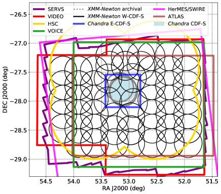
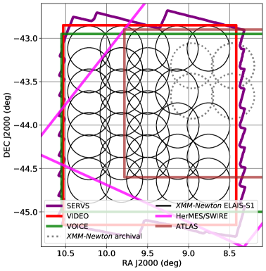
Figure 1: Left: Locations of the XMM-Newton observations in the W-CDF-S field (black circles), presented together with the multiwavelength coverage from selected surveys and the primary archival X-ray observations in this area (as labeled in the figure key). DES wide-field survey (see Table 1) in the optical cover the whole area, and thus are not plotted in the figure. Right: Locations of the XMM-Newton observations in the ELAIS-S1 field (black circles), presented together with the selected multiwavelength coverage and the primary archival X-ray observations in this area (as labeled in the figure key). DES wide-field survey and ESIS (see Table 1) in the optical cover the whole area, and thus are not plotted in the figure.

2.2 Multiwavelength data coverage and archival XMM-Newton and Chandra observations in the ELAIS-S1 region

About 0.6 deg² of the $\approx 3$ deg² ELAIS-S1 region has been targeted with both XMM-Newton ($\approx 50$ ks depth) and Chandra ($\approx 30$ ks depth) (e.g., Puccetti et al., 2006; Feruglio et al., 2008). There are also several additional Chandra observations in the ELAIS-S1 region. The multiwavelength data coverage of the ELAIS-S1 field is listed in Table 1. Similar to the W-CDF-S field, ELAIS-S1 aligns with one of the SERVS fields, and will be one of the LSST deep-drilling fields. As can be seen in Table 1, the optical data in ELAIS-S1 are not yet as deep as that in W-CDF-S (also see Zou et al. 2021 for further details).

2.3 New XMM-Newton observations and data reduction

XMM-Newton observations in the W-CDF-S field were obtained between July 2018 to January 2021 (see the left panel of Figure 1 for the pointing layout) with a total of 2.3 Ms exposure time, including 80 successful observations. For the ELAIS-S1 field, XMM-Newton observations were performed between May 2019 to December 2020 (see the right panel of Figure 1 for the pointing layout), with a total of 1.0 Ms exposure time, including 31 successful observations. All the observations were performed with a THIN filter for the EPIC cameras, and Optical Monitor data were taken in parallel as well (we do not include these data in our catalogs, due to the exisiting optical/UV coverage listed in Table 1). As these fields are far from the Galactic plane, the numbers of very bright stars in these fields are small, and the optical loading effects for the X-ray CCDs are negligible. The details of each observation are listed in Table 2. As described in Chen et al. (2018), we first observed the desired pointings with 33 ks exposures, and then re-observed the sky regions strongly affected by XMM-Newton background flaring to achieve better uniformity. For the W-CDF-S field, we do not re-analyze all of the archival XMM-Newton observations of the CDF-S proper (that cover $\approx 0.25$ deg²) in this work; instead, we selected one observation (ObsID: 0604960501) from the archival data to reach a uniform depth across the W-CDF-S field and process this consistently in the same manner as the rest of our data. For the ELAIS-S1 field, all the archival XMM-Newton observations are included in the analyses.

Table 2: XMM-Newton observations in the W-CDF-S and ELAIS-S1 fields. This table is available in its entirety online.

Field	Revolution	ObsID	UT Date	R.A.	Decl.	GTI (PN)	GTI (MOS1)	GTI (MOS2)	Expo
				(deg)	(deg)	(ks)	(ks)	(ks)	(ks)
W-CDF-S	3403	0827210101	2018-07-08 23:34:26	52.579042	$-$28.723972	27.9	30.5	29.7	33
W-CDF-S	3403	0827210201	2018-07-09 09:04:26	52.582875	$-$28.473972	27.9	29.4	29.2	33
W-CDF-S	3406	0827210301	2018-07-15 05:20:04	52.586667	$-$28.223972	28.9	30.7	30.6	33
ELAIS-S1	3561	0827251301	2019-05-20 07:26:00	9.143708	$-$43.614139	28.8	30.5	30.6	33
ELAIS-S1	3568	0827240101	2019-06-03 05:48:52	8.757958	$-$44.004000	29.4	31.6	31.3	34

Columns from left to right: target field, XMM-Newton revolution, XMM-Newton Observation ID, observation starting date/time, Right Ascension and Declination of the pointing center (J2000, degrees), cleaned exposure time (included in the “good time intervals”; GTIs) for PN, MOS1, and MOS2 in each pointing, total EPIC exposure time (during which PN, MOS1, and MOS2 take exposures simultaneously).

The XMM-Newton Science Analysis System (SAS) 19.0.0 and HEASOFT 6.26 are utilized for our data analysis. We use the SAS tasks epproc and emproc to process the XMM-Newton Observation Data Files (ODFs), creating MOS1, MOS2, PN, and PN out-of-time (OOT) event files for each observation ID. Following Section 2.2 of Chen et al. (2018), single-event light curves are created for each event file in time bins of 100 s at high (10–12 keV) and low (0.3–10 keV) energies to select time intervals without significant background flares (the “good time intervals”; GTIs); we note that real sources provide minimal contributions to these total event file light curves. For the 10–12 keV light curve, we remove time intervals with count rates $>3\sigma$ above the mean count rate. The same procedure is also performed for the 0.3–10 keV light curves. For a small number of event files with intense background flares, the event files are filtered using the nominal count-rate thresholds suggested by the XMM-Newton Science Operations Centre.

For the W-CDF-S field, a total of 1.8 Ms (1.5 Ms) of MOS (PN) exposure remains after flare filtering; for the ELAIS-S1 field, a total of 0.9 Ms (0.8 Ms) of MOS (PN) exposure remains. We do not exclude events in energy ranges that overlap with the instrumental background lines (Al K$\alpha$ lines at 1.39–1.55 keV for MOS and PN; Cu lines at 7.35–7.60 keV and 7.84–8.28 keV for PN; Si lines at 1.69–1.80 keV for MOS), as keeping these events improves the positional accuracy of the detected sources due to the higher number of counts detected.

We use evselect to construct images with a $4^{\prime\prime}$ pixel size from the flare-filtered event file in the full band (0.2–12 keV). We use eexpmap to generate exposure maps with usefastpixelization=0 and attrebin=0.5, both with and without vignetting corrections. Detector masks were constructed with emask. The mosaicked vignetting-corrected PN+MOS1+MOS2 exposure map in the W-CDF-S/ELAIS-S1 field and the distribution of the exposure time across the survey field are presented in Figures 2 and 3. As can be seen in Figure 3, $\approx$ 4.6 deg² of the W-CDF-S field is covered by XMM-Newton; $\approx$ 3.2 deg² of the ELAIS-S1 field is covered by XMM-Newton. The median PN+MOS1+MOS2 exposure time across the W-CDF-S/ELAIS-S1 field is $\approx$ 84/80 ks. More than 80% of the W-CDF-S/ELAIS-S1 footprints have PN+MOS1+MOS2 exposure time $\gtrsim$ 47/37 ks. Figure 3 shows the cumulative survey solid angle as a function of full-band effective exposure for the full three-field XMM-SERVS survey. The median PN+MOS1+MOS2 exposure time across the full XMM-SERVS survey field is $\approx$ 85 ks.

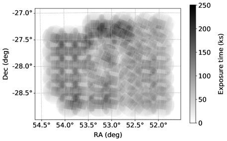
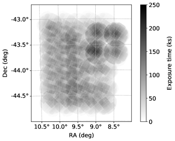
Figure 2: Left: Effective exposure map (PN + MOS) in the full band for W-CDF-S. The XMM-Newton coverage in the survey region is generally uniform. Right: Similar to the left panel, but for ELAIS-S1.

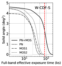
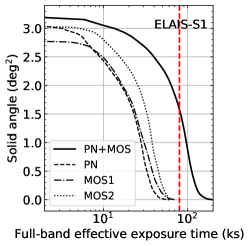
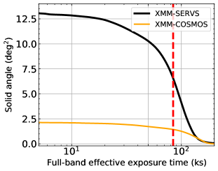
Figure 3: Cumulative survey solid angle as a function of full-band effective (i.e., vignetted) exposure in W-CDF-S (Left), ELAIS-S1 (middle), and the entire XMM-SERVS survey (right). The black solid/dashed/dash-dotted/dotted line is for the PN+MOS/PN/MOS1/MOS2 exposure. The relatively small solid angle of MOS1 coverage is due to the lost CCDs for MOS1. The solid orange line in the right panel is for the PN+MOS exposure in XMM-COSMOS (Cappelluti et al., 2009). The red vertical line marks the median exposure.

3 Source detection and the main X-ray source catalogs

3.1 First-pass source detection and astrometric correction

Following Chen et al. (2018), we run a first-pass source detection in the full band to register the XMM-Newton observations onto a common World Coordinate System (WCS) frame with the following steps:

1. For each observation, eboxdetect is used to generate a temporary source list with likemin=8 for each of the three instruments.

2. This temporary source list is utilized to generate background images for each instrument (with the input sources removed), using esplinemap with method=asmooth. This adaptive-smoothing method has been widely adopted in recent XMM-Newton catalogs (e.g., Traulsen et al., 2019, 2020; Webb et al., 2020), as it can well-characterize the local X-ray background level.

3. We run eboxdetect again in the map mode (with likemin=8), combining images, exposure maps, and background maps from all the instruments for each observation.

4. With this new source list generated by eboxdetect as the input, the PSF-fitting tool emldetect is used to determine the X-ray positions and detection likelihoods utilizing all the instruments of each observation. We only keep the point-like sources, and a stringent likelihood threshold (likemin $=10.8$) is adopted to ensure that astrometric corrections are calculated based on significant detections that are unlikely to be spurious.

For each observation, we use catcorr to match the output source list from emldetect with an optical/IR reference catalog (available from the relevant XMM-Newton Processing Pipeline Subsystem products; Rosen et al. 2016) created from the Sloan Digital Sky Survey (SDSS; Abazajian et al. 2009), 2MASS (Skrutskie et al., 2006), and USNO-B1.0 (Monet et al., 2003) catalogs. By matching the X-ray sources to the reference catalogs (the median number of matched sources is 18 among all the observations), the needed astrometric offsets and rotation corrections are calculated. The RA/DEC offsets are typically $\lesssim 3^{\prime\prime}$. The rotation corrections are less than $\approx 0.17$ deg. The event files and the attitude file for each observation are then projected onto the new frame.

3.2 Second-pass source detection

Using the astrometry-corrected event files, we re-create images (see Figure 4 for the smoothed full-field mosaicked XMM-Newton images for W-CDF-S and ELAIS-S1, and Figure 5 for an example cutout of the smoothed mosaicked image in W-CDF-S), exposure maps, detector masks, and background maps in five bands: band 1 (0.2–0.5 keV), band 2 (0.5–1.0 keV), band 3 (1.0–2.0 keV), band 4 (2.0–4.5 keV), and band 5 (4.5–12 keV). We define the full band as bands 1–5 (0.2–12 keV), soft band as bands 1–3 (0.2–2 keV), and hard band as bands 4–5 (2–12 keV). Exposure maps and image mosaics are also created for the full/soft/hard band combining all the observations and instruments in the full/soft/hard band. We then run source detection again with data products from bands 1, 2, 3, 4, and 5, combining all XMM-Newton observations together. This five-band detection approach has been widely adopted in XMM-Newton catalogs (e.g., Rosen et al., 2016; Traulsen et al., 2019, 2020; Webb et al., 2020) since it improves the positional accuracy of sources detected compared to single-band detections. When detecting sources in the full band (0.2–12 keV), we use bands 1–5 simultaneously; when detecting sources in the soft band (0.2–2 keV), we use bands 1–3 simultaneously; when detecting sources in the hard band (2–12 keV), we use bands 4–5 simultaneously. As emldetect can only process a limited number of observations, we divide the W-CDF-S/ELAIS-S1 field into a grid when performing the second-pass source detection (e.g., Chen et al., 2018). For each cell in the grid, we coadd the images and exposure maps for all observations inside the cell, and run ewavelet with a low detection threshold (4) in the full/soft/hard band. The source list obtained from ewavelet is then utilized as the input for emldetect (only sources within the celestial coordinate range of the cell plus 1 arcmin “padding” on each side of the cell are kept). The full/soft/hard-band source list from emldetect in each cell is then combined to remove duplications (sources in the “padding” area that do not have duplications within 10^′′ are kept). For each band in each field, we select sources with detection likelihoods (det_ml) larger than the threshold that corresponds to a 1% spurious fraction according to simulations (see Section 3.3 for details).

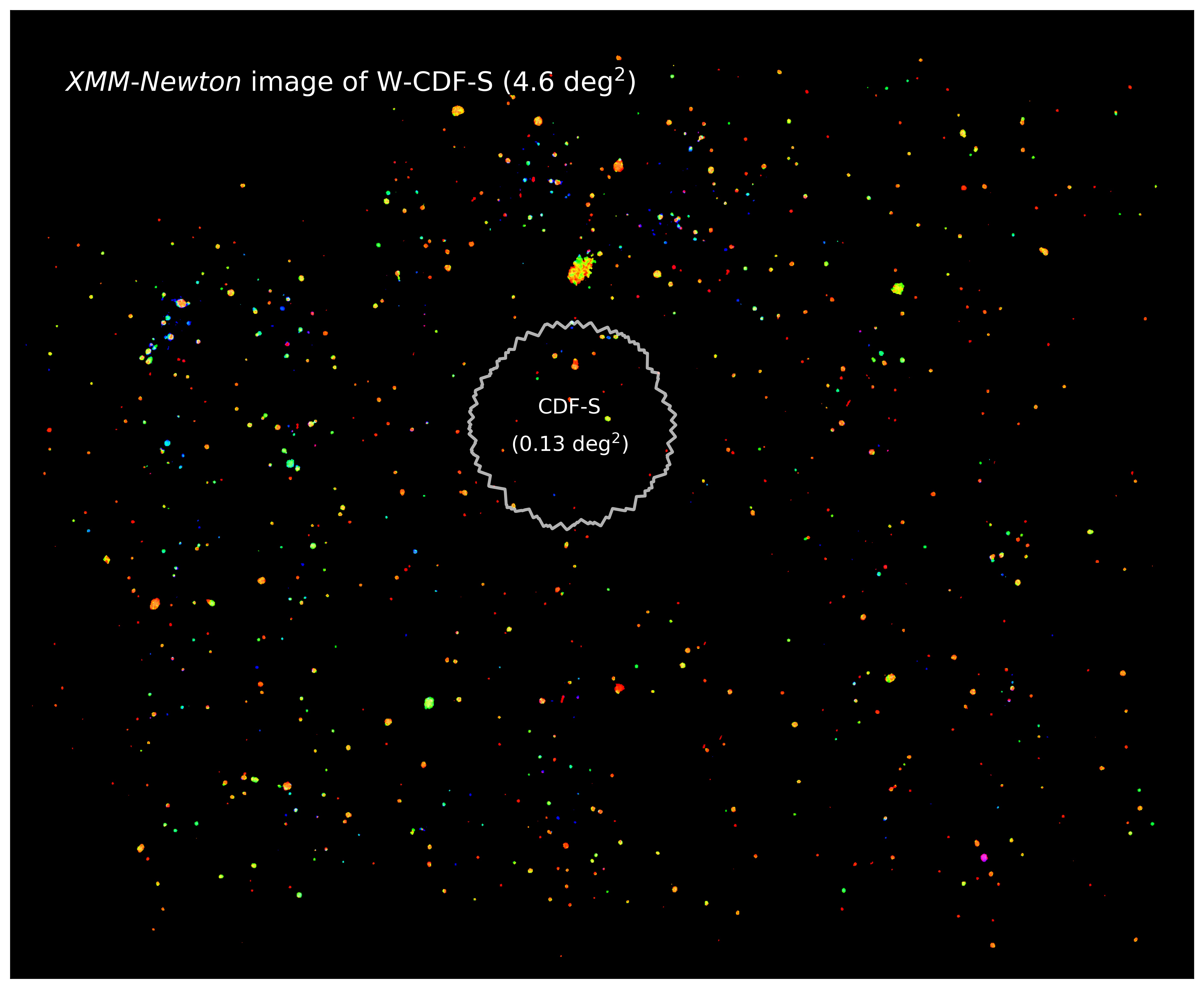
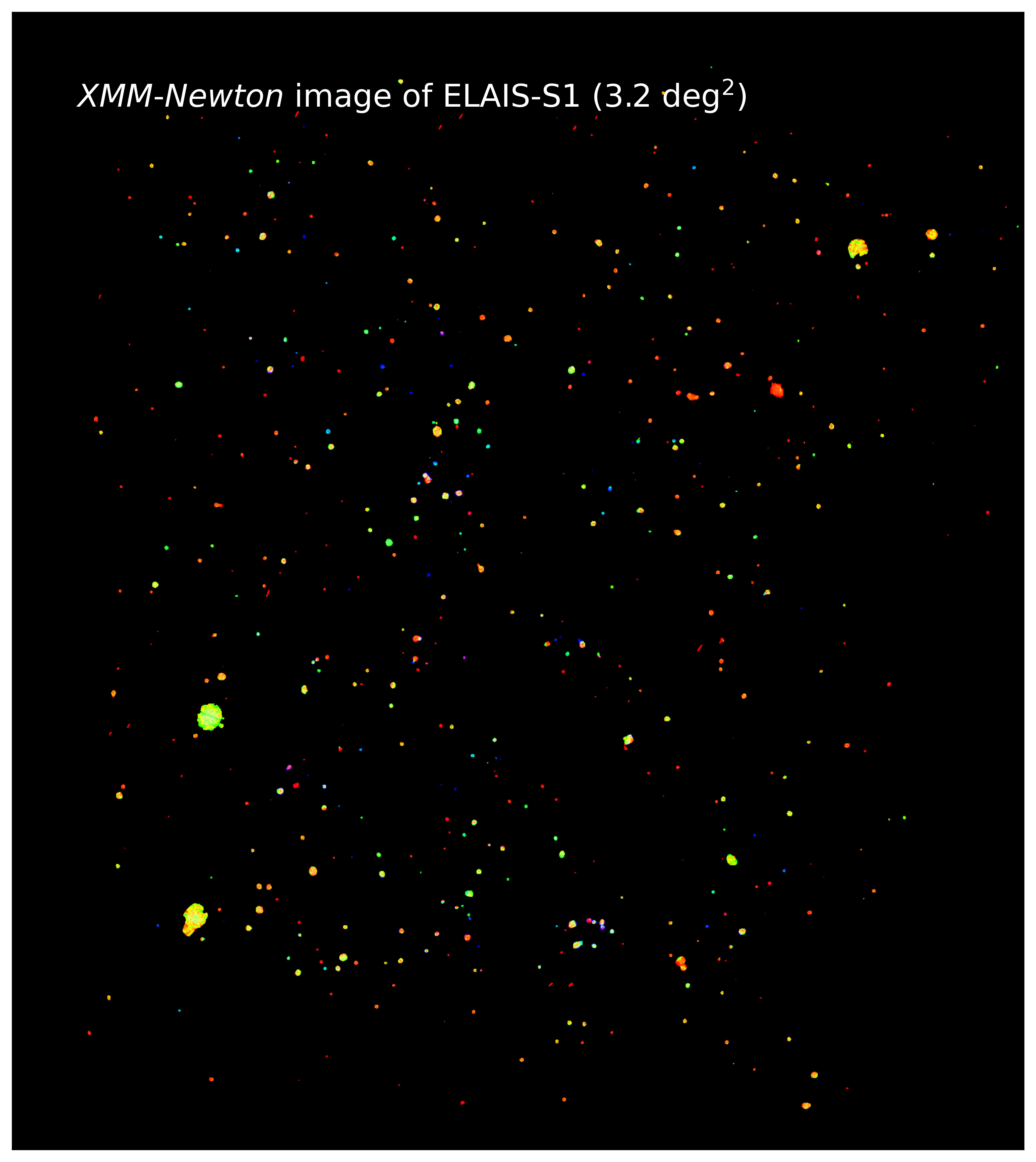
Figure 4: Left: “False-color” smoothed X-ray image of W-CDF-S. Band 1+2, band 3, and band 4+5 are represented by the colors red, green, and blue, respectively. Redder sources are softer; bluer sources are harder. An asinh stretch is utilized. The white solid curve indicates the footprint of the 7 Ms CDF-S (Luo et al., 2017). Right: Similar to the left panel, but for the ELAIS-S1 field.

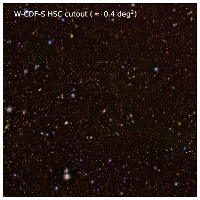
Figure 5: Left: Example “false-color” smoothed X-ray image cutout of W-CDF-S with field size $\approx 0.4$ deg² and central RA $=52.9^{\circ}$ and DEC $=-27.4^{\circ}$. Band 1+2, band 3, and band 4+5 are represented by the colors red, green, and blue, respectively. Redder sources are softer; bluer sources are harder. An asinh stretch is utilized. The large extended source toward the lower left is an X-ray cluster at $z=0.15$. Right: Example “false-color” optical image of W-CDF-S in the same sky area as that of the left panel. The $g$/$i$/$z$-band HSC image is represented by the color blue/green/red.

3.3 Simulations to assess catalog reliability

Similar to Chen et al. (2018), we perform Monte Carlo simulations of the X-ray observations in W-CDF-S and ELAIS-S1 to assess the reliability of the source catalogs. For each simulation, we generate mock X-ray sources using the Kim et al. (2007) log $N$-log $S$ relations. The minimum simulated flux is set to be 0.5 dex lower than the minimum detected flux; the maximum flux is set to be $10^{-11}$ erg cm^-2 s^-1. We then use CDFS-SIM to convert fluxes to PN/MOS count rates, and place sources at random sky positions, thus creating mock event files. The images are extracted in the same manner as the real ones. The background is simulated by re-sampling the original background map according to a Poisson distribution. A total of 10 simulations are created for each energy band. The same two-stage source-detection procedures are performed on the simulated data; the detected sources are matched to input sources within a $10^{\prime\prime}$ cut-off radius by minimizing the quantity $R^{2}$:

$$R^{2}=\big{(}\frac{\Delta{\rm RA}}{\sigma_{\rm RA}}\big{)}^{2}+\big{(}\frac{\Delta{\rm DEC}}{\sigma_{\rm DEC}}\big{)}^{2}+\big{(}\frac{\Delta{\rm RATE}}{\sigma_{\rm RATE}}\big{)}^{2},$$ (1)

where $\Delta{\rm RA}$/$\Delta{\rm DEC}$/$\Delta{\rm RATE}$ is the difference between the RA/DEC/count rate of matched detected sources and input sources; $\sigma_{\rm RA}$/$\sigma_{\rm DEC}$/$\sigma_{\rm RATE}$ is the uncertainty of the detected sources in RA/DEC/count rate. Detected sources without any input sources within $10^{\prime\prime}$ are considered to be spurious detections.

The left/right panel of Figure 6 presents the average spurious fraction ($f_{\rm spurious}$) as a function of det_ml in the full/soft/hard band for the W-CDF-S/ELAIS-S1 field obtained from the simulations we ran. To achieve $f_{\rm spurious}$ $\lesssim 1\%$ for the W-CDF-S field, a det_ml threshold of $\approx 3.5/3.5/9.5$ is needed for the full/soft/hard band. For the ELAIS-S1 field, a det_ml threshold of $\approx 4.0/4.0/8.0$ is required for the full/soft/hard band. In the soft band, the background levels are similar for the W-CDF-S and ELAIS-S1 fields. Thus, due to the slightly larger amount of exposure time in W-CDF-S than ELAIS-S1, the det_ml threshold in the soft band for the W-CDF-S field is slightly smaller than that for the ELAIS-S1 field. In the hard band, the background level for the W-CDF-S field is higher compared to the ELAIS-S1 field. Thus, the det_ml threshold in the hard band for the W-CDF-S field is larger than that for the ELAIS-S1 field. The source signal in the full band is typically dominated by the source signal from the soft band, so that the det_ml threshold in the full band is close to that in the soft band.

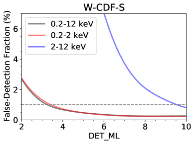
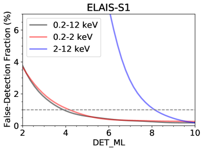
Figure 6: Left: The fraction of spurious sources as a function of det_ml threshold based on simulations. The horizontal dashed line marks a spurious fraction of 1%, which determines the det_ml thresholds adopted for W-CDF-S. Right: Similar to the left panel, but for the ELAIS-S1 field.

3.4 Astrometric accuracy

To estimate the positional accuracy of the detected XMM-Newton sources in the full/soft/hard band, we first matched the sources with optical catalogs. As described in Chen et al. (2018), directly matching X-ray sources to optical counterparts can be associated with a relatively high false-match rate ($\approx 18\%$). We therefore chose NWAY (Salvato et al. 2018; see Section 4 for a basic description of NWAY) to match XMM-Newton sources with optical/NIR counterparts with priors as described in Section 4 within 10^′′, using an iterative method. In the NIR, we use Spitzer data from the DeepDrill data release (Lacy et al., 2021) that includes the SERVS data (Mauduit et al., 2012), and VISTA data from the VIDEO data release in 2020 (M. Jarvis et al., private communication) for both the W-CDF-S and ELAIS-S1 fields. In the optical, we use HSC data from Ni et al. (2019) for W-CDF-S and DES DR2 data (Abbott et al., 2021) for ELAIS-S1 (see Table 1 for the survey descriptions). Since a small fraction of X-ray sources in the W-CDF-S field lack HSC coverage (see Figure 1), we add DES DR2 sources (Abbott et al., 2021) in the W-CDF-S field that have no HSC counterpart within 1 arcsec to the HSC catalog; this also provides optical coverage in the saturated regions of the HSC image. In the first iteration, we adopt the quadrature combination of the positional uncertainty derived from emldetect ($\sigma_{\rm eml}$) and a constant 0.5 arcsec systematic uncertainty as the positional uncertainty of XMM-Newton sources ($\sigma_{x}$). The positional uncertainties adopted for optical/NIR sources are listed in Table 4. We then select all the X-ray sources in W-CDF-S/ELAIS-S1 with HSC/DES counterparts that have $p_{\rm any}$ $>0.1$ (which is the threshold adopted in this work, corresponding to a false-match rate of $\sim 5\%$; see Section 4.3 and Figure 19). We also exclude $\approx 4\%$ X-ray sources and their matched optical counterparts that have positional offsets greater than 3$\sigma_{x}$ from the analysis. We fit the separations between X-ray sources and optical sources as a linear function of source counts ($C$) in W-CDF-S and ELAIS-S1, respectively, and then adjust the intercept so that 68% of the sources have positional offsets smaller than the expectation from the relation (see Figure 7 for the obtained relations in the full band). The intercept and slope are taken as the parameters for the empirical relation between the 68% positional-uncertainty radius ($r_{68\%}$) and the number of source counts:

$$\log_{10}r_{68\%}=\alpha\times\log_{10}C+\beta.$$ (2)

Following Chen et al. (2018), we define $\sigma_{x}$ to be the same as the uncertainties in RA and DEC ($\sigma_{\rm RA}=\sigma_{\rm DEC}=\sigma_{x}$), so that $\sigma_{x}$ = $r_{68\%}$/1.515 (see Pineau et al. 2017 for details). With the updated $\sigma_{x}$, we run NWAY again, iterating until the $\alpha$ and $\beta$ values become stable.

The distribution of $\sigma_{x}$ can be roughly approximated as a normal distribution. For the W-CDF-S field, the average $\sigma_{x}$ in the full/soft/hard band is 1.15/1.25/1.10 arcsec, with a standard deviation of 0.46/0.51/0.31 arcsec. For the ELAIS-S1 field, the average $\sigma_{x}$ in the full/soft/hard band is 1.15/1.21/1.15 arcsec, with a standard deviation of 0.51/0.55/0.34 arcsec. Since we assume $\sigma_{\rm RA}=\sigma_{\rm DEC}=\sigma_{x}$, the separation between X-ray sources and their optical counterparts should follow the Rayleigh distribution (with the scaling parameter $\sigma_{x}$). The distribution of the normalized separation (Separation/$\sigma_{x}$) between the full-band X-ray sources and their optical counterparts is presented in Figure 8, along with the Rayleigh distribution. The good agreement between the distribution of separation/$\sigma_{x}$ and the Rayleigh distribution indicates that our empirically derived $\sigma_{x}$ values are reliable indicators of the true positional uncertainties.

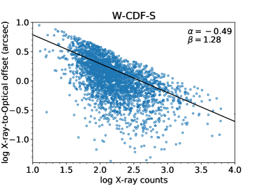
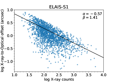
Figure 7: The positional offsets between detected X-ray sources in the full band and their matched optical counterparts vs. the full-band X-ray source counts number ($C$) in W-CDF-S (top) and ELAIS-S1 (bottom). The derived relation between $\log_{10}r_{68\%}$ and $C$ is marked as the black solid line.

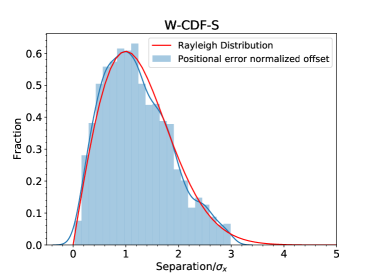
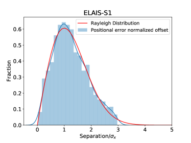
Figure 8: Comparison between the distribution of the separations between the full-band X-ray sources and their optical counterparts divided by $\sigma_{x}$ and the expected Rayleigh distribution (solid red curve) in W-CDF-S (top) and ELAIS-S1 (bottom). The solid blue curve represents the kernel-density estimation of the normalized separation distribution. The agreement between the two distributions indicates that our empirically derived $\sigma_{x}$ values are reliable.

3.5 The X-ray source catalogs

We present the schema of the X-ray source catalogs for the W-CDF-S and ELAIS-S1 fields in Appendix A. With the det_ml thresholds derived in Section 3.3, we detect 3512/3672/1118 sources in the full/soft/hard band in the W-CDF-S field, and 2328/2342/884 sources in the full/soft/hard band in the ELAIS-S1 field. These numbers only include point-like sources; sources that have $\geqslant 10$ improvements in the detection likelihood when detected as an extended source compared to the likelihood when detected as a point-like source are not included in our X-ray catalogs. To combine sources detected in the three energy bands, we first need to identify sources that are detected in more than one band. Two sources detected in different bands are considered to be the same if their angular separation is smaller than 10^′′, or the quadratic sum of the $99.73\%$ positional uncertainties from both bands. Then, we add sources that are only detected in a single band to the source list. We thus have a catalog of 4053/2630 unique point-like sources (see Figure 9 for the spatial distribution of sources) in the W-CDF-S/ELAIS-S1 field. In the W-CDF-S/ELAIS-S1 field, a total of 2262/1407 sources have more than 100 PN+MOS counts in the full band; 139/78 sources have more than 1000 X-ray counts in the full band (see Figure 11 for the counts distribution). For the W-CDF-S field, $\approx 5/12/1\%$ of the sources are only detected in the full/soft/hard band; for the ELAIS-S1 field, $\approx 5/10/1\%$ of the sources are only detected in the full/soft/hard band. We have performed visual examinations to ensure that no obvious sources are missing from the catalogs, and that there are no obvious false matches between different bands.

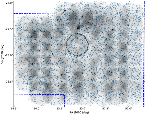
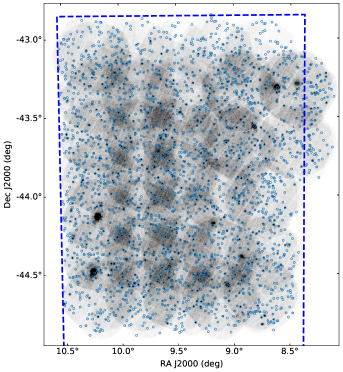
Figure 9: Left: Spatial distribution of the point-like X-ray detected sources in the W-CDF-S field (blue circles) projected on the smoothed full-band image. The blue dashed line encloses the region with forced optical-NIR photometry (Nyland et al. 2021). The black solid curve indicates the footprint of the 7 Ms CDF-S (Luo et al., 2017). W-CDF-S is larger than the CDF-S by a factor of $\approx 34$ in solid angle. Right panel: Spatial distribution of the point-like X-ray detected sources in the ELAIS-S1 field (blue circles) projected on the smoothed full-band image. The blue dashed line encloses the region with forced optical-NIR photometry (Zou et al., 2021).

When a source is not detected in all the bands, we estimated its count-rate upper limits in bands where the source is undetected. The minimum required source counts ($m$) for a source to be detected with the emldetect detection threshold ($P_{\rm random}$; det_ml $=-~{}lnP_{\rm random}$) at a given number of background counts ($B$) can be estimated by solving the following regularized upper incomplete $\Gamma$ function (Chen et al., 2018):

$$P_{\rm Random}=\frac{1}{\Gamma(m)}\int_{B}^{\infty}t^{m-1}e^{-t}dt.$$ (3)

Here, $B$ is estimated by summing the number of counts in $5\times 5$ pixels centered at the source position in the mosaicked background map. We note that the estimated $m$ corresponds to the Poisson detection likelihood of $P_{\rm Random}$, which is not necessarily equal to the detection likelihood from PSF fitting in emldetect. However, as the PSF fitting likelihood follows a 1:1 relation with the Poisson likelihood in general (Liu et al., 2020), our estimation roughly holds. With the estimated $m$, the count-rate upper limit is then calculated with the formula:

$${\rm RATE_{upper~{}limit}}=\frac{m-B}{t_{\rm exp}\times{\rm EEF}},$$ (4)

where $t_{\rm exp}$ represents the exposure time at the source position, and the encircled energy fraction (EEF) value corresponding to the 5 $\times$ 5 pixels centered at the source position is obtained from the EEF map. To derive the EEF map, we use psfgen to generate a series of PSF models for the three EPIC cameras, with different off-axis angles and different energies. These PSF models approximate the EEF as a function of the off-axis angle for different EPIC cameras at different energies. For each observation, an EEF map is generated for each EPIC camera. A mosaicked EEF map for different EPIC instruments at different energies is constructed (see Figure 10 for the soft-band EEF maps). The EEF value adopted in Equation 4 is the weighted EEF of EEF values at the source position for the three EPIC cameras, with the counts number in the band where the source is detected in each EPIC camera serving as the weight. Similarly, as exposure times in different EPIC cameras vary, the $t_{\rm exp}$ adopted in Equation 4 is the weighted $t_{\rm exp}$ (with the same weights as those utilized to calculate the weighted EEF).

Figure 10: Soft-band encircled energy fraction (in $5\times\ 5$ pixels) maps for the three EPIC cameras in W-CDF-S (left) and ELAIS-S1 (right). The gaps in the EEF map of MOS1 are due to its lost CCDs.

To convert the count rate to flux, we derive the effective power-law photon indices, $\Gamma_{\rm eff}$ (or the upper/lower limits of the indices), for X-ray sources from the hard-to-soft band ratios (or the lower/upper limits of the band ratios), assuming a power law modified by Galactic absorption. The band ratio is calculated as the ratio between the hard-band count rate and the soft-band count rate. The relation between the band ratio and $\Gamma_{\rm eff}$ is derived from the canned response files of EPIC cameras. The soft/hard/full-band flux of the source is derived from the soft/hard/full-band count rate in each EPIC camera assuming a power-law spectrum with the derived $\Gamma_{\rm eff}$; the weighted mean of fluxes obtained from all available EPIC cameras (the ratio between the count rate and the count-rate error in each camera is utilized as the weight) is reported as the flux of the source. For sources that are detected in the soft band but not in the hard band in W-CDF-S and ELAIS-S1, we stack their hard-band counts at the source positions to derive a stacked $\Gamma_{\rm eff}$, which is $\approx 1.9$ in W-CDF-S and $\approx 2.0$ in ELAIS-S1. The stacking is performed by summing all the counts in 5 $\times$ 5 pixels of the image centered at the source position, minus all the counts in 5 $\times$ 5 pixels of the background map centered at the source position, and then dividing by the EEF. Similarly, for sources that are detected in the hard band but not in the soft band, we stack their soft-band counts at the source positions to obtain a stacked $\Gamma_{\rm eff}$, which is $\approx 0.6$ for both W-CDF-S and ELAIS-S1. When the stacked $\Gamma_{\rm eff}$ value is consistent with the $\Gamma_{\rm eff}$ limit of a source, the stacked $\Gamma_{\rm eff}$ value is utilized to derive the flux; otherwise, the $\Gamma_{\rm eff}$ limit is utilized to derive the flux. When a source is only detected in the full band, $\Gamma_{\rm eff}=1.4$ (which is approximately the slope of the cosmic X-ray background spectrum; e.g., Marshall et al. 1980) is assumed to derive the flux.

The distributions of source counts in the soft, hard, and full bands and observed fluxes (i.e., fluxes only corrected for Galactic absorption) of the detected sources in the 0.5–2 keV, 2–10 keV, and 0.5–10 keV bands are displayed in Figure 11; we present the observed fluxes in the 0.5–2 keV, 2–10 keV, and 0.5–10 keV bands (calculated with the $\Gamma_{\rm eff}$ values derived in the previous paragraph) to enable direct comparisons with previous X-ray surveys (e.g., Cappelluti et al., 2009; Chen et al., 2018). The median observed fluxes of sources in the W-CDF-S field detected in the 0.5–2, 2–10, 0.5–10 keV bands are $5.4\times 10^{-15}$, $1.1\times 10^{-14}$, and $9.0\times 10^{-15}$ erg cm^-2 s^-1, respectively. The median observed fluxes of sources in the ELAIS-S1 field detected in the 0.5–2, 2–10, 0.5–10 keV bands are $6.6\times 10^{-15}$, $1.0\times 10^{-14}$, and $1.1\times 10^{-14}$ erg cm^-2 s^-1, respectively.

In Table 3, we compare the solid angle and number of detected X-ray sources for the whole XMM-SERVS survey with several other wide-field XMM-Newton surveys, showing the legacy value of XMM-SERVS.

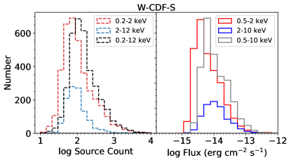
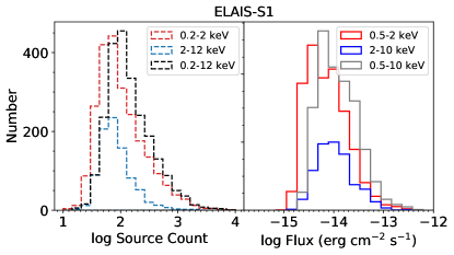
Figure 11: Left panels: The distributions of source counts in the soft (0.2–2 keV; red dashed), hard (2–12 keV; blue dashed), and full (0.2–12 keV; black dashed) bands. Right panels: The distributions of fluxes in the 0.5–2 keV (red), 2–10 keV (blue), and 0.5–10 keV (gray) bands.

Table 3: Comparison of selected wide-field XMM-Newton surveys.

Field	Area	Depth	Source	Reference
	(deg2)	(ks)	number
XMM-SERVS	13	30	11925	-
SXDS	1.14	40	1245	Ueda et al. (2008)
XMM-COSMOS	2	40	1887	Cappelluti et al. (2009)
XMM-XXL-N	25	10	14168	Chiappetti et al. (2018)
Stripe 82X	31.3	5	6181	LaMassa et al. (2016)

Columns from left to right: survey field, solid-angle coverage, median XMM-Newton PN depth across the field (in ks), number of sources detected, and example reference for the survey.

3.6 Survey sensitivity, sky coverage, and logN-logS

We create sensitivity maps in W-CDF-S and ELAIS-S1 in the 0.5–2, 2–10, and 0.5–10 keV bands following the methods in section 3.6 of Chen et al. (2018). We first bin the mosaicked background and exposure maps in the soft, hard, and full bands for each instrument by 3 $\times$ 3 pixels (which is the bin size recommended by the XMM-SAS task esensmap). For each pixel of the binned background map with a background counts number of $B$, the minimum required source counts ($m$) for a source to be detected with the emldetect detection threshold could be estimated from Equation 3. The sensitivity is calculated with the formula:

$$S=\frac{m-B}{t_{\rm exp}\times{\rm EEF}\times{\rm ECF}},$$ (5)

where energy conversion factors (ECFs) for different bands and different EPIC cameras are derived assuming a power-law spectrum with photon index $\Gamma=1.4$ modified by Galactic absorption. For X-ray sources in the W-CDF-S field, the adopted ECF values for PN/MOS1/MOS2 are 8.57/2.27/2.28, 1.10/0.38/0.38, and 3.00/0.86/0.87 counts s${}^{-1}/10^{-11}$erg cm^-2 s^-1, when converting count rates detected in the soft band to fluxes in the 0.5–2 keV band, count rates detected in the hard band to fluxes in the 2–10 keV band, and count rates detected in the full band to fluxes in the 0.5–10 keV band, respectively. For X-ray sources in the ELAIS-S1 field, the adopted ECF values for PN/MOS1/MOS2 are 8.03/2.21/2.21, 1.10/0.38/0.38, and 2.78/0.82/0.83 counts s${}^{-1}/10^{-11}$erg cm^-2 s^-1. For each EPIC camera in the soft/hard/full band, we generate a map for the $\frac{1}{t_{\rm exp}\times{\rm EEF}\times{\rm ECF}}$ term in Equation 5, and bin it by 3 $\times$ 3 pixels. As the effective area of PN is $\approx 2.5$ times the effective area of MOS1/MOS2, we combine the $\frac{1}{t_{\rm exp}\times{\rm EEF}\times{\rm ECF}}$ map of PN, MOS1, and MOS2 in each energy band with a weight of 2.5:1:1. Multiplying this merged map with the $m-B$ value at each pixel, we obtain the sensitivity map at 0.5–2/2–10/0.5–10 keV (see Figure 12). Our survey in the W-CDF-S field has flux limits of $1.9\times 10^{-15}$, $2.9\times 10^{-14}$, and $1.0\times 10^{-14}$ erg cm^-2 s^-1 over 90% of its area in the 0.5–2, 2–10, and 0.5–10 keV bands, respectively. Our survey in the ELAIS-S1 field has flux limits of $2.5\times 10^{-15}$, $3.2\times 10^{-14}$, and $1.3\times 10^{-14}$ erg cm^-2 s^-1 over 90% of its area in the 0.5–2, 2–10, and 0.5–10 keV bands, respectively. The sensitivity curves corresponding to the det_ml threshold for the 0.5–2/2–10/0.5–10 keV bands are shown in Figure 13.

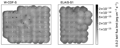
Figure 12: 0.5–2 keV band sensitivity maps in W-CDF-S (left) and ELAIS-S1 (right).

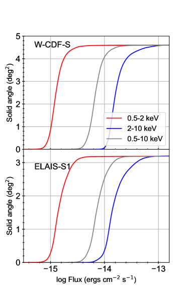
Figure 13: Sensitivity curves in the 0.5–2/2–10/0.5–10 keV band, calculated with the det_ml thresholds in Section 3.3.

Utilizing these sensitivity curves, we calculate the $\log N-\log S$ relations for our survey (see Figure 14). As can be seen in Figure 14, the $\log N-\log S$ relations in W-CDF-S and ELAIS-S1 are, in general, consistent with the relations reported in other studies (CDF-S 7 Ms, Luo et al. 2017; XMM-COSMOS, Cappelluti et al. 2009; COSMOS-Legacy, Civano et al. 2016; and Stripe 82X, LaMassa et al. 2016) within the measurement uncertainties.

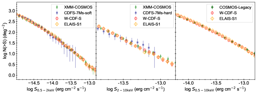
Figure 14: The $\log N-\log S$ relations for our catalogs in the 0.5–2 keV band (left), 2–10 keV band (middle), and 0.5–10 keV band (right). For comparison, $\log N-\log S$ relations from other X-ray surveys are shown (CDF-S 7 Ms, Luo et al. 2017; XMM-COSMOS, Cappelluti et al. 2009; and COSMOS-Legacy, Civano et al. 2016). The $\log N-\log S$ relations of our survey are generally consistent with those of previous studies.

4 Multiwavelength counterparts of X-ray sources

To identify the multiwavelength counterparts for our X-ray sources, we utilize the Bayesian catalog matching tool NWAY (Salvato et al., 2018), which adopts the distance and magnitude/color priors from multiple catalogs simultaneously to select the most probable counterpart, and allows for the absence of counterparts in some catalogs. NWAY has been widely utilized in matching XMM-Newton sources to multiwavelength counterparts (e.g., Salvato et al., 2018; Chen et al., 2018; Liu et al., 2020). Table 3 shows the optical/NIR catalogs utilized in this work. In Sections 4.1 and 4.2, we describe the magnitude/color priors utilized. In Section 4.3, we present the quality of the matched optical/NIR counterparts.

4.1 Obtaining priors from Chandra sources

As can be seen from Column 5 of Table 3, it is typical for an XMM-Newton source in our catalogs to have multiple optical/NIR sources located within the 99.73% positional uncertainty ($r_{99\%}$). Thus, to compute the magnitude/color priors of the expected counterparts of our X-ray sources, we make use of the Chandra counterparts of our XMM-Newton sources within the E-CDF-S, CDF-S, and the original $\approx 0.6$ deg² ELAIS-S1 regions (Feruglio et al., 2008; Xue et al., 2016; Luo et al., 2017), along with other sources reported in the Chandra Source Catalog (CSC) 2.0 (Evans et al., 2010), as Chandra detections have better positional accuracy than XMM-Newton detections. We select Chandra sources that are uniquely matched to sources in our X-ray catalogs within the 95% uncertainties (Chandra and XMM-Newton positional uncertainties are added in quadrature; the positional uncertainties of the Chandra sources are taken from the relevant Chandra catalogs). This approach ensures that the Chandra sources utilized to obtain the priors have similar flux levels as XMM-Newton sources in our catalogs. A total of 264/275 XMM-Newton sources are matched to a unique Chandra counterpart in W-CDF-S/ELAIS-S1. The fluxes and effective power-law indices of matched Chandra sources are in agreement with XMM-Newton sources. Only a small fraction ($\approx 4\%$) of XMM-Newton sources have $>1$ Chandra counterpart within the 95% positional uncertainties.

We search for optical/NIR counterparts within 5^′′ of these Chandra sources with NWAY, utilizing the magnitude priors in the $i$, $K_{s}$, and IRAC 3.6$\mu m$ bands generated from the “AUTO” method. We select only reliable counterparts with $p_{\rm any}$ $>$ 0.8 (which corresponds to a false-positive fraction of $\approx$ 5% for Chandra sources; the false-positive fraction is estimated by matching fake X-ray sources with optical/NIR counterparts; see Section 4.3 for the methods).

As expected from the spectral energy distributions (SEDs) of AGNs, the matched counterparts of Chandra sources occupy a different space in the IRAC [3.6] $-$ [4.5] vs. IRAC [3.6] $+$ [4.5] plane compared with other sources in the DeepDrill catalog (see Figure 15). A color and magnitude prior in the NIR has been widely used in the multiwavelength counterpart matching of X-ray sources (e.g., Chen et al. 2018; Liu et al. 2020). Similar to the approach described in Liu et al. (2020), we pixelate the IRAC [3.6] $-$ [4.5] vs. IRAC [3.6] $+$ [4.5] space into 50 $\times$ 50 pixels, and use a 2D Gaussian kernel estimate to generate the prior (“IRAC 2D prior” hereafter) for the counterparts of X-ray sources in our survey based on the positions of matched Chandra sources/other sources in the DeepDrill catalog on the IRAC [3.6] $-$ [4.5] vs. IRAC [3.6] $+$ [4.5] plane. We also compute the 1D IRAC [3.6] $-$ [4.5] and IRAC [3.6] + [4.5] priors utilizing a Gaussian kernel estimate; we compute the magnitude prior for the IRAC 3.6$\mu$m band solely as well (see Figure 16). We do not create VIDEO and HSC (or DES) color priors as done above for the IRAC color, because this action would introduce a bias against type II AGN (just as for most of the VIDEO, HSC, and DES sources that do not have an X-ray counterpart, type II AGNs are typically dominated by host-galaxy light in the optical; e.g., Liu et al. 2020). We do use a Gaussian kernel estimate to obtain magnitude priors for the HSC/DES $i$ band and VIDEO $K_{s}$ band (see Figure 16).

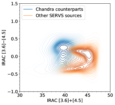
Figure 15: The IRAC [3.6] $-$ [4.5] vs. IRAC [3.6] $+$ [4.5] distribution of sources in the DeepDrill catalog that are matched to Chandra sources (blue contours), and the remaining DeepDrill sources (orange contours). The distribution of DeepDrill sources that have Chandra counterparts shows noticeable differences compared to other DeepDrill sources.

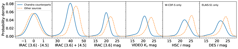
Figure 16: Kernel-density estimations of the IRAC 3.6 $\mu$m $-$ IRAC 4.5 $\mu$m color, IRAC 3.6 $\mu$m $+$ IRAC 4.5 $\mu$m magnitude, IRAC 3.6 $\mu$m magnitude, VIDEO $K_{s}$-band magnitude, and HSC/DES $i$-band magnitude distributions of the expected counterparts of X-ray sources in W-CDF-S and/or ELAIS-S1 (blue solid line) and the unmatched optical/NIR sources in the field (orange dashed line).

Table 4: Summary of multiwavelength counterpart matching results.

Catalog	Limiting Magnitude	Area	$\sigma$	$\overline{N_{99\%}}$	$f_{\rm matched}$	$f_{\rm reliable}$	$f_{\rm FP}$	$f_{\rm AP}$	False Rate	Identical Fraction
		(deg2)	(′′)					(Simulation)	(Simulation)	(Chandra)
(1)	(2)	(3)	(4)	(5)	(6)	(7)	(8)	(9)	(10)	(11)
W-CDF-S
DeepDrill	$3.6\mu$m $<23.1$	4.6	0.5	1.2	89.6%	85.2%	18.4%	81.0%	4.8%	96.9%
VIDEO	$K_{s}<23.8$	4.5	0.3	2.0	88.3%	82.7%	18.9%	78.8%	5.5%	92.2%
HSCa	$i<25.8$	4.6	0.1	2.3	95.5%	86.1%	20.8%	82.8%	4.6%	92.6%
Summary	-	-	-	-	100%	88.8%	22.3%	-	-	91.9%
ELAIS-S1
DeepDrill	$3.6\mu$m $<23.1$	3.2	0.5	1.2	90.5%	84.0%	19.2%	80.4%	4.9%	97.8%
VIDEO	$K_{s}<23.8$	3.0	0.3	2.1	85.1%	76.3%	19.5%	71.0%	7.9%	96.0%
DES	$i<24.6$	3.2	0.15	1.5	88.4%	80.8%	20.2%	76.5%	6.3%	97.0%
Summary	-	-	-	-	100%	87.0%	22.4%	-	-	95.2%

Col. 1: Catalog name. Col. 2: Magnitude limit. Col. 3: Survey area in the XMM-SERVS survey region (4.6 deg² for W-CDF-S and 3.2 deg² for ELAIS-S1). Col. 4: Positional uncertainty adopted for sources in this optical/NIR catalog. Col. 5: Average number of sources in this optical/NIR catalog within the 99.73% positional uncertainty ($r_{99\%}$) of the X-ray sources. Col. 6: Percentage of X-ray sources with at least one counterpart in this optical/NIR catalog within the 10″ search radius. Col. 7: Percentage of X-ray sources matched with the optical/NIR catalog that have $p_{\rm any}>0.1$, which we considered to be reliable matches. Col. 8: The fraction of false-positive matches with the optical/NIR catalog among the mock “isolated population” with a $p_{\rm any}$ threshold of 0.1. Col. 9: The fraction of X-ray sources in the “associated population” estimated based on simulations. Col. 10: False-matching rates for X-ray sources with $p_{\rm any}>0.1$ estimated from simulations. Col. 11: Fraction of the X-ray sources that have identical matching results with the optical/IR catalog when utilizing Chandra or XMM-Newton positions.
In the summary row, col. 6 represents the percentage of X-ray sources that have at least one of the DeepDrill, VIDEO, or HSC counterparts; col. 7 lists the total percentage of X-ray sources that have $p_{\rm any}>0.1$; col. 8 represents the total fraction of false-positive matches among the mock “isolated population”; col. 11 contains the fraction of X-ray sources that have identical matched counterparts in all optical and NIR catalogs utilizing Chandra or XMM-Newton positions.
Notes: (a). In a small fraction of the W-CDF-S area without HSC coverage (see Figure 1), we add DES sources (Abbott et al., 2021) to the HSC catalog.

4.2 Choosing the priors when performing source matching

Utilizing different combinations of the priors described above, we run NWAY with a maximum distance of 10^′′ to match detected X-ray sources with the optical/NIR catalogs listed in Table 4. We also generate mock X-ray sources that are 30^′′ away from any real X-ray sources with NWAY, thus assessing the false-positive fraction of X-ray sources that should not have counterparts (when different combinations of priors are adopted). This false-positive fraction is significantly larger than the expected false rate for the matched counterparts of X-ray sources in the catalog, as most of the actual X-ray sources in our catalog are expected to have optical/NIR counterparts (see Section 4.3 for details).

The completeness for real X-ray sources, and the false-positive fraction among the mock X-ray sources as a function of adopted $p_{\rm any}$ threshold when different combinations of priors are utilized are presented in Figure 17. We also compare the false-positive fraction directly with the completeness when the $p_{\rm any}$ threshold varies. At a given false-positive fraction, combining the following priors: IRAC 2D, $i$-band mag, and $K_{s}$-band mag, yields the highest completeness; at a given completeness, adopting these priors produces the lowest false-positive fraction. Thus, we match XMM-Newton sources with these priors. The percentages of XMM-Newton sources that are matched to each optical/NIR catalog are listed in Table 4, Column 6.

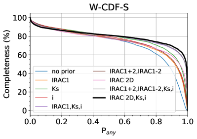
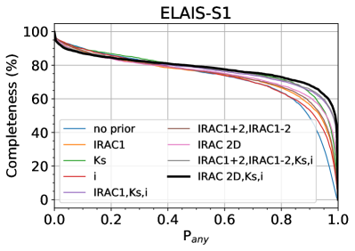
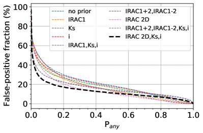
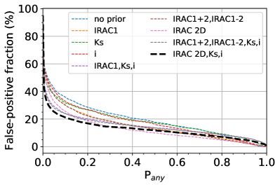
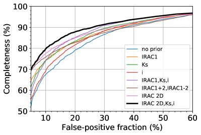
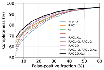
Figure 17: Top: Fraction of matched sources above the $p_{\rm any}$ threshold when different priors are adopted. Middle: Fraction of matched mock X-ray  sources above the $p_{\rm any}$ threshold when different priors are adopted. Bottom: Completeness vs. false-positive fraction when different priors are adopted.

4.3 Assessing the matched counterparts

The NWAY matching results can be assessed by investigating the subsample of XMM-Newton sources that have matched Chandra counterparts. We compare the matching results of Chandra sources with XMM-Newton sources. For W-CDF-S, the matched DeepDrill counterparts have a $\approx 97\%$ agreement; the matched VIDEO counterparts have a $\approx 92\%$ agreement; the matched HSC counterparts have a $\approx 93\%$ agreement (see Column 11 of Table 4). For ELAIS-S1, the matched DeepDrill counterparts have a $\approx 98\%$ agreement; the matched VIDEO counterparts have a $\approx 96\%$ agreement; the matched DES counterparts have a $\approx 97\%$ agreement. Examples of comparisons between the matching results utilizing Chandra and XMM-Newton positions are presented in Figure 18.

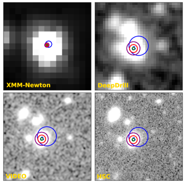
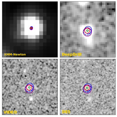
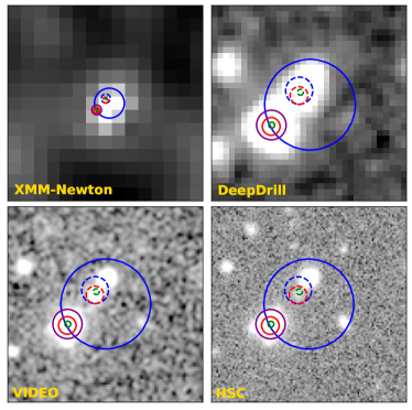
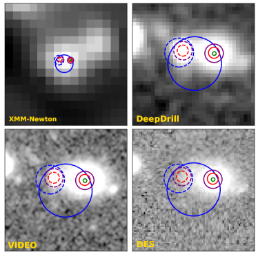
Figure 18: Illustrations of the comparison between the matching results using XMM-Newton positions vs. Chandra positions. Each set of four images shows cutouts from the smoothed XMM-Newton 0.2–12 keV image (top-left; $60^{\prime\prime}\times 60^{\prime\prime}$), DeepDrill IRAC 3.6$\mu$m band (top-right; $20^{\prime\prime}\times 20^{\prime\prime}$), VIDEO $K_{s}$-band (bottom-left; $20^{\prime\prime}\times 20^{\prime\prime}$), and HSC $i$-band (for the two W-CDF-S sets on the left) or DES $i$-band (for the two ELAIS-S1 sets on the right) (bottom right; $20^{\prime\prime}\times 20^{\prime\prime}$). X-ray positions are marked as blue circles with a 99.73% error radius, with the XMM-Newton positions indicated by solid lines and the Chandra positions indicated with dashed lines. DeepDrill counterparts matched utilizing XMM-Newton/Chandra positions are marked with solid/dashed purple circles; VIDEO counterparts are indicated with solid/dashed red circles; HSC/DES counterparts are identified with solid/dashed green circles. In most cases, the counterpart-matching results for XMM-Newton sources are identical to the results obtained using Chandra positions (see the top sets); there is a small fraction of sources where the XMM-Newton results do not agree with Chandra results (see the bottom sets).

We have also performed simulations in W-CDF-S and ELAIS-S1, respectively, to assess the results of multiwavelength counterpart matching with NWAY. Following Broos et al. (2011) and Chen et al. (2018), we consider our X-ray sources to have both an “associated population” (X-ray sources that do have a real counterpart in the corresponding optical/NIR catalog) and an “isolated population” (X-ray sources that do not have a real counterpart in the corresponding optical/NIR catalog).

The fraction of the associated population ($f_{\rm AP}$) can be calculated with the formula:

$$N_{\rm negative}=N_{\rm FN}\times f_{\rm AP}+N_{\rm TN}\times(1-f_{\rm AP}).$$ (6)

$N_{\rm negative}$ is the number of real X-ray sources that do not have a matched counterpart in an optical/NIR catalog; $N_{\rm FN}$ is the number of simulated X-ray sources that belong to the “associated population” but do not have a matched counterpart; $N_{\rm TN}$ is the number of mock X-ray sources that belong to the “isolated population” and are not matched to a counterpart as expected. As presented in Section 4.2, NWAY has a built-in function to simulate the isolated population and obtain $N_{\rm TN}$ with varying $p_{\rm any}$ thresholds. To simulate the associated population and calculate $N_{\rm FN}$ with varying $p_{\rm any}$ thresholds, we use a method similar to that in Section 4.2 of Chen et al. (2018). For X-ray sources that have $p_{\rm any}$ values above the adopted $p_{\rm any}$ threshold, we remove all their matched optical/NIR counterparts in the optical/NIR catalogs, and shift the position of all the remaining optical/NIR sources in the catalog by 1 arcmin in a random direction. We then generate fake optical/NIR “counterparts” for each X-ray source based on the X-ray and optical/NIR positional uncertainties, with all the priors utilized. When generating the optical/NIR positions for the W-CDF-S field, we use the positional uncertainty of X-ray sources and HSC sources to simulate HSC positions from the expected Rayleigh distribution of offsets. The generated HSC positions are utilized to simulate the positions of DeepDrill/VIDEO sources, assuming a Gaussian distribution for the offsets between HSC sources with their DeepDrill/VIDEO counterparts (the standard deviation of the Gaussian distribution is derived from all the matched DeepDrill/VIDEO sources with HSC sources within 1^′′). For the ELAIS-S1 field, DES sources are simulated instead of HSC sources. After that, we run NWAY to obtain $N_{\rm FN}$ among the associated population, thus obtaining $f_{\rm AP}$ by solving Equation 6. With $f_{\rm AP}$, we could obtain the expected false rate ($f_{\rm False}$) of matched counterparts with varying $p_{\rm any}$ thresholds:

$$f_{\rm False}=(N_{\rm IM}\times f_{\rm AP}+N_{\rm FP}\times(1-f_{\rm AP}))/(N_{\rm positive}).$$ (7)

$N_{\rm IM}$ is the number of incorrect matches among the simulated associated X-ray sources; $N_{\rm FP}$ is the number of false positives among the mock isolated X-ray sources. Figure 19 presents $f_{\rm False}$ as a function of the $p_{\rm any}$ threshold adopted. Similar to the finding in Chen et al. (2018), the matched IRAC counterparts have the smallest $f_{\rm False}$ among all the optical/NIR catalogs.

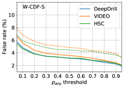
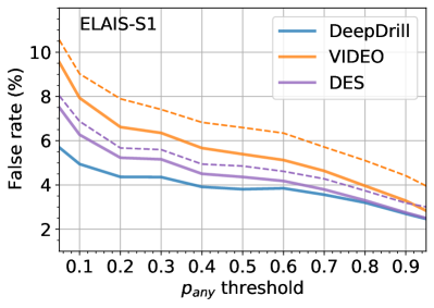
Figure 19: Left: False rate of matched DeepDrill/VIDEO/HSC counterparts as a function of $p_{\rm any}$ threshold adopted (blue/orange/green solid lines) when matching X-ray sources in W-CDF-S to all the optical/IR catalogs simultaneously. The orange/green dashed lines represent the false rates when matching X-ray sources to VIDEO/HSC sources based on their distances to the matched DeepDrill counterparts (when available). Right: False rate of matched DeepDrill/VIDEO/DES counterparts as a function of $p_{\rm any}$ threshold adopted (blue/orange/purple solid lines) when matching X-ray sources in ELAIS-S1 to all the optical/IR catalogs simultaneously. The orange/purple dashed lines represent the false rates when matching X-ray sources to VIDEO/DES sources based on their distances to the matched DeepDrill counterparts (when available).

In Section 4.2 of Chen et al. (2018), when SERVS counterparts are available for X-ray sources, other optical/NIR counterparts are selected based on matching them with the matched SERVS counterparts. We also calculate the $f_{\rm False}$ for VIDEO and HSC (or DES) with the following methodology: when an X-ray source has a DeepDrill counterpart, we identify VIDEO and HSC (or DES) counterparts purely based on the distance from the DeepDrill counterpart. The results are presented in Figure 19 as the dashed lines. For VIDEO and HSC (or DES) counterparts, the obtained false rates are slightly higher by $\approx 1$–2%, revealing the advantages of matching multiple optical/NIR catalogs to XMM-Newton sources simultaneously.

In the released catalogs, we do not apply any $p_{\rm any}$ threshold for the identified multiwavelength counterparts with match_flag = 1 (which indicates that this counterpart is the primary counterpart with the highest likelihood). However, a $p_{\rm any}$ threshold of at least 0.1 is suggested for catalog users so that the false rate of the optical/NIR counterparts is $\sim 5$% (see Table 4, Column 10). 3600/2288 X-ray sources in W-CDF-S/ELAIS-S1 have $p_{\rm any}$ $>0.1$, which is $\approx 89\%$/87% of the total X-ray sources detected (see Table 4, Column 7). For the analyses in Sections 5 and 6 where the optical/NIR counterparts of X-ray sources are utilized, we only use X-ray sources with $p_{\rm any}$ $>0.1$ counterparts. Figure 20 displays the offsets between X-ray sources (that have $p_{\rm any}$ $>0.1$) with their optical/NIR counterparts. Following a priority established based on the survey positional uncertainty, we use the HSC (or DES), VIDEO, or DeepDrill positions as the location of optical/NIR counterparts. Figure 20 also presents histograms of positional offsets when $\sigma_{x}$ varies, which demonstrates that our estimation of $\sigma_{x}$ from the empirical relation is reliable in general: since $r_{68\%}$ = $\sigma_{x}\times$ 1.515 (see Section 3.4), we expect the median positional offset in different $\sigma_{x}$ bins to increase with $\sigma_{x}$, and roughly 68% of the sources in a given $\sigma_{x}$ bin have positional offsets less than the median $r_{68\%}$ in this bin. Compared to many previous XMM-Newton survey catalogs (e.g., Chen et al. 2018; Liu et al. 2020), this work has substantially reduced the X-ray positional uncertainty and decreased the offset between X-ray sources and their optical/NIR counterparts.

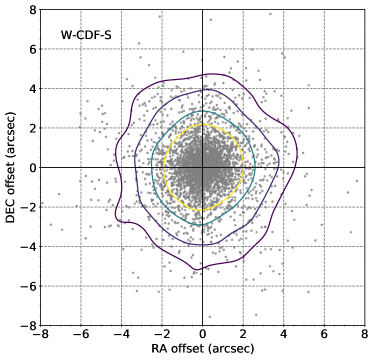
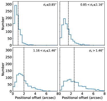
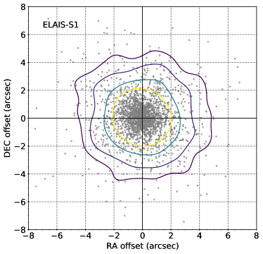
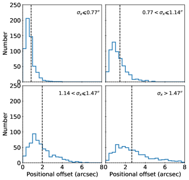
Figure 20: Left: The distribution of DEC offset vs. RA offset for X-ray sources in W-CDF-S (top) or ELAIS-S1 (bottom) and their optical/NIR counterparts, with contours indicating the isodensity levels that include 68%, 80%, 90%, and 95% of sources. Right: Histograms of positional offsets between X-ray sources in W-CDF-S (top) or ELAIS-S1 (bottom) (that are divided into four bins based on $\sigma_{x}$) and their matched optical/NIR counterparts. The vertical dashed line in each panel represents the median $r_{68\%}$ ($r_{68\%}$ = 1.515$\sigma_{x}$; see Section 3.4) value in each bin.

5 Redshifts

5.1 Spectroscopic redshifts

In addition to the extensive photometric data (see Table 1), there are a number of spectroscopic surveys in the W-CDF-S/ELAIS-S1 region (see Table 5). We match X-ray sources to these spectroscopic redshifts (spec-$z$s) utilizing the positions of matched optical/NIR counterparts: we search for the nearest spectroscopic redshift position that is within 1^′′ of these optical/NIR counterparts. When an X-ray source is matched to multiple spec-$z$s, we choose redshifts using the priority order in Table 5 (which is ranked based on the spectral resolution, as the accuracy of spec-$z$s is significantly dependent upon the spectral resolution; see Note (a) of Table 5 for more detail). Most of the spectroscopic surveys in Table 5 have resolution ¿ 100. As for the low-resolution PRIMUS survey, we only adopt the $Q$ $\geqslant 3$ ($Q$ is the redshift-quality flag provided by Coil et al. 2011) objects. Before matching X-ray sources to the PRIMUS catalog, we utilize the spec-$z$ compilation in the HELP database (Shirley et al., 2019), which provides several additional spec-$z$s.

In the W-CDF-S catalog, 919 ($\approx 23\%$) X-ray sources are matched to spec-$z$s ($\approx 750$ of them are outside of the E-CDF-S region), ranging from 0 to 4.56. In the ELAIS-S1 catalog, 585 ($\approx 22\%$) X-ray sources are matched to spec-$z$s, ranging from 0 to 4.04 ($\approx 300$ of them are outside of the original $\approx 0.6$ deg² ELAIS-S1 region). About $84\%$/$98\%$ of the matched spec-$z$ measurements are from catalogs that have spectroscopic classification for AGNs available in W-CDF-S/ELAIS-S1. Figure 21 shows the distribution of these spec-$z$s. In the future, there will be more public spectroscopic redshifts from surveys including CSI (e.g., Kelson et al., 2014), DEVILS (e.g., Davies et al., 2018; Thorne et al., 2020), DESI (e.g., Levi et al., 2019), MOONS (e.g., Maiolino et al., 2020), and WAVES (e.g., Driver et al., 2019).

Table 5: Spectroscopic-redshift catalogs used in this work, listed with priority from high to low.

Catalog	Instrument	Survey	Spectral	Targeting	Area	$N_{\rm matched}$	$N_{\rm assigned}$	Reference
		Sensitivity	Resolution	Fields	(deg2)
(1)	(2)	(3)	(4)	(5)	(6)	(7)	(8)	(9)
W-CDF-S
OzDES∗	AAOmega	$r\lesssim 22.5$	$\sim$1500	DES-SN C1,C2,C3	9	406	406	Lidman et al. (2020)
ATLAS∗	AAOmega	$R<22$	$\sim$1300	CDF-S	2.96	155	97	Mao et al. (2012)
BLAST∗	AAOmega	-	$\sim$1300	GOODS-South	3	47	21	Eales et al. (2009)
6dFGS	UKST	$K\lesssim$ 12.65	$\sim$1000	The Southern Sky	17,000	13	4	Jones et al. (2009)
2dFGRS	AAOmega	$\rm b_{J}<19.45$	$\sim$800	SGP strip	2000	30	5	Colless et al. (2001)
ACES	IMACS	$R<24.1$	$\sim$750	CDF-S	0.25	80	61	Cooper et al. (2012)
-	VIMOS/DEIMOS	R $<$ 25	$\sim$180/580	E-CDF-S	0.33	143	70	Silverman et al. (2010)
PRIMUS∗a	IMACS	$i\lesssim 23.5$	$\sim$30	CDFS-SWIRE,CALIB	2.1	349	252	Coil et al. (2011)
ELAIS-S1
OzDES∗	AAOmega	$r\lesssim 22.5$	$\sim$1500	DES-SN E1,E2	6	293	293	Lidman et al. (2020)
ATLAS∗	AAOmega	$R<22$	$\sim$1300	ELAIS-S1	4.69	46	30	Mao et al. (2012)
6dFGS	UKST	$K\lesssim$ 12.65	$\sim$1000	The Southern Sky	17,000	10	6	Jones et al. (2009)
2dFGRS	AAOmega	$\rm b_{J}<19.45$	$\sim$800	SGP strip	2000	5	1	Colless et al. (2001)
-∗	EFOSC, FORS2	-	$>$260	ELAIS-S1	0.6	129	106	Feruglio et al. (2008)
-∗	VIMOS	$R<24.2$	$\sim$210	ELAIS-S1	0.6	134	22	Sacchi et al. (2009)
PRIMUS∗a	IMACS	$i\lesssim 23.5$	$\sim$30	ELAIS-S1	0.9	223	123	Coil et al. (2011)

Col. 1: Redshift survey name. ^∗ marks redshift surveys where spectroscopic classification for AGNs is available (or partially available). Col. 2: Survey instrument. Col. 3: Survey sensitivity. Col. 4: Spectral Resolution. Col. 5: Targeted fields. Col. 6: Survey area. Col. 7: Total number of redshifts matched to the X-ray sources in the catalog. Col. 8: Total number of redshifts assigned to the X-ray sources in the catalog. Col. 9: Reference.
Notes: (a). The low-resolution PRIMUS survey greatly increases the sample with spectroscopic redshifts, although its measurements are not as accurate as other spectroscopic surveys listed and should be used with appropriate caution. For X-ray sources in our catalog, when both spec-$z$ measurements from PRIMUS and from other high-resolution spectroscopic surveys are available, $\approx 16\%$ of them have $\mathopen{|}\Delta z\mathclose{|}/(1+z_{\rm spec,high-resolution})>0.15$.

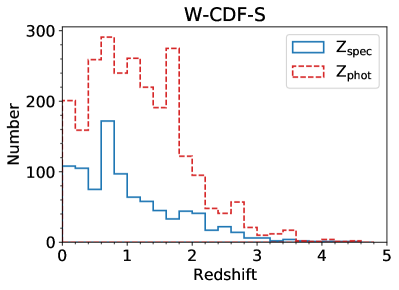
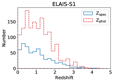
Figure 21: Distributions of the spectroscopic/photometric redshifts of X-ray sources that have spectroscopic/high-quality photometric redshift measurements (see Section 5) in the W-CDF-S and ELAIS-S1 fields, represented by the blue/red histograms (plotted respectively).

5.2 Photometric redshifts

Photometric redshifts (photo-$z$s) for X-ray sources in this work are derived from SEDs provided by the forced-photometry catalogs in the $4.5/3\rm~{}deg^{2}$ area covered by VIDEO in W-CDF-S/ELAIS-S1 (Nyland et al. 2021; Zou et al. 2021); these catalogs were generated utilizing The Tractor (Lang et al., 2016). The Tractor derives consistent flux measurements in all bands with priors of source positions and surface-brightness profiles obtained from a fiducial band. As can be seen in Figure 9, most ($\approx 95\%$) of our X-ray catalog areas are covered by these catalogs. The forced-photometry catalogs are generated following the methods in Nyland et al. (2017), where prior measurements of source positions and surface-brightness profiles from a fiducial VIDEO band (that has high resolution) are employed to model and fit the fluxes at other bands. The photometric bands utilized in W-CDF-S include the $u$, $g$, $r$ and $i$ bands in VOICE; $g$, $r$, $i$ and $z$ bands in HSC; $Z$, $Y$, $J$, $H$, and $K_{s}$ bands in VIDEO; and 3.6$\mu m$ and 4.5$\mu m$ bands in DeepDrill (see Table 1 for the survey information). In total, 3319 X-ray sources in W-CDF-S have forced-photometry measurements. For the HSC bands, we only utilize “clean” HSC photometry (see Ni et al. 2019 for details). For a band that is included in two surveys ($g$/$r$/$i$), the scatter in two sets of photometry is small ($\approx 0.2$ dex), and both detections are utilized in the photo-$z$ calculation. The photometric bands utilized in ELAIS-S1 include the $g$, $r$, $i$, $z$, and $Y$ bands in DES; $B$, $V$, and $R$ bands in ESIS; $u$ band in VOICE; $Z$, $Y$, $J$, $H$, and $K_{s}$ bands in VIDEO; and 3.6$\mu m$ and 4.5$\mu m$ bands in DeepDrill (Zou et al., 2021). In total, 2001 X-ray sources in ELAIS-S1 have forced-photometry measurements. When matching X-ray sources to the forced-photometry catalog, we utilize the position of their matched VIDEO counterparts. Galactic extinction corrections are applied to the photometry utilized (see Zou et al. 2021 for details).

Photo-$z$s for X-ray sources that are BL AGNs or non-BL AGNs are derived separately in our work. Here, BL AGNs are identified via classifications from spectroscopic surveys or the SED_BLAGN_FLAG $=1$ flag in this work (see Appendix B for details of selecting BL AGN candidates through observed-frame SEDs; sources marked with SED_BLAGN_FLAG $=1$ are likely to be BL AGNs). Photo-$z$s of X-ray sources that are not BL AGNs are provided in Zou et al. (2021) for both the W-CDF-S and ELAIS-S1 fields, which use the default templates of the SED-fitting code EAZY (Brammer et al., 2008). In W-CDF-S, 1792 of the matched photo-$z$s ($\approx 68\%$) have $Q_{z}<1$ ($Q_{z}$ evaluates the quality of the photo-$z$; see equation 8 of Brammer et al. 2008), which are considered to be of high quality. There are 455 sources with both spec-$z$ and $Q_{z}<1$ photo-$z$ measurements, which are utilized to assess the reliability of the photo-$z$s. The normalized median absolute deviation (NMAD) is $\sigma_{\rm NMAD}=0.04$, and the outlier fraction ($f_{\rm outlier}$; defined as $\Delta z/(1+z_{\rm spec})>0.15$, see Zou et al. 2021) is $6.8\%$; these numbers are similar to the photometric-redshift reliability in Chen et al. (2018). The distribution of $\mathopen{|}\Delta z\mathclose{|}/(1+z_{\rm spec})$ is given in Figure 22; the distribution of phot-$z$ vs. spec-$z$ is also presented in Figure 22. In ELAIS-S1, 1020 ($\approx 65\%$) of the photo-$z$s have $Q_{z}<1$. Among 230 sources with both spec-$z$ and $Q_{z}<1$ photo-$z$ measurements, the comparison between spec-$z$ and photo-$z$ produces $\sigma_{\rm NMAD}=0.03$ and $f_{\rm outlier}=5.2\%$ (see Figure 22).

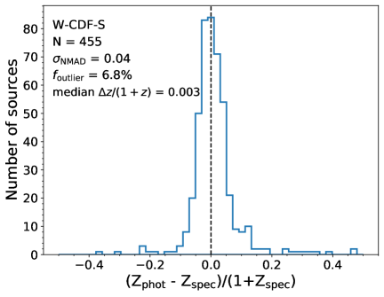
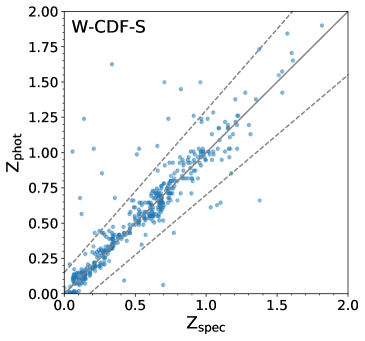
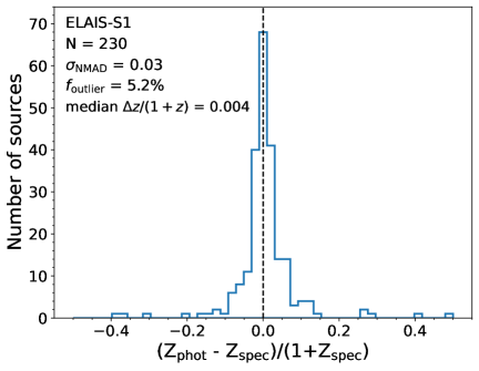
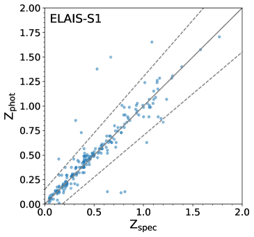
Figure 22: Left: Histogram of the fractional difference between the EAZY high-quality photo-$z$s and the spec-$z$s. Right: Comparison between the EAZY high-quality photo-$z$s and the spec-$z$s. The gray solid line represents the $z_{\rm spec}=z_{\rm phot}$ relation; the gray dashed lines represent the $\mathopen{|}\Delta z\mathclose{|}/(1+z_{\rm spec})=0.15$ boundary.

For the $\approx 760$/430 SED_BLAGN_FLAG $=1$ objects and the $Q_{z}\geqslant 1$ SED_BLAGN_FLAG $=0.5$ objects (sources marked with SED_BLAGN_FLAG $=0.5$ are possibly BL AGNs; see Appendix B) in W-CDF-S/ELAIS-S1, we utilized an SED library designed for fitting AGN-dominated sources (Salvato et al., 2009, 2011) with 30 templates in total to estimate the photo-$z$ of these BL AGN candidates with LePhare (Arnouts et al., 1999; Ilbert et al., 2006). As the characterization of AGN-dominated sources can be substantially improved when the Lyman break is detected (the optical-to-NIR SED of BL AGNs roughly follows a featureless power law, which may produce large errors for photometric redshifts derived from the template fitting), we match the positions of the optical/NIR counterparts of X-ray sources to the GALEX catalog (Martin et al., 2005) with a matching radius of 1^′′, and utilize the NUV and FUV fluxes when available. This approach allows the Lyman break to be detected at redshifts as low as $z=0.7$ (when the FUV flux is available) or $z=1.5$ (when the NUV flux is available). $\chi_{\rm red}^{2}<2$ and band number $>10$ are utilized to select high-quality photo-$z$ estimates ($\approx 74\%$ of them have high-quality photo-$z$). BL AGNs identified in spectroscopic surveys that have high-resolution ($>100$) spec-$z$ measurements are utilized to assess the LePhare photo-$z$ quality. Among these 174/138 sources in W-CDF-S/ELAIS-S1, 130/102 have high-quality LePhare photo-$z$ measurements utilizing the method above. A comparison between these spec-$z$ and photo-$z$ measurements produces $\sigma_{\rm NMAD}\approx 0.07$ and $f_{\rm outlier}\approx 18\%$ for W-CDF-S, and $\sigma_{\rm NMAD}\approx 0.06$ and $f_{\rm outlier}\approx 20\%$ for ELAIS-S1 (see Figure 23). However, as noted in Salvato et al. (2009), the photo-$z$ performance deteriorates when a source is fainter in the optical. For the BL AGNs with spec-$z$ measurements, the median $i$-band mag is $\approx 20$; this brightness is $\approx 22$ for BL AGN candidates without spec-$z$ measurements. In addition, only $\approx 40\%$ of the SED_BLAGN_FLAG $=1$ objects and the $Q_{z}\geqslant 1$ SED_BLAGN_FLAG $=0.5$ objects are matched to GALEX sources; this number is $\approx 85\%$ for spectroscopically confirmed BL AGNs. Thus, caution is advised when using LePhare photo-$z$ measurements for SED_BLAGN_FLAG $=0.5$ or $1$ sources.

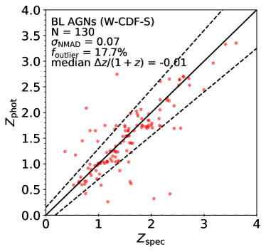
Figure 23: The comparison between the photo-$z$s and the spec-$z$s of broad-line AGNs that have both high-quality photo-$z$ from LePhare and resolution $>100$ spec-$z$ measurements. The black solid line represents the $z_{\rm spec}=z_{\rm phot}$ relation; the black dashed lines represent the $\mathopen{|}\Delta z\mathclose{|}/(1+z_{\rm spec})=0.15$ boundary.

Combining all the information above, we report the high-quality photo-$z$ measurements in the column PHOTOZ_BEST (see Appendix A): $Q_{z}<1$ EAZY photo-$z$ measurements are adopted for sources that have SED_BLAGN_FLAG $<1$ and are not identified as BL AGNs in spectroscopic surveys (1792 in W-CDF-S and 1020 in ELAIS-S1); high-quality LePhare photo-$z$ measurements are adopted for spectroscopically identified BL AGNs, SED_BLAGN_FLAG $=1$ objects, and SED_BLAGN_FLAG $=0.5$ objects without $Q_{z}<1$ EAZY photo-$z$ measurements (738 in W-CDF-S and 460 in ELAIS-S1). The catalog has high-quality photo-$z$ measurements for 1833/1117 X-ray sources in W-CDF-S/ELAIS-S1 without spec-$z$ measurements. The cumulative histogram of the $i$-band magnitude of X-ray sources with either spec-$z$ measurements or high-quality photo-$z$ measurements is presented in Figure 24.

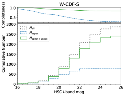
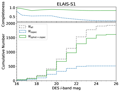
Figure 24: The cumulative distributions of the HSC/DES $i$-band magnitudes for $i$-band detected X-ray sources in W-CDF-S/ELAIS-S1 located within the region with forced photometry (gray dotted histogram), X-ray sources that have spec-$z$ measurements (blue dashed histogram), and X-ray sources that have either spec-$z$ or high-quality photo-$z$ measurements (green solid histogram). The blue dashed/green solid curve in the top panels is the fraction of X-ray sources in the region with forced photometry with spec-$z$/high-quality photo-$z$ or spec-$z$ measurements as a function of $i$-band magnitude. Objects without spec-$z$ or high-quality photo-$z$ measurements are SED_BLAGN_FLAG $=0$ objects with EAZY $Q_{z}>1$ or SED_BLAGN_FLAG $>0$ objects with LePhare $\chi^{2}_{\rm red}\geqslant 2$ or band number $\leqslant 10$.

6 Source properties and classification

For the 919/585 X-ray sources with spec-$z$ measurements and 1833/1117 X-ray sources with high-quality EAZY or LePhare photo-$z$ measurements (but lacking spec-$z$ measurements) in W-CDF-S/ELAIS-S1, we estimate their X-ray luminosity at rest-frame 2–10 keV ($L_{2-10\rm~{}keV}$) assuming a power-law spectrum with $\Gamma_{\rm eff}=1.8$ (which is a typical power-law photon index for AGNs; e.g., Lanzuisi et al. 2013; Yang et al. 2016; Liu et al. 2017) modified by Galactic absorption, utilizing source count rates in the priority order of hard band, full band, and soft band. This prioritization minimizes X-ray absorption effects. Figure 25 displays the distribution of $L_{2-10\rm~{}keV}$, as well as the $L_{2-10\rm~{}keV}$ vs. $z$ distribution. In Figure 26, we show the $L_{2-10\rm~{}keV}$ vs. $z$ distribution for the whole XMM-SERVS survey, and compare it with distributions from selected deep pencil-beam X-ray surveys (CDF-S; Luo et al. 2017; CDF-N; Xue et al. 2016) and shallower X-ray surveys over wider areas (XMM-XXL North; e.g., Menzel et al. 2016; Stripe 82X; e.g., Ananna et al. 2017; LaMassa et al. 2019). While deep pencil-beam surveys can detect less-luminous X-ray sources, the AGN sample size provided by the XMM-SERVS survey is substantially larger than the sample size these deep surveys could provide. When compared to shallower X-ray surveys over wider areas, we can see that the XMM-SERVS survey detects a significantly larger number of moderate-luminosity AGNs at log $L_{\rm X}$ $\sim 42$–44; also, due to the superb multiwavelength coverage of XMM-SERVS, the overall number of detected X-ray sources with reliable redshift measurements is larger at all redshifts. The $L_{2-10\rm~{}keV}$ vs. $z$ coverage of XMM-SERVS is similar to that of the Chandra COSMOS-Legacy survey (e.g., Marchesi et al., 2016), though the Chandra COSMOS-Legacy survey is somewhat deeper: the peak of the log $L_{2-10\rm~{}keV}$ distribution of X-ray sources in the Chandra COSMOS-Legacy survey is $\approx 0.5$ dex smaller than that of X-ray sources in XMM-SERVS. At the same time, the sample size of AGNs with reliable $L_{\rm X}$ estimation provided by XMM-SERVS is $\approx 3$ times that of the Chandra COSMOS-Legacy survey.

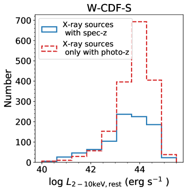
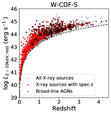
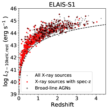
Figure 25: Left: The distribution of rest-frame 2–10 keV X-ray luminosity for X-ray sources with spec-$z$ measurements (blue solid histogram) and X-ray sources without spec-$z$ measurement but having high-quality photo-$z$ measurements (red dashed histogram), respectively. Right: The $L_{2-10\rm~{}keV}$ vs. $z$ distribution of all X-ray sources with spec-$z$ or high-quality photo-$z$ measurements (gray dots). X-ray sources with spec-$z$ measurements are marked by the red circles; among these sources, broad-line AGNs are marked as black pluses. The full-band sensitivity limit generated assuming $\Gamma_{\rm eff}=1.8$ is represented by the black dashed line.

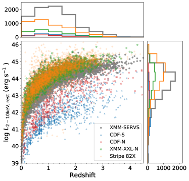
Figure 26: The $L_{2-10\rm~{}keV}$ vs. $z$ distribution of X-ray sources with spec-$z$ or high-quality photo-$z$ measurements in the full XMM-SERVS survey (gray dots). For comparison, the $L_{2-10\rm~{}keV}$ vs. $z$ distributions of X-ray sources in CDF-S (Luo et al., 2017), CDF-N (Xue et al., 2016), XMM-XXL North (e.g., Menzel et al., 2016), and Stripe 82X (e.g., Ananna et al., 2017; LaMassa et al., 2019) are shown as blue triangles, red crosses, green diamonds, and orange pluses, respectively. The distributions of $z$ for X-ray sources in the survey fields mentioned above are shown in the top sub-panel, with colors the same as those in the legend; the distributions of $L_{2-10\rm~{}keV}$ are shown in the right sub-panel, with colors the same as those in the legend.

We also perform basic AGN selection for X-ray sources in our catalogs following criteria from section 2.3 of Brandt & Alexander (2015) and references therein. The specific criteria utilized are the following:

1. Identified as broad-line AGNs in spectroscopic surveys (280 AGNs in W-CDF-S; 208 AGNs in ELAIS-S1).

2. Has observed $L_{2-10\rm keV}>3\times 10^{42}~{}\rm erg~{}s^{-1}$ (in the rest frame) when spec-$z$ measurements or high-quality EAZY or LePhare photo-$z$ measurements are available (2459 AGNs in W-CDF-S; 1511 AGNs in ELAIS-S1).

3. Has a power-law effective photon index $\Gamma\leqslant 1$ (412 AGNs in W-CDF-S; 314 AGNs in ELAIS-S1; see Figure 27). This criterion helps select hard X-ray sources that are heavily obscured, which are likely AGNs rather than X-ray binary populations (e.g., Alexander et al., 2005; Brandt & Alexander, 2015).

4. Identified as AGNs when utilizing X-CIGALE to perform SED template-fitting in Appendix B (2717 AGNs in W-CDF-S; 1684 AGNs in ELAIS-S1). AGNs selected via this SED-based selection method already include AGNs selected from empirical methods that use large X-ray-to-optical or X-ray-to-NIR flux ratios: $\log f_{x}/f_{i}>-1$ or $\log f_{x}/f_{Ks}>-1.2$ (see Figure 28). For the small fraction of X-ray sources that are not located within the VIDEO footprint that has forced photometry from optical to NIR available, we adopt large X-ray-to-optical flux ratios ($\log f_{x}/f_{i}>-1$) to identify AGNs (126 AGNs in W-CDF-S; 109 AGNs in ELAIS-S1).

5. Have red MIR colors (obtained from the four-band IRAC data) that meet the AGN criteria in Lacy et al. (2004), Stern et al. (2005), or Donley et al. (2012). Among 1897/1042 X-ray sources in W-CDF-S/ELAIS-S1 that are detected in four IRAC bands (as reported in Spitzer Data Fusion DR1; Vaccari 2015), 1441 objects in W-CDF-S ($\approx 76\%$) and 810 objects in ELAIS-S1 ($\approx 78\%$) are MIR-selected AGNs. Only 52/38 of these objects in W-CDF-S/ELAIS-S1 are not already identified as AGNs with the first four methods (see Figure 29). If we only adopt the conservative selection criteria from Donley et al. (2012), only 24/16 additional AGNs are identified in W-CDF-S/ELAIS-S1 via the MIR approach.

6. Have ATLAS radio counterparts and SWIRE 24$\mu$m counterparts and satisfy the $q_{24}<0$ radio AGN selection criterion in Donley et al. (2005), where $q_{24}$ is defined as ${\rm log}(S_{\rm 24,obs}/S_{\rm 1.4~{}GHz,obs})$ ($S_{\rm 24,obs}$ is the SWIRE 24 $\mu$m flux density, and $S_{\rm 1.4~{}GHz,obs}$ is the 1.4 GHz flux density). Among 213 objects in W-CDF-S and 86 objects in ELAIS-S1 that have both 24 $\mu$m and 1.4 GHz counterparts detected, 49/15 objects in W-CDF-S/ELAIS-S1 are identified as AGNs. 11/0 of these objects in W-CDF-S/ELAIS-S1 are not already identified as AGNs via the first four methods.

The combination of all these methods identifies 3186 AGNs in W-CDF-S and 1985 AGNs in ELAIS-S1, which is $\approx 89\%$/87% of X-ray sources matched to multiwavelength counterparts with $p_{\rm any}$ $>0.1$. The non-AGN X-ray sources could be attributed to stars, bright galaxies (which can contain X-ray binaries and/or low-luminosity AGNs), and other source classes (see Appendix C).

Figure 27: Hardness ratio vs. redshift for X-ray sources that are detected in both the soft and hard bands, and have reliable redshift measurements (grey dots) in W-CDF-S (left) and ELAIS-S1 (right). Assuming a power-law spectrum modified by Galactic absorption, effective power-law photon indices can be derived from hardness ratios, which are utilized in AGN selection (objects with $\Gamma_{\rm eff}\leqslant 1$ are classified as AGNs). X-ray sources with spec-$z$ measurements are marked by the red circles; among these sources, broad-line AGNs are marked as black pluses.

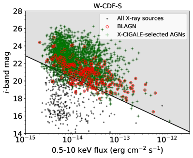
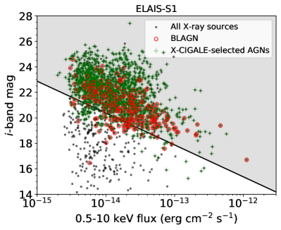
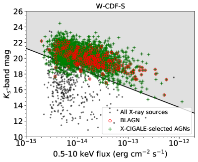
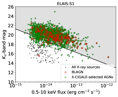
Figure 28: Left/Right: HSC (or DES) $i$-band/VIDEO $K_{s}$-band magnitude vs. X-ray flux in the full band for all the X-ray sources detected in the $i$/$K_{s}$-band (black dots), $i$/$K_{s}$-band detected broad-line AGNs (red circles), $i$/$K_{s}$-band detected X-ray sources that are classified as AGNs from X-CIGALE SED fitting (green pluses) in W-CDF-S (top panels) and ELAIS-S1 (bottom panels). The shaded region marks the “AGN region” defined by the $\log_{10}f_{x}/f_{i}>-1$ or $\log_{10}f_{x}/f_{K_{s}}>-1.2$ threshold (represented by the black solid line).

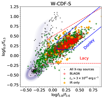
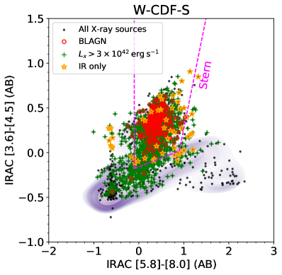
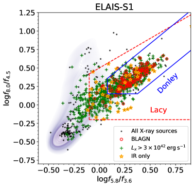
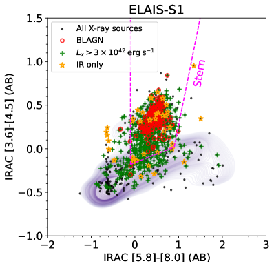
Figure 29: Left panels: The distribution of $\log f_{5.8}/f_{3.6}$ vs. $\log f_{8.0}/f_{4.5}$ for X-ray sources that are detected in four IRAC bands (black dots), with the 2D kernel-density plot of all SWIRE sources detected in four IRAC bands in the background in W-CDF-S (top) and ELAIS-S1 (bottom). Among these X-ray sources, broad-line AGNs are marked by the red circles; AGNs identified with high $L_{X}$ values are marked by green pluses; and X-ray sources that are only identified as AGN via MIR colors are marked by orange stars. The blue lines denote the Donley wedge (Donley et al., 2012); the red dashed lines denote the Lacy wedge (Lacy et al., 2004). Right panels: The distribution of IRAC$[5.8]-[8.0]$ vs. $[3.6]-[4.5]$ (AB) for all X-ray sources that are detected in four IRAC bands (black dots), with the 2D kernel-density plot of all SWIRE sources detected in four IRAC bands in the background in W-CDF-S (top) and ELAIS-S1 (bottom). Symbols represent the similar objects as the left panel. The magenta dashed lines denote the Stern wedge (Stern et al., 2005).

7 Summary and Future Work

We have presented the X-ray point-source catalogs for two of the XMM-SERVS fields, W-CDF-S and ELAIS-S1, in this work. These are the final two fields of the $\approx 30$ ks depth XMM-Newton survey, XMM-SERVS ($\approx 13~{}{\rm deg}^{2}$ in total). The main results are the following:

1. 2.3 Ms and 1.0 Ms of XMM-Newton observations were performed in the $\approx 4.6$ deg² W-CDF-S field and the $\approx 3.2$ deg² ELAIS-S1 field, respectively. After background filtering, the median cleaned PN+MOS1+MOS2 exposure time is $\approx 84$ ks in W-CDF-S and $\approx 80$ ks in ELAIS-S1 (see Section 2). Our survey in W-CDF-S/ELAIS-S1 has a flux limit of $1.0\times 10^{-14}$/ $1.3\times 10^{-14}$ erg cm^-2 s^-1 over 90% of its area in the 0.5–10 keV band (see Section 3.6).

2. We compiled the X-ray point-source catalogs in W-CDF-S and ELAIS-S1 with the SAS task emldetect. Adopting detection likelihoods that correspond to a spurious fraction of $\approx 1\%$ (obtained through simulations; see Section 3.3), 4053 point sources are detected in W-CDF-S, and 2630 point sources are detected in ELAIS-S1. These X-ray sources have a median positional uncertainty of $\approx 1.2$ arcsec (see Section 3).

3. Utilizing optical-to-NIR data from DES, HSC, VOICE, VIDEO, and DeepDrill, we use NWAY to identify multiwavelength counterparts for X-ray sources in the catalogs. 3600 ($\approx 89\%$) X-ray sources in W-CDF-S and 2288 ($\approx 87\%$) X-ray sources in ELAIS-S1 are matched to reliable optical and/or NIR counterparts (see Section 4).

4. Photometric redshifts are estimated for 3319/2001 X-ray sources in W-CDF-S/ELAIS-S1 with optical-to-NIR forced photometry available; type 1 AGNs are identified and fit separately with a suitable SED library. 2752 X-ray  sources in W-CDF-S and 1702 X-ray sources in ELAIS-S1 have either spectroscopic or high-quality ($\sigma_{\rm NMAD}\approx 0.03$–0.04 for non-BL AGNs and $\sigma_{\rm NMAD}\approx 0.06$–0.07 for BL AGNs when compared to spec-$z$s) photometric redshifts (see Section 5).

5. We identify 3186 X-ray sources in W-CDF-S and 1985 X-ray sources in ELAIS-S1 as AGNs based on their optical spectroscopic properties, X-ray luminosity and/or spectral shape, and X-ray-to-NIR SED template fitting results. MIR color and radio luminosity are also utilized to select AGNs when available (see Section 6).

The X-ray point-source catalogs provided in this work will have great legacy value for studies of AGNs across the full range of cosmic environments, and will enable large-scale studies of SMBH growth in the multi-dimensional space of galaxy parameters. We note that all the XMM-SERVS fields, including W-CDF-S and ELAIS-S1, are selected LSST deep-drilling fields, which will have $\approx 900$ epoch $ugrizy$ coverage with coadded depth reaching $i\approx 28$; the robustly identified X-ray AGNs will be useful for calibrating LSST AGN selection in the deep-drilling fields and the main survey. Future deep radio coverage from MIGHTEE (e.g., Jarvis et al., 2016), sub-millimeter coverage from LMT and ALMA, and spectroscopic data from DEVILS, MOONS, and WAVES (e.g., Davies et al., 2018; Driver et al., 2019; Maiolino et al., 2020) will also contribute to the legacy value of the W-CDF-S and ELAIS-S1 fields. The SDSS-V Black Hole Mapper Program (Kollmeier et al., 2017) and the 4MOST TiDES Program (Swann et al., 2019) will provide direct SMBH masses for hundreds of the AGNs in these fields. Together with this superior multiwavelength coverage, the X-ray catalogs presented in this work will enable outstanding studies of the $\approx$ 5200 AGNs reported. We leave detailed characterization of extended X-ray sources in the XMM-SERVS fields for future work, which will contribute to the studies of X-ray groups and clusters (e.g., Pierre et al., 2016).

Appendix A Main X-ray source catalog description

The descriptions of the columns included in our main X-ray source catalogs in W-CDF-S and ELAIS-S1 (see Tables 6 and 7) are presented below in a format similar to that of Chen et al. (2018). Throughout the table, null values are set to $-99$. All celestial coordinates are given in equinox J2000.

Table 6: The main X-ray source catalog in W-CDF-S with a selection of columns.

XID	RA	DEC	XPOSERR	FB_EXP	FB_BKG	FB_SCTS	0p5_10_FLUX	SPECZ	AGN_FLAG
(1)	(2)	(3)	(4)	(19)	(31)	(43)	(104)	(189)	(206)
WCDFS0000	52.152070	$-$28.698755	0.14	90110.6	3.78	8505.6	1.13635	0.10870	1
WCDFS0001	52.168228	$-$28.669922	0.29	118105.5	4.87	1948.1	0.05208	0.77247	1
WCDFS0002	52.130722	$-$28.880466	0.30	64600.6	3.95	1917.3	0.11816	1.04995	1
WCDFS0003	52.136161	$-$28.733398	0.33	100678.1	4.05	1555.2	0.04719	$-$99	1
WCDFS0004	51.876881	$-$28.512461	0.34	99457.5	3.23	1430.5	0.05912	0.38893	1
…	…	…	…	…	…	…	…	…	…

A detailed description of each column is presented in Appendix A. This table is available in its entirety in machine-readable form online.

Table 7: The main X-ray source catalog in ELAIS-S1 with a selection of columns.

XID	RA	DEC	XPOSERR	FB_EXP	FB_BKG	FB_SCTS	0p5_10_FLUX	SPECZ	AGN_FLAG
(1)	(2)	(3)	(4)	(19)	(31)	(43)	(104)	(180)	(197)
ES0000	8.747565	$-$44.824939	0.13	42850.9	1.96	5539.8	0.56817	-99.0	1
ES0001	8.726280	$-$44.771419	0.16	52141.0	2.00	3727.6	0.32483	0.40723	1
ES0002	9.324548	$-$44.503995	0.21	118323.1	5.71	2356.2	0.11067	1.32429	1
ES0003	9.087287	$-$44.144419	0.23	58336.4	2.29	2011.9	0.23091	0.20828	1
ES0004	8.787302	$-$44.310709	0.25	70255.8	1.81	1770.0	0.13339	0.34187	1
…	…	…	…	…	…	…	…	…	…

A detailed description of each column is presented in Appendix A. This table is available in its entirety in machine-readable form online.

Table 6: X-ray source catalog in W-CDF-S
X-ray properties
Columns 1–110 list the X-ray properties of our sources. Columns for the soft/hard/full-band results are marked with the “SB_”/“HB_”/“FB_” prefix.

• Column 1, XID: The source ID of each X-ray source.

• Columns 2–3, RA, DEC: RA and DEC (in degrees) of the X-ray source. Based on availability, we use the positions from, in priority order, the full band, soft band, and hard band as the primary position. Band-specific positions are listed in Columns 8–13.

• Column 4, XPOSERR: X-ray positional uncertainty ($\sigma_{x}$) in arcsec (reported with the same priority order as that of positions).

• Columns 5–6, R68, R99: 68% and 99.73% X-ray positional uncertainties in arcsec based on the Rayleigh distribution (see Section 3.4).

• Column 7, EMLERR: Positional uncertainties calculated by emldetect, $\sigma_{\rm eml}$, in arcsec (with the same priority order as that of positions).

• Columns 8–13, SB_RA, SB_DEC, HB_RA, HB_DEC, FB_RA, FB_DEC: RA and DEC (in degrees) of the source in the soft, hard, and full bands, respectively.

• Columns 14–16, SB_DET_ML, HB_DET_ML, FB_DET_ML: The emldetect source-detection likelihood in each band.

• Columns 17–19, SB_EXP, HB_EXP, FB_EXP: Total (PN + MOS1 + MOS2) exposure time in seconds in each band.

• Columns 20–28, SB_EXPPN, SB_EXPM1, SB_EXPM2, HB_EXPPN, HB_EXPM1, HB_EXPM2, FB_EXPPN, FB_EXPM1, FB_EXPM2: PN, MOS1, and MOS2 exposure times in seconds in each band.

• Columns 29–31, SB_BKG, HB_BKG, FB_BKG: Total background-map values (PN + MOS1 + MOS2) in counts per pixel in each band.

• Columns 32–40, SB_BKGPN, SB_BKGM1, SB_BKGM2, HB_BKGPN, HB_BKGM1, HB_BKGM2, FB_BKGPN, FB_BKGM1, FB_BKGM2: PN, MOS1, and MOS2 background-map values in counts per pixel in each band.

• Columns 41–43, SB_SCTS, HB_SCTS, FB_SCTS: Total (PN + MOS1 + MOS2) net counts in each band.

• Columns 44–52, SB_SCTSPN, SB_SCTSM1, SB_SCTSM2, HB_SCTSPN, HB_SCTSM1, HB_SCTSM2, FB_SCTSPN, FB_SCTSM1, FB_SCTSM2: PN, MOS1, and MOS2 net counts in each band.

• Columns 53–64, SB_SCTS_ERR, HB_SCTS_ERR, FB_SCTS_ERR, SB_SCTSPN_ERR, SB_SCTSM1_ERR, SB_SCTSM2_ERR, HB_SCTSPN_ERR, HB_SCTSM1_ERR, HB_SCTSM2_ERR, FB_SCTSPN_ERR, FB_SCTSM1_ERR, FB_SCTSM2_ERR: Uncertainties of total, PN, MOS1, and MOS2 net counts in each band reported in emldetect.

• Columns 65–76, SB_RATE, HB_RATE, FB_RATE, SB_RATEPN, SB_RATEM1, SB_RATEM2, HB_RATEPN, HB_RATEM1, HB_RATEM2, FB_RATEPN, FB_RATEM1, FB_RATEM2: Total, PN, MOS1, and MOS2 net count rates in each band, in count s^-1.

• Columns 77–88, SB_RATE_ERR, HB_RATE_ERR, FB_RATE_ERR, SB_RATEPN_ERR, SB_RATEM1_ERR, SB_RATEM2_ERR, HB_RATEPN_ERR, HB_RATEM1_ERR, HB_RATEM2_ERR, FB_RATEPN_ERR, FB_RATEM1_ERR, FB_RATEM2_ERR: Uncertainties of total, PN, MOS1, and MOS2 net count rates in each band, in count s^-1.

• Column 89–96, BR, BR_ERR, BRPN, BRPN_ERR, BRM1, BRM1_ERR, BRM2, BRM2_ERR: Total hard-to-soft band ratio and its uncertainty, and the hard-to-soft band ratio and its uncertainty for each EPIC detector.

• Column 97–98, HR, HR_ERR: Hardness ratio and its uncertainty.

• Column 99, GAMMA: The effective power-law photon index, $\Gamma_{\rm eff}$, derived for each source based on the hard-to-soft band ratio.

• Columns 100–105, 0p5_2_FLUX, 0p5_2_FLUX_ERR, 2_10_FLUX, 2_10_FLUX_ERR, 0p5_10_FLUX, 0p5_10_FLUX_ERR: Observed flux and flux uncertainty in the 0.5–2, 2–10, and 0.5–10 keV bands, in $10^{-12}$ erg cm^-2 s^-1, after correcting for Galactic absorption. The fluxes and uncertainties reported here are the error-weighted average of all EPIC detectors.

• Column 106, LX: Logarithm of rest-frame observed 2–10 keV X-ray luminosity (in erg s^-1) after correcting for Galactic absorption.

• Column 107, CHANDRA_SOURCE: The catalog origin of the nearest Chandra source within 10^′′. An entry of “1” stands for the CDF-S catalog (Luo et al., 2017), “2” stands for the E-CDF-S catalog (Xue et al., 2016), and “3” stands for the CSC 2.0 catalog.

• Column 108, CHANDRA_ID: Chandra source ID.

• Column 109–110, CHANDRA_RA, CHANDRA_DEC: RA and DEC (in degrees) of the matched Chandra counterpart.

Multiwavelength properties
Columns 111–207 provide the multiwavelength properties of the matched counterparts with match_flag $=1$ utilizing NWAY.

• Column 111, P_ANY: The posterior probability of the X-ray source having any correct counterparts ($p_{\rm any}$).

• Column 112, P_I: The relative probability ($p\_i$) of the reported match_flag $=1$ counterpart to be the correct match.

• Column 113, FLAG_SECOND: Warning flag for sources where a second possible counterpart is indicated by NWAY.

• Columns 114–121, IRAC_RA, IRAC_DEC, VIDEO_RA, VIDEO_DEC, HSC_RA, HSC_DEC, DES_RA, DES_DEC: RA and DEC of the counterpart in the DeepDrill/VIDEO/HSC/DES catalog in degrees. Note that DES counterparts are only reported in areas lacking HSC coverage.

• Columns 122–125, SEP_IRAC, SEP_VIDEO, SEP_HSC, SEP_DES: Separation of the X-ray position from the DeepDrill/VIDEO/HSC/DES counterpart in arcseconds.

• Columns 126–129, IRAC_1_MAG, IRAC_1_MAG_ERR, IRAC_2_MAG, IRAC_2_MAG_ERR: $1.9^{\prime\prime}$ aperture photometry and uncertainties in the IRAC $3.6\mu$m and $4.5\mu$m bands reported in the DeepDrill catalog.

• Columns 130–139, VIDEO_Z_MAG, VIDEO_Z_MAG_ERR, VIDEO_Y_MAG, VIDEO_Y_MAG_ERR, VIDEO_J_MAG, VIDEO_J_MAG_ERR, VIDEO_H_MAG, VIDEO_H_MAG_ERR, VIDEO_KS_MAG, VIDEO_KS_MAG_ERR: VIDEO 2^′′ aperture photometry and uncertainties in the $Z$, $Y$, $J$, $H$, and $K_{s}$ bands.

• Columns 140–147, HSC_G_MAG, HSC_G_MAG_ERR, HSC_R_MAG, HSC_R_MAG_ERR, HSC_I_MAG, HSC_I_MAG_ERR, HSC_Z_MAG, HSC_Z_MAG_ERR: HSC CModel photometry and uncertainties in the $g$, $r$, $i$, and $z$ bands.

• Columns 148–157, DES_G_MAG, DES_G_MAG_ERR, DES_R_MAG, DES_R_MAG_ERR, DES_I_MAG, DES_I_MAG_ERR, DES_Z_MAG, DES_Z_MAG_ERR, DES_Y_MAG, DES_Y_MAG_ERR: DES Kron Magnitude and uncertainties in the $g$, $r$, $i$, $z$, and $Y$ bands.

• Column 158, TRACTOR_ID: The object ID of the VIDEO counterpart in the forced-photometry catalog (Nyland et al. 2021).

• Columns 159–188, IRAC_1_FP_MAG, IRAC_1_FP_MAG_ERR, IRAC_2_FP_MAG, IRAC_2_FP_MAG_ERR, VIDEO_Z_FP_MAG, VIDEO_Z_FP_MAG_ERR, VIDEO_Y_FP_MAG,VIDEO_Y_FP_MAG_ERR, VIDEO_J_FP_MAG, VIDEO_J_FP_MAG_ERR, VIDEO_H_FP_MAG, VIDEO_H_FP_MAG_ERR, VIDEO_KS_FP_MAG, VIDEO_KS_FP_MAG_ERR, HSC_G_FP_MAG, HSC_G_FP_MAG_ERR, HSC_R_FP_MAG, HSC_R_FP_MAG_ERR, HSC_I_FP_MAG, HSC_I_FP_MAG_ERR, HSC_Z_FP_MAG, HSC_Z_FP_MAG_ERR, VOICE_U_FP_MAG, VOICE_U_FP_MAG_ERR, VOICE_G_FP_MAG,
  VOICE_G_FP_MAG_ERR, VOICE_R_FP_MAG, VOICE_R_FP_MAG_ERR, VOICE_I_FP_MAG, VOICE_I_FP_MAG_ERR: Forced photometry and uncertainties of DeepDrill $3.6\mu$m and $4.5\mu$m bands, VIDEO $ZYJHK_{s}$ bands, HSC $griz$ bands, and VOICE $ugri$ bands reported in the forced-photometry catalog (Nyland et al. 2021).

• Column 189, SPECZ: Spectroscopic redshift adopted for the X-ray source.

• Column 190, SPECZ_CLASS: Spectroscopic classification of the source. “1” stands for BL AGNs; “0” stands for galaxies or non-BL AGNs; “$-1$” stands for stars.

• Column 191, SPECZ_Q: Spectroscopic quality flag of the source reported in the original catalog.

• Columns 192–193, SPECZ_RA, SPECZ_DEC: RA and DEC (in degrees) of the spec-$z$.

• Column 194, SPECZ_SOURCE: The spectroscopic catalog listed in Table 5 that provides the spec-$z$.

• Column 195, SED_BLAGN_FLAG: Flag for BL AGN candidates identified in Appendix B. An entry of “1” stands for sources that are classified as BL AGN candidates by two different methods; “0.5” stands for sources identified as BL AGN candidates using one method but not the other; “0” indicates sources identified as non-BL AGNs by both methods.

• Columns 196–197, PHOTOZ_RA, PHOTOZ_DEC: RA and DEC (in degrees) of the source in the forced-photometry catalog (Nyland et al. in 2021), which includes forced photometry from DeepDrill, VIDEO, HSC, and VOICE that is utilized to compute photo-$z$s.

• Column 198, PHOTOZ_BEST: Photometric redshift adopted for the source. PHOTOZ_EAZY values are adopted for sources that have SED_BLAGN_FLAG $<$ 1 and are not identified as BL AGNs in spectroscopic surveys, when PHOTOZ_EAZY_Q $<1$; PHOTOZ_LEPHARE values are adopted for spectroscopically identified BL AGNs, SED_BLAGN_FLAG = 1 objects, and SED_BLAGN_FLAG $=0.5$ objects with PHOTOZ_EAZY_Q $\geqslant 1$ (see Section 5.2 for details).

• Columns 199–202, PHOTOZ_EAZY, PHOTOZ_EAZY_UERR, PHOTOZ_EAZY_LERR, PHOTOZ_EAZY_Q: Photometric redshift computed by EAZY, the associated upper and lower uncertainties, and the photometric-redshift quality parameter ($Q_{z}$).

• Columns 203–205, PHOTOZ_LEPHARE, PHOTOZ_LEPHARE_UERR, PHOTOZ_LEPHARE_LERR: Photometric redshift computed by LePhare and the associated upper and lower uncertainties. We only report LePhare photo-$z$s with $\chi_{\rm red}^{2}<2$ and band number $>10$ (see Section 5.2 for details).

• Column 206, AGN_FLAG: Flag for AGNs identified in Section 6.

• Column 207, STAR_FLAG: Flag for stars identified in Appendix C.

Table 7: X-ray source catalog in ELAIS-S1
X-ray properties
Columns 1–110 give the X-ray properties of our sources in the same format as that of Table  6.

Multiwavelength properties
Columns 111–198 provide the multiwavelength properties of the matched counterparts with match_flag $=1$ utilizing NWAY.

• Columns 111–113, P_ANY, P_I, FLAG_SECOND: see Columns 111–113 of Table 6.

• Columns 114–119, IRAC_RA, IRAC_DEC, VIDEO_RA, VIDEO_DEC, DES_RA, DES_DEC: RA and DEC of the counterpart in the DeepDrill/VIDEO/DES catalog in degrees.

• Columns 120–122, SEP_IRAC, SEP_VIDEO, SEP_DES: Separation of the X-ray position from the DeepDrill/VIDEO/DES counterpart in arcseconds.

• Columns 123–126, IRAC_1_MAG, IRAC_1_MAG_ERR, IRAC_2_MAG, IRAC_2_MAG_ERR: $1.9^{\prime\prime}$ aperture photometry and uncertainties in the IRAC $3.6\mu$m and $4.5\mu$m bands reported in the DeepDrill catalog.

• Columns 127–136, VIDEO_Z_MAG, VIDEO_Z_MAG_ERR, VIDEO_Y_MAG, VIDEO_Y_MAG_ERR, VIDEO_J_MAG, VIDEO_J_MAG_ERR, VIDEO_H_MAG, VIDEO_H_MAG_ERR, VIDEO_KS_MAG, VIDEO_KS_MAG_ERR: VIDEO 2^′′ aperture photometry and uncertainties in the $Z$, $Y$, $J$, $H$, and $K_{s}$ bands.

• Columns 137–146, DES_G_MAG, DES_G_MAG_ERR, DES_R_MAG, DES_R_MAG_ERR, DES_I_MAG, DES_I_MAG_ERR, DES_Z_MAG, DES_Z_MAG_ERR, DES_Y_MAG, DES_Y_MAG_ERR: DES Kron Magnitude and uncertainties in the $g$, $r$, $i$, $z$, and $Y$ bands.

• Column 147, TRACTOR_ID: The object ID of the VIDEO counterpart in the forced-photometry catalog (Zou et al., 2021).

• Columns 148–179, IRAC_1_FP_MAG, IRAC_1_FP_MAG_ERR, IRAC_2_FP_MAG, IRAC_2_FP_MAG_ERR, VIDEO_Z_FP_MAG, VIDEO_Z_FP_MAG_ERR, VIDEO_Y_FP_MAG, VIDEO_Y_FP_MAG_ERR, VIDEO_J_FP_MAG, VIDEO_J_FP_MAG_ERR, VIDEO_H_FP_MAG, VIDEO_H_FP_MAG_ERR, VIDEO_KS_FP_MAG, VIDEO_KS_FP_MAG_ERR, DES_G_FP_MAG, DES_G_FP_MAG_ERR, DES_R_FP_MAG, DES_R_FP_MAG_ERR, DES_I_FP_MAG, DES_I_FP_MAG_ERR, DES_Z_FP_MAG, DES_Z_FP_MAG_ERR, DES_Y_FP_MAG, DES_Y_FP_MAG_ERR, ESIS_B_FP_MAG,
  ESIS_B_FP_MAG_ERR, ESIS_V_FP_MAG, ESIS_V_FP_MAG_ERR, ESIS_R_FP_MAG, ESIS_R_FP_MAG_ERR, VOICE_U_FP_MAG, VOICE_U_FP_MAG_ERR: Forced photometry and uncertainties of DeepDrill $3.6\mu$m and $4.5\mu$m bands, VIDEO $ZYJHK_{s}$ bands, DES $grizY$ bands, ESIS $BVR$ bands, and VOICE $u$ band reported in the forced-photometry catalog (Zou et al., 2021).

• Columns 180–198, SPECZ, SPECZ_CLASS, SPECZ_Q, SPECZ_RA, SPECZ_DEC, SPECZ_SOURCE, SED_BLAGN_FLAG, PHOTOZ_RA, PHOTOZ_DEC, PHOTOZ_BEST, PHOTOZ_EAZY,PHOTOZ_EAZY_UERR, PHOTOZ_EAZY_LERR, PHOTOZ_EAZY_Q, PHOTOZ_LEPHARE, PHOTOZ_LEPHARE_UERR, PHOTOZ_LEPHARE_LERR, AGN_FLAG, STAR_FLAG: See Columns 188–206 of Table 6.

Appendix B Identifying BL AGN candidates

Considering its X-ray sensitivity limit, the XMM-SERVS survey would be able to detect $\approx 95\%$ of the spectroscopically identified BL AGNs in the COSMOS field (e.g., Marchesi et al., 2016), which is a survey field with rich spectroscopic observations. As the sky density of spectroscopically confirmed BL AGNs ($\approx 60$ deg^-2 for both W-CDF-S and ELAIS-S1) in our study is much less than that of COSMOS ($\approx 290$ deg^-2; Marchesi et al. 2016), we also identify BL AGN candidates in our X-ray catalogs that do not have spectroscopic classifications utilizing their SEDs via two independent methods: one method is based on machine learning, and the other is based on SED template fitting. As each of these methods has its own advantages and disadvantages, combining the results from both methods provides more reliable predictions for AGNs in our catalogs.

B.1 Machine-learning-based classification

For X-ray sources in W-CDF-S and ELAIS-S1 that have both spectroscopic classifications and forced photometry, we use machine learning to assess the differences between the optical-to-IR SEDs of X-ray sources that are classified as BL AGNs (260 in W-CDF-S and 179 in ELAIS-S1) and X-ray sources that are not BL AGNs (470 in W-CDF-S and 333 in ELAIS-S1). Utilizing all the available photometric data points, we normalized the SEDs so that all the data points have a maximum value of 0 in log space, and use the interp1d function in scipy to interpolate the log-space SED shape. We extract 16 data points at common observed-frame wavelengths from the interpolated SEDs (see Figure 30) to feed a 1D convolutional neutral network (CNN). Approximately $60\%$ of the objects are used as the training set; $\approx 20\%$ of the objects are used as the validation set; the remaining $\approx 20\%$ of the objects are used as the test set. After training the network and selecting the best model utilizing the validation set, we could correctly predict $\approx 86\%$ of the BL AGNs in the test set and $\approx 91\%$ of the sources that are not BL AGNs in W-CDF-S (see panel (a) of Figure 31 for the confusion matrix). When we apply the trained model to the remaining X-ray sources in the W-CDF-S forced-photometry catalog with signal-to-noise ratio (SNR) ¿ 3 detections in more than 5 bands, $\approx 790$ ($\approx 30\%$) of the sources are classified as BL AGN candidates. Combining these objects with the spectroscopically identified BL AGNs, the BL AGN density reaches $\approx 230$ deg^-2. Considering that only $\approx 80\%$ of the detected X-ray sources in W-CDF-S have reliably matched counterparts in the forced-photometry catalog (Nyland et al. 2021) with SNR ¿ 3 detections in more than 5 bands, this number is roughly consistent with the expectation from the COSMOS field. Similarly, after training the network in ELAIS-S1, we could correctly predict $\approx 80\%$ of the BL AGNs and $\approx 85\%$ of the sources that are not BL AGNs (see panel (c) of Figure 31). About $450$ ($\approx 30\%$) of the remaining X-ray sources in the ELAIS-S1 forced-photometry catalog with SNR ¿ 3 detections in more than 5 bands are classified as BL AGN candidates. The BL AGN density reaches $\approx 200$ deg^-2. Considering that only $\approx 70\%$ of the X-ray sources detected in ELAIS-S1 have SNR ¿ 3 detections in more than 5 bands in the Zou et al. (2021) forced-photometry catalog (while this number is 80% for W-CDF-S), this relatively low BL AGN density is also acceptable.

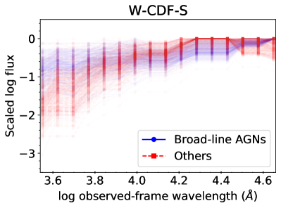
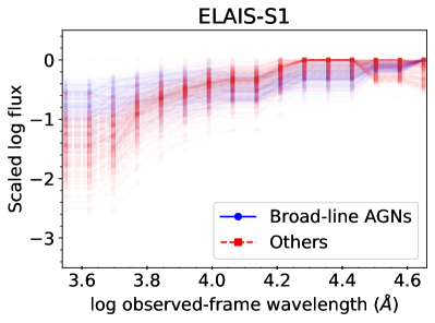
Figure 30: Extracted data points from the interpolated SEDs of broad-line AGNs identified in spectroscopic surveys (blue) compared with other X-ray sources that have spectroscopic classifications (red) in W-CDF-S (left) and ELAIS-S1 (right).

Figure 31: (a). The confusion matrix for the machine-learning based classification of X-ray sources in W-CDF-S. (b). The confusion matrix for the X-CIGALE-based classification of X-ray sources in W-CDF-S. (c). The confusion matrix for the machine-learning based classification of X-ray sources in ELAIS-S1. (d). The confusion matrix for the X-CIGALE-based classification of X-ray sources in ELAIS-S1.

B.2 SED-template-fitting-based classification

We also utilize X-CIGALE (Yang et al., 2020) to identify BL AGNs from their optical-to-IR SEDs in combination with the X-ray flux level. We do not provide redshift information to X-CIGALE, and allow X-CIGALE fit redshift as a free parameter. We adopt a delayed exponentially declining star formation history, a Chabrier initial mass function (Chabrier, 2003), the extinction law from Calzetti et al. (2000), the dust-emission template from Dale et al. (2014), the AGN component SKIRTOR (that is established based on Stalevski et al. 2012, 2016), and the X-ray module following Yang et al. (2020). Details of the fitting parameters are given in Table 8. As X-CIGALE requires intrinsic X-ray fluxes, we convert the observed X-ray flux derived in Section 3.5 to intrinsic absorption-corrected X-ray flux following the method in Section 4.4 of Luo et al. (2017). Basically, we assume that all X-ray sources with $\Gamma_{\rm eff}<1.8$ suffer from some level of intrinsic absorption, and their intrinsic spectra have power-law shapes with a fixed photon index of 1.8. To identify AGNs, we utilized the ratio between the Bayesian estimation of the AGN 2–10 keV luminosity and the sum of the Bayesian estimation of the 2–10 keV LMXB luminosity and HMXB luminosity in the X-CIGALE output: if this ratio is greater than 10, we identify the source as an AGN. As BL AGNs generally do not suffer from high levels of extinction of the AGN emission, if the Bayesian estimation for the $E(B-V)$ parameter of the AGN component is smaller than 0.2, we classify the AGN as a BL AGN candidate. We tested the accuracy of the template-fitting-based classification utilizing X-ray sources that have spectroscopic classifications available; the confusion matrix can be seen in the relevant panels of Figure 31. We correctly predict $\approx 78\%$ of the BL AGNs and $\approx 83\%$ of the sources that are not BL AGNs in W-CDF-S; we correctly predict $\approx 70\%$ of the BL AGNs and $\approx 86\%$ of the sources that are not BL AGNs in ELAIS-S1. When we fit the remaining X-ray sources in the forced-photometry catalog that do not have spectroscopic classifications available, $\approx 690$/350 of the sources in W-CDF-S/ELAIS-S1 are classified as BL AGN candidates. As template fitting strongly relies on the number of photometric points available, the resulting BL AGN sky density ($\approx 210/180$ deg^-2 in W-CDF-S/ELAIS-S1) is roughly consistent with the expectation from the COSMOS field: only $\approx 65\%$ of the X-ray sources in W-CDF-S and ELAIS-S1 without spectroscopic redshifts have SNR ¿ 3 detections in at least 10 bands.

Table 8: Utilized X-CIGALE modules with fitting parameters. Default values are adopted for parameters not listed.

Module	Parameters	Values
Star formation history: sfhdelayed	$\tau$ (Myr)	100, 300, 500, 1000, 5000, 8000
	$t$ (Myr)	100, 300, 500, 1000, 2000, 3000, 5000, 7000, 10000
Stellar population synthesis model: bc03	Initial mass function	Chabrier (2003)
Dust attenuation: dustatt_calzetti	$E(B-V)$	0.2–1.0 with steps of 0.1
Dust emission: dale2014	$\alpha$ in d$M_{\rm dust}\propto U^{-\alpha}{\rm d}U$	2.0
AGN emission: skirtor2016	Torus optical depth at 9.7$\mu$m	7
	Viewing angle (∘)	30
	AGN fraction of total IR luminosity ($\rm frac_{AGN}$)	0–0.9 with steps of 0.1, and 0.99
	$E(B-V)$ of AGN polar dust	0–0.6 with steps of 0.1
X-ray	$\Gamma$	1.8
	max$|\Delta\alpha_{\rm OX}|$	0.2

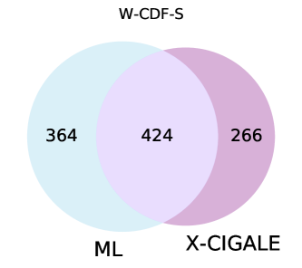
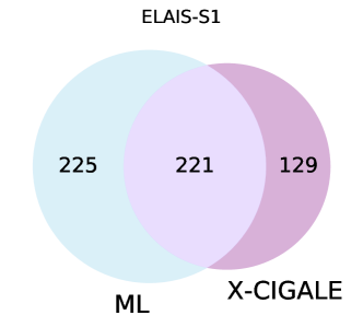
Figure 32: The Venn diagram for BL AGNs identified with the machine-learning-based approach and the X-CIGALE template-fitting-based approach.

B.3 Assessing the reliability of BL AGN candidates identified

The above two methods each have advantages and disadvantages. The machine-learning-based method achieves a higher apparent level of accuracy; at the same time, as the model is trained based upon BL AGNs with spectroscopic classifications (which are brighter compared with sources not identified in spectroscopic surveys), there might be biases associated with the predictions. While the template-fitting-based method does not suffer from the potential bias introduced from the training set, its accuracy is lower. Also, for both methods, the prediction accuracy declines when the available number of photometric data points is smaller. Thus, we create a flag, SED_BLAGN_FLAG, for the BL AGN candidates identified. SED_BLAGN_FLAG $=1$ is assigned to $\approx 420$/220 X-ray sources in W-CDF-S/ELAIS-S1 that are identified as BL AGN candidates by both methods; SED_BLAGN_FLAG $=0.5$ is assigned to $\approx 630$/350 X-ray sources in W-CDF-S/ELAIS-S1 that are identified as BL AGN candidates with one method but not the other (see Figure 32 for the Venn diagram).

To assess the reliability of the BL AGN candidates identified, we check the morphology and optical variability of BL AGN candidates identified in W-CDF-S. As luminous BL AGNs often appear to be point-like sources when they dominate over host-galaxy starlight, morphological information has been adopted in selecting BL AGN candidates in some literature works (e.g., Salvato et al., 2009, 2011). In the HSC catalog presented in Ni et al. (2019), the sdss_pointlike flag selects point-like sources with the SDSS algorithm, psfMag - CmodelMag ¡ 0.145, in the reference band (the band in which the source is detected with the highest SNR). Utilizing this sdss_pointlike column, 1346 X-ray sources in W-CDF-S are considered to be point-like through HSC morphology. Among 731 X-ray sources where spectroscopic classifications are available, HSC morphology could correctly classify $\approx 93\%$ of the BL AGNs and $\approx 82\%$ of the sources that are not BL AGNs. However, as HSC morphology becomes less accurate at higher redshift and fainter magnitudes, we only utilize it to assess the reliability of objects marked with SED_BLAGN_FLAG $=1$ or $=0.5$: although not all point-like sources identified from HSC morphology are BL AGNs, we do expect a substantial fraction of the BL AGNs identified via SEDs to have sdss_pointlike $=1$. Figure 33 shows that $\approx 64\%$ of the X-ray sources marked with SED_BLAGN_FLAG $=1$ or $=0.5$ in W-CDF-S are identified as point-like sources utilizing HSC morphology. This fraction is $\approx 87\%$ for SED_BLAGN_FLAG $=1$ sources, and $\approx 48\%$ for SED_BLAGN_FLAG $=0.5$ sources, suggesting that SED_BLAGN_FLAG $=1$ is more reliable in identifying BL AGNs, as expected.

The catalogs of optically variable sources in W-CDF-S from Falocco et al. (2015) and Poulain et al. (2020) are also utilized to assess the quality of the BL AGN candidates selected from SEDs. 333 of our X-ray sources in W-CDF-S are identified as potential AGNs in these catalogs (class $\geqslant$ 0), and these sources are likely to be BL AGNs. Approximately 160 of them have spectroscopic classification: $\approx 70\%$ of them are real BL AGNs. Although the sample of BL AGN candidates identified via optical variability is incomplete and may have contamination (e.g., from supernovae or stars whose observed fluxes vary due to internal or external reasons), it remains a useful sample for testing the completeness of BL AGNs identified via SEDs. As can be seen in Figure 33, SED_BLAGN_FLAG $=1$ or $=0.5$ objects in W-CDF-S include $\approx 81\%$ of the optically variable sources; SED_BLAGN_FLAG $=1$ objects alone only include $\approx 58\%$ of the optically variable sources. Thus, the utilization of SED_BLAGN_FLAG $=1$ alone will likely lead to a relatively incomplete BL AGN identification.

For the purposes of this work, we would like to provide reliable photo-$z$ estimations for X-ray sources. About $70\%$/$60\%$ of the SED_BLAGN_FLAG $=1/0.5$ objects in W-CDF-S and ELAIS-S1 do not have high-quality ($Q_{z}<1$) EAZY photo-$z$ measurements utilizing galaxy and obscured AGN templates (see Section 5.2). Thus, we use the AGN-dominated SED templates to fit all the SED_BLAGN_FLAG $=1$ objects, and all the SED_BLAGN_FLAG $=0.5$ sources that cannot be characterized well (i.e., with $Q_{z}<1$) by galaxy/obscured AGN templates (see Section 5.2).

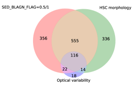
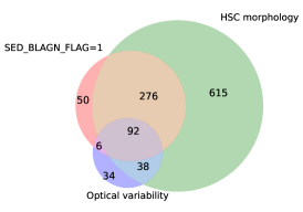
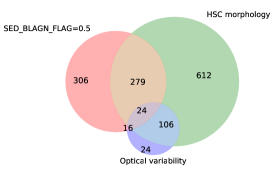
Figure 33: Left: The Venn diagram for the SED_BLAGN_FLAG $=1$ or 0.5 sources, point-like sources identified via HSC morphology, and reported optically variable sources in the W-CDF-S field. Middle: Similar to the left panel, but for the SED_BLAGN_FLAG $=1$ sources. Right: Similar to the left panel, but for the SED_BLAGN_FLAG $=0.5$ sources.

Appendix C Identifying non-AGN X-ray sources

We have identified Galactic stars among non-AGN X-ray sources that are associated with reliable multiwavelength counterparts (see Section 6) based on the $g-z$ (or $B-z$) vs. $z-K_{s}$ diagram in W-CDF-S (or ELAIS-S1); sources falling below the dashed line in Figure 34 are classified as stars. Figure 34 demonstrates that this criterion successfully identifies almost all of the spectroscopically-confirmed stars. We also match the non-AGN X-ray sources to Gaia sources (e.g., Gaia Collaboration et al., 2018) with a matching radius of 1^′′, and classify sources with significant proper motions as stars. We visually examined the optical imaging to remove contaminating galaxies with obviously extended morphology. In total, 163 out of the 429 non-AGN X-ray sources in W-CDF-S are classified as stars; 89 out of the 317 non-AGN X-ray sources in ELAIS-S1 are classified as stars. For the remaining non-AGN X-ray sources, most are bright and large foreground galaxies (identified via visual examination) that contain a population of X-ray binaries and/or a low-luminosity AGN (see Figure 35 for example cutouts).

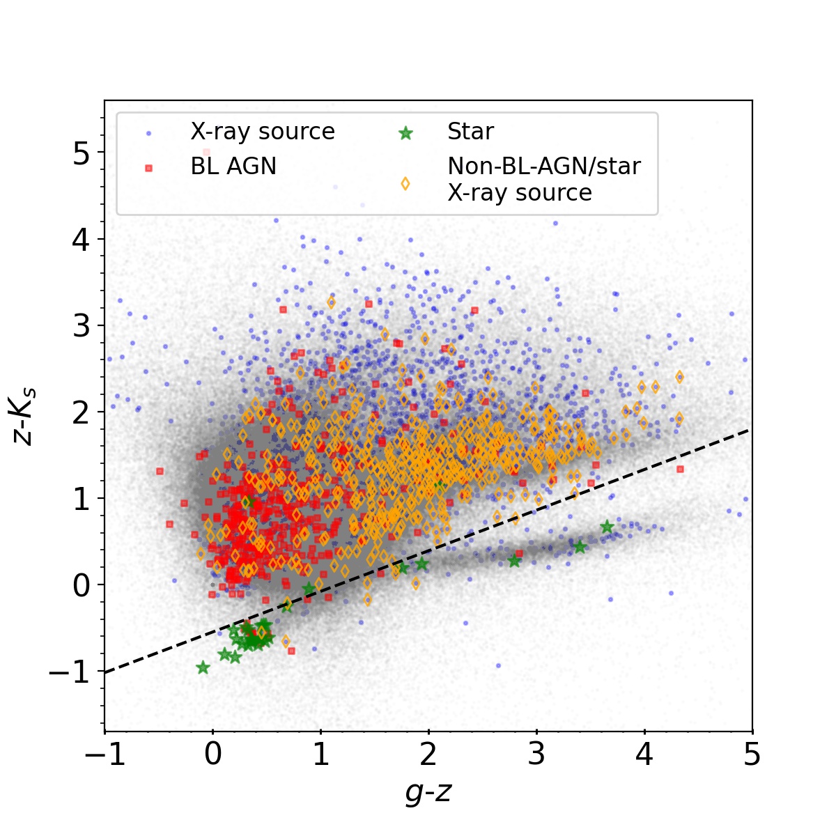
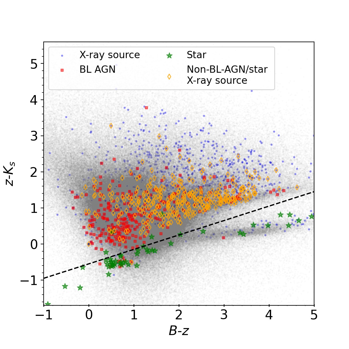
Figure 34: Left: The $g-z$ vs. $z-K_{s}$ diagram for sources in the W-CDF-S forced-photometry catalog (Nyland et al. 2021) represented by the grey dots, which can be utilized to separate stars from other X-ray sources. X-ray sources are marked as blue circles; spectroscopically confirmed BL AGNs are indicated by red squares; spectroscopically identified stars are marked as green stars; X-ray sources with spectroscopic classification that are not identified as BL AGNs nor stars are represented by orange diamonds. The black dashed line is utilized to identify stars among non-AGN sources. Right: The $B-z$ vs. $z-K_{s}$ diagram for sources in the ELAIS-S1 forced-photometry catalog (Zou et al., 2021). Symbols are similar to the top panel.

Figure 35: Example multiwavelength cutouts of X-ray detected stars (a/b) and X-ray detected galaxies (c/d) in W-CDF-S/ELAIS-S1. Each panel shows four $40^{\prime\prime}\times 40^{\prime\prime}$ cutouts: XMM-Newton 0.2–12 keV (top-left), DeepDrill 3.6$\mu$m band (top-right), VIDEO $K_{s}$-band (bottom-left), and HSC (or DES) $i$-band (bottom-right).

References

- Abazajian et al. (2009) Abazajian, K. N., Adelman-McCarthy, J. K., Agüeros, M. A., et al. 2009, ApJS, 182, 543, doi: 10.1088/0067-0049/182/2/543
- Abbott et al. (2021) Abbott, T. M. C., Adamow, M., Aguena, M., et al. 2021, arXiv e-prints, arXiv:2101.05765. https://arxiv.org/abs/2101.05765
- Aird et al. (2015) Aird, J., Coil, A. L., Georgakakis, A., et al. 2015, MNRAS, 451, 1892, doi: 10.1093/mnras/stv1062
- Alexander et al. (2005) Alexander, D. M., Bauer, F. E., Chapman, S. C., et al. 2005, ApJ, 632, 736, doi: 10.1086/444342
- Ananna et al. (2017) Ananna, T. T., Salvato, M., LaMassa, S., et al. 2017, ApJ, 850, 66, doi: 10.3847/1538-4357/aa937d
- Arnouts et al. (1999) Arnouts, S., Cristiani, S., Moscardini, L., et al. 1999, MNRAS, 310, 540, doi: 10.1046/j.1365-8711.1999.02978.x
- Berta et al. (2006) Berta, S., Rubele, S., Franceschini, A., et al. 2006, A&A, 451, 881, doi: 10.1051/0004-6361:20054548
- Brammer et al. (2008) Brammer, G. B., van Dokkum, P. G., & Coppi, P. 2008, ApJ, 686, 1503, doi: 10.1086/591786
- Brandt & Alexander (2015) Brandt, W. N., & Alexander, D. M. 2015, A&A Rev., 23, 1, doi: 10.1007/s00159-014-0081-z
- Brandt et al. (2018) Brandt, W. N., Ni, Q., Yang, G., et al. 2018, arXiv e-prints, arXiv:1811.06542. https://arxiv.org/abs/1811.06542
- Broos et al. (2011) Broos, P. S., Townsley, L. K., Feigelson, E. D., et al. 2011, ApJS, 194, 2, doi: 10.1088/0067-0049/194/1/2
- Calzetti et al. (2000) Calzetti, D., Armus, L., Bohlin, R. C., et al. 2000, ApJ, 533, 682, doi: 10.1086/308692
- Cappelluti et al. (2009) Cappelluti, N., Brusa, M., Hasinger, G., et al. 2009, A&A, 497, 635, doi: 10.1051/0004-6361/200810794
- Chabrier (2003) Chabrier, G. 2003, PASP, 115, 763, doi: 10.1086/376392
- Chen et al. (2018) Chen, C. T. J., Brandt, W. N., Luo, B., et al. 2018, MNRAS, 478, 2132, doi: 10.1093/mnras/sty1036
- Chiappetti et al. (2018) Chiappetti, L., Fotopoulou, S., Lidman, C., et al. 2018, A&A, 620, A12, doi: 10.1051/0004-6361/201731880
- Civano et al. (2016) Civano, F., Marchesi, S., Comastri, A., et al. 2016, ApJ, 819, 62, doi: 10.3847/0004-637X/819/1/62
- Coil et al. (2011) Coil, A. L., Blanton, M. R., Burles, S. M., et al. 2011, ApJ, 741, 8, doi: 10.1088/0004-637X/741/1/8
- Colless et al. (2001) Colless, M., Dalton, G., Maddox, S., et al. 2001, MNRAS, 328, 1039, doi: 10.1046/j.1365-8711.2001.04902.x
- Comastri et al. (2011) Comastri, A., Ranalli, P., Iwasawa, K., et al. 2011, A&A, 526, L9, doi: 10.1051/0004-6361/201016119
- Cooper et al. (2012) Cooper, M. C., Yan, R., Dickinson, M., et al. 2012, MNRAS, 425, 2116, doi: 10.1111/j.1365-2966.2012.21524.x
- Dale et al. (2014) Dale, D. A., Helou, G., Magdis, G. E., et al. 2014, ApJ, 784, 83, doi: 10.1088/0004-637X/784/1/83
- Davies et al. (2018) Davies, L. J. M., Robotham, A. S. G., Driver, S. P., et al. 2018, MNRAS, 480, 768, doi: 10.1093/mnras/sty1553
- Donley et al. (2005) Donley, J. L., Rieke, G. H., Rigby, J. R., & Pérez-González, P. G. 2005, ApJ, 634, 169, doi: 10.1086/491668
- Donley et al. (2012) Donley, J. L., Koekemoer, A. M., Brusa, M., et al. 2012, ApJ, 748, 142, doi: 10.1088/0004-637X/748/2/142
- Driver & Robotham (2010) Driver, S. P., & Robotham, A. S. G. 2010, MNRAS, 407, 2131, doi: 10.1111/j.1365-2966.2010.17028.x
- Driver et al. (2019) Driver, S. P., Liske, J., Davies, L. J. M., et al. 2019, The Messenger, 175, 46, doi: 10.18727/0722-6691/5126
- Eales et al. (2009) Eales, S., Chapin, E. L., Devlin, M. J., et al. 2009, ApJ, 707, 1779, doi: 10.1088/0004-637X/707/2/1779
- Evans et al. (2010) Evans, I. N., Primini, F. A., Glotfelty, K. J., et al. 2010, ApJS, 189, 37, doi: 10.1088/0067-0049/189/1/37
- Falocco et al. (2015) Falocco, S., Paolillo, M., Covone, G., et al. 2015, A&A, 579, A115, doi: 10.1051/0004-6361/201425111
- Feruglio et al. (2008) Feruglio, C., Fiore, F., La Franca, F., et al. 2008, A&A, 488, 417, doi: 10.1051/0004-6361:200809571
- Franzen et al. (2015) Franzen, T. M. O., Banfield, J. K., Hales, C. A., et al. 2015, MNRAS, 453, 4020, doi: 10.1093/mnras/stv1866
- Gaia Collaboration et al. (2018) Gaia Collaboration, Brown, A. G. A., Vallenari, A., et al. 2018, A&A, 616, A1, doi: 10.1051/0004-6361/201833051
- Ilbert et al. (2006) Ilbert, O., Arnouts, S., McCracken, H. J., et al. 2006, A&A, 457, 841, doi: 10.1051/0004-6361:20065138
- Jarvis et al. (2016) Jarvis, M., Taylor, R., Agudo, I., et al. 2016, in MeerKAT Science: On the Pathway to the SKA, 6. https://arxiv.org/abs/1709.01901
- Jarvis et al. (2013) Jarvis, M. J., Bonfield, D. G., Bruce, V. A., et al. 2013, MNRAS, 428, 1281, doi: 10.1093/mnras/sts118
- Jones et al. (2009) Jones, D. H., Read, M. A., Saunders, W., et al. 2009, MNRAS, 399, 683, doi: 10.1111/j.1365-2966.2009.15338.x
- Kelson et al. (2014) Kelson, D. D., Williams, R. J., Dressler, A., et al. 2014, ApJ, 783, 110, doi: 10.1088/0004-637X/783/2/110
- Kim et al. (2007) Kim, M., Wilkes, B. J., Kim, D.-W., et al. 2007, ApJ, 659, 29, doi: 10.1086/511630
- Klypin et al. (2016) Klypin, A., Yepes, G., Gottlöber, S., Prada, F., & Heß, S. 2016, MNRAS, 457, 4340, doi: 10.1093/mnras/stw248
- Kollmeier et al. (2017) Kollmeier, J. A., Zasowski, G., Rix, H.-W., et al. 2017, arXiv e-prints, arXiv:1711.03234. https://arxiv.org/abs/1711.03234
- Lacy et al. (2004) Lacy, M., Storrie-Lombardi, L. J., Sajina, A., et al. 2004, ApJS, 154, 166, doi: 10.1086/422816
- Lacy et al. (2021) Lacy, M., Surace, J. A., Farrah, D., et al. 2021, MNRAS, 501, 892, doi: 10.1093/mnras/staa3714
- LaMassa et al. (2019) LaMassa, S. M., Georgakakis, A., Vivek, M., et al. 2019, ApJ, 876, 50, doi: 10.3847/1538-4357/ab108b
- LaMassa et al. (2016) LaMassa, S. M., Urry, C. M., Cappelluti, N., et al. 2016, ApJ, 817, 172, doi: 10.3847/0004-637X/817/2/172
- Lang et al. (2016) Lang, D., Hogg, D. W., & Mykytyn, D. 2016, The Tractor: Probabilistic astronomical source detection and measurement. http://ascl.net/1604.008
- Lanzuisi et al. (2013) Lanzuisi, G., Civano, F., Elvis, M., et al. 2013, MNRAS, 431, 978, doi: 10.1093/mnras/stt222
- Levi et al. (2019) Levi, M., Allen, L. E., Raichoor, A., et al. 2019, in Bulletin of the American Astronomical Society, Vol. 51, 57. https://arxiv.org/abs/1907.10688
- Lidman et al. (2020) Lidman, C., Tucker, B. E., Davis, T. M., et al. 2020, MNRAS, 496, 19, doi: 10.1093/mnras/staa1341
- Liu et al. (2017) Liu, T., Tozzi, P., Wang, J.-X., et al. 2017, ApJS, 232, 8, doi: 10.3847/1538-4365/aa7847
- Liu et al. (2020) Liu, T., Merloni, A., Simm, T., et al. 2020, arXiv e-prints, arXiv:2009.02193. https://arxiv.org/abs/2009.02193
- Liu et al. (2016) Liu, Z., Merloni, A., Georgakakis, A., et al. 2016, MNRAS, 459, 1602, doi: 10.1093/mnras/stw753
- Lonsdale et al. (2003) Lonsdale, C. J., Smith, H. E., Rowan-Robinson, M., et al. 2003, PASP, 115, 897, doi: 10.1086/376850
- Luo et al. (2017) Luo, B., Brandt, W. N., Xue, Y. Q., et al. 2017, ApJS, 228, 2, doi: 10.3847/1538-4365/228/1/2
- Maiolino et al. (2020) Maiolino, R., Cirasuolo, M., Afonso, J., et al. 2020, The Messenger, 180, 24, doi: 10.18727/0722-6691/5197
- Mao et al. (2012) Mao, M. Y., Sharp, R., Norris, R. P., et al. 2012, MNRAS, 426, 3334, doi: 10.1111/j.1365-2966.2012.21913.x
- Marchesi et al. (2016) Marchesi, S., Civano, F., Elvis, M., et al. 2016, The Astrophysical Journal, 817, 34, doi: 10.3847/0004-637x/817/1/34
- Marshall et al. (1980) Marshall, F. E., Boldt, E. A., Holt, S. S., et al. 1980, ApJ, 235, 4, doi: 10.1086/157601
- Martin et al. (2005) Martin, D. C., Fanson, J., Schiminovich, D., et al. 2005, ApJ, 619, L1, doi: 10.1086/426387
- Mauduit et al. (2012) Mauduit, J. C., Lacy, M., Farrah, D., et al. 2012, PASP, 124, 714, doi: 10.1086/666945
- Menzel et al. (2016) Menzel, M. L., Merloni, A., Georgakakis, A., et al. 2016, MNRAS, 457, 110, doi: 10.1093/mnras/stv2749
- Monet et al. (2003) Monet, D. G., Levine, S. E., Canzian, B., et al. 2003, AJ, 125, 984, doi: 10.1086/345888
- Moster et al. (2011) Moster, B. P., Somerville, R. S., Newman, J. A., & Rix, H.-W. 2011, ApJ, 731, 113, doi: 10.1088/0004-637X/731/2/113
- Nandra et al. (2015) Nandra, K., Laird, E. S., Aird, J. A., et al. 2015, The Astrophysical Journal Supplement Series, 220, 10, doi: 10.1088/0067-0049/220/1/10
- Ni et al. (2019) Ni, Q., Timlin, J., Brandt, W. N., & Yang, G. 2019, Research Notes of the American Astronomical Society, 3, 5, doi: 10.3847/2515-5172/aaf8af
- Nyland et al. (2017) Nyland, K., Lacy, M., Sajina, A., et al. 2017, ApJS, 230, 9, doi: 10.3847/1538-4365/aa6fed
- Oliver et al. (2012) Oliver, S. J., Bock, J., Altieri, B., et al. 2012, MNRAS, 424, 1614, doi: 10.1111/j.1365-2966.2012.20912.x
- Pierre et al. (2016) Pierre, M., Pacaud, F., Adami, C., et al. 2016, A&A, 592, A1, doi: 10.1051/0004-6361/201526766
- Pineau et al. (2017) Pineau, F. X., Derriere, S., Motch, C., et al. 2017, A&A, 597, A89, doi: 10.1051/0004-6361/201629219
- Poulain et al. (2020) Poulain, M., Paolillo, M., De Cicco, D., et al. 2020, A&A, 634, A50, doi: 10.1051/0004-6361/201937108
- Puccetti et al. (2006) Puccetti, S., Fiore, F., D’Elia, V., et al. 2006, A&A, 457, 501, doi: 10.1051/0004-6361:20064904
- Ranalli et al. (2013) Ranalli, P., Comastri, A., Vignali, C., et al. 2013, A&A, 555, A42, doi: 10.1051/0004-6361/201321211
- Rosen et al. (2016) Rosen, S. R., Webb, N. A., Watson, M. G., et al. 2016, A&A, 590, A1, doi: 10.1051/0004-6361/201526416
- Sacchi et al. (2009) Sacchi, N., La Franca, F., Feruglio, C., et al. 2009, ApJ, 703, 1778, doi: 10.1088/0004-637X/703/2/1778
- Salvato et al. (2009) Salvato, M., Hasinger, G., Ilbert, O., et al. 2009, ApJ, 690, 1250, doi: 10.1088/0004-637X/690/2/1250
- Salvato et al. (2011) Salvato, M., Ilbert, O., Hasinger, G., et al. 2011, ApJ, 742, 61, doi: 10.1088/0004-637X/742/2/61
- Salvato et al. (2018) Salvato, M., Buchner, J., Budavári, T., et al. 2018, MNRAS, 473, 4937, doi: 10.1093/mnras/stx2651
- Scolnic et al. (2018) Scolnic, D. M., Lochner, M., Gris, P., et al. 2018, arXiv e-prints, arXiv:1812.00516. https://arxiv.org/abs/1812.00516
- Shirley et al. (2019) Shirley, R., Roehlly, Y., Hurley, P. D., et al. 2019, MNRAS, 490, 634, doi: 10.1093/mnras/stz2509
- Silverman et al. (2010) Silverman, J. D., Mainieri, V., Salvato, M., et al. 2010, ApJS, 191, 124, doi: 10.1088/0067-0049/191/1/124
- Skrutskie et al. (2006) Skrutskie, M. F., Cutri, R. M., Stiening, R., et al. 2006, AJ, 131, 1163, doi: 10.1086/498708
- Stalevski et al. (2012) Stalevski, M., Fritz, J., Baes, M., Nakos, T., & Popović, L. Č. 2012, MNRAS, 420, 2756, doi: 10.1111/j.1365-2966.2011.19775.x
- Stalevski et al. (2016) Stalevski, M., Ricci, C., Ueda, Y., et al. 2016, MNRAS, 458, 2288, doi: 10.1093/mnras/stw444
- Stern et al. (2005) Stern, D., Eisenhardt, P., Gorjian, V., et al. 2005, ApJ, 631, 163, doi: 10.1086/432523
- Swann et al. (2019) Swann, E., Sullivan, M., Carrick, J., et al. 2019, The Messenger, 175, 58, doi: 10.18727/0722-6691/5129
- Thorne et al. (2020) Thorne, J. E., Robotham, A. S. G., Davies, L. J. M., et al. 2020, arXiv e-prints, arXiv:2011.13605. https://arxiv.org/abs/2011.13605
- Traulsen et al. (2019) Traulsen, I., Schwope, A. D., Lamer, G., et al. 2019, A&A, 624, A77, doi: 10.1051/0004-6361/201833938
- Traulsen et al. (2020) —. 2020, A&A, 641, A137, doi: 10.1051/0004-6361/202037706
- Ueda et al. (2014) Ueda, Y., Akiyama, M., Hasinger, G., Miyaji, T., & Watson, M. G. 2014, ApJ, 786, 104, doi: 10.1088/0004-637X/786/2/104
- Ueda et al. (2008) Ueda, Y., Watson, M. G., Stewart, I. M., et al. 2008, ApJS, 179, 124, doi: 10.1086/591083
- Vaccari (2015) Vaccari, M. 2015, in Proceedings of “The many facets of extragalactic radio surveys: towards new scientific challenges” (EXTRA-RADSUR2015). 20-23 October 2015. Bologna, 27. https://arxiv.org/abs/1604.02353
- Vaccari et al. (2016) Vaccari, M., Covone, G., Radovich, M., et al. 2016, in The 4th Annual Conference on High Energy Astrophysics in Southern Africa (HEASA 2016), 26. https://arxiv.org/abs/1704.01495
- Vito et al. (2018) Vito, F., Brandt, W. N., Yang, G., et al. 2018, MNRAS, 473, 2378, doi: 10.1093/mnras/stx2486
- Webb et al. (2020) Webb, N. A., Coriat, M., Traulsen, I., et al. 2020, A&A, 641, A136, doi: 10.1051/0004-6361/201937353
- Willingale et al. (2013) Willingale, R., Starling, R. L. C., Beardmore, A. P., Tanvir, N. R., & O’Brien, P. T. 2013, MNRAS, 431, 394, doi: 10.1093/mnras/stt175
- Xue (2017) Xue, Y. Q. 2017, New A Rev., 79, 59, doi: 10.1016/j.newar.2017.09.002
- Xue et al. (2016) Xue, Y. Q., Luo, B., Brandt, W. N., et al. 2016, ApJS, 224, 15, doi: 10.3847/0067-0049/224/2/15
- Xue et al. (2011) —. 2011, ApJS, 195, 10, doi: 10.1088/0067-0049/195/1/10
- Yang et al. (2016) Yang, G., Brandt, W. N., Luo, B., et al. 2016, ApJ, 831, 145, doi: 10.3847/0004-637X/831/2/145
- Yang et al. (2018) Yang, G., Brandt, W. N., Vito, F., et al. 2018, MNRAS, 475, 1887, doi: 10.1093/mnras/stx2805
- Yang et al. (2020) Yang, G., Boquien, M., Buat, V., et al. 2020, MNRAS, 491, 740, doi: 10.1093/mnras/stz3001
- Zou et al. (2021) Zou, F., Brandt, W. N., Lacy, M., et al. 2021, Research Notes of the AAS, 5, 31, doi: 10.3847/2515-5172/abe769
- Zou et al. (2021) Zou, F., Yang, G., Brandt, W. N., et al. 2021, Research Notes of the American Astronomical Society, 5, 56, doi: 10.3847/2515-5172/abf050