ML and MAP Device Activity Detections for Grant-Free Massive Access in Multi-Cell Networks

Abstract

Device activity detection is one main challenge in grant-free massive access, which is recently proposed to support massive machine-type communications (mMTC). Existing solutions for device activity detection fail to consider inter-cell interference generated by massive IoT devices or important prior information on device activities and inter-cell interference. In this paper, given different numbers of observations and network parameters, we consider both non-cooperative device activity detection and cooperative device activity detection in a multi-cell network, consisting of many access points (APs) and IoT devices. Under each activity detection mechanism, we consider the joint maximum likelihood (ML) estimation and joint maximum a posterior probability (MAP) estimation of both device activities and interference powers, utilizing tools from probability, stochastic geometry, and optimization. Each estimation problem is a challenging non-convex problem, and a coordinate descent algorithm is proposed to obtain a stationary point. Each proposed joint ML estimation extends the existing one for a single-cell network by considering the estimation of interference powers, together with the estimation of device activities. Each proposed joint MAP estimation further enhances the corresponding joint ML estimation by exploiting prior distributions of device activities and interference powers. The proposed joint ML estimation and joint MAP estimation under cooperative detection outperform the respective ones under non-cooperative detection at the costs of increasing backhaul burden, knowledge of network parameters, and computational complexities. Numerical results show the substantial gains of the proposed designs over well-known existing designs and reveal the importance of explicit consideration of inter-cell interference, the value of prior information, and the advantage of AP cooperation in device activity detection.

I Introduction

Driven by the proliferation of Internet of Things (IoT), massive machine-type communication (mMTC) has been identified as one of the three generic services in the fifth generation (5G) cellular technologies [3, 4, 5, 6]. Massive access is a critical and challenging task for supporting mMTC. Although a large number of devices are associated with a single access point (AP), only a small number of devices are active at a time, and a small amount of data is transmitted from each active device. The traditional grant-based random access with orthogonal sequences is no longer effective for mMTC due to the heavy access overhead. Therefore, grant-free massive access is recently proposed as an essential technique for supporting massive access. In most grant-free massive access schemes, each device is assigned a specific pilot sequence, all active devices send their pilot sequences, and each AP detects the activities of its associated devices [4, 5]. A primary challenge at each AP is to identify the set of active devices in the presence of an excessive number of potential devices, as it is not possible to assign mutually orthogonal pilot sequences to all devices within a cell.

Due to inherent sparse device activities in mMTC, device activity detection can be formulated as compressed sensing (CS) problems and solved by many CS-based algorithms. In [11], the authors consider device activity detection and channel estimation and propose a modified Bayesian CS algorithm, which exploits the active device sparsity and chunk sparsity feature of the channel matrix. In [12], the authors consider joint activity and data detection and apply the greedy group orthogonal matching pursuit (GOMP) algorithm, which exploits block-sparsity information of the detected data. In [13], the authors propose a message passing-based block sparse Bayesian learning (MP-BSBL) algorithm for device activity detection and channel estimation, which has much lower computational complexity compared to the block orthogonal matching pursuit (BOMP) algorithm. In [9] and [14], the authors consider joint device activity detection and channel estimation and propose approximate message passing (AMP) algorithms, which exploit the statistical channel information. In [15] and [7], the authors employ efficient AMP-based algorithms for device activity detection and channel estimation and analyze achievable rates. Reference [16] adopts the AMP-based algorithm for non-cooperative and cooperative device activity detections in a multi-cell network.

Recently, maximum likelihood (ML) estimation-based device activity detection designs are proposed and analyzed in [17, 18, 8, 19]. Specifically, in [17], the authors formulate the device activity detection as an ML estimation problem and propose a coordinate descent algorithm to solve the non-convex estimation problem. Reference [18] employs the ML-based approach for the data detection in an unsourced massive random access, where each device transmits a codeword from the same codebook, and the AP aims to detect the transmitted codewords rather than the device activities. In [8], the authors extend the ML-based approach to joint device activity and data detection and analyze the estimation error distribution. In [19], the authors adopt the ML-based approach for device activity detection, and analyze the estimation error distribution. It is shown that the ML-based approach significantly outperforms the AMP-based algorithms in activity detection accuracy, especially when the length of pilot sequences is short and the number of antennas at each AP is moderate or large [17, 8], at the cost of computational complexity increase.

On the other hand, deep learning-based approaches are proposed for device activity detection problems [20, 21, 10, 22]. Specifically, in [20], the authors employ a deep neural network (DNN) to identify a device that is most likely to be falsely alarmed under the AMP-based algorithms to improve activity detection and channel estimation performance. In [21], the authors propose a DNN-aided MP-BSBL algorithm for device activity detection and channel estimation, which transfers the iterative message passing process of MP-BSBL in [13] from a factor graph to a DNN, mainly to alleviate the convergence problem of the MP-BSBL algorithm. In[10], the authors use auto-encoder in deep learning to jointly design pilot sequences and activity detection (or channel estimation) methods, which can exploit properties of sparsity patterns to a certain extent. However, the proposed model-driven approaches in [10] rely on methods that cannot effectively utilize general correlation in device activities. In [22], the authors establish a DNN model for grant-free nonorthogonal multiple access (NOMA) based on a deep variational auto-encoder whose decoder jointly detects device activities and transmitted symbols.

Note that [11, 12, 13, 9, 14, 15, 7, 20, 21, 22, 17, 18, 8, 19, 10] consider device activity detection in single-cell networks without inter-cell interference; [16] considers inter-cell interference in non-cooperative device activity detection for multi-cell networks, but does not take inter-cell interference into account in cooperative device activity detection for multi-cell networks. Hence, the resulting algorithms may not provide a desirable detection performance in practical mMTC with nonnegligible interference from massive IoT devices in other cells. In addition, notice that the ML-based algorithms in [17, 18, 8, 19] do not consider prior knowledge on sparsity patterns of device activities; the CS-based algorithms in [11, 12, 13, 9, 14, 15, 7, 16] and the deep learning-based approaches in [20, 21, 10, 22] only exploit the active probability for independently and identically distributed (i.i.d.) device activities, specific simple sparsity patterns, (such as group sparsity), or limited correlation of device activities. Hence, these algorithms may not achieve promising detection performance when device activities possess arbitrary sparsity patterns. Last, notice that the algorithms in [20, 21, 10, 22] cannot efficiently adapt to different network setups or provide (theoretical) performance guarantees.

In summary, how to systematically and rigorously take into account inter-cell interference and prior knowledge on sparsity patterns to maximally improve device activity detection in multi-cell networks remains an open problem. In this paper, we would like to shed some light on this problem. In particular, given different numbers of observations and network parameters, we consider non-cooperative device activity detection and cooperative device activity detection, both in the presence of inter-cell interference, in a multi-cell network consisting of many APs and IoT devices. Under each activity detection mechanism, we investigate two scenarios, with and without prior distributions on device activities and interference powers. The main contributions of this paper are listed as follows.

• When prior distributions are not available, we consider the joint ML estimation of both the device activities and interference powers under each activity detection mechanism. The challenges of incorporating interference lie in the modeling of inter-cell interference in grant-free massive access and the joint estimation of the device activities and interference powers. Under each activity detection mechanism, by carefully approximating the interference powers, we first obtain a tractable expression for the likelihood of observations in the presence of inter-cell interference. Then, we formulate the joint ML estimation problem, which is a challenging non-convex problem. By making good use of the problem structure, we propose a coordinate descent algorithm that converges to a stationary point. Each proposed joint ML estimation successfully extends the existing ML estimation for a single-cell network [17] to a multi-cell network.

• When prior distributions are known, we consider the joint MAP estimation of both the device activities and interference powers under each activity detection mechanism. Specifically, we adopt the multivariate Bernoulli (MVB) model [23] to capture a general distribution of (possibly correlated) random device activities. We also present some typical instances for the MVB model. To our knowledge, general correlation among device activities has not yet been theoretically investigated or effectively utilized via neural networks for device activity detection in grant-free massive access [9, 14, 15, 7, 16, 17, 18, 8, 19]. Under each activity detection mechanism, using tools from stochastic geometry, we derive a tractable expression for the distributions of the interference powers. Based on the prior distributions of the device activities and interference powers together with the conditional distribution of the observations in the presence of inter-cell interference, we formulate the joint MAP estimation problem, which is a more challenging non-convex problem. By exploiting the problem structure, we propose a coordinate descent algorithm that converges to a stationary point. Each proposed joint MAP estimation further enhances the corresponding joint ML estimation by taking the prior information on the device activities and interference powers into consideration. We also show that the influence of the prior information reduces as the number of antennas increases.

• Finally, we show the substantial gains of the proposed designs over well-known existing designs by numerical results. The numerical results also demonstrate the importance of explicit consideration of inter-cell interference, the value of prior information, and the advantage of AP cooperation in device activity detection.

The rest of this paper is organized as follows. Section II describes the system model for grant-free massive access and introduces the non-cooperative and cooperative activity detection mechanisms. Section III considers the joint ML and MAP estimations of device activities and interference powers under non-cooperative detection. Section IV considers the joint ML and MAP estimations of device activities and interference powers under cooperative detection. Numerical results are provided in Section V. Finally, Section VI concludes this paper.

II System Model

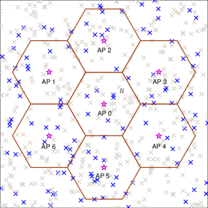
Figure 1: System model. The red stars represent APs. The black and gray crosses represent active and inactive devices, respectively.

As shown in Fig. 1, we consider a multi-cell network which consists of $M$-antenna APs and single-antenna devices. The locations of APs are distributed according to the hexagonal grid model with the side length of each hexagonal cell equal to $R$. The APs and their cells are indexed by $j$ and the set of indices of APs is denoted as $\mathcal{J}\triangleq\{0,1,\cdots\}$. The devices remain stationary or move slowly over time. The devices are indexed by $i$, and the set of indices of devices is denoted as $\mathcal{I}\triangleq\{1,2,\cdots\}$. Let $a_{i}\in\{0,1\}$ denote the activity state of device $i$, where $a_{i}=1$ indicates that device $i$ is active, and $a_{i}=0$ otherwise. Denote $\Phi_{j}$ as the set of indices of the devices in cell $j$. Let $N_{j}\triangleq|\Phi_{j}|$ denote the number of devices in cell $j$. Denote $\mathbf{a}_{j}\triangleq(a_{i})_{i\in\Phi_{j}}\in\{0,1\}^{N_{j}}$ as the activity vector of devices in cell $j$. We consider both large-scale fading and small-scale fading. Let $d_{i,j}$ denote the distance between device $i$ and AP $j$. We consider a narrow-band system [9, 14, 15, 7]. We adopt the commonly used power-law path loss model for large-scale random networks [24, 25, 26], i.e., transmitted signals with distance $d$ are attenuated with a factor $d^{-\alpha}$, where $\alpha\geq 2$ is the path loss exponent [25]. Let $\gamma_{i,j}\triangleq d_{i,j}^{-\alpha}$ denote the path loss between device $i$ and AP $j$. For small-scale fading, we consider the block fading channel model, i.e., the channel is static in each coherence block and changes across blocks in an i.i.d. manner. Let $\mathbf{h}_{i,j}\in\mathbb{C}^{M}$ denote the small-scale fading coefficient between device $i$ and AP $j$. We assume Rayleigh fading for small-scale fading, i.e., $\mathbf{h}_{i,j}$, $i\in\mathcal{I}$ and $j\in\mathcal{J}$ are i.i.d. according to $\mathcal{CN}(\mathbf{0},\mathbf{I}_{M})$.

We consider a massive access scenario arising from mMTC, where each cell contains a large number of devices, and very small of them are active in each coherence block. That is, for all $j\in\mathcal{J}$, $\sum_{i\in\Phi_{j}}a_{i}\ll N_{j}$. We adopt a grant-free massive access scheme [17, 18, 8, 19]. Specifically, each device $i$ is assigned a specific pilot sequence $\mathbf{p}_{i}=(p_{i,\ell})_{\ell\in\mathcal{L}}\in\mathbb{C}^{L}$ of length $L$, where $\mathcal{L}\triangleq\{1,2,\cdots,L\}$. Note that $L$ is much smaller than the number of devices in each cell. Let $\mathbf{P}_{j}\triangleq(\mathbf{p}_{i})_{i\in\Phi_{j}}\in\mathbb{C}^{L\times N_{j}}$ denote the $L\times N_{j}$ matrix of the pilot sequences of the devices in cell $j$. As $L\ll N_{j}$, $j\in\mathcal{J}$, it is not possible to assign mutually orthogonal pilot sequences to the devices within a cell. As in [11, 9, 14, 15, 16, 8], we assume that the pilot sequences for all devices are generated in an i.i.d. manner according to $\mathcal{CN}(\mathbf{0},\mathbf{I}_{L})$. By noting that a Gaussian random variable is continuous, the probability of assigning different devices the same pilot sequence is zero. In each coherence block, all active devices synchronously send their pilot sequences [9, 16, 8], and each AP aims to detect the activities of its associated devices (i.e., the devices in its own cell). Let $\mathbf{Y}_{j}\in\mathbb{C}^{L\times M}$ denote the received signal over the $L$ signal dimensions and $M$ antennas at AP $j$. Then, we have

$$\mathbf{Y}_{j} =\sum_{i\in\mathcal{I}}a_{i}{\color[rgb]{0,0,0}\gamma_{i,j}^{\frac{1}{2}}}\mathbf{p}_{i}\mathbf{h}_{i,j}^{T}+\mathbf{Z}_{j},\quad j\in\mathcal{J},$$

where $\mathbf{Z}_{j}\in\mathbb{C}^{L\times M}$ is the additive white Gaussian noise (AWGN) at AP $j$ with each element following $\mathcal{CN}(0,\mathbf{\delta}^{2})$. In this paper, w.l.o.g., we focus on the device activity detection at a typical AP located at the origin. The typical AP is denoted as AP $0$, and its six neighbor APs are indexed with $1,2,\cdots,6$, respectively. We consider two types of activity detection mechanisms, i.e., non-cooperative device activity detection and cooperative device activity detection. For ease of exposition, we assume that the large-scale fading powers are known for non-cooperative and cooperative activity detections.

• Non-cooperative Device Activity Detection: Let $\bm{\gamma}_{0}\triangleq(\gamma_{i,0})_{i\in\Phi_{0}}\in\mathbb{R}^{N_{0}}$ denote the path losses between the devices in cell $0$ and AP $0$. Under non-cooperative device activity detection, AP $0$ has knowledge of $\mathbf{P}_{0}$ and $\bm{\gamma}_{0}$ [9, 14, 15, 7] and would like to detect the activities of the devices in $\Phi_{0}$ from the received signal $\mathbf{Y}_{0}$.

• Cooperative Device Activity Detection: Denote $\overline{\Phi}_{0}=\cup_{j=0}^{6}\Phi_{j}$ as the set of indices of the devices in cell $0$ as well as its six neighbor cells. Denote $\overline{N}_{0}\triangleq|\overline{\Phi}_{0}|=\sum_{j=0}^{6}N_{j}$. Let $\overline{\mathbf{P}}_{0}\triangleq(\mathbf{P}_{j})_{j\in\{0,1,\cdots,6\}}\in\mathbb{C}^{L\times\overline{N}_{0}}$ denote the $L\times\overline{N}_{0}$ matrix of the pilot sequences of the devices in $\overline{\Phi}_{0}$. Let $\overline{\bm{\gamma}}_{j}\triangleq(\gamma_{i,j})_{i\in\overline{\Phi}_{0}}\in\mathbb{R}^{\overline{N}_{0}}$ denote the path losses between the devices in $\overline{\Phi}_{0}$ and AP $j$. Under cooperative device activity detection, each AP $j\in\{1,2,\cdots,6\}$ transmits its received signal $\mathbf{Y}_{j}$ or the sample covariance $\widehat{\mathbf{\Sigma}}_{\mathbf{Y}_{j}}\triangleq\frac{1}{M}\mathbf{Y}_{j}\mathbf{Y}_{j}^{H}$ (a sufficient statistics for estimating device activities, which will be seen shortly) to AP $0$ via an error-free backhaul link. AP $0$ has knowledge of $\overline{\mathbf{P}}_{0}$ and $\overline{\bm{\gamma}}_{j}$, $j\in\{0,1,\cdots,6\}$ [16] and would like to detect the activities of the devices in $\overline{\Phi}_{0}$ (i.e., the devices in its cell and its six neighbor cells) from $\overline{\mathbf{Y}}_{0}\triangleq[\mathbf{Y}_{0},\mathbf{Y}_{1},\cdots,\mathbf{Y}_{6}]\in\mathbb{C}^{L\times 7M}$ or $\widehat{\mathbf{\Sigma}}_{\mathbf{Y}_{j}}$, $j\in\{0,1,2\cdots,6\}$. Note that each AP detects activities of the devices in its six neighbor cells rather than simply treating them as interference, for the purpose of improving the accuracy for detecting the devices in $\Phi_{0}$.

Later, we shall see that with extra knowledge and observations, cooperative device activity detection can achieve high detection accuracy for the device activities in $\Phi_{0}$, at the cost of computational complexity increase, compared to non-cooperative device activity detection.

III Non-cooperative Device Activity Detection

In this section, we consider non-cooperative device activity detection, where given $\mathbf{P}_{0}$ and $\bm{\gamma}_{0}$, AP $0$ detects the activities of the devices in $\Phi_{0}$ from $\mathbf{Y}_{0}$. Then, $\mathbf{Y}_{0}$ can be rewritten as

$$\mathbf{Y}_{0} =\mathbf{P}_{0}\mathbf{A}_{0}\bm{\Gamma}_{0}^{\frac{1}{2}}\mathbf{H}_{0}^{T}+\sum_{i\in\mathcal{I}\setminus\Phi_{0}}a_{i}\gamma_{i,0}^{\frac{1}{2}}\mathbf{p}_{i}\mathbf{h}_{i,0}^{T}+\mathbf{Z}_{0},$$ (1)

where $\mathbf{A}_{0}\triangleq{\rm diag}(\mathbf{a}_{0})$, $\mathbf{\Gamma}_{0}\triangleq{\rm diag}(\bm{\gamma}_{0})$, and $\mathbf{H}_{0}\triangleq(\mathbf{h}_{i,0})_{i\in\Phi_{0}}\in\mathbb{C}^{M\times N_{0}}$. Note that the first term in (1) is the received signal from the devices in $\Phi_{0}$, and the second term is the received inter-cell interference from the other devices.

Let $\mathbf{y}_{0,m}$ denote the $m$-th column of $\mathbf{Y}_{0}$. Under Rayleigh fading and AWGN, given device activities, large-scale fading, and pilot sequences, $\mathbf{y}_{0,m}$, $m\in\{1,2,\cdots,M\}$ are i.i.d. according to $\mathcal{CN}(\mathbf{0},\mathbf{P}_{0}\mathbf{A}_{0}\bm{\Gamma}_{0}\mathbf{P}_{0}^{H}+\widetilde{\mathbf{X}}+\delta^{2}\mathbf{I}_{L})$, where $\widetilde{\mathbf{X}}\triangleq\sum\limits_{i\in\mathcal{I}\setminus\Phi_{0}}a_{i}\gamma_{i,0}\mathbf{p}_{i}\mathbf{p}_{i}^{H}\in\mathbb{C}^{L\times L}$. Here, $\mathbf{P}_{0}\mathbf{A}_{0}\bm{\Gamma}_{0}\mathbf{P}_{0}^{H}$, $\widetilde{\mathbf{X}}$, and $\delta^{2}\mathbf{I}_{L}$ are the covariance matrices of the received signal, inter-cell interference, and noise at AP $0$, respectively. Besides $\mathbf{a}_{0}$, $\widetilde{\mathbf{X}}$ is also unknown and has to be estimated. Notice that estimation of the $L\times L$ matrix $\widetilde{\mathbf{X}}$ involves very high computational complexity, especially when $L$ is moderate or large, and will yield optimization problems that are not tractable. In addition, note that $\widetilde{\mathbf{X}}$ is diagonally dominant (as shown in Fig. 2), since pilot sequences are generated from i.i.d. $\mathcal{CN}(\mathbf{0},\mathbf{I}_{L})$ [19]. Therefore, we approximate $\widetilde{\mathbf{X}}$ with $\mathbf{X}\triangleq{\rm diag}(\mathbf{x})$, where $\mathbf{x}\triangleq(x_{\ell})_{\ell\in\mathcal{L}}\in[0,\infty)^{L}$[16, 27, 28]. Fig. 2 demonstrates that the approximation is reasonable and has a negligible error when there are massive interfering devices. Later, we shall see that allowing the entries of $\mathbf{x}$ to be different facilitates the coordinate descent optimization in device activity detection. Note that $\mathbf{x}$ can be interpreted as the interference powers at the $L$ signal dimensions. In addition, rewriting $\mathbf{X}$ as $\sum_{\ell\in\mathcal{L}}x_{\ell}\mathbf{e}_{\ell}\mathbf{e}_{\ell}^{H}$, where $\mathbf{e}_{\ell}$ is the $\ell$-th standard basis which has a $1$ as its $\ell$-th entry and $0$s elsewhere, the inter-cell interference can be viewed as from $L$ active devices with pilots $\mathbf{e}_{\ell}$, $\ell\in\mathcal{L}$ and path losses $x_{\ell}$, $\ell\in\mathcal{L}$. Under the approximation of $\widetilde{\mathbf{X}}$, the distribution of $\mathbf{y}_{0,m}$ is approximated by

$$\mathbf{y}_{0,m}\sim\mathcal{CN}\left(\mathbf{0},\mathbf{P}_{0}\mathbf{A}_{0}\bm{\Gamma}_{0}\mathbf{P}_{0}^{H}+\mathbf{X}+\delta^{2}\mathbf{I}_{L}\right),\quad m\in\{1,2,\cdots,M\}.$$ (2)

Based on (2) and the fact that $\mathbf{y}_{0,m}$, $m\in\{1,2,\cdots,M\}$ are i.i.d., the likelihood of $\mathbf{Y}_{0}$ is given by

$$f_{\mathbf{a}_{0},\mathbf{x}}(\mathbf{Y}_{0})\propto\frac{\exp\left(-{\rm tr}\left(\left(\mathbf{P}_{0}\mathbf{A}_{0}\bm{\Gamma}_{0}\mathbf{P}_{0}^{H}+\mathbf{X}+\delta^{2}\mathbf{I}_{L}\right)^{-1}\mathbf{Y}_{0}\mathbf{Y}_{0}^{H}\right)\right)}{|(\mathbf{P}_{0}\mathbf{A}_{0}\bm{\Gamma}_{0}\mathbf{P}_{0}^{H}+\mathbf{X}+\delta^{2}\mathbf{I}_{L})|^{M}},$$ (3)

where $\propto$ means “proportional to”, $|\cdot|$ is the determinant of a matrix, and ${\rm tr}(\cdot)$ is the trace of a matrix. Note that the constant coefficient is omitted for notation simplicity. From (3), we know that $f_{\mathbf{a}_{0},\mathbf{x}}(\mathbf{Y}_{0})$ depends on $\mathbf{Y}_{0}$ only through the sample covariance matrix $\widehat{\mathbf{\Sigma}}_{\mathbf{Y}_{0}}$. Thus, $\widehat{\mathbf{\Sigma}}_{\mathbf{Y}_{0}}$ is a sufficient statistics for estimating $\mathbf{a}_{0}$ and $\mathbf{x}$. Based on (3), in the following, we consider the joint ML estimation and joint MAP estimation of $N_{0}$ device activities $\mathbf{a}_{0}$ and $L$ interference powers $\mathbf{x}$, respectively.

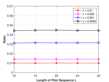
Figure 2: Average ratio $\mathbb{E}\left[\frac{\tilde{X}_{i,j}}{\tilde{X}_{i,i}}\right]$, $i,j\in\mathcal{L}$ and $j\neq i$, where $\tilde{X}_{i,j}$ denotes the element in the $i$-th row and the $j$-th column of $\widetilde{\mathbf{X}}$. Active interfering devices in $\mathcal{I}\setminus\Phi_{0}$ are assumed to follow a homogeneous Poisson point process (PPP) with density $\lambda$. $R=200$ and $\alpha=3$. Note that the non-diagonal elements of $\widetilde{\mathbf{X}}$ are i.i.d., and the diagonal elements of $\widetilde{\mathbf{X}}$ are i.i.d. The expectation is evaluated via Monte Carlo simulations.

III-A Joint ML Estimation of Device Activities and Interference Powers

In this part, we perform the joint ML estimation of $\mathbf{a}_{0}$ and $\mathbf{x}$. The maximization of the likelihood $f_{\mathbf{a}_{0},\mathbf{x}}(\mathbf{Y}_{0})$ is equivalent to the minimization of the negative log-likelihood $-\log{\color[rgb]{0,0,0}f_{\mathbf{a}_{0},\mathbf{x}}(\mathbf{Y}_{0})}\\ \propto f_{\rm ML}(\mathbf{a}_{0},\mathbf{x})$, where

$$f_{\rm ML}(\mathbf{a}_{0},\mathbf{x})\triangleq\log|\mathbf{P}_{0}\mathbf{A}_{0}\mathbf{\Gamma}_{0}\mathbf{P}_{0}^{H}+\mathbf{X}+\delta^{2}\mathbf{I}_{L}|+{\rm tr}((\mathbf{P}_{0}\mathbf{A}_{0}\mathbf{\Gamma}_{0}\mathbf{P}_{0}^{H}+\mathbf{X}+\delta^{2}\mathbf{I}_{L})^{-1}\widehat{\mathbf{\Sigma}}_{\mathbf{Y}_{0}}),$$ (4)

with $\widehat{\mathbf{\Sigma}}_{\mathbf{Y}_{0}}=\frac{1}{M}\mathbf{Y}_{0}\mathbf{Y}_{0}^{H}$. By omitting the constant term in the negative log-likelihood function, the joint ML estimation of $\mathbf{a}_{0}$ and $\mathbf{x}$ without AP cooperation is formulated as follows.

Problem 1 (Joint ML Estimation without AP Cooperation)

$$\min_{\mathbf{a}_{0},\mathbf{x}} \quad f_{\rm ML}(\mathbf{a}_{0},\mathbf{x})$$

$$s.t. \quad 1\geq a_{i}\geq 0,\quad i\in\Phi_{0},$$ (5)

$$\quad x_{\ell}\geq 0,\quad\ell\in\mathcal{L}.$$ (6)

Let $(\mathbf{a}_{0}^{*},\mathbf{x}^{*})$ denote an optimal solution of Problem 1.

Note that in this paper, binary condition $a_{i}\in\{0,1\}$ is relaxed to continuous condition $a_{i}\in[0,1]$ in each estimation problem, and binary detection results are obtained by performing thresholding after solving the estimation problem as in [17] and [8]. Different from the ML estimation in [17] and [8], which only focuses on estimating $\mathbf{a}_{0}$ in a single-cell network without inter-cell interference, Problem 1 considers the joint ML estimation of $\mathbf{a}_{0}$ and $\mathbf{x}$ in the multi-cell network with inter-cell interference. As $\log|\mathbf{P}_{0}\mathbf{A}_{0}\mathbf{\Gamma}_{0}\mathbf{P}_{0}^{H}+\mathbf{X}+\delta^{2}\mathbf{I}_{L}|$ is a concave function of $\mathbf{a}_{0}$ and $\mathbf{x}$, and ${\rm tr}((\mathbf{P}_{0}\mathbf{A}_{0}\mathbf{\Gamma}_{0}\mathbf{P}_{0}^{H}+\mathbf{X}+\delta^{2}\mathbf{I}_{L})^{-1}\widehat{\mathbf{\Sigma}}_{\mathbf{Y}_{0}})$ is a convex function of $\mathbf{a}_{0}$ and $\mathbf{x}$, $f_{\rm ML}(\mathbf{a}_{0},\mathbf{x})$ is a difference of convex (DC) function. Combining with the fact that the inequality constraints are linear, Problem 1 is a DC programming problem, which is a subcategory of non-convex problems. Note that obtaining a stationary point is the classic goal for solving a non-convex problem. In the following, we extend the coordinate descent method for the case without inter-cell interference in [17] to obtain a stationary point of Problem 1 for the case with inter-cell interference. As a closed-form optimal solution can be obtained for the optimization of each coordinate, the coordinate descent method is more computationally efficient than standard methods for DC programming, such as convex-concave procedure, where the convex approximate problem in each iteration cannot be solved analytically.

In each iteration of the proposed coordinate descent algorithm, all coordinates are updated once. At each step of one iteration, we optimize $f_{\rm ML}(\mathbf{a}_{0},\mathbf{x})$ with respect to one of the coordinates in $\{a_{i}$: $i\in\Phi_{0}\}\cup\{x_{\ell}:\ell\in\mathcal{L}\}$. Specifically, given $\mathbf{a}_{0}$ and $\mathbf{x}$ obtained in the previous step, the coordinate descent optimization with respect to $a_{i}$ is equivalent to the optimization of the increment $d$ in $a_{i}$:

$$\min_{1-a_{i}\geq d\geq-a_{i}}\ f_{\rm ML}(\mathbf{a}_{0}+d\mathbf{e}_{i},\mathbf{x}),$$ (7)

and the coordinate descent optimization with respect to $x_{\ell}$ is equivalent to the optimization of the increment $d$ in $x_{\ell}$:

$$\min_{d\geq-x_{\ell}}\ f_{\rm ML}(\mathbf{a}_{0},\mathbf{x}+d\mathbf{e}_{\ell}).$$ (8)

Based on structural properties of the coordinate descent optimization problems in (7) and (8), we can derive their closed-form optimal solutions.

Theorem 1 (Optimal Solutions of Coordinate Descent Optimizations in (7) and (8))

Given $\mathbf{a}_{0}$ and $\mathbf{x}$ obtained in the previous step, the optimal solution of the coordinate optimization with respect to the increment in $a_{i}$ in (7) is given by

$$\min\left\{\max\left\{\frac{\mathbf{p}_{i}^{H}\mathbf{\Sigma}^{-1}\widehat{\mathbf{\Sigma}}_{\mathbf{Y}_{0}}\mathbf{\Sigma}^{-1}\mathbf{p}_{i}-\mathbf{p}_{i}^{H}\mathbf{\Sigma}^{-1}\mathbf{p}_{i}}{\gamma_{i,0}(\mathbf{p}_{i}^{H}\mathbf{\Sigma}^{-1}\mathbf{p}_{i})^{2}},-a_{i}\right\},1-a_{i}\right\},$$ (9)

and the optimal solution of the coordinate optimization with respect to the increment in $x_{\ell}$ in (8) is given by

$$\max\left\{\frac{\mathbf{e}_{\ell}^{H}\mathbf{\Sigma}^{-1}\widehat{\mathbf{\Sigma}}_{\mathbf{Y}_{0}}\mathbf{\Sigma}^{-1}\mathbf{e}_{\ell}-\mathbf{e}_{\ell}^{H}\mathbf{\Sigma}^{-1}\mathbf{e}_{\ell}}{(\mathbf{e}_{\ell}^{H}\mathbf{\Sigma}^{-1}\mathbf{e}_{\ell})^{2}},-x_{\ell}\right\}.$$ (10)

Here, $\mathbf{\Sigma}\triangleq\mathbf{P}_{0}\mathbf{A}_{0}\bm{\Gamma}_{0}\mathbf{P}_{0}^{H}+\mathbf{X}+\delta^{2}\mathbf{I}_{L}$ is determined by $\mathbf{a}_{0}$ and $\mathbf{x}$.

Proof:

Please refer to Appendix A. ∎

TABLE I: Computational complexity of each iteration of an iterative algorithm.

Estimation algorithm	Computational complexity of each iteration
joint ML estimation in non-cooperative mechanism	$\mathcal{O}(N_{0}L^{2}+L^{3})$
joint MAP estimation in non-cooperative mechanism	$\mathcal{O}(N_{0}2^{N_{0}}+N_{0}L^{2}+L^{3})$
joint ML estimation in cooperative mechanism	$\mathcal{O}(\overline{N}_{0}L^{2}+L^{3})$
joint MAP estimation in cooperative mechanism	$\mathcal{O}(\sum_{j=0}^{6}N_{j}2^{N_{j}}+\overline{N}_{0}L^{2}+L^{3})$
ML estimation in [17]	$\mathcal{O}(NL^{2})$

The details of the coordinate descent algorithm for solving Problem 1 are summarized in Algorithm 1. Specifically, in Steps $4-6$, each coordinate of $\mathbf{a}_{0}$ is updated. In Steps $9-11$, each coordinate of $\mathbf{x}$ is updated. Unlike the coordinate descent algorithm for the ML estimation in [17] which only updates the coordinates of $\mathbf{a}_{0}$, the coordinate updates in Algorithm 1 for the joint ML estimation are with respect to both $\mathbf{a}_{0}$ and $\mathbf{x}$. In addition, as in [8], we update $\mathbf{\Sigma}^{-1}$ instead of $\mathbf{\Sigma}$ in each coordinate descent optimization (i.e., Steps $6$ and $11$), which avoids the calculation of matrix inversion and improves the computation efficiency (the proof for the update of $\mathbf{\Sigma}^{-1}$ can be found in Appendix A). As shown in Table I, the computational complexity of each iteration of Algorithm 1 for the joint ML estimation is higher than the one for the ML estimation in [17] due to the extra estimation of $\mathbf{x}_{0}$. As $f_{\rm ML}(\mathbf{a}_{0},\mathbf{x})$ is continuously differentiable, and each of the coordinate optimizations in (7) and (8) has a unique optimal solution, by[29, Proposition 2.7.1], we know that Algorithm 1 for the joint ML estimation converges to a stationary point of Problem 1, as the number of iterations goes to infinity.

Algorithm 1 Coordinate Descent Algorithm without AP Cooperation

1:  Initialize $\mathbf{\Sigma}^{-1}=\frac{1}{\delta^{2}}\mathbf{I}_{L}$, $\mathbf{a}_{0}=\mathbf{0}$, $\mathbf{x}=\mathbf{0}$.

2:  repeat

3:  for $i\in\Phi_{0}$ do

4:     ML: Calculate $d$ according to (9).

5:     MAP: Calculate $d$ according to (16).

6:     Update $a_{i}=a_{i}+d$ and $\mathbf{\Sigma}^{-1}=\mathbf{\Sigma}^{-1}-\frac{d\gamma_{i,0}\mathbf{\Sigma}^{-1}\mathbf{p}_{i}\mathbf{p}_{i}^{H}\mathbf{\Sigma}^{-1}}{1+d\gamma_{i,0}\mathbf{p}_{i}^{H}\mathbf{\Sigma}^{-1}\mathbf{p}_{i}}$.

7:  end for

8:  for $\ell\in\mathcal{L}$ do

9:     ML: Calculate $d$ according to (10).

10:     MAP: Calculate $d$ according to (17).

11:     Update $x_{\ell}=x_{\ell}+d$ and $\mathbf{\Sigma}^{-1}=\mathbf{\Sigma}^{-1}-\frac{d\mathbf{\Sigma}^{-1}\mathbf{e}_{\ell}\mathbf{e}_{\ell}^{H}\mathbf{\Sigma}^{-1}}{1+d\mathbf{e}_{\ell}^{H}\mathbf{\Sigma}^{-1}\mathbf{e}_{\ell}}$.

12:  end for

13:  until $(\mathbf{a}_{0},\mathbf{x})$ satisfies some stopping criterion.

III-B Joint MAP Estimation of Device Activities and Interference Powers

In this part, we assume that $\mathbf{a}_{0}$ and $\mathbf{x}$ are random and perform the joint MAP estimation of $\mathbf{a}_{0}$ and $\mathbf{x}$.

III-B1 Prior Distributions

We assume that $\mathbf{a}_{0}$ and $\mathbf{x}$ are independently distributed. Note that this is a weak assumption, as it only requires that the device activities in cell $0$ are independent of those in the other cells. First, we introduce a general prior distribution of the Bernoulli random vector $\mathbf{a}_{0}$. Unlike [16] where devices in a cell are assumed to access the channel in an i.i.d. manner, we allow for correlation among the activities of the devices in cell $0$. In particular, we adopt the multivariate Bernoulli (MVB) model for $\mathbf{a}_{0}$ [23]. The probability mass function (p.m.f.) of $\mathbf{a}_{0}$ under the MVB model is given by

$$p_{0}\left(\mathbf{a}_{0}\right)=\exp\left(\sum_{\omega\in\Psi_{0}}\left(c_{\omega}\prod_{i\in\omega}a_{i}\right)+b_{0}\right),$$ (11)

where $\Psi_{0}$ denotes the set of nonempty subsets of $\Phi_{0}$, $c_{\omega}$ is the coefficient reflecting the correlation among $a_{i}$, $i\in\omega$, and $b_{0}\triangleq-\log(\sum_{\mathbf{a}_{0}\in\{0,1\}^{N_{0}}}\exp(\sum_{\omega\in\Psi_{0}}(c_{\omega}\prod_{i\in\omega}a_{i})))$ is the normalization factor. Note that $c_{\omega}$, $\omega\in\Psi_{0}$ can be estimated based on the historical device activity data using existing methods [23]. In addition, given the p.m.f. of $\mathbf{a}_{0}$ in any form, the coefficients $c_{\omega}$, $\omega\in\Psi_{0}$ can be calculated according to [23, Lemma $2.1$]. When $c_{\omega}=0$ for all $|\omega|>2$, the MVB model reduces to the Ising model [30]. When $c_{\omega}=0$ for all $|\omega|>1$, the MVB model reduces to the independent model with $\Pr(a_{i}=1)=\frac{\exp\left(c_{\{i\}}\right)}{\exp\left(c_{\{i\}}\right)+1}$, $i\in\Phi_{0}$. When $c_{\omega}=0$ for all $|\omega|>1$ and $c_{\omega}=c$ for all $|\omega|=1$, the MVB model reduces to the i.i.d. model in [16] with $\Pr(a_{i}=1)=\frac{\exp\left(c\right)}{\exp\left(c\right)+1}$, $i\in\Phi_{0}$.

To further illustrate the MVB model, we present two instances of $p_{0}(\mathbf{a}_{0})$ under group device activity. In both instances, the devices in $\Phi_{0}$ are divided into $K$ groups and the device activities in different groups are independent. For all $k\in\mathcal{K}\triangleq\{1,2,\cdots,K\}$, let $\mathcal{G}_{k}\subseteq\Phi_{0}$ denote the set of indices of the devices in the $k$-th group. Note that $\cup_{k\in\mathcal{K}}\mathcal{G}_{k}=\Phi_{0}$ and $\mathcal{G}_{k}\cap\mathcal{G}_{k^{\prime}}=\emptyset$ for $k,k^{\prime}\in\mathcal{K}$, $k\neq k^{{}^{\prime}}$. According to[23, Theorem 2.1], we have

$$c_{\omega}=0,\quad\nexists\ k\in\mathcal{K}\text{ such that }\omega\subseteq\mathcal{G}_{k}.$$ (12)

It remains to specify $c_{\omega}$, $\omega\subseteq\mathcal{G}_{k}$, $k\in\mathcal{K}$ in the two instances.

• First Instance: Each group contains two devices, i.e., $|\mathcal{G}_{k}|=2$, $k\in\mathcal{K}$; every two devices in a group are correlated with correlation coefficient $\eta$; $\Pr[a_{i}=1]=p_{a}$, $i\in\Phi_{0}$. Consequently, for two devices $i_{1}$ and $i_{2}$ in one group, $\Pr(a_{i_{1}}=1,a_{i_{2}}=1)=\eta p_{a}+(1-\eta)p_{a}^{2}$, $\Pr(a_{i_{1}}=0,a_{i_{2}}=1)=\Pr(a_{i_{1}}=1,a_{i_{2}}=0)=(1-\eta)(p_{a}-p_{a}^{2})$ and $\Pr(a_{i_{1}}=0,a_{i_{2}}=0)=1+(\eta-2)p_{a}+(1-\eta)p_{a}^{2}$. According to  [23, Lemma $2.1$], we know that $p_{0}(\mathbf{a}_{0})$ satisfies (11) with $c_{\omega}$ satisfying (12) and

  $$c_{\omega}= \begin{cases}\frac{(\eta p_{a}+(1-\eta)p_{a}^{2})(1+(\eta-2)p_{a}+(1-\eta)p_{a}^{2})}{(1-\eta)^{2}(p_{a}-p_{a}^{2})^{2}}\quad&|\omega|=2\\ \frac{(1-\eta)(p_{a}-p_{a}^{2})}{1+(\eta-2)p_{a}+(1-\eta)p_{a}^{2}}&|\omega|=1\end{cases},\quad\omega\subseteq\mathcal{G}_{k},k\in\mathcal{K}.$$

• Second Instance: The activity states of devices in a group are the same, i.e., $a_{i}$, $i\in\mathcal{G}_{k}$ are the same for all $k\in\mathcal{K}$, implying $\sum_{i\in\mathcal{G}_{k}}a_{i}\in\{0,|\mathcal{G}_{k}|\}$, $k\in\mathcal{K}$; $\Pr[\cap_{i\in\mathcal{G}_{k}}(a_{i}=1)]=p_{k}$, $k\in\mathcal{K}$. According to [23, Lemma $2.1$], we know that $p_{0}(\mathbf{a}_{0})$ approaches (11) with $c_{\omega}$ satisfying (12) and

  $$c_{\omega}= \begin{cases}(-1)^{|\omega|}\log(\frac{1-p_{k}}{\epsilon})\quad&|\omega|<|\mathcal{G}_{k}|\\ \log(\frac{p_{k}}{1-p_{k}})&|\omega|=|\mathcal{G}_{k}|,|\omega|\text{ is odd}\\ \log(\frac{p_{k}(1-p_{k})}{\epsilon^{2}})&|\omega|=|\mathcal{G}_{k}|,|\omega|\text{ is even}\\ \end{cases},\quad\omega\subseteq\mathcal{G}_{k},k\in\mathcal{K},$$

  where $\epsilon>0$, as $\epsilon\to 0$. Note that in this instance, $p_{0}(\mathbf{a}_{0})$ can be well approximated by (11) with a small $\epsilon$.

Next, we derive a prior distribution of $\mathbf{x}$. Under non-cooperative device activity detection, the locations of the active interfering devices in $\mathcal{I}\setminus\Phi_{0}$ are assumed to follow a homogeneous Poisson point process (PPP) with density $\lambda$, which is a widely adopted model for large-scale wireless networks [25]. As pilot sequences are generated from i.i.d. $\mathcal{CN}(\mathbf{0},\mathbf{I}_{L})$, we assume that $x_{\ell}$, $\ell\in\mathcal{L}$ are i.i.d. with the same distribution as $\sum_{i\in\mathcal{I}\setminus\Phi_{0}}a_{i}\gamma_{i,0}$. Therefore, $x_{\ell}$ is a power-law shot noise, whose exact distribution is still unknown [25]. As in [31], we approximate the probability density function (p.d.f.) of $x_{\ell}$ with a Gaussian distribution using moment matching. Note that the Gaussian approximation is accurate when the cell size (i.e., $R$) is large [31, 32]. Based on the above assumptions and techniques from stochastic geometry, we have the following results.

Lemma 1 (Approximated Distribution of $\mathbf{x}$)

The p.d.f. of $\mathbf{x}$ is approximated by

$$g(\mathbf{x})=\frac{1}{(\sqrt{2\pi}\sigma)^{L}}\exp\left(-\frac{\sum_{\ell\in\mathcal{L}}(x_{\ell}-\mu)^{2}}{2\sigma^{2}}\right),$$

where $\mu=12\lambda\int_{\frac{\sqrt{3}}{2}R}^{\infty}\int_{0}^{\frac{\sqrt{3}}{3}x}(x^{2}+y^{2})^{-\frac{\alpha}{2}}{\rm d}y{\rm d}x$ and $\sigma^{2}=12\lambda\int_{\frac{\sqrt{3}}{2}R}^{\infty}\int_{0}^{\frac{\sqrt{3}}{3}x}(x^{2}+y^{2})^{-\alpha}{\rm d}y{\rm d}x$.

Proof:

Please refer to Appendix B. ∎

The integral expressions of $\mu$ and $\sigma^{2}$ in Lemma 1 are for the case where cell $0$ is modeled as a hexagon with side length $R$. If cell $0$ is modeled as a disk with radius $R$, $\mu$ and $\sigma^{2}$ have closed-form expressions, i.e., $\mu=\frac{2\pi\lambda R^{2-\alpha}}{\alpha-2}$ and $\sigma^{2}=\frac{\pi\lambda R^{2-2\alpha}}{\alpha-1}$, and the following results for non-cooperative device activity detection still hold. Fig. 3 plots the histogram of $x_{\ell}$ (which reflects the shape of the p.d.f. of $x_{\ell}$) and the Gaussian distribution with the same mean and variance. From Fig. 3, we can see that the Gaussian distribution is a good approximation of the exact p.d.f. of $x_{\ell}$, which verifies Lemma 1.

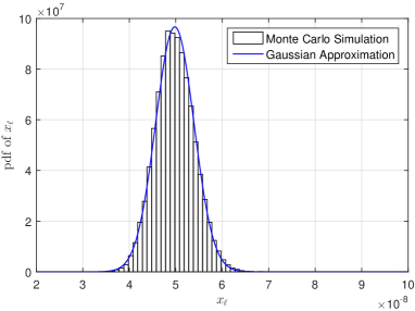
Figure 3: Comparison between the p.d.f. of $x_{\ell}$ and its corresponding Gaussian approximation. $R=200$, $\lambda=0.0005$ and $\alpha=4$.

III-B2 Joint MAP Estimation

Based on the conditional density of $\mathbf{Y}_{0}$ given $\mathbf{a}_{0}$ and $\mathbf{x}$ (identical to the likelihood of $\mathbf{Y}_{0}$ in the joint ML estimation) and the prior distributions of $\mathbf{a}_{0}$ and $\mathbf{x}$, the conditional joint density of $\mathbf{a}_{0}$ and $\mathbf{x}$, given $\mathbf{Y}_{0}$, is given by

$${\color[rgb]{0,0,0}f_{\mathbf{a}_{0},\mathbf{x}|\mathbf{Y}_{0}}(\mathbf{a}_{0},\mathbf{x},\mathbf{Y}_{0})\propto f_{\mathbf{a}_{0},\mathbf{x}}(\mathbf{Y}_{0})}p_{0}(\mathbf{a}_{0})g(\mathbf{x})$$

$$\propto\frac{\exp\left(-{\rm tr}\left(\left(\mathbf{P}_{0}\mathbf{A}_{0}\mathbf{\Gamma}_{0}\mathbf{P}_{0}^{H}+\mathbf{X}+\delta^{2}\mathbf{I}_{L}\right)^{-1}\mathbf{Y}_{0}\mathbf{Y}_{0}^{H}\right)-\sum_{\ell\in\mathcal{L}}\frac{(x_{\ell}-\mu)^{2}}{2\sigma^{2}}+\sum_{\omega\in\Psi_{0}}\left(c_{\omega}\prod_{i\in\omega}a_{i}\right)\right)}{|(\mathbf{P}_{0}\mathbf{A}_{0}\bm{\Gamma}_{0}\mathbf{P}_{0}^{H}+\mathbf{X}+\delta^{2}\mathbf{I}_{L})|^{M}}.$$

The maximization of the conditional joint density $f_{\mathbf{a}_{0},\mathbf{x}|\mathbf{Y}_{0}}(\mathbf{a}_{0},\mathbf{x},\mathbf{Y}_{0})$ is equivalent to the minimization of the negative logarithm of the conditional joint density $-\log{\color[rgb]{0,0,0}f_{\mathbf{a}_{0},\mathbf{x}|\mathbf{Y}_{0}}(\mathbf{a}_{0},\mathbf{x},\mathbf{Y}_{0})}\propto f_{\rm MAP}(\mathbf{a}_{0},\mathbf{x})$, where

$$f_{\rm MAP}(\mathbf{a}_{0},\mathbf{x})\triangleq f_{\rm ML}(\mathbf{a}_{0},\mathbf{x})+\frac{1}{2M\sigma^{2}}\sum_{\ell\in\mathcal{L}}(x_{\ell}-\mu)^{2}-\frac{1}{M}\sum_{\omega\in\Psi_{0}}\left(c_{\omega}\prod_{i\in\omega}a_{i}\right).$$ (13)

Note that $\frac{1}{2M\sigma^{2}}\sum_{\ell\in\mathcal{L}}(x_{\ell}-\mu)^{2}$ is from the p.d.f. of $\mathbf{x}$ and $-\frac{1}{M}\sum_{\omega\in\Psi_{0}}(c_{\omega}\prod_{i\in\omega}a_{i})$ is from the p.m.f. of $\mathbf{a}_{0}$. The joint MAP estimation of $\mathbf{a}_{0}$ and $\mathbf{x}$ without AP cooperation can be formulated as follows.

Problem 2 (Joint MAP Estimation without AP Cooperation)

$$\min_{\mathbf{a}_{0},\mathbf{x}} \quad f_{\rm MAP}(\mathbf{a}_{0},\mathbf{x})$$

$$s.t. \quad\eqref{eqn:single_a},\eqref{eqn:single_x}.$$

Let $(\mathbf{a}_{0}^{\dagger},\mathbf{x}^{\dagger})$ denote an optimal solution of Problem 2.

By comparing $f_{\rm MAP}(\mathbf{a}_{0},\mathbf{x})$ with $f_{\rm ML}(\mathbf{a}_{0},\mathbf{x})$, we can draw the following conclusions. The incorporation of prior distribution $g(\mathbf{x})$ pushes the estimate of $x_{\ell}$ towards its mean $\mu$ for all $\ell\in\mathcal{L}$. The incorporation of the prior distribution $p_{0}(\mathbf{a}_{0})$ pushes the estimate of $\mathbf{a}_{0}$ to the activity states with high probabilities. As $f_{\rm MAP}(\mathbf{a}_{0},\mathbf{x})-f_{\rm ML}(\mathbf{a}_{0},\mathbf{x})$ decreases with $M$, the impacts of the prior distributions of $\mathbf{a}_{0}$ and $\mathbf{x}$ reduce as $M$ increases. As $M\to\infty$, $f_{\rm MAP}(\mathbf{a}_{0},\mathbf{x})\to f_{\rm ML}(\mathbf{a}_{0},\mathbf{x})$, Problem 2 reduces to Problem 1, and $(\mathbf{a}_{0}^{\dagger},\mathbf{x}^{\dagger})$ becomes $(\mathbf{a}_{0}^{*},\mathbf{x}^{*})$.

As $f_{\rm ML}(\mathbf{a}_{0},\mathbf{x})$ is a DC function and $-\frac{1}{M}\sum_{\omega\in\Psi_{0}}(c_{\omega}\prod_{i\in\omega}a_{i})$ is a non-convex function, we can see that Problem 2 is a challenging non-convex problem with a complicated objective function. We adopt the coordinate descent method to obtain a stationary point to Problem 2. Specifically, given $\mathbf{a}_{0}$ and $\mathbf{x}$ obtained in the previous step, the coordinate descent optimization with respect to $a_{i}$, $i\in\Phi_{0}$ is equivalent to the optimization of the increment $d$ in $a_{i}$:

$$\min_{1-a_{i}\geq d\geq-a_{i}}\ f_{\rm MAP}(\mathbf{a}_{0}+d\mathbf{e}_{i},\mathbf{x}),$$ (14)

and the coordinate descent optimization with respect to $x_{\ell}$, $\ell\in\mathcal{L}$ is equivalent to the optimization of the increment $d$ in $x_{\ell}$:

$$\min_{d\geq-x_{\ell}}\ f_{\rm MAP}(\mathbf{a}_{0},\mathbf{x}+d\mathbf{e}_{\ell}).$$ (15)

Define

$$f_{a,i}(d,\mathbf{a}_{0},\mathbf{x})\triangleq\log(1+d\gamma_{i,0}\mathbf{p}_{i}^{H}\mathbf{\Sigma}^{-1}\mathbf{p}_{i})-\frac{d\gamma_{i,0}\mathbf{p}_{i}^{H}\mathbf{\Sigma}^{-1}\widehat{\mathbf{\Sigma}}_{\mathbf{Y}_{0}}\mathbf{\Sigma}^{-1}\mathbf{p}_{i}}{1+d\gamma_{i,0}\mathbf{p}_{i}^{H}\mathbf{\Sigma}^{-1}\mathbf{p}_{i}}-\frac{d}{M}\sum_{\omega\in\Psi_{0}:i\in\omega}\left(c_{\omega}\prod_{i^{{}^{\prime}}\in\omega,i^{{}^{\prime}}\neq i}a_{i^{{}^{\prime}}}\right),$$

$$f_{x,\ell}(d,\mathbf{a}_{0},\mathbf{x})\triangleq\log(1+d\mathbf{e}_{\ell}^{H}\mathbf{\Sigma}^{-1}\mathbf{e}_{\ell})-\frac{d\mathbf{e}_{\ell}^{H}\mathbf{\Sigma}^{-1}\widehat{\mathbf{\Sigma}}_{\mathbf{Y}_{0}}\mathbf{\Sigma}^{-1}\mathbf{e}_{\ell}}{1+d\mathbf{e}_{\ell}^{H}\mathbf{\Sigma}^{-1}\mathbf{e}_{\ell}}+\frac{(x_{\ell}-\mu+d)^{2}}{2M\sigma^{2}},$$

$$h_{x,\ell}(d,\mathbf{a}_{0},\mathbf{x})\triangleq\frac{\mathbf{e}_{\ell}^{H}\mathbf{\Sigma}^{-1}\mathbf{e}_{\ell}}{1+d\mathbf{e}_{\ell}^{H}\mathbf{\Sigma}^{-1}\mathbf{e}_{\ell}}-\frac{\mathbf{e}_{\ell}^{H}\mathbf{\Sigma}^{-1}\widehat{\mathbf{\Sigma}}_{\mathbf{Y}_{0}}\mathbf{\Sigma}^{-1}\mathbf{e}_{\ell}}{(1+d\mathbf{e}_{\ell}^{H}\mathbf{\Sigma}^{-1}\mathbf{e}_{\ell})^{2}}+\frac{d+x_{\ell}-\mu}{M\sigma^{2}}.$$

We write $f_{a,i}(d,\mathbf{a}_{0},\mathbf{x})$, $f_{x,\ell}(d,\mathbf{a}_{0},\mathbf{x})$, and $h_{x,\ell}(d,\mathbf{a}_{0},\mathbf{x})$ as functions of $\mathbf{a}_{0}$ and $\mathbf{x}$, as $\mathbf{\Sigma}$ is a function of $\mathbf{a}_{0}$ and $\mathbf{x}$. Note that $h_{x,\ell}(d,\mathbf{a}_{0},\mathbf{x})$ is the derivative function of $f_{x,\ell}(d,\mathbf{a}_{0},\mathbf{x})$ with respect to $d$. Denote $\mathcal{X}_{\ell}(\mathbf{a}_{0},\mathbf{x})\triangleq\{d\geq-x_{\ell}:h_{x,\ell}(d,\mathbf{a}_{0},\mathbf{x})=0\}$ as the set of roots of equation $h_{x,\ell}(d,\mathbf{a}_{0},\mathbf{x})=0$ that are no smaller than $-x_{\ell}$, for given $\mathbf{a}_{0}$ and $\mathbf{x}$. Based on structural properties of the coordinate descent optimization problems in (14) and (15), we have the following results.

Theorem 2 (Optimal Solutions of Coordinate Descent Optimizations in (14) and (15))

Given $\mathbf{a}_{0}$ and $\mathbf{x}$ obtained in the previous step, the optimal solution of the coordinate optimization with respect to the increment in $a_{i}$ in (14) is given by

$$\begin{cases}\min\left\{\max\left\{s_{i}(\mathbf{a}_{0},\mathbf{x}),-a_{i}\right\},1-a_{i}\right\},&C_{i}\leq 0\\ \arg\min_{d\in\{s_{i}(\mathbf{a}_{0},\mathbf{x}),-a_{i}+1\}}f_{a,i}(d,\mathbf{a}_{0},\mathbf{x}),&{\color[rgb]{0,0,0}0<C_{i}<\frac{\gamma_{i,0}(\mathbf{p}_{i}^{H}\mathbf{\Sigma}^{-1}\mathbf{p}_{i})^{2}}{4\mathbf{p}_{i}^{H}\mathbf{\Sigma}^{-1}\widehat{\mathbf{\Sigma}}_{\mathbf{Y}_{0}}\mathbf{\Sigma}^{-1}\mathbf{p}_{i}}}\\ -a_{i}+1,&{\color[rgb]{0,0,0}C_{i}\geq\frac{\gamma_{i,0}(\mathbf{p}_{i}^{H}\mathbf{\Sigma}^{-1}\mathbf{p}_{i})^{2}}{4\mathbf{p}_{i}^{H}\mathbf{\Sigma}^{-1}\widehat{\mathbf{\Sigma}}_{\mathbf{Y}_{0}}\mathbf{\Sigma}^{-1}\mathbf{p}_{i}}}\end{cases},$$ (16)

where $s_{i}(\mathbf{a}_{0},\mathbf{x})\triangleq\frac{1}{2C_{i}}\left(1-\sqrt{1-\frac{4C_{i}\mathbf{p}_{i}^{H}\mathbf{\Sigma}^{-1}\widehat{\mathbf{\Sigma}}_{\mathbf{Y}_{0}}\mathbf{\Sigma}^{-1}\mathbf{p}_{i}}{\gamma_{i,0}(\mathbf{p}_{i}^{H}\mathbf{\Sigma}^{-1}\mathbf{p}_{i})^{2}}}\right)-\frac{1}{\gamma_{i,0}\mathbf{p}_{i}^{H}\mathbf{\Sigma}^{-1}\mathbf{p}_{i}}$ and $C_{i}\triangleq\frac{1}{M}\sum_{\omega\in\Psi_{0}:i\in\omega}\big{(}c_{\omega}\\ \times\prod_{i^{{}^{\prime}}\in\omega,i^{{}^{\prime}}\neq i}a_{i^{{}^{\prime}}}\big{)}$, and the optimal solution of the coordinate optimization with respect to the increment in $x_{\ell}$ in (15) is given by

$$\mathop{\arg\min}\limits_{d\in\mathcal{X}_{\ell}(\mathbf{a}_{0},\mathbf{x})\cup\{-x_{\ell}\}}f_{x,\ell}(d,\mathbf{a}_{0},\mathbf{x}).$$ (17)

Proof:

Please refer to Appendix C. ∎

The roots of equation $h_{x,\ell}(d,\mathbf{a}_{0},\mathbf{x})=0$ can be obtained in closed form by solving a cubic equation with one variable. Thus, the coordinate descent optimizations can be efficiently solved. From Theorem 2, we can see that in the coordinate descent optimizations, prior information on $\mathbf{a}_{0}$ and $\mathbf{x}$ affects the updates of $a_{i}$, $i\in\Phi_{0}$ and $x_{\ell}$, $\ell\in\mathcal{L}$, respectively. By Theorem 2, we obtain the closed-form optimal solution of the coordinate optimization with respect to $a_{i}$ in (16) in the i.i.d. case where $a_{i}$, $i\in\Phi_{0}$ are i.i.d. with $\Pr(a_{i}=1)=p_{a}$.

Corollary 1 (Optimal Solutions of Coordinate Descent Optimizations in (14) in i.i.d. Case)

Given $\mathbf{a}_{0}$ and $\mathbf{x}$ obtained in the previous step, the optimal solution of the coordinate optimization with respect to $a_{i}$ in (14) is given by

$$\min\Bigg{\{} \max\Bigg{\{}\frac{M}{2\log(\frac{p_{a}}{1-p_{a}})}\Bigg{(}1-\sqrt{1-\frac{\frac{4}{M}\log(\frac{p_{a}}{1-p_{a}})\mathbf{p}_{i}^{H}\mathbf{\Sigma}^{-1}\widehat{\mathbf{\Sigma}}_{\mathbf{Y}_{0}}\mathbf{\Sigma}^{-1}\mathbf{p}_{i}}{\gamma_{i,0}(\mathbf{p}_{i}^{H}\mathbf{\Sigma}^{-1}\mathbf{p}_{i})^{2}}}\Bigg{)}-\frac{1}{\gamma_{i,0}\mathbf{p}_{i}^{H}\mathbf{\Sigma}^{-1}\mathbf{p}_{i}},-a_{i}\Bigg{\}},1-a_{i}\Bigg{\}}.$$ (18)

Proof:

Please refer to Appendix D. ∎

From Corollary 1, we can see that as $M\to\infty$ or $p_{a}\to 0.5$, the optimal solution in (18) reduces to the optimal solution in (9). In addition, as $p_{a}\to 0$, the optimal solution in (18) becomes $-a_{i}$, and hence the updated $a_{i}$ converges to $0$. The details of the coordinate descent algorithm for solving Problem 2 are also summarized in Algorithm 1. As shown in Table I, the computational complexities for solving the coordinate optimizations in (14) and (15) per iteration are higher than those for solving the coordinate optimizations in (7) and (8), as the objective functions incorporating the prior distributions of $\mathbf{a}_{0}$ and $\mathbf{x}$ are more complex. In the group activity cases given by the first and second instances in Section III-B1, the computational complexities for solving the coordinate optimizations in (14) and (15) per iteration are $O(N_{0}L^{2}+L^{3})$ and $O(\sum_{k\in\mathcal{K}}|\mathcal{G}_{k}|2^{|\mathcal{G}_{k}|}+N_{0}L^{2}+L^{3})$, respectively. In addition, as $\mathbf{a}_{0}$ is a sparse vector, the actual computational complexity is much lower. As $f_{\rm MAP}(\mathbf{a}_{0},\mathbf{x})$ is continuously differentiable, we know that Algorithm 1 for the joint MAP estimation converges to a stationary point of Problem 2 under a mild condition that each of the coordinate optimizations in (14) and (15) has a unique optimal solution [29, Proposition 2.7.1].

IV Cooperative Device Activity Detection

In this section, we consider cooperative device activity detection, where given $\overline{\mathbf{P}}_{0}$ and $\overline{\bm{\gamma}}_{j}$, $j\in\{0,1,\cdots,6\}$, AP $0$ detects the activities of the devices in $\overline{\Phi}_{0}$ from $\overline{\mathbf{Y}}_{0}$. Then, $\mathbf{Y}_{j}$ can be rewritten as

$$\mathbf{Y}_{j}=\overline{\mathbf{P}}_{0}\overline{\mathbf{A}}_{0}\overline{\mathbf{\Gamma}}_{j}^{\frac{1}{2}}\overline{\mathbf{H}}_{j}^{T}+\sum_{i\in\mathcal{I}\setminus\overline{\Phi}_{0}}a_{i}\gamma_{i,j}^{\frac{1}{2}}\mathbf{p}_{i}\mathbf{h}_{i,j}^{T}+\mathbf{Z}_{j},\quad j\in\{0,1,\cdots,6\},$$ (19)

where $\overline{\mathbf{A}}_{0}\triangleq{\rm diag}(\overline{\mathbf{a}}_{0})$ with $\overline{\mathbf{a}}_{0}\triangleq(a_{i})_{i\in\overline{\Phi}_{0}}$, $\overline{\mathbf{\Gamma}}_{j}\triangleq{\rm diag}(\overline{\bm{\gamma}}_{j})$, and $\overline{\mathbf{H}}_{j}\triangleq(\mathbf{h}_{i,j})_{i\in\overline{\Phi}_{0}}\in\mathbb{C}^{M\times\overline{N}_{0}}$. Note that the first term in (19) is the received signal from the devices in $\overline{\Phi}_{0}$ and the second term is the received inter-cell interference from the other devices. By comparing (19) with (1), we see that cooperative device activity detection deals with less interference than non-cooperative device activity detection.

Let $\mathbf{y}_{j,m}$ denote the $m$-th column of $\mathbf{Y}_{j}$. Under Rayleigh fading and AWGN, $\mathbf{Y}_{j}$, $j\in\{0,1,\cdots,6\}$ are independent, and for all $j\in\{0,1,\cdots,6\}$, $\mathbf{y}_{j,m}$, $m\in\{1,\cdots,M\}$ are i.i.d. according to $\mathcal{CN}(\mathbf{0},\overline{\mathbf{P}}_{0}\overline{\mathbf{A}}_{0}\overline{\bm{\Gamma}}_{j}\overline{\mathbf{P}}_{0}^{H}+\sum_{i\in\mathcal{I}\setminus\overline{\Phi}_{0}}a_{i}\gamma_{i,j}\mathbf{p}_{i}\mathbf{p}_{i}^{H}+\delta^{2}\mathbf{I}_{L})$. Similarly, for tractability, we approximate $\sum_{i\in\mathcal{I}\setminus\overline{\Phi}_{0}}a_{i}\gamma_{i,j}\mathbf{p}_{i}\mathbf{p}_{i}^{H}$ with $\mathbf{X}_{j}\triangleq{\rm diag}(\mathbf{x}_{j})$, where $\mathbf{x}_{j}\triangleq(x_{j,\ell})_{\ell\in\mathcal{L}}\in[0,\infty)^{L}$. Note that given extra information on $\mathbf{P}_{j}$, $j\in\{1,2,\cdots,6\}$, we approximate fewer terms of the covariance of $\mathbf{y}_{0,m}$, $m\in\{1,2,\cdots,M\}$ than in Section III. Under the approximation, the distribution of $\mathbf{y}_{j,m}$ is approximated by

$$\mathbf{y}_{j,m}\sim\mathcal{CN}(\mathbf{0},\overline{\mathbf{P}}_{0}\overline{\mathbf{A}}_{0}\overline{\bm{\Gamma}}_{j}\overline{\mathbf{P}}_{0}^{H}+\mathbf{X}_{j}+\delta^{2}\mathbf{I}_{L}),\quad j\in\{0,1,\cdots,6\},m\in\{1,2,\cdots,M\}.$$ (20)

Based on (20) and the fact that $\mathbf{y}_{j,m}$, $m\in\{1,2,\cdots,M\}$ are i.i.d., the likelihood of $\mathbf{Y}_{j}$ is given by

$${\color[rgb]{0,0,0}\bar{f}_{j,\overline{\mathbf{a}}_{0},\mathbf{x}_{j}}(\mathbf{Y}_{j})}\propto\frac{\exp\left(-{\rm tr}\left(\left(\overline{\mathbf{P}}_{0}\overline{\mathbf{A}}_{0}\overline{\bm{\Gamma}}_{j}\overline{\mathbf{P}}_{0}^{H}+\mathbf{X}_{j}+\delta^{2}\mathbf{I}_{L}\right)^{-1}\mathbf{Y}_{j}\mathbf{Y}_{j}^{H}\right)\right)}{|(\overline{\mathbf{P}}_{0}\overline{\mathbf{A}}_{0}\overline{\bm{\Gamma}}_{j}\overline{\mathbf{P}}_{0}^{H}+\mathbf{X}_{j}+\delta^{2}\mathbf{I}_{L})|^{M}},\quad j\in\{0,1,\cdots,6\}.$$

As $\mathbf{Y}_{j}$, $j\in\{0,1,\cdots,6\}$ are independent, the likelihood of $\overline{\mathbf{Y}}_{0}$ is given by

$${\color[rgb]{0,0,0}\bar{f}_{\overline{\mathbf{a}}_{0},\overline{\mathbf{x}}_{0}}(\overline{\mathbf{Y}}_{0})} =\prod_{j=0}^{6}\bar{f}_{j,\overline{\mathbf{a}}_{0},\mathbf{x}_{j}}(\mathbf{Y}_{j})\propto\frac{\exp\left(-\sum_{j=0}^{6}{\rm tr}\left(\left(\overline{\mathbf{P}}_{0}\overline{\mathbf{A}}_{0}\overline{\bm{\Gamma}}_{j}\overline{\mathbf{P}}_{0}^{H}+\mathbf{X}_{j}+\delta^{2}\mathbf{I}_{L}\right)^{-1}\mathbf{Y}_{j}\mathbf{Y}_{j}^{H}\right)\right)}{\prod_{j=0}^{6}|(\overline{\mathbf{P}}_{0}\overline{\mathbf{A}}_{0}\overline{\bm{\Gamma}}_{j}\overline{\mathbf{P}}_{0}^{H}+\mathbf{X}_{j}+\delta^{2}\mathbf{I}_{L})|^{M}},$$ (21)

where $\overline{\mathbf{x}}_{0}\triangleq[\mathbf{x}_{0}^{T},\cdots,\mathbf{x}_{6}^{T}]^{T}$. Based on (21), in the following, we consider the joint ML estimation and joint MAP estimation of $\overline{N}_{0}$ device activities $\overline{\mathbf{a}}_{0}$ and $7L$ interference powers $\overline{\mathbf{x}}_{0}$, respectively.

IV-A Joint ML Estimation of Device Activities and Interference Powers

In this part, we perform the joint ML estimation of $\overline{\mathbf{a}}_{0}$ and $\overline{\mathbf{x}}_{0}$ under AP cooperation. The maximization of the likelihood $\bar{f}_{\overline{\mathbf{a}}_{0},\overline{\mathbf{x}}_{0}}(\overline{\mathbf{Y}}_{0})$ is equivalent to the minimization of the negative log-likelihood $-\log{\color[rgb]{0,0,0}\bar{f}_{\overline{\mathbf{a}}_{0},\overline{\mathbf{x}}_{0}}(\overline{\mathbf{Y}}_{0})}\propto\overline{f}_{\rm ML}(\overline{\mathbf{a}}_{0},\overline{\mathbf{x}}_{0})\triangleq\sum_{j=0}^{6}\overline{f}_{{\rm ML},j}(\overline{\mathbf{a}}_{0},\mathbf{x}_{j})$, where

$$\overline{f}_{{\rm ML},j}(\overline{\mathbf{a}}_{0},\mathbf{x}_{j})\triangleq\log|(\overline{\mathbf{P}}_{0}\overline{\mathbf{A}}_{0}\overline{\bm{\Gamma}}_{j}\overline{\mathbf{P}}_{0}^{H}+\mathbf{X}_{j}+\delta^{2}\mathbf{I}_{L})|+{\rm tr}\left(\left(\overline{\mathbf{P}}_{0}\overline{\mathbf{A}}_{0}\overline{\bm{\Gamma}}_{j}\overline{\mathbf{P}}_{0}^{H}+\mathbf{X}_{j}+\delta^{2}\mathbf{I}_{L}\right)^{-1}\widehat{\mathbf{\Sigma}}_{\mathbf{Y}_{j}}\right)$$

with $\widehat{\mathbf{\Sigma}}_{\mathbf{Y}_{j}}=\frac{1}{M}\mathbf{Y}_{j}\mathbf{Y}_{j}^{H}$. Note that $\overline{f}_{{\rm ML},j}(\overline{\mathbf{a}}_{0},\mathbf{x}_{j})$ corresponds to the negative log-likelihood function of $\mathbf{Y}_{j}$. By omitting the constant term in the negative log-likelihood function, the joint ML estimation of $\overline{\mathbf{a}}_{0}$ and $\overline{\mathbf{x}}_{0}$ with AP cooperation is formulated as follows.

Problem 3 (Joint ML Estimation with AP Cooperation)

$$\min_{\overline{\mathbf{a}}_{0},\overline{\mathbf{x}}_{0}} \quad\overline{f}_{\rm ML}(\overline{\mathbf{a}}_{0},\overline{\mathbf{x}}_{0})$$

$$s.t. \quad 1\geq a_{i}\geq 0,\quad i\in\overline{\Phi}_{0},$$ (22)

$$\quad x_{j,\ell}\geq 0,\quad j\in\{0,1,\cdots,6\},\ \ell\in\mathcal{L}.$$ (23)

Let $(\overline{\mathbf{a}}_{0}^{*},\overline{\mathbf{x}}_{0}^{*})$ denote an optimal solution of Problem 3.

Different from the ML estimation in [17] and [8], Problem 3 considers the joint ML estimation of $\overline{\mathbf{a}}_{0}$ and $\overline{\mathbf{x}}_{0}$ in the presence of inter-cell interference and under AP cooperation. Compared with Problem 1, Problem 3 makes use of $\overline{f}_{{\rm ML},j}(\overline{\mathbf{a}}_{0},\mathbf{x}_{j})$, $j\in\{1,2,\cdots,6\}$ in the joint ML estimation under AP cooperation and hence is likely to provide device activity detection with higher accuracy. Similarly, we can see that $\overline{f}_{\rm ML}(\overline{\mathbf{a}}_{0},\overline{\mathbf{x}}_{0})$ is a DC function, and Problem 3 is a DC programming problem. We adopt the coordinate descent method to obtain a stationary point of Problem 3. Specifically, given $\overline{\mathbf{a}}_{0}$ and $\overline{\mathbf{x}}_{0}$ obtained in the previous step, the coordinate descent optimization with respect to $a_{i}$ is equivalent to the optimization of the increment $d$ in $a_{i}$:

$$\min_{1-a_{i}\geq d\geq-a_{i}}\ \overline{f}_{\rm ML}(\overline{\mathbf{a}}_{0}+d\mathbf{e}_{i},\overline{\mathbf{x}}_{0}),$$ (24)

and the coordinate descent optimization with respect to $x_{j,\ell}$ is equivalent to the optimization of the increment $d$ in $x_{j,\ell}$:

$$\min_{d\geq-x_{j,\ell}}\ \overline{f}_{{\rm ML},j}(\overline{\mathbf{a}}_{0},\mathbf{x}_{j}+d\mathbf{e}_{\ell}).$$ (25)

Define

$$\overline{f}_{a,i}(d,\overline{\mathbf{a}}_{0},\overline{\mathbf{x}}_{0})\triangleq\sum_{j=0}^{6}\left(\log(1+d\gamma_{i,j}\mathbf{p}_{i}^{H}\mathbf{\Sigma}_{j}^{-1}\mathbf{p}_{i})-\frac{d\gamma_{i,j}\mathbf{p}_{i}^{H}\mathbf{\Sigma}_{j}^{-1}\widehat{\mathbf{\Sigma}}_{\mathbf{Y}_{j}}\mathbf{\Sigma}_{j}^{-1}\mathbf{p}_{i}}{1+d\gamma_{i,j}\mathbf{p}_{i}^{H}\mathbf{\Sigma}_{j}^{-1}\mathbf{p}_{i}}\right),$$

$$\overline{h}_{a,i}(d,\overline{\mathbf{a}}_{0},\overline{\mathbf{x}}_{0})\triangleq\sum_{j=0}^{6}\left(\frac{\gamma_{i,j}\mathbf{p}_{i}^{H}\mathbf{\Sigma}_{j}^{-1}\mathbf{p}_{i}}{1+d\gamma_{i,j}\mathbf{p}_{i}^{H}\mathbf{\Sigma}_{j}^{-1}\mathbf{p}_{i}}-\frac{\gamma_{i,j}\mathbf{p}_{i}^{H}\mathbf{\Sigma}_{j}^{-1}\widehat{\mathbf{\Sigma}}_{\mathbf{Y}_{j}}\mathbf{\Sigma}_{j}^{-1}\mathbf{p}_{i}}{(1+d\gamma_{i,j}\mathbf{p}_{i}^{H}\mathbf{\Sigma}_{j}^{-1}\mathbf{p}_{i})^{2}}\right),$$

where $\mathbf{\Sigma}_{j}\triangleq\overline{\mathbf{P}}_{0}\overline{\mathbf{A}}_{0}\overline{\bm{\Gamma}}_{j}\overline{\mathbf{P}}_{0}^{H}+\mathbf{X}_{j}+\delta^{2}\mathbf{I}_{L}$ is determined by $\overline{\mathbf{a}}_{0}$ and $\mathbf{x}_{j}$. Note that $\overline{h}_{a,i}(d,\overline{\mathbf{a}}_{0},\overline{\mathbf{x}}_{0})$ is the derivative function of $\overline{f}_{a,i}(d,\overline{\mathbf{a}}_{0},\overline{\mathbf{x}}_{0})$ with respect to $d$. Denote $\overline{\mathcal{A}}_{i}(\overline{\mathbf{a}}_{0},\overline{\mathbf{x}}_{0})\triangleq\{d\in[-a_{i},1-a_{i}]:\overline{h}_{a,i}(d,\overline{\mathbf{a}}_{0},\overline{\mathbf{x}}_{0})=0\}$ as the set of roots of equation $\overline{h}_{a,i}(d,\overline{\mathbf{a}}_{0},\overline{\mathbf{x}}_{0})=0$ that lie in $[-a_{i},1-a_{i}]$, for given $\overline{\mathbf{a}}_{0}$ and $\overline{\mathbf{x}}_{0}$. Based on structural properties of the coordinate descent optimization problems in (24) and (25), we have the following results.

Theorem 3 (Optimal Solutions of Coordinate Descent Optimizations in (24) and (25))

Given $\overline{\mathbf{a}}_{0}$ and $\overline{\mathbf{x}}_{0}$ obtained from in the previous step, the optimal solution of the coordinate optimization with respect to the increment in $a_{i}$ in (24) is given by

$$\mathop{\arg\min}\limits_{d\in\overline{\mathcal{A}}_{i}(\overline{\mathbf{a}}_{0},\overline{\mathbf{x}}_{0})\cup\{-a_{i},1-a_{i}\}}\overline{f}_{a,i}(d,\overline{\mathbf{a}}_{0},\overline{\mathbf{x}}_{0}),$$ (26)

and the optimal solution of the coordinate optimization with respect to the increment in $x_{j,\ell}$ in (25) is given by

$$\max\left\{\frac{\mathbf{e}_{\ell}^{H}\mathbf{\Sigma}_{j}^{-1}\widehat{\mathbf{\Sigma}}_{\mathbf{Y}_{j}}\mathbf{\Sigma}_{j}^{-1}\mathbf{e}_{\ell}-\mathbf{e}_{\ell}^{H}\mathbf{\Sigma}_{j}^{-1}\mathbf{e}_{\ell}}{(\mathbf{e}_{\ell}^{H}\mathbf{\Sigma}_{j}^{-1}\mathbf{e}_{\ell})^{2}},-x_{j,\ell}\right\}.$$ (27)

The roots of equation $\overline{h}_{a,i}(d,\overline{\mathbf{a}}_{0},\overline{\mathbf{x}}_{0})=0$ can be obtained by solving a univariate polynomial equation of degree 13 using mathematical tools, e.g., MATLAB, and hence $\overline{\mathcal{A}}_{i}(\overline{\mathbf{a}}_{0},\overline{\mathbf{x}}_{0})$ can be easily obtained. Note that the closed-form optimal solution in (27) is analogous to that in (10). The details of the coordinate descent algorithm for solving Problem 3 are summarized in Algorithm 2. As shown in Table I, the computational complexities for solving the coordinate optimizations in (24) and (25) per iteration are higher than those for solving the coordinate optimizations in (7) and (8) due to the detection of more devices. Similarly, as $\overline{f}_{{\rm ML}}(\overline{\mathbf{a}}_{0},\overline{\mathbf{x}}_{0})$ is continuously differentiable and each coordinate optimization in (25) has a unique optimal solution, we can obtain a stationary point of Problem 3 by Algorithm 2 for the joint ML estimation under a mild condition that each coordinate optimization in (24) has a unique optimal solution [29, Proposition 2.7.1].

Algorithm 2 Coordinate Descent Algorithm with AP Cooperation

1:  Initialize $\mathbf{\Sigma}_{j}^{-1}=\frac{1}{\delta^{2}}\mathbf{I}_{L}$ for $j\in\{0,1,\cdots,6\}$, $\overline{\mathbf{a}}_{0}=\mathbf{0}$, $\overline{\mathbf{x}}_{0}=\mathbf{0}$.

2:  repeat

3:  for $i\in\overline{\Phi}_{0}$ do

4:     ML: Calculate $d$ according to (26).

5:     MAP: Calculate $d$ according to (31).

6:     Update $a_{i}=a_{i}+d$ and $\mathbf{\Sigma}_{j}^{-1}=\mathbf{\Sigma}_{j}^{-1}-\frac{d\gamma_{i,j}\mathbf{\Sigma}_{j}^{-1}\mathbf{p}_{i}\mathbf{p}_{i}^{H}\mathbf{\Sigma}_{j}^{-1}}{1+d\gamma_{i,j}\mathbf{p}_{i}^{H}\mathbf{\Sigma}_{j}^{-1}\mathbf{p}_{i}}$ for all $j\in\{0,1,\cdots,6\}$.

7:  end for

8:  for $j=0$ to $6$ do

9:     for $\ell\in\mathcal{L}$ do

10:        ML: Calculate $d$ according to (27).

11:        MAP: Calculate $d$ according to (32).

12:        Update $x_{j,\ell}=x_{j,\ell}+d$ and $\mathbf{\Sigma}_{j}^{-1}=\mathbf{\Sigma}_{j}^{-1}-\frac{d\mathbf{\Sigma}_{j}^{-1}\mathbf{e}_{\ell}\mathbf{e}_{\ell}^{H}\mathbf{\Sigma}_{j}^{-1}}{1+d\mathbf{e}_{\ell}^{H}\mathbf{\Sigma}_{j}^{-1}\mathbf{e}_{\ell}}$.

13:     end for

14:  end for

15:  until $(\overline{\mathbf{a}}_{0},\overline{\mathbf{x}}_{0})$ satisfies some stopping criterion.

IV-B Joint MAP Estimation of Device Activities and Interference Powers

In this part, we assume that $\overline{\mathbf{a}}_{0}$ and $\overline{\mathbf{x}}_{0}$ are random and perform the joint MAP estimation of $\overline{\mathbf{a}}_{0}$ and $\overline{\mathbf{x}}_{0}$ under AP cooperation.

IV-B1 Prior Distribution

For tractability, we assume that $\mathbf{a}_{j}$, $\mathbf{x}_{j}$, $j\in\{0,1,\cdots,6\}$ are independently distributed. Similarly, we adopt the MVB model for $\mathbf{a}_{j}$ [23]. Then, the p.m.f. of $\mathbf{a}_{j}$ under the MVB model is given by

$$p_{j}\left(\mathbf{a}_{j}\right)=\exp\left(\sum_{\omega\in\Psi_{j}}\left(c_{\omega}\prod_{i\in\omega}a_{i}\right)+b_{j}\right),\quad j\in\{0,1,\cdots,6\},$$ (28)

where $\Psi_{j}$ denote the set of nonempty subsets of $\Phi_{j}$, and $b_{j}\triangleq\log(\sum_{\mathbf{a}_{j}\in\{0,1\}^{N_{j}}}\exp(\sum_{\omega\in\Psi_{j}}(c_{\omega}\prod_{i\in\omega}a_{i})))$ is the normalization factor.

Under cooperative device activity detection, the locations of the active interfering devices in $\mathcal{I}\setminus\overline{\Phi}_{0}$ are assumed to follow a homogeneous PPP with density $\lambda$. As pilot sequences are generated from i.i.d. $\mathcal{CN}(\mathbf{0},\mathbf{I}_{L})$, the diagonal entries of $\sum_{i\in\mathcal{I}\setminus\overline{\Phi}_{0}}a_{i}\gamma_{i,j}\mathbf{p}_{i}\mathbf{p}_{i}^{H}$ are i.i.d.. Similarly, we assume that $x_{j,\ell}$, $\ell\in\mathcal{L}$ are i.i.d. with the same distribution as $\sum_{i\in\mathcal{I}\setminus\overline{\Phi}_{0}}a_{i}\gamma_{i,j}$. Therefore, $x_{j,\ell}$ is a power-law shot noise, whose exact p.d.f. is still not known and can be approximated with a Gaussian distribution [31]. Based on the above assumptions and techniques from stochastic geometry, we have the following results.

Lemma 2 (Approximated Distribution of $\mathbf{x}_{j}$)

The p.d.f. of $\mathbf{x}_{j}$ is approximated by

$$g_{j}(\mathbf{x}_{j})=\frac{1}{(\sqrt{2\pi}\sigma_{j})^{L}}\exp\left(-\frac{\sum_{\ell\in\mathcal{L}}(x_{j,\ell}-\mu_{j})^{2}}{2\sigma_{j}^{2}}\right),\quad j\in\{0,1,\cdots,6\},$$

where

$$\mu_{0}=12\lambda\int_{\frac{\sqrt{3}}{2}R}^{\infty}\int_{0}^{\frac{\sqrt{3}}{3}x}(x^{2}+y^{2})^{-\frac{\alpha}{2}}{\rm d}y{\rm d}x-12\lambda\int_{\frac{\sqrt{3}R}{2}}^{\frac{3\sqrt{3}R}{2}}\int_{0}^{U_{0}(x)}(x^{2}+y^{2})^{-\frac{\alpha}{2}}{\rm d}y{\rm d}x,$$

$$\mu_{j}=\frac{\mu_{0}}{2}+6\lambda\int_{\frac{\sqrt{3}}{2}R}^{\infty}\int_{0}^{\frac{\sqrt{3}}{3}x}(x^{2}+y^{2})^{-\frac{\alpha}{2}}{\rm d}y{\rm d}x-2\lambda\int_{\sqrt{3}R}^{\frac{5\sqrt{3}R}{2}}\int_{U_{0}(x)}^{U_{1}(x)}(x^{2}+y^{2})^{-\frac{\alpha}{2}}{\rm d}y{\rm d}x,$$

$$\hskip 284.52756ptj\in\{1,2,\cdots,6\},$$

$$\sigma_{0}^{2}=12\lambda\int_{\frac{\sqrt{3}}{2}R}^{\infty}\int_{0}^{\frac{\sqrt{3}}{3}x}(x^{2}+y^{2})^{-\alpha}{\rm d}y{\rm d}x-12\lambda\int_{\frac{\sqrt{3}R}{2}}^{\frac{3\sqrt{3}R}{2}}\int_{0}^{U_{0}(x)}(x^{2}+y^{2})^{-{\alpha}}{\rm d}y{\rm d}x,$$

$$\sigma_{j}^{2}=\frac{\sigma_{0}^{2}}{2}+6\lambda\int_{\frac{\sqrt{3}}{2}R}^{\infty}\int_{0}^{\frac{\sqrt{3}}{3}x}(x^{2}+y^{2})^{-\alpha}{\rm d}y{\rm d}x-2\lambda\int_{\sqrt{3}R}^{\frac{5\sqrt{3}R}{2}}\int_{U_{0}(x)}^{U_{1}(x)}(x^{2}+y^{2})^{-{\alpha}}{\rm d}y{\rm d}x,$$

$$\hskip 284.52756ptj\in\{1,2,\cdots,6\},$$

$$U_{0}(x)=\begin{cases}\frac{\sqrt{3}}{3}x,&\frac{\sqrt{3}}{2}R\leq x<\sqrt{3}R\\ -\frac{\sqrt{3}}{3}x+2R,&\sqrt{3}R\leq x\leq\frac{3\sqrt{3}}{2}R\\ 0,&\frac{3\sqrt{3}}{2}R\leq x\end{cases},\quad U_{1}(x)=\begin{cases}\frac{\sqrt{3}}{3}x+R,&\sqrt{3}R\leq x<\frac{3\sqrt{3}}{2}R\\ -\frac{\sqrt{3}}{3}x+4R,&\frac{3\sqrt{3}}{2}R\leq x\leq 2\sqrt{3}R\\ -\frac{\sqrt{3}}{3}x+3R,&2\sqrt{3}R\leq x<\frac{5\sqrt{3}}{2}R\end{cases}.$$

Proof:

Lemma 2 can be proved in a similar way to Lemma 1. We omit the details due to page limitation. ∎

Fig. 4 plots the histogram of the $x_{j,\ell}$ (which reflects the shape of the p.d.f. of $x_{j,\ell}$) and the Gaussian distributions with the same mean and variance. From Fig. 4, we can see that the Gaussian distribution is a good approximation of the exact p.d.f. of $x_{j,\ell}$ under the considered simulation setup, which verifies Lemma 2.

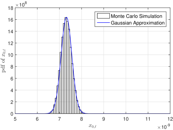
(a) Typical AP

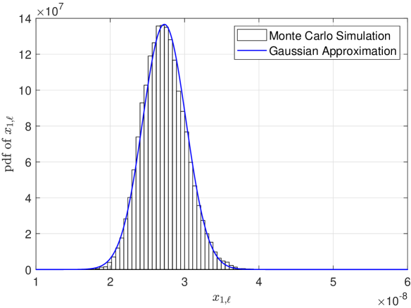
(b) AP $1$

Figure 4: Comparison between the p.d.f. of $x_{j,\ell}$ and its corresponding Gaussian approximation. $R=200$, $\lambda=0.0005$ and $\alpha=4$.

IV-B2 Joint MAP Estimation

Based on the conditional distribution of $\overline{\mathbf{Y}}_{0}$ given $\overline{\mathbf{a}}_{0}$ and $\overline{\mathbf{x}}_{0}$ and the distributions of $\mathbf{a}_{j}$ and $\mathbf{x}_{j}$, $j\in\{0,1,\cdots,6\}$, the conditional joint density of of $\overline{\mathbf{a}}_{0}$ and $\overline{\mathbf{x}}_{0}$, given $\overline{\mathbf{Y}}_{0}$, is given by

$${\color[rgb]{0,0,0}\overline{f}_{\overline{\mathbf{a}}_{0},\overline{\mathbf{x}}_{0}|\overline{\mathbf{Y}}_{0}}\left(\overline{\mathbf{a}}_{0},\overline{\mathbf{x}}_{0},\overline{\mathbf{Y}}_{0}\right)\propto\overline{f}_{\overline{\mathbf{a}}_{0},\overline{\mathbf{x}}_{0}}\left(\overline{\mathbf{Y}}_{0}\right)}\left(\prod_{j=0}^{6}p_{j}(\mathbf{a}_{j})\right)\left(\prod_{j=0}^{6}g_{j}(\mathbf{x}_{j})\right)$$

$$\propto\frac{\exp\left(-\sum\limits_{j=0}^{6}{\rm tr}\left(\left(\overline{\mathbf{P}}_{0}\overline{\mathbf{A}}_{0}\overline{\bm{\Gamma}}_{j}\overline{\mathbf{P}}_{0}^{H}+\mathbf{X}_{j}+\delta^{2}\mathbf{I}_{L}\right)^{-1}\mathbf{Y}_{j}\mathbf{Y}_{j}^{H}\right)\right)}{\prod_{j=0}^{6}|(\overline{\mathbf{P}}_{0}\overline{\mathbf{A}}_{0}\overline{\bm{\Gamma}}_{j}\overline{\mathbf{P}}_{0}^{H}+\mathbf{X}_{j}+\delta^{2}\mathbf{I}_{L})|^{M}}\exp\left(-\sum\limits_{j=0}^{6}\sum\limits_{\ell=1}^{L}\frac{(x_{j,\ell}-\mu_{j})^{2}}{2\sigma_{j}^{2}}\right)$$

$$\quad\times\exp\left(\sum_{j=0}^{6}\sum_{\omega\in\Psi_{j}}\left(c_{\omega}\prod_{i\in\omega}a_{i}\right)\right).$$

The maximization of the conditional joint density $\overline{f}_{\overline{\mathbf{a}}_{0},\overline{\mathbf{x}}_{0}|\overline{\mathbf{Y}}_{0}}\left(\overline{\mathbf{a}}_{0},\overline{\mathbf{x}}_{0},\overline{\mathbf{Y}}_{0}\right)$ is equivalent to the minimization of the negative logarithm of the conditional joint density $-\log{\color[rgb]{0,0,0}\overline{f}_{\overline{\mathbf{a}}_{0},\overline{\mathbf{x}}_{0}|\overline{\mathbf{Y}}_{0}}\left(\overline{\mathbf{a}}_{0},\overline{\mathbf{x}}_{0},\overline{\mathbf{Y}}_{0}\right)}\propto\overline{f}_{\rm MAP}(\overline{\mathbf{a}}_{0},\overline{\mathbf{x}}_{0})$, where

$$\overline{f}_{\rm MAP}(\overline{\mathbf{a}}_{0},\overline{\mathbf{x}}_{0})\triangleq\overline{f}_{\rm ML}(\overline{\mathbf{a}}_{0},\overline{\mathbf{x}}_{0})+\frac{1}{M}\sum_{j=0}^{6}\sum_{\ell=1}^{L}\frac{(x_{j,\ell}-\mu_{j})^{2}}{2\sigma_{j}^{2}}-\frac{1}{M}\sum_{j=0}^{6}\sum_{\omega\in\Psi_{j}}\left(c_{\omega}\prod\limits_{i\in\omega}a_{i}\right).$$

Note that $\frac{1}{M}\sum_{j=0}^{6}\sum_{\ell=1}^{L}\frac{(x_{j,\ell}-\mu_{j})^{2}}{2\sigma_{j}^{2}}$ is from the p.d.f. of $\overline{\mathbf{x}}_{0}$, and $-\frac{1}{M}\sum_{j=0}^{6}\sum_{\omega\in\Psi_{j}}(c_{\omega}\prod_{i\in\omega}a_{i})$ is from the p.m.f. of $\overline{\mathbf{a}}_{0}$. The joint MAP estimate of $\overline{\mathbf{a}}_{0}$ and $\overline{\mathbf{x}}_{0}$ with AP cooperation can be formulated as follows.

Problem 4 (Joint MAP Estimation with AP Cooperation)

$$\min_{\overline{\mathbf{a}}_{0},\overline{\mathbf{x}}_{0}} \quad\overline{f}_{\rm MAP}(\overline{\mathbf{a}}_{0},\overline{\mathbf{x}}_{0})$$

$$s.t. \quad\eqref{eqn:coop_cstrt_a},\eqref{eqn:coop_cstrt_x}.$$

Let $(\overline{\mathbf{a}}_{0}^{\dagger},\overline{\mathbf{x}}_{0}^{\dagger})$ denote an optimal solution of Problem 4.

By comparing $\overline{f}_{\rm MAP}(\overline{\mathbf{a}}_{0},\overline{\mathbf{x}}_{0})$ with $\overline{f}_{\rm ML}(\overline{\mathbf{a}}_{0},\overline{\mathbf{x}}_{0})$, we can draw the following conclusions. The incorporating of prior distribution $g_{j}(\mathbf{x}_{j})$ pushes the estimate of $x_{j,\ell}$ towards its mean $\mu_{j}$ for all $\ell\in\mathcal{L}$. Incorporating prior distribution $p_{j}(\mathbf{a}_{j})$ pushes the estimate of $a_{i}$, $i\in\Phi_{j}$ to the activity states with high probabilities. As $\overline{f}_{\rm MAP}(\overline{\mathbf{a}}_{0},\overline{\mathbf{x}}_{0})-\overline{f}_{\rm ML}(\overline{\mathbf{a}}_{0},\overline{\mathbf{x}}_{0})$ decreases with $M$, the impacts of the prior distributions of $\overline{\mathbf{a}}_{0}$ and $\overline{\mathbf{x}}_{0}$ reduce as $M$ increases. As $M\to\infty$, $\overline{f}_{\rm MAP}(\overline{\mathbf{a}}_{0},\overline{\mathbf{x}}_{0})\to\overline{f}_{\rm ML}(\overline{\mathbf{a}}_{0},\overline{\mathbf{x}}_{0})$, Problem 4 reduces to Problem 3, and $(\overline{\mathbf{a}}_{0}^{\dagger},\overline{\mathbf{x}}_{0}^{\dagger})$ becomes $(\overline{\mathbf{a}}_{0}^{*},\overline{\mathbf{x}}_{0}^{*})$.

As $\overline{f}_{\rm ML}(\overline{\mathbf{a}}_{0},\overline{\mathbf{x}}_{0})$ is a DC function and $-\frac{1}{M}\sum_{j=0}^{6}\sum_{\omega\in\Psi_{j}}\left(c_{\omega}\prod\limits_{i\in\omega}a_{i}\right)$ is a non-convex function, we can see that Problem 4 is a challenging non-convex problem with a complicated objective function. We adopt the coordinate descent method to obtain a stationary point of Problem 4. Specifically, given $\overline{\mathbf{a}}_{0}$ and $\overline{\mathbf{x}}_{0}$ obtained in the previous step, the coordinate descent optimization with respect to $a_{i}$ is equivalent to the optimization of the increment $d$ in $a_{i}$:

$$\min_{1-a_{i}\geq d\geq-a_{i}}\ \overline{f}_{\rm MAP}(\overline{\mathbf{a}}_{0}+d\mathbf{e}_{i},\overline{\mathbf{x}}),$$ (29)

and the coordinate descent optimization with respect to $x_{j,\ell}$ is equivalent to the optimization of the increment $d$ in $x_{j,\ell}$:

$$\min_{d\geq-x_{j,\ell}}\ \overline{f}_{{\rm ML},j}(\overline{\mathbf{a}}_{0},\mathbf{x}_{j}+d\mathbf{e}_{\ell})+\frac{(x_{j,\ell}-\mu_{j}+d)^{2}}{2M\sigma_{j}^{2}}.$$ (30)

Define

$$\widetilde{f}_{a,i}(d,\overline{\mathbf{a}}_{0},\overline{\mathbf{x}}_{0})\triangleq\overline{f}_{a,i}(d,\overline{\mathbf{a}}_{0},\overline{\mathbf{x}}_{0})-\frac{d}{M}\sum_{j=0}^{6}\sum_{\omega\in\Psi_{j}:i\in\omega}\left(c_{\omega}\prod_{i^{{}^{\prime}}\in\omega,i^{{}^{\prime}}\neq i}a_{i^{{}^{\prime}}}\right),$$

$$\widetilde{f}_{x,j,\ell}(d,\overline{\mathbf{a}}_{0},\overline{\mathbf{x}}_{0})\triangleq\log(1+d\mathbf{e}_{\ell}^{H}\mathbf{\Sigma}_{j}^{-1}\mathbf{e}_{\ell})-\frac{d\mathbf{e}_{\ell}^{H}\mathbf{\Sigma}_{j}^{-1}\widehat{\mathbf{\Sigma}}_{\mathbf{Y}_{j}}\mathbf{\Sigma}_{j}^{-1}\mathbf{e}_{\ell}}{1+d\mathbf{e}_{\ell}^{H}\mathbf{\Sigma}_{j}^{-1}\mathbf{e}_{\ell}}+\frac{(x_{j,\ell}-\mu_{j}+d)^{2}}{2M\sigma_{j}^{2}},$$

$$\widetilde{h}_{a,i}(d,\overline{\mathbf{a}}_{0},\overline{\mathbf{x}}_{0})\triangleq\overline{h}_{a,i}(d,\overline{\mathbf{a}}_{0},\overline{\mathbf{x}}_{0})-\frac{1}{M}\sum_{j=0}^{6}\sum_{\omega\in\Psi_{j}:i\in\omega}\left(c_{\omega}\prod_{i^{{}^{\prime}}\in\omega,i^{{}^{\prime}}\neq i}a_{i^{{}^{\prime}}}\right),$$

$$\widetilde{h}_{x,j,\ell}(d,\overline{\mathbf{a}}_{0},\overline{\mathbf{x}}_{0})\triangleq\frac{\mathbf{e}_{\ell}^{H}\mathbf{\Sigma}_{j}^{-1}\mathbf{e}_{\ell}}{1+d\mathbf{e}_{\ell}^{H}\mathbf{\Sigma}_{j}^{-1}\mathbf{e}_{\ell}}-\frac{\mathbf{e}_{\ell}^{H}\mathbf{\Sigma}_{j}^{-1}\widehat{\mathbf{\Sigma}}_{\mathbf{Y}_{j}}\mathbf{\Sigma}_{j}^{-1}\mathbf{e}_{\ell}}{(1+d\mathbf{e}_{\ell}^{H}\mathbf{\Sigma}_{j}^{-1}\mathbf{e}_{\ell})^{2}}+\frac{d+x_{j,\ell}-\mu_{j}}{M\sigma_{j}^{2}}.$$

We write $\widetilde{f}_{a,i}(d,\overline{\mathbf{a}}_{0},\overline{\mathbf{x}}_{0})$, $\widetilde{f}_{x,j,\ell}(d,\overline{\mathbf{a}}_{0},\overline{\mathbf{x}}_{0})$, $\widetilde{h}_{a,i}(d,\overline{\mathbf{a}}_{0},\overline{\mathbf{x}}_{0})$, and $\widetilde{h}_{x,j,\ell}(d,\overline{\mathbf{a}}_{0},\overline{\mathbf{x}}_{0})$ as functions of $\overline{\mathbf{a}}_{0}$ and $\overline{\mathbf{x}}_{0}$, as $\mathbf{\Sigma}_{j}$, $j\in\{0,1,\cdots,6\}$ are functions of $\overline{\mathbf{a}}_{0}$ and ${\mathbf{x}}_{j}$. Note that $\widetilde{h}_{a,i}(d,\overline{\mathbf{a}}_{0},\overline{\mathbf{x}}_{0})$ and $\widetilde{h}_{x,j,\ell}(d,\overline{\mathbf{a}}_{0},\overline{\mathbf{x}}_{0})$ are the derivative functions of $\widetilde{f}_{a,i}(d,\overline{\mathbf{a}}_{0},\overline{\mathbf{x}}_{0})$ and $\widetilde{f}_{x,j,\ell}(d,\overline{\mathbf{a}}_{0},\overline{\mathbf{x}}_{0})$ with respect to $d$, respectively. Denote $\widetilde{\mathcal{A}}_{i}(\overline{\mathbf{a}}_{0},\overline{\mathbf{x}}_{0})\triangleq\{d\in[-a_{i},1-a_{i}]:\widetilde{h}_{a,i}(d,\overline{\mathbf{a}}_{0},\overline{\mathbf{x}}_{0})=0\}$ as the set of roots of equation $\widetilde{h}_{a,i}(d,\overline{\mathbf{a}}_{0},\overline{\mathbf{x}}_{0})=0$ that lie in $[-a_{i},1-a_{i}]$, for given $\overline{\mathbf{a}}_{0}$ and $\overline{\mathbf{x}}_{0}$. Denote $\widetilde{\mathcal{X}}_{j,\ell}(\overline{\mathbf{a}}_{0},\overline{\mathbf{x}}_{0})\triangleq\{d>-x_{j,\ell}:\widetilde{h}_{x,j,\ell}(d,\overline{\mathbf{a}}_{0},\overline{\mathbf{x}}_{0})=0\}$ as the set of roots of equation $\widetilde{h}_{x,j,\ell}(d,\overline{\mathbf{a}}_{0},\overline{\mathbf{x}}_{0})=0$ that are no smaller than $-x_{j,\ell}$, for given $\overline{\mathbf{a}}_{0}$ and $\overline{\mathbf{x}}_{0}$. Based on the structure properties of the coordinate optimization problems in (29) and (30), we have the following results.

Theorem 4 (Optimal Solutions of Coordinate Descent Optimizations in (29) and (30))

Given $\overline{\mathbf{a}}_{0}$ and $\overline{\mathbf{x}}_{0}$ obtained in the previous step, the optimal solution to the coordinate optimization with respect to the increment in $a_{i}$ in (29) is given by

$$\mathop{\arg\min}\limits_{d\in\widetilde{\mathcal{A}}_{i}(\overline{\mathbf{a}}_{0},\overline{\mathbf{x}}_{0})\cup\{-a_{i},1-a_{i}\}}\widetilde{f}_{a,i}(d,\overline{\mathbf{a}}_{0},\overline{\mathbf{x}}_{0}),$$ (31)

and the optimal solution to the coordinate optimization with respect to the increment in $x_{j,\ell}$ in (30) is given by

$$\mathop{\arg\min}\limits_{d\in\widetilde{\mathcal{X}}_{j,\ell}(\overline{\mathbf{a}}_{0},\overline{\mathbf{x}}_{0})\cup\{-x_{j,\ell}\}}\widetilde{f}_{x,j,\ell}(d,\overline{\mathbf{a}}_{0},\overline{\mathbf{x}}_{0}).$$ (32)

Proof:

Theorem 4 can be proved in a similar way to Theorem 2. The details are omitted due to page limitation. ∎

The roots of equation $\widetilde{h}_{a,i}(d,\overline{\mathbf{a}}_{0},\overline{\mathbf{x}}_{0})=0$ can be obtained by solving a univariate polynomial equation of degree 14 using mathematical tools, e.g., MATLAB. The roots of equation $\widetilde{h}_{x,j,\ell}(d,\overline{\mathbf{a}}_{0},\overline{\mathbf{x}}_{0})=0$ can be obtained by solving a cubic equation with one variable, which has closed-form solutions. From Theorem 4, we can see that in the coordinate descent optimizations, prior information on $\overline{\mathbf{a}}_{0}$ and $\overline{\mathbf{x}}_{0}$ affects the updates of $a_{i}$, $i\in\overline{\Phi}_{0}$ and $x_{j,\ell}$, $j\in\{0,1,\cdots,6\}$, $\ell\in\mathcal{L}$, respectively. The details of the coordinate descent algorithm for solving Problem 4 are also summarized in Algorithm 2. As shown in Table I, the computational complexities for solving the coordinate optimizations in (29) and (30) per iteration are higher than those for solving the coordinate optimizations in (24) and (25), as the objective functions incorporating the prior distributions of $\overline{\mathbf{a}}_{0}$ and $\overline{\mathbf{x}}_{0}$ are more complex. Similarly, as $\overline{f}_{\rm MAP}(\overline{\mathbf{a}}_{0},\overline{\mathbf{x}}_{0})$ is continuously differentiable, we can obtain a stationary point of Problem 4 by Algorithm 2 for the joint MAP estimation under a mild condition that each of the coordinate optimizations in (29) and (30) has a unique optimal solution [29, Proposition 2.7.1].

V Numerical Results

In this section, we evaluate the performance of the proposed activity detection designs via numerical results. We compare the proposed designs with four state-of-the-art designs, i.e., AMP (non-cooperative) in [9, 14], ML, and Group-Lasso in [17], which do not consider inter-cell interference or AP cooperation, and AMP (cooperative) in [16] which considers inter-cell interference and AP cooperation. Note that the proposed designs, ML, and Group-Lasso are optimization-based device activity detection designs, and the computational complexities of ML and Group-Lasso per iteration are $\mathcal{O}(N_{0}L^{2})$. AMP (non-cooperative) and AMP (cooperative) are based on the AMP algorithm with the minimum mean squared error (MMSE) denoiser, and their computational complexities per iteration are $\mathcal{O}(N_{0}LM)$. ML has been recognized as the best design among all existing designs in most cases, and the AMP-based designs are also treated as very competitive designs among existing ones.

In the simulation, $N_{0}$ devices are uniformly distributed in cell $0$, and the active devices out of cell $0$ are distributed according to a homogeneous PPP with density $\lambda$. The number of devices in cell $0$ $N_{0}$ is deterministic, and the number of active devices in any other cell is random and has average $\frac{3\sqrt{3}}{2}R^{2}\lambda$. We treat the devices in cell $0$ and outside of it differently for the purpose of separating the impacts of $N_{0}$ and the intensity of inter-cell interference. We assume that each device is active with probability $p_{a}$. We independently generate $2000$ realizations for the locations of devices, $\mathbf{p}_{i}$, $i\in\mathcal{I}$, $a_{i}$, $i\in\mathcal{I}$, and $\mathbf{h}_{i,j}$, $i\in\mathcal{I}$, $j\in\{0,1,\cdots,6\}$, perform device activity detection in each realization, and evaluate the average error probability over all $2000$ realizations. For the proposed designs, ML, and Group-Lasso, let $\hat{a}_{i}\triangleq\mathbf{1}[a_{i}^{*}\geq\theta]$ denote the estimate of the activity state of device $i$, where $\mathbf{1}[\cdot]$ is the indicator function, and $\theta>0$ is a threshold. As $a_{i}\in[0,1]$, the threshold $\theta$ should be chosen from $[0,1]$. It is obvious that the error probability is $1-p_{a}$ when $\theta\leq 0$ and is $p_{a}$ when $\theta\geq 1$. For each of the proposed designs, ML, and Group-Lasso, we evaluate the average error probability for $\theta\in\{0.01,0.02,\cdots,{\color[rgb]{0,0,0}1}\}$ and choose the optimal threshold, i.e., the one achieving the minimum as its average error probability. For AMP (non-cooperative) and AMP (cooperative), let $\hat{a}_{i}\triangleq\mathbf{1}[{\rm LLR}_{i}\geq 0]$ denote the estimate of the activity state of device $i$ [9], where ${\rm LLR}_{i}$ is the log-likelihood ratio for device $i$ and is given by [16, Eq. (13)] and [16, Eq. (15)] for AMP (non-cooperative) and AMP (cooperative), respectively. A detection error happens when $\hat{a}_{i}\neq a_{i}$. In the simulation, unless otherwise stated, we choose $R=200$, $\lambda=0.00025$, $p_{a}=0.05$, $N_{0}=500$, $\alpha=3$, $L=40$, $M=60$ and $\delta^{2}=\frac{R^{-\alpha}}{10}$.

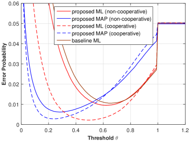
Figure 5: Error probability versus threshold $\theta$ in the i.i.d. case.

Fig. 5 plots the error probabilities of the proposed ML (non-cooperative), proposed MAP (non-cooperative), proposed ML (cooperative), proposed MAP (cooperative), and ML versus the threshold $\theta$. Note that when $\theta$ increases, more devices are detected as inactive. From Fig. 5, we can see that the error probability of each detection design first decreases with $\theta$ due to the decrease of false alarm and then increases with $\theta$ due to the increase of missed detection. In addition, we observe that the optimal thresholds corresponding to the minimum error probabilities for the MAP-based detection designs are smaller than those for the corresponding ML-based detection designs. This is because the incorporation of the prior distribution of device activities (e.g., $p_{a}=0.05$ in the i.i.d. case) makes the estimated activity states of most devices under the MAP-based detection designs smaller than those under the ML-based detection designs.

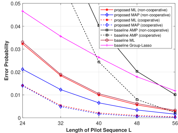
(a) Length of pilot sequences $L$.

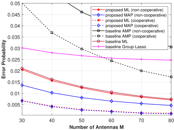
(b) Number of antennas $M$.

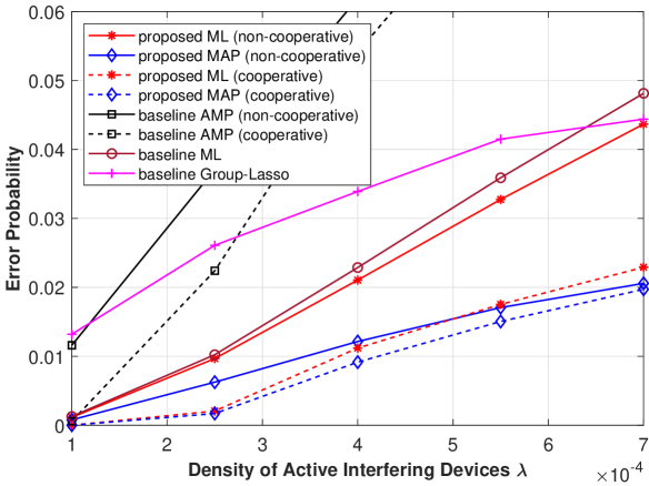
(c) Density of active devices out of typical cell $\lambda$.

Figure 6: Error probability versus length of pilot sequences $L$, number of antennas $M$ and density of active devices out of typical cell $\lambda$ in the i.i.d. case.

Fig. 6 plots the error probability versus the length of pilot sequences $L$, the number of antennas $M$, and the density of active devices outside cell $0$ $\lambda$ in the i.i.d. case, where the devices activate in an i.i.d. manner. From Fig. 6, we observe that the proposed designs outperform the AMP-based designs and Group-Lasso (the error probability of the proposed MAP (non-cooperative) is smaller than $\frac{1}{5}$ of that of AMP (non-cooperative), and the error probability of the proposed MAP (cooperative) is about $\frac{1}{10}$ of that of AMP (cooperative)); the proposed ML (non-cooperative) outperforms ML, especially in the high interference regime; the proposed MAP (non-cooperative) can reduce the error probability by nearly a half, compared to the proposed ML (non-cooperative); the proposed cooperative designs significantly outperform their respective non-cooperative counterparts; the performance of the proposed MAP (cooperative) is similar to that of the proposed ML (cooperative). Note that the performance gain of the proposed ML (non-cooperative) over ML comes from the explicit consideration of inter-cell interference; the performance gain of the proposed MAP (non-cooperative) over the proposed ML (non-cooperative) derives from the incorporation of prior knowledge of the interference powers and device activities; the performance gain of each proposed cooperative design over its non-cooperative counterpart is due to the exploitation of more observations from neighbor APs and the utilization of more network parameters; similar performance of the proposed cooperative designs indicates that exploiting prior knowledge of the interference powers and device activities brings a relatively small gain under AP cooperation. Specifically, from Fig. 6 (a) and (b), we observe that the error probability of each design decreases with $L$ and $M$; and the gap between the proposed MAP (non-cooperative) and the proposed ML (non-cooperative) increases as $L$ and $M$ decrease, which highlights the benefit of prior information at small $L$ and $M$ under non-cooperative device activity detection. From Fig. 6 (c), we can see that the error probability of each design increases with $\lambda$, demonstrating the influence of inter-cell interference in device activity detection. In addition, we can see that the gap between the proposed MAP (non-cooperative) and the proposed ML (non-cooperative) increases with $\lambda$, which shows that the value of prior knowledge of the interference powers increases with their strengths under non-cooperative device activity detection.

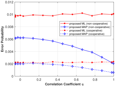
Figure 7: Error probability versus correlation coefficient $\eta$ in the 1st instance in Section III-B1

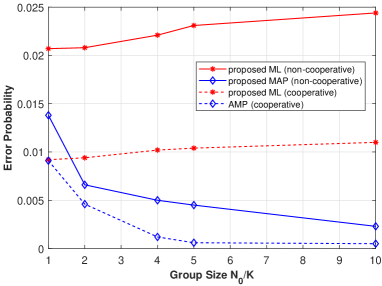
Figure 8: Error probability versus group size $\frac{N_{0}}{K}$ in the 2nd instance in Section III-B1. $|\mathcal{G}_{1}|=\cdots=|\mathcal{G}_{K}|$, $L=30$, and $N_{0}=N_{1}=\cdots=N_{6}$.

Fig. 8 plots the error probability of each proposed design versus the correlation coefficient $\eta$ in the group activity case given by the first instance in Section III-B1. As the baseline designs cannot exploit general sparsity patterns of device activities, we do not show their error probabilities in Fig. 8 and Fig. 8. From Fig. 8, we can observe that the error probabilities of the proposed MAP (non-cooperative) and the proposed MAP (cooperative) decrease with $\eta$, whereas the error probabilities of the other designs nearly do not change with $\eta$. In addition, the error probabilities of the proposed MAP (non-cooperative) and the proposed MAP (cooperative) at $\eta=1$ reduce to about $1/3$ of the corresponding ones at $\eta=0$, which demonstrates the value of exploiting correlation among device activities.

Fig. 8 plots the error probability versus the group size $\frac{N_{0}}{K}$ in the group activity case given by the second instance in Section III-B1. From Fig. 8, we can see that the error probabilities of the proposed ML (non-cooperative) and the proposed ML (cooperative) increase with $\frac{N_{0}}{K}$, as the device activity detection is more challenging when the number of active devices is larger, and the correlation among device activities is not utilized. In contrast, the error probabilities of the proposed MAP (non-cooperative) and the proposed MAP (cooperative) decrease with $\frac{N_{0}}{K}$, as the exploitation of correlation successfully narrows down the set of possible activity states. Note that in the second instance in Section III-B1, when the group size $\frac{N_{0}}{K}$ increases, the variance of the number of active devices in each cell increases, the probability of having a larger number of active devices increases, and the sample space of device activities becomes smaller.

VI Conclusion

This paper considered non-cooperative and cooperative device activity detection in grant-free massive access in a multi-cell network with interfering devices. Under each activity detection mechanism, we formulated the problems for the joint ML estimation and joint MAP estimation of both the device activities and interference powers. Furthermore, for each challenging non-convex problem, we proposed a coordinate descent algorithm to obtain a stationary point. Both analytical and numerical results demonstrated the importance of explicit consideration of inter-cell interference, the values of prior information and network parameters, and the advantage of AP cooperation in device activity detection. To our knowledge, this is the first time that techniques from probability, stochastic geometry, and optimization are jointly utilized in device activity detection for grant-free massive access. Furthermore, this is the first work that considers joint estimation of the device activities and interference powers to improve the accuracy of device activity detection.

Appendix A: Proof of Theorem 1

First, consider the coordinate optimization with respect to $a_{i}$. By (4), we have

$$f_{\rm ML}(\mathbf{a}_{0}+d\mathbf{e}_{i},\mathbf{x})\stackrel{{\scriptstyle(a)}}{{=}}\log|\mathbf{\Sigma}+d\gamma_{i,0}\mathbf{p}_{i}\mathbf{p}_{i}^{H}|+{\rm tr}((\mathbf{\Sigma}+d\gamma_{i,0}\mathbf{p}_{i}\mathbf{p}_{i}^{H})^{-1}\widehat{\mathbf{\Sigma}}_{\mathbf{Y}_{0}})$$

$$\stackrel{{\scriptstyle(b)}}{{=}}\log\left(|\mathbf{\Sigma}|(1+d\gamma_{i,0}\mathbf{p}_{i}^{H}\mathbf{\Sigma}^{-1}\mathbf{p}_{i})\right)+{\rm tr}\left(\left(\mathbf{\Sigma}^{-1}-\frac{d\gamma_{i,0}\mathbf{\Sigma}^{-1}\mathbf{p}_{i}\mathbf{p}_{i}^{H}\mathbf{\Sigma}^{-1}}{1+d\gamma_{i,0}\mathbf{p}_{i}^{H}\mathbf{\Sigma}^{-1}\mathbf{p}_{i}}\right)\widehat{\mathbf{\Sigma}}_{\mathbf{Y}_{0}}\right)$$

$${\color[rgb]{0,0,0}\stackrel{{\scriptstyle(c)}}{{=}}}f_{\rm ML}(\mathbf{a}_{0},\mathbf{x})+\log\left(1+d\gamma_{i,0}\mathbf{p}_{i}^{H}\mathbf{\Sigma}^{-1}\mathbf{p}_{i}\right)-\frac{d\gamma_{i,0}\mathbf{p}_{i}^{H}\mathbf{\Sigma}^{-1}\widehat{\mathbf{\Sigma}}_{\mathbf{Y}_{0}}\mathbf{\Sigma}^{-1}\mathbf{p}_{i}}{1+d\gamma_{i,0}\mathbf{p}_{i}^{H}\mathbf{\Sigma}^{-1}\mathbf{p}_{i}},$$ (33)

where $(a)$ is due to $\mathbf{\Sigma}=\mathbf{P}_{0}\mathbf{A}_{0}\bm{\Gamma}_{0}\mathbf{P}_{0}^{H}+\mathbf{X}+\delta^{2}\mathbf{I}_{L}$ and $\mathbf{P}_{0}\mathbf{A}_{0}\bm{\Gamma}_{0}\mathbf{P}_{0}^{H}=\sum_{i\in\Phi_{0}}a_{i}\gamma_{i,0}\mathbf{p}_{i}\mathbf{p}_{i}^{H}$, (b) is due to the fact that for any positive definite matrix $\mathbf{\Sigma}$, $(\mathbf{\Sigma}+d\gamma_{i,0}\mathbf{p}_{i}\mathbf{p}_{i}^{H})^{-1}=\mathbf{\Sigma}^{-1}-\frac{d\gamma_{i,0}\mathbf{\Sigma}^{-1}\mathbf{p}_{i}\mathbf{p}_{i}^{H}\mathbf{\Sigma}^{-1}}{1+d\gamma_{i,0}\mathbf{p}_{i}^{H}\mathbf{\Sigma}^{-1}\mathbf{p}_{i}}$ and $|\mathbf{\Sigma}+d\gamma_{i,0}\mathbf{p}_{i}\mathbf{p}_{i}^{H}|=|\mathbf{\Sigma}|(1+d\gamma_{i,0}\mathbf{p}_{i}^{H}\mathbf{\Sigma}^{-1}\mathbf{p}_{i})$ hold [17], and (c) is due to the cyclic property of trace. Note that $f_{\rm ML}(\mathbf{a}_{0}+d\mathbf{e}_{i},\mathbf{x})$ is well-defined only when $d>d_{0}\triangleq-\frac{1}{\gamma_{i,0}\mathbf{p}_{i}^{H}\mathbf{\Sigma}^{-1}\mathbf{p}_{i}}$. By (33), we have

$$\frac{\partial f_{\rm ML}(\mathbf{a}_{0}+d\mathbf{e}_{i},\mathbf{x})}{\partial d}=\frac{\gamma_{i,0}\mathbf{p}_{i}^{H}\mathbf{\Sigma}^{-1}\mathbf{p}_{i}}{1+d\gamma_{i,0}\mathbf{p}_{i}^{H}\mathbf{\Sigma}^{-1}\mathbf{p}_{i}}-\frac{\gamma_{i,0}\mathbf{p}_{i}^{H}\mathbf{\Sigma}^{-1}\widehat{\mathbf{\Sigma}}_{\mathbf{Y}_{0}}\mathbf{\Sigma}^{-1}\mathbf{p}_{i}}{(1+d\gamma_{i,0}\mathbf{p}_{i}^{H}\mathbf{\Sigma}^{-1}\mathbf{p}_{i})^{2}}.$$ (34)

Thus, the solution of $\frac{\partial f_{\rm ML}(\mathbf{a}+d\mathbf{e}_{i},\mathbf{x})}{\partial d}=0$ is $d_{a}^{*}\triangleq\frac{\mathbf{p}_{i}^{H}\mathbf{\Sigma}^{-1}\widehat{\mathbf{\Sigma}}_{\mathbf{Y}_{0}}\mathbf{\Sigma}^{-1}\mathbf{p}_{i}-\mathbf{p}_{i}^{H}\mathbf{\Sigma}^{-1}\mathbf{p}_{i}}{\gamma_{i,0}(\mathbf{p}_{i}^{H}\mathbf{\Sigma}^{-1}\mathbf{p}_{i})^{2}}$. As $\widehat{\mathbf{\Sigma}}_{\mathbf{Y}_{0}}=\frac{1}{M}\mathbf{Y}_{0}\mathbf{Y}_{0}^{H}$ and $\mathbf{\Sigma}$ is a Hermitian matrix, we have $\mathbf{p}_{i}^{H}\mathbf{\Sigma}^{-1}\widehat{\mathbf{\Sigma}}_{\mathbf{Y}_{0}}\mathbf{\Sigma}^{-1}\mathbf{p}_{i}\geq 0$ and $d_{a}^{*}\geq-\frac{1}{\gamma_{i,0}\mathbf{p}_{i}^{H}\mathbf{\Sigma}^{-1}\mathbf{p}_{i}}$. In addition, we note that $\lim_{\epsilon\to 0^{+}}f_{\rm ML}(\mathbf{a}_{0}+(d_{0}+\epsilon)\mathbf{e}_{i},\mathbf{x})=+\infty$ and $\lim_{d\to+\infty}f_{\rm ML}(\mathbf{a}_{0}+d\mathbf{e}_{i},\mathbf{x})=+\infty$. Therefore, combining with $a_{i}\in[0,1]$, we can obtain the optimal solution of (7) as in (9).

Next, consider the coordinate optimization with respect to $x_{\ell}$. Similarly, by (4), we have

$$f_{\rm ML}(\mathbf{a}_{0},\mathbf{x}+d\mathbf{e}_{\ell})=\log|\mathbf{\Sigma}+d\mathbf{e}_{\ell}\mathbf{e}_{\ell}^{H}|+{\rm tr}((\mathbf{\Sigma}+d\mathbf{e}_{\ell}\mathbf{e}_{\ell}^{H})^{-1}\widehat{\mathbf{\Sigma}}_{\mathbf{Y}_{0}})$$

$$=\log\left(|\mathbf{\Sigma}|(1+d\mathbf{e}_{\ell}^{H}\mathbf{\Sigma}^{-1}\mathbf{e}_{\ell})\right)+{\rm tr}\left(\left(\mathbf{\Sigma}^{-1}-\frac{d\mathbf{\Sigma}^{-1}\mathbf{e}_{\ell}\mathbf{e}_{\ell}^{H}\mathbf{\Sigma}^{-1}}{1+d\mathbf{e}_{\ell}^{H}\mathbf{\Sigma}^{-1}\mathbf{e}_{\ell}}\right)\widehat{\mathbf{\Sigma}}_{\mathbf{Y}_{0}}\right)$$

$$=f_{\rm ML}(\mathbf{a}_{0},\mathbf{x})+\log\left(1+d\mathbf{e}_{\ell}^{H}\mathbf{\Sigma}^{-1}\mathbf{e}_{\ell}\right)-\frac{d\mathbf{e}_{\ell}^{H}\mathbf{\Sigma}^{-1}\widehat{\mathbf{\Sigma}}_{\mathbf{Y}_{0}}\mathbf{\Sigma}^{-1}\mathbf{e}_{\ell}}{1+d\mathbf{e}_{\ell}^{H}\mathbf{\Sigma}^{-1}\mathbf{e}_{\ell}},$$ (35)

By (35), we have

$$\frac{\partial f_{\rm ML}(\mathbf{a}_{0},\mathbf{x}+d\mathbf{e}_{\ell})}{\partial d}=\frac{\mathbf{e}_{\ell}^{H}\mathbf{\Sigma}^{-1}\mathbf{e}_{\ell}}{1+d\mathbf{e}_{\ell}^{H}\mathbf{\Sigma}^{-1}\mathbf{e}_{\ell}}-\frac{\mathbf{e}_{\ell}^{H}\mathbf{\Sigma}^{-1}\widehat{\mathbf{\Sigma}}_{\mathbf{Y}_{0}}\mathbf{\Sigma}^{-1}\mathbf{e}_{\ell}}{(1+d\mathbf{e}_{\ell}^{H}\mathbf{\Sigma}^{-1}\mathbf{e}_{\ell})^{2}}.$$

Thus, the solution of $\frac{\partial f_{\rm ML}(\mathbf{a}_{0},\mathbf{x}+d\mathbf{e}_{\ell})}{\partial d}=0$ is $d_{x}^{*}\triangleq\frac{\mathbf{e}_{\ell}^{H}\mathbf{\Sigma}^{-1}\widehat{\mathbf{\Sigma}}_{\mathbf{Y}_{0}}\mathbf{\Sigma}^{-1}\mathbf{e}_{\ell}-\mathbf{e}_{\ell}^{H}\mathbf{\Sigma}^{-1}\mathbf{e}_{\ell}}{(\mathbf{e}_{\ell}^{H}\mathbf{\Sigma}^{-1}\mathbf{e}_{\ell})^{2}}$. Similarly, combining with $x_{\ell}\geq 0$, we can obtain the optimal solution of (8) as in (10).

Appendix B: Proof of Lemma 1

To show Lemma 1, it is sufficient to calculate the mean and variance of $\sum_{i\in\mathcal{I}\setminus\Phi_{0}}a_{i}\gamma_{i,0}$. Let $\mathcal{I}_{t}$ denote the set of indices of the active interfering devices out of the typical cell. Recall that the locations of active interfering devices follow a homogeneous PPP with density $\lambda$. According to Campbell’s theorem for sums, we have

$${\color[rgb]{0,0,0}\mu=}\mathbb{E}\left[\sum_{i\in\mathcal{I}\setminus\Phi_{0}}a_{i}\gamma_{i,0}\right] =\mathbb{E}\left[\sum_{i\in\mathcal{I}_{t}}d_{i,0}^{-\alpha}\right]=\lambda\int_{\mathbb{R}^{2}\setminus S_{0}}d(t)^{-\alpha}{\rm d}t=12\lambda\int_{\frac{\sqrt{3}}{2}R}^{\infty}\int_{0}^{\frac{\sqrt{3}}{3}x}(x^{2}+y^{2})^{-\frac{\alpha}{2}}{\rm d}y{\rm d}x,$$

where $S_{0}$ denotes the area of the typical cell and $d(t)$ is the distance between point $t$ and the origin. According to the variance result for PPPs in [25, Page 85], we have

$${\color[rgb]{0,0,0}\sigma^{2}=}{\rm var}\left[\sum_{i\in\mathcal{I}\setminus\Phi_{0}}a_{i}\gamma_{i,0}\right] ={\rm var}\left[\sum_{i\in\mathcal{I}_{t}}d_{i,0}^{-\alpha}\right]=\lambda\int_{\mathbb{R}^{2}\setminus S_{0}}d(t)^{-2\alpha}{\rm d}t=12\lambda\int_{\frac{\sqrt{3}}{2}R}^{\infty}\int_{0}^{\frac{\sqrt{3}}{3}x}(x^{2}+y^{2})^{-\alpha}{\rm d}y{\rm d}x.$$

Appendix C: Proof of Theorem 2

First, we consider the coordinate descent optimization with respect to $a_{i}$ in (14). As $f_{\rm MAP}(\mathbf{a}_{0}+d\mathbf{e}_{i},\mathbf{x})=f_{\rm ML}(\mathbf{a}_{0}+d\mathbf{e}_{i},\mathbf{x})-C_{i}d$, we have $\frac{\partial f_{\rm MAP}(\mathbf{a}_{0}+d\mathbf{e}_{i},\mathbf{x})}{\partial d}=\frac{\partial f_{\rm ML}(\mathbf{a}_{0}+d\mathbf{e}_{i},\mathbf{x})}{\partial d}-C_{i}$. By (34), we have

$$\frac{\partial^{2}f_{\rm MAP}(\mathbf{a}_{0}+d\mathbf{e}_{i},\mathbf{x})}{\partial d^{2}} =\frac{\partial^{2}f_{\rm ML}(\mathbf{a}_{0}+d\mathbf{e}_{i},\mathbf{x})}{\partial d^{2}}$$

$$=\frac{\gamma_{i,0}^{2}\mathbf{p}_{i}^{H}\mathbf{\Sigma}^{-1}\mathbf{p}_{i}\left(2\mathbf{p}_{i}^{H}\mathbf{\Sigma}^{-1}\widehat{\mathbf{\Sigma}}_{\mathbf{Y}_{0}}\mathbf{\Sigma}^{-1}\mathbf{p}_{i}-\mathbf{p}_{i}^{H}\mathbf{\Sigma}^{-1}\mathbf{p}_{i}-d\gamma_{i,0}(\mathbf{p}_{i}^{H}\mathbf{\Sigma}^{-1}\mathbf{p}_{i})^{2}\right)}{(1+d\gamma_{i,0}\mathbf{p}_{i}^{H}\mathbf{\Sigma}^{-1}\mathbf{p}_{i})^{3}}.$$

The solution of $\frac{\partial^{2}f_{\rm MAP}(\mathbf{a}_{0}+d\mathbf{e}_{i},\mathbf{x})}{\partial d^{2}}=0$ is $d_{2}\triangleq\frac{2\mathbf{p}_{i}^{H}\mathbf{\Sigma}^{-1}\widehat{\mathbf{\Sigma}}_{\mathbf{Y}_{0}}\mathbf{\Sigma}^{-1}\mathbf{p}_{i}-\mathbf{p}_{i}^{H}\mathbf{\Sigma}^{-1}\mathbf{p}_{i}}{\gamma_{i,0}(\mathbf{p}_{i}^{H}\mathbf{\Sigma}^{-1}\mathbf{p}_{i})^{2}}$. As $\frac{\partial^{2}f_{\rm MAP}(\mathbf{a}_{0}+d\mathbf{e}_{i},\mathbf{x})}{\partial d^{2}}>0$ in $d\in(d_{0},d_{2})$ and $\frac{\partial^{2}f_{\rm MAP}(\mathbf{a}_{0}+d\mathbf{e}_{i},\mathbf{x})}{\partial d^{2}}<0$ in $d\in(d_{2},\infty)$, we know that $\frac{\partial f_{\rm MAP}(\mathbf{a}_{0}+d\mathbf{e}_{i},\mathbf{x})}{\partial d}$ increases with $d$ in $(d_{0},d_{2})$, decreases with $d$ in $(d_{2},\infty)$, and achieves its maximum $\frac{\gamma_{i,0}(\mathbf{p}_{i}^{H}\mathbf{\Sigma}^{-1}\mathbf{p}_{i})^{2}}{4\mathbf{p}_{i}^{H}\mathbf{\Sigma}^{-1}\widehat{\mathbf{\Sigma}}_{\mathbf{Y}_{0}}\mathbf{\Sigma}^{-1}\mathbf{p}_{i}}-C_{i}$ at $d=d_{2}$. As $\lim_{\epsilon\to 0^{+}}\frac{\partial f_{\rm MAP}(\mathbf{a}_{0}+(d_{0}+\epsilon)\mathbf{e}_{i},\mathbf{x})}{\partial d}=-\infty$ and $\lim_{d\to\infty}\frac{\partial f_{\rm MAP}(\mathbf{a}_{0}+d\mathbf{e}_{i},\mathbf{x})}{\partial d}=-C_{i}$, the range of $\frac{\partial f_{\rm MAP}(\mathbf{a}_{0}+d\mathbf{e}_{i},\mathbf{x})}{\partial d}$ is $\left(-\infty,\frac{\gamma_{i,0}(\mathbf{p}_{i}^{H}\mathbf{\Sigma}^{-1}\mathbf{p}_{i})^{2}}{4\mathbf{p}_{i}^{H}\mathbf{\Sigma}^{-1}\widehat{\mathbf{\Sigma}}_{\mathbf{Y}_{0}}\mathbf{\Sigma}^{-1}\mathbf{p}_{i}}-C_{i}\right]$.

Now, we consider the following three cases. When $C_{i}\leq 0$, equation $\frac{\partial f_{\rm MAP}(\mathbf{a}_{0}+d\mathbf{e}_{i},\mathbf{x})}{\partial d}=0$ has one solution $s_{i}(\mathbf{a}_{0},\mathbf{x})\triangleq\frac{1}{2C_{i}}\left(1-\sqrt{1-\frac{4C_{i}\mathbf{p}_{i}^{H}\mathbf{\Sigma}^{-1}\widehat{\mathbf{\Sigma}}_{\mathbf{Y}_{0}}\mathbf{\Sigma}^{-1}\mathbf{p}_{i}}{\gamma_{i}(\mathbf{p}_{i}^{H}\mathbf{\Sigma}^{-1}\mathbf{p}_{i})^{2}}}\right)-\frac{1}{\gamma_{i}\mathbf{p}_{i}^{H}\mathbf{\Sigma}^{-1}\mathbf{p}_{i}}$. We know that $f_{\rm MAP}(\mathbf{a}_{0}+d\mathbf{e}_{i},\mathbf{x})$ decreases with $d$ in $(d_{0},s_{i}(\mathbf{a}_{0},\mathbf{x}))$, increases with $d$ in $(s_{i}(\mathbf{a}_{0},\mathbf{x}),+\infty)$ and achieves its maximum at $d=s_{i}(\mathbf{a}_{0},\mathbf{x})$. Combining with the constraint $a_{i}\in[0,1]$, we have the optimal solution given in (16). When $C_{i}\geq\frac{\gamma_{i,0}(\mathbf{p}_{i}^{H}\mathbf{\Sigma}^{-1}\mathbf{p}_{i})^{2}}{4\mathbf{p}_{i}^{H}\mathbf{\Sigma}^{-1}\widehat{\mathbf{\Sigma}}_{\mathbf{Y}_{0}}\mathbf{\Sigma}^{-1}\mathbf{p}_{i}}$, $f_{\rm MAP}(\mathbf{a}_{0}+d\mathbf{e}_{i},\mathbf{x})$ decreases with $d$ in $(d_{0},+\infty)$. Combining with the constraint $a_{i}\in[0,1]$, we have the optimal solution given in (16). When $0<C_{i}<\frac{\gamma_{i,0}(\mathbf{p}_{i}^{H}\mathbf{\Sigma}^{-1}\mathbf{p}_{i})^{2}}{4\mathbf{p}_{i}^{H}\mathbf{\Sigma}^{-1}\widehat{\mathbf{\Sigma}}_{\mathbf{Y}_{0}}\mathbf{\Sigma}^{-1}\mathbf{p}_{i}}$, equation $\frac{\partial f_{\rm MAP}(\mathbf{a}_{0}+d\mathbf{e}_{i},\mathbf{x})}{\partial d}=0$ has two solutions $s_{i}(\mathbf{a}_{0},\mathbf{x})$ and $\overline{s}_{i}(\mathbf{a}_{0},\mathbf{x})$, where

$$\overline{s}_{i}(\mathbf{a}_{0},\mathbf{x})\triangleq\frac{1}{2C_{i}}\left(1+\sqrt{1-\frac{4C_{i}\mathbf{p}_{i}^{H}\mathbf{\Sigma}^{-1}\widehat{\mathbf{\Sigma}}_{\mathbf{Y}_{0}}\mathbf{\Sigma}^{-1}\mathbf{p}_{i}}{\gamma_{i,0}(\mathbf{p}_{i}^{H}\mathbf{\Sigma}^{-1}\mathbf{p}_{i})^{2}}}\right)-\frac{1}{\gamma_{i,0}\mathbf{p}_{i}^{H}\mathbf{\Sigma}^{-1}\mathbf{p}_{i}}.$$

We know that $f_{\rm MAP}(\mathbf{a}_{0}+d\mathbf{e}_{i},\mathbf{x})$ decreases with $d$ in $(d_{0},s_{i}(\mathbf{a}_{0},\mathbf{x}))$ and $(\overline{s}_{i}(\mathbf{a}_{0},\mathbf{x}),+\infty)$, and increases with $d$ in $(s_{i}(\mathbf{a}_{0},\mathbf{x}),\overline{s}_{i}(\mathbf{a}_{0},\mathbf{x}))$. Combining with the constraint $a_{i}\in[0,1]$, we have the optimal solution given in (16).

Next, we consider the coordinate descent optimization with respect to $x_{\ell}$ in (15). Note that $h_{x,\ell}(d,\mathbf{a}_{0},\mathbf{x})$ is the derivative function of $f_{x,\ell}(d,\mathbf{a}_{0},\mathbf{x})$ with respect to $d$. Combining with the constraint $x_{\ell}>0$, we know that $f_{x,\ell}(d,\mathbf{a}_{0},\mathbf{x})$ achieves its maximum at one point in $\mathcal{X}_{\ell}(\mathbf{a}_{0},\mathbf{x})\cup\{-x_{\ell}\}$, where $\mathcal{X}_{\ell}(\mathbf{a}_{0},\mathbf{x})\triangleq\{d\geq-x_{\ell}:h_{x,\ell}(d,\mathbf{a}_{0},\mathbf{x})=0\}$, which has the optimal objective value. Therefore, we complete the proof.

Appendix D: Proof of Corollary 1

First, we derive $f_{\rm MAP}(\mathbf{a}_{0},\mathbf{x})$ in the i.i.d. case. Note that in the i.i.d. case,

$$p(\mathbf{a}_{0}){\color[rgb]{0,0,0}=\prod_{i\in\Phi_{0}}p_{a}^{a_{i}}(1-p_{a})^{1-a_{i}}}=\exp\left(\log\frac{p_{a}}{1-p_{a}}\sum_{i\in\Phi_{0}}a_{i}+N_{0}\log(1-p_{a})\right).$$

Based on (13), $f_{\rm MAP}(\mathbf{a}_{0},\mathbf{x})$ in the i.i.d. case is given by

$$f_{\rm MAP}(\mathbf{a}_{0},\mathbf{x})=f_{\rm ML}(\mathbf{a}_{0},\mathbf{x})+\frac{1}{2M\sigma^{2}}\sum_{\ell\in\mathcal{L}}(x_{\ell}-\mu)^{2}-\frac{1}{M}\log\frac{p_{a}}{1-p_{a}}\sum_{i\in\overline{\Phi}_{0}}a_{i}.$$ (36)

By (36), we know that $C_{i}=\frac{1}{M}\log\frac{p_{a}}{1-p_{a}}<0$ (as $p_{a}\ll 1$). Substituting $C_{i}=\frac{1}{M}\log\frac{p_{a}}{1-p_{a}}$ into (16), we can obtain the optimal solution of (14) as in (18) in the i.i.d. case.

References

- [1] D. Jiang and Y. Cui, “Ml estimation and map estimation for device activity in grant-free massive access with interference,” in Proc. IEEE WCNC, Apr. 2020, pp. 1–6.
- [2] ——, “Map-based pilot state detection in grant-free random access for mmtc,” in 2020 IEEE 21st International Workshop on Signal Processing Advances in Wireless Communications (SPAWC), 2020, pp. 1–5.
- [3] E. d. Carvalho, E. Bjornson, J. H. Sorensen, P. Popovski, and E. G. Larsson, “Random access protocols for massive mimo,” IEEE Commun. Mag., vol. 55, no. 5, pp. 216–222, May 2017.
- [4] L. Liu, E. G. Larsson, W. Yu, P. Popovski, C. Stefanovic, and E. de Carvalho, “Sparse signal processing for grant-free massive connectivity: A future paradigm for random access protocols in the internet of things,” IEEE Signal Process. Mag., vol. 35, no. 5, pp. 88–99, Sep. 2018.
- [5] C. Bockelmann, N. Pratas, H. Nikopour, K. Au, T. Svensson, C. Stefanovic, P. Popovski, and A. Dekorsy, “Massive machine-type communications in 5g: physical and mac-layer solutions,” IEEE Commun. Mag., vol. 54, no. 9, pp. 59–65, Sep. 2016.
- [6] X. Chen, Z. Zhang, C. Zhong, R. Jia, and D. W. K. Ng, “Fully non-orthogonal communication for massive access,” IEEE Trans. Commun., vol. 66, no. 4, pp. 1717–1731, Apr. 2018.
- [7] K. Senel and E. G. Larsson, “Grant-free massive mtc-enabled massive mimo: A compressive sensing approach,” IEEE Trans. Commun., vol. 66, no. 12, pp. 6164–6175, Dec 2018.
- [8] Z. Chen, F. Sohrabi, Y. Liu, and W. Yu, “Covariance based joint activity and data detection for massive random access with massive mimo,” in Proc. IEEE ICC, May 2019, pp. 1–6.
- [9] L. Liu and W. Yu, “Massive connectivity with massive mimo—part i: Device activity detection and channel estimation,” IEEE Trans. Signal Process., vol. 66, no. 11, pp. 2933–2946, Jun. 2018.
- [10] Y. Cui, S. Li, and W. Zhang, “Jointly sparse signal recovery and support recovery via deep learning with applications in mimo-based grant-free random access,” IEEE Journal on Selected Areas in Communications, pp. 1–1, 2020.
- [11] X. Xu, X. Rao, and V. K. N. Lau, “Active user detection and channel estimation in uplink cran systems,” in Proc. IEEE ICC, Jun. 2015, pp. 2727–2732.
- [12] C. Bockelmann, H. F. Schepker, and A. Dekorsy, “Compressive sensing based multi-user detection for machine-to-machine communication,” Transactions on Emerging Telecommunications Technologies, vol. 24, no. 4, pp. 389–400, 2013.
- [13] Y. Zhang, Q. Guo, Z. Wang, J. Xi, and N. Wu, “Block sparse bayesian learning based joint user activity detection and channel estimation for grant-free noma systems,” IEEE Trans. Veh. Technol., vol. 67, no. 10, pp. 9631–9640, Oct. 2018.
- [14] Z. Chen, F. Sohrabi, and W. Yu, “Sparse activity detection for massive connectivity,” IEEE Trans. Signal Process., vol. 66, no. 7, pp. 1890–1904, April 2018.
- [15] X. Shao, X. Chen, C. Zhong, J. Zhao, and Z. Zhang, “A unified design of massive access for cellular internet of things,” IEEE Internet of Things Journal, vol. 6, no. 2, pp. 3934–3947, Apr. 2019.
- [16] Z. Chen, F. Sohrabi, and W. Yu, “Multi-cell sparse activity detection for massive random access: Massive mimo versus cooperative mimo,” IEEE Trans. Wireless Commun., vol. 18, no. 8, pp. 4060–4074, Aug. 2019.
- [17] S. Haghighatshoar, P. Jung, and G. Caire, “Improved scaling law for activity detection in massive mimo systems,” in Proc. IEEE ISIT, Jun. 2018, pp. 381–385.
- [18] A. Fengler, G. Caire, P. Jung, and S. Haghighatshoar, “Massive MIMO unsourced random access,” CoRR, vol. abs/1901.00828, 2019. [Online]. Available: http://arxiv.org/abs/1901.00828
- [19] Z. Chen and W. Yu, “Phase transition analysis for covariance based massive random access with massive mimo,” in Proc. ASILOMAR, Nov. 2019, pp. 1–5.
- [20] B. Liu, Z. Wei, J. Yuan, and M. Pajovic, “Deep learning assisted user identification in massive machine-type communications,” in Proc. IEEE GLOBECOM, Dec. 2019, pp. 1–6.
- [21] Z. Zhang, Y. Li, C. Huang, Q. Guo, C. Yuen, and Y. L. Guan, “Dnn-aided block sparse bayesian learning for user activity detection and channel estimation in grant-free non-orthogonal random access,” IEEE Trans. Veh. Technol., vol. 68, no. 12, pp. 12 000–12 012, Dec. 2019.
- [22] N. Ye, X. Li, H. Yu, A. Wang, W. Liu, and X. Hou, “Deep learning aided grant-free noma toward reliable low-latency access in tactile internet of things,” IEEE Trans. Ind. Inf., vol. 15, no. 5, pp. 2995–3005, May 2019.
- [23] S. Ding, G. Wahba, and J. Zhu, “Learning higher-order graph structure with features by structure penalty,” in Advances in Neural Information Processing Systems 24. Curran Associates, Inc., 2011, pp. 253–261.
- [24] M. Haenggi and R. K. Ganti, “Interference in large wireless networks,” Foundations and Trends in Networking, vol. 3, no. 2, pp. 127–248, 2009.
- [25] M. Haenggi, Stochastic geometry for wireless networks. Cambridge University Press, 2012.
- [26] J. G. Andrews, F. Baccelli, and R. K. Ganti, “A tractable approach to coverage and rate in cellular networks,” IEEE Trans. Commun., vol. 59, no. 11, pp. 3122–3134, 2011.
- [27] J. G. Andrews, W. Choi, and R. W. Heath, “Overcoming interference in spatial multiplexing mimo cellular networks,” IEEE Wireless Commun., vol. 14, no. 6, pp. 95–104, Dec. 2007.
- [28] J. Choi, “Noma-based compressive random access using gaussian spreading,” IEEE Trans. Commun., vol. 67, no. 7, pp. 5167–5177, Jul. 2019.
- [29] D. Bertsekas, Nonlinear Programming. Athena Scientific, 1999.
- [30] O. Banerjee, L. E. Ghaoui, and A. d’Aspremont, “Model selection through sparse maximum likelihood estimation for multivariate gaussian or binary data,” Journal of Machine learning research, vol. 9, no. Mar, pp. 485–516, 2008.
- [31] M. Aljuaid and H. Yanikomeroglu, “Investigating the gaussian convergence of the distribution of the aggregate interference power in large wireless networks,” IEEE Trans. Veh Technology, vol. 59, no. 9, pp. 4418–4424, Nov. 2010.
- [32] A. Hasan and J. G. Andrews, “The guard zone in wireless ad hoc networks,” IEEE Trans. Wireless Commun., vol. 6, no. 3, pp. 897–906, Mar. 2007.