Sharp-interface limits of the diffuse interface model for two-phase inductionless magnetohydrodynamic fluids

Abstract

In this paper, we propose and analyze a diffuse interface model for inductionless magnetohydrodynamic fluids. The model couples a convective Cahn-Hilliard equation for the evolution of the interface, the Navier–Stokes system for fluid flow and the possion equation for electrostatics. The model is derived from Onsager’s variational principle and conservation laws systematically. We perform formally matched asymptotic expansions and develop several sharp interface models in the limit when the interfacial thickness tends to zero. It is shown that the sharp interface limit of the models are the standard incompressible inductionless magnetohydrodynamic equations coupled with several different interface conditions for different choice of the mobilities. Numerical results verify the convergence of the diffuse interface model with different mobilitiess.

1 Introduction

Incompressible Magnetohydrodynamics (MHD) is the study of the interaction between the conducting incompressible fluid flows and electromagnetic fields. The corresponding model is a system of partial differential equations, which couples the Navier–Stokes equations and the Maxwell equations via Lorentz’s force and Ohm’s Law. However, in most industrial and laboratory flows, MHD flows typically occur at small magnetic Reynolds number. In these situations, the induced magnetic field is usually neglected compared with the applied magnetic field. The MHD equations with this simplification are known as the inductionless MHD model. We refer to [1, 2, 3, 4, 5] for the extensive theoretical modeling, numerical methods and numerical analysis for this model.

In this paper, we focus on the dynamic behavior of two incompressible, immiscible and electrically conducting fluids under the influence of a magnetic field. It has a number of technological and industrial applications such as fusion reactor blankets, metallurgical industry, liquid metal magnetic pumps and aluminum electrolysis [3, 6, 7, 8]. In the process of metallurgy and metal material processing, the two-phase interface problems are involved in the dynamic evolution of air bubbles and in metal liquid, the shaking of the surface of metal liquid in the container and the dynamic behavior of floating or attached metal droplets. In a fusion reactor, two-phase MHD flow is used to describe the laying process in the liquid-metal cooling blanket [1]. Thus, the interfacial dynamic of two-phase MHD problem has been a topic of great interest.

The theoretical analysis and numerical simulation of multi-phase flow is a challenging problem in computational fluid dynamics. A major effort has been made for studying interfacial dynamic problems in the past decades. There are two prevalent approaches to the study of two-phase flows in the literature, sharp interface method and diffuse interface method. The former is built on the assumption that the fluids under investigation are completely immiscible, see Fig. 1.1 for an illustration. Thus, a sharp interface (free curve) that will deform with time exists between the two fluids. This kind of approach usually leads to a model consists of the bulk equations for each phase and a set of interfacial balance conditions. The sharp interface models have been very successful in engineering and scientific applications [9, 10, 11, 12]. In the literature, several numerical methods have been developed to numerically solve the sharp-interface model for the two-phase inductionless MHD flows. Examples of such methods are the front-tracking method [13], the volume-of-fluid method [14, 15], the level-set method [16, 17]. However, there are several known drawbacks associated with this sharp interface approach. In particular, this approach is not able or not be convenient to handle the topological changes such as self-intersection, pinch-off, splitting, and fattening, and moving contact lines.

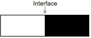
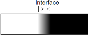
Figure 1.1: Sharp interface(Left) and diffusive interface(Right).

An alternative approach, the so-called diffuse interface or phase-field method is based on the assumption that the macroscopically immiscible fluids are mixed partially and store the mixing energy within a thin transition layer [18, 19]. Hence, this method recognizes the microscale mixing and smear the sharp interface into a transition layer of small thickness $\epsilon$, see Fig. 1.1 for an illustration. To indicate phases, an order parameter or phase field $\varphi$ is introduced, which varies continuously in the interfacial region and is mostly uniform in the bulk phases. Utilizing the phase variable $\varphi$, the after-sought interface can be identified with the zero-level set of the phase function implicitly. In the diffuse interface model, the phase-field function usually described by a Cahn-Hilliard equation [20] or an Allen-Cahn equation [21]. In contrast to sharp interface method, the phase field method has features that there is no need to explicitly track the moving interface and it has advantages in capturing topological changes of the interface. Thus, diffuse interface method has attracts the most attention among powerful modeling and numerical tools. About the literature on diffuse interface method, we also refer to [22, 23, 24, 25, 26] for two-phase flows, to [27, 28] for ferrohydrodynamics flows, to [29, 30, 27] for electrowetting problems, to [31, 32, 33] for porous medium problems, to [34, 35, 36] for tumour growth, and to [37, 38, 39] for overviews.

In comparison, there are much less works on diffuse interface method for two-phase incompressible inductionless MHD equations in the literature. In 2014, Ding and his collaborators [40] presented a two-phase inductionless MHD model using phase field method and simulated the deformation of melt interface in an aluminum electrolytic cell. In 2020, Chen et al. [41] proposed two linear, decoupled, unconditionally energy stable and second order time-marching schemes to simulate the two-phase conducting flow. In [42], Mao et al. analyzed the fully discrete finite element approximation of a three-dimensional diffuse interface model for two-phase inductionless MHD fluids and proved the well-posedness of weak solution to the phase field model by using the classical compactness method. However, the diffusion interface model presented are obtained by coupling Cahn-Hilliard equation and single-phase inductionless MHD equations. This is unfriendly to incorporate additional different physical effects. This is one of the motivation of our study.

In phase field model, the interface between the two phases is modeled via a diffuse interface, which has a thin thickness $\epsilon$. Ideally, we expect that the thickness of the diffuse interface should be chosen as small as the physical size. On the one hand, in many applications, $\epsilon$ is typically nano-scale so that the model is too expensive to solve it. On the other hand, many numerical experiments have shown that $\epsilon=10^{-2}\sim 10^{-3}$ has already describes the qualitative features of the dynamic behavior for the flow. Therefore, in numerical simulations, people often prefer to choose a much larger (than physical values) interface thickness parameter $\epsilon$. Only when diffuse interface model approximates a sharp-interface limit accurately, the numerical simulations with relatively large interface thickness can be reliable. As a result, after the phase field model is obtained, one of important and natural issue is to investigate whether the diffuse interface model can be related to the corresponding sharp interface model when the interfacial width tends to zero. The sharp interface limits of some different diffusion interface models can be found in [26, 33, 34, 35, 36, 43, 44, 45] for instance. Nevertheless, up to our knowledge, there seems to exist no corresponding rigorous results on sharp interface limits of diffuse interface method for two-phase incompressible inductionless MHD equations. This is the main motivation of our study.

The first objective of this paper is to derive a diffuse interface model model for two-phase incompressible inductionless MHD flows with the matched density systematically. Using Onsager’s variational principle combined with conservation laws, we deduce a thermodynamically consistent model which couples Cahn-Hilliard equation for the phase field and chemical potential, Navier-Stokes equations for the velocity and pressure, and Poisson equations for the current density and electric potential. In the model, these equations are nonlinearly coupled through convection, stresses, generalized Ohm’s law and Lorentz forces. The appealing variational-based formalism of the model, make it facilitate the inclusion of different physical effects.

The second objective of the paper is to investigate the sharp-interface limits of the diffuse interface models for several setups of three types mobilities. This is done by using the method of formally matched asymptotic expansions and numerical simulations. In asymptotic analysis, we consider several typical configurations of mobilities $M\left(\varphi\right)$ in the model. When $M\left(\varphi\right)=\epsilon m_{0}$ tends to zero or $M\left(\varphi\right)=m_{0}\left(1-\varphi\right)_{+}^{2}$ degenerates in the bulk, we show that the sharp interface problems are standard free boundary problems for inductionless MHD system. In the bulk, we obtain the inductionless MHD equations. On the interface, the velocity is continuous and the stress fulfills the Yong-Laplace law, and the current density is normal-continuous and the electric potential is continuous. Moreover, the interface is only transported by the velocity of the fluid. While in the case of a constant mobility $M\left(\varphi\right)=m_{0}$, we show that the sharp interface problems in the bulk are inductionless MHD equations and a harmonic equation for the chemical potential. The interface is no longer material and its evolution is related to both the normal velocity of the fluid and the jump of the flux of the chemical potential on the interface(Stefen type condition). On the interface, the chemical potential is a constant related the surface tension coefficient and the mean curvature of the interface. The remaining interface conditions are the same as in the former two case. Furthermore, numerical experiments verify the convergence of the diffuse interface model as the thickness of the interfacial layer $\epsilon$ tends to zero.

The rest of the paper is organized as follows. In Section 2, we derive the diffuse interface model based on Onsager’s variational principle and give the formal energy estimates. In Section 3, we utilize the method of formally matched asymptotic to derive sharp interface limits for different mobilities and prove the formal energy estimates for the sharp interface models. In Section 4, we present some numerical examples which verify the convergence of the diffuse-interface model. In Section 5, some conclusion and remarks are presented.

2 Model Derivation

In this section we derive a mathematical model for the flow of diffuse interface incompressible inductionless magnetohydrodynamic fluids. The approach is based on Onsager’s variational principle [46, 47, 48], which usually yields thermodynamically consistent diffuse interface models. The procedure is quite similar to [26, 29].

We consider phase-field models for a mixture of two immiscible, incompressible and conducting fluids with the matched density in a bounded domain $\Omega$ with Lipschitz-continuous boundary $\Sigma\coloneqq\partial\Omega$ in $\mathbb{R}^{{\rm d}},{\rm d}=2,3$. In order to present the diffuse interface model, one assumes a partial mixing of the macroscopically immiscible fluids in a thin interfacial region. We begin by introducing a phase function (macroscopic fluid labeling function) $\varphi$ such that

$$\varphi(x,t)=\left\{\begin{array}[]{ll}-1&\text{ fluid }1\\ 1&\text{ fluid }2\end{array}\right.$$

with a thin, smooth transition region of width $O(\epsilon)$. Surface energy is included into phase-field models by a contribution to the free energy of the following Helmholtz free energy functional, the tendencies for mixing and de-mixing are in competition

$$E_{\varphi}=\int_{\Omega}\gamma\left(\frac{\epsilon}{2}|\nabla\varphi|^{2}+\frac{1}{\epsilon}F(\varphi)\right)$$ (2.1)

where $F(\varphi)$ is the double-well potential (chemical energy density) with minima at $\pm 1$, $\gamma$ is the surface tension, and $\epsilon$ is the interface thickness. The first term, the gradient energy contributes to the hydrophilic type of interactions, the bulk energy represents the hydrophobic type of interactions. There are two popular choices of the double-well potential $F(\varphi)$,

• Ginzburg–Landau double-well potential [49], see Fig. 2.1,

  $$F(\varphi)=\frac{1}{4}\left(\varphi^{2}-1\right)^{2}.$$

• Flory–Huggins logarithmic potential [50], see Fig. 2.1,

  $$F(\varphi)=\frac{1+\varphi}{2}\ln\left(\frac{1+\varphi}{2}\right)+\frac{1-\varphi}{2}\ln(\frac{1-\varphi}{2})+\frac{\theta}{4}\left(\varphi^{2}-1\right)^{2},$$

  where $\theta>2$ is the energy parameter.

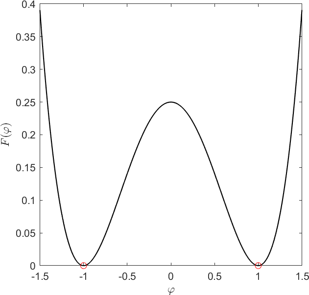
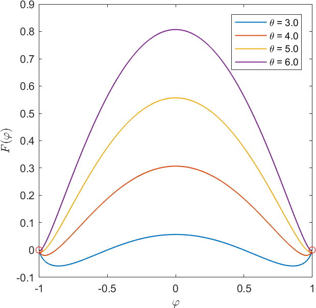
Figure 2.1: Ginzburg–Landau double-well potential(Left) and Flory–Huggins logarithmic potential(Right).

Indeed, the double-well potential penalizes sharp transition and helps to create the transition layer depicted in Fig. 1.1. The equilibrium configuration is the consequence of the competition between the two types of interactions. Let $\boldsymbol{u}$ be the velocity of incompressible fluids, the phase field $\varphi$ will evolve in time following a convective Cahn-Hilliard equation

$$\partial_{t}\varphi+{\rm div}(\varphi\boldsymbol{u})-{\rm div}\boldsymbol{J}_{\varphi}=0$$ (2.2)

where $\boldsymbol{J}_{\varphi}$ denotes the mass flux will be found later. Here we have used the incompressibility of fluids ${\rm div}\boldsymbol{u}=0$ to rewrite advection operator $(\boldsymbol{u}\cdot\nabla)\varphi$ in nonconservative form as the conservative form ${\rm div}(\varphi\boldsymbol{u})$.

The electromagnetic field adds to the total free energy a contribution essentially [51, 52],

$$E_{\boldsymbol{B},\boldsymbol{D}}=\frac{1}{2}\int_{\Omega}\frac{\boldsymbol{D}^{2}}{\varepsilon_{r}(\varphi)}+\frac{1}{2}\int_{\Omega}\frac{\boldsymbol{B}^{2}}{\mu_{r}(\varphi)},$$

where $\varepsilon_{r}(\varphi)$ is the dielectric constant,and $\boldsymbol{D}$ is the (electric) displacement vector, $\mu_{r}(\varphi)$ is the magnetic permeability and $\boldsymbol{B}$ is the magnetic displacement vector. However, since the displacement current and the inducted magnetic field are often neglected in the inductionless MHD [3, 6, 53], there is no contribution to the total energy from both the electric and magnetic field. With these simplifications, Maxwell equations are replaced by Poisson equation for the electric scalar potential,

$$\sigma(\varphi)^{-1}\boldsymbol{J}+\nabla\phi-\boldsymbol{u}\times\boldsymbol{B} =\boldsymbol{0},$$ (2.3)

$${\rm div}\boldsymbol{J} =0,$$

where $\boldsymbol{B}$ is the applied magnetic field which is assumed to be given. It is worth remarking that the first equation of (2.3) is obtained by combing generalized Ohm’s law with $\boldsymbol{E}=-\nabla\phi$, see [5, 53].

The inertia of the fluid would add a kinetic energy to the free energy of the form,

$$E_{\boldsymbol{u}}=\frac{1}{2}\int_{\Omega}\rho|\boldsymbol{u}|^{2},$$

where $\rho$ is the density of the fluid material. We model the incompressible flow by the following general evolution equations,

$$\rho\left(\partial_{t}\boldsymbol{u}+\boldsymbol{u}\cdot\nabla\boldsymbol{u}\right)-{\rm div}\mathbf{S}+\nabla p =\boldsymbol{F},$$ (2.4)

$${\rm div}\boldsymbol{u} =0.$$

where $p$ is the pressure, $\boldsymbol{F}$ is the field of forces exerted on the fluids, $\mathbf{S}$ denotes the symmetric stress tensor. In addition, we denote $\boldsymbol{\mathrm{T}}\coloneqq-p\boldsymbol{\mathrm{I}}+\mathbf{S}$ by stress. The expressions of $\boldsymbol{F}$ and $\mathbf{S}$ will be specified later. In this work, we consider two-phase inductionless magnetohydrodynamic fluids with matched density $\rho_{1}=\rho_{2}$. The extension to the non-matched density case will be discussed in Remark 1. Without lose of generality, we will set $\rho\equiv 1$ in the rest of this paper.

Thus, the total free energy is given as a sum of the interfacial energy $E_{\varphi}$ and the kinetic energy $E_{\boldsymbol{u}}$,

$$E=E_{\varphi}+E_{\boldsymbol{u}}.$$

We assume the velocity $\boldsymbol{u}$ and the fluxes $\boldsymbol{J}_{\phi}\cdot\boldsymbol{n}$, $\boldsymbol{J}\cdot\boldsymbol{n}$ to vanish at $\Sigma$, where $\boldsymbol{n}$ is the outer unit normal of $\Sigma$. The chemical potential $\mu$ is defined by the variational derivative of the energy $E$ with respect $\varphi$,

$$\mu\coloneqq\frac{\delta E}{\delta\varphi}=-\gamma\varepsilon\Delta\varphi+\frac{\gamma}{\varepsilon}f(\varphi).$$

With this notation, the time derivative of the free energy is given by

$$\frac{\mathrm{d}E}{\mathrm{d}t}=\int_{\Omega}\boldsymbol{u}\cdot\frac{\partial\boldsymbol{u}}{\partial t}+\int_{\Omega}\mu\frac{\partial\varphi}{\partial t}.$$

To deal with the divergence-free constraints for velocity and current density, we regard the pressure and electric potential as the corresponding Lagrange multipliers. Then we have

$$\frac{\mathrm{d}E}{\mathrm{d}t}=\int_{\Omega}\boldsymbol{u}\cdot\partial_{t}\boldsymbol{u}+\int_{\Omega}\mu\partial_{t}\varphi-\int_{\Omega}p\nabla\cdot\boldsymbol{u}-\int_{\Omega}\phi\nabla\cdot\boldsymbol{J}.$$ (2.5)

Next we rewrite some terms on the right hand side of (2.5). For the first and third terms, inserting the equation (2.4), integrating by parts and using the fact that the normal component of the velocity vanish at $\Sigma$ gives,

$$\int_{\Omega}\boldsymbol{u}\cdot\partial_{t}\boldsymbol{u}=-\int_{\Omega}\mathbf{S}:D\left(\boldsymbol{u}\right)+\int_{\Omega}\boldsymbol{u}\cdot\boldsymbol{F}.$$ (2.6)

where $D\left(\boldsymbol{u}\right)\coloneqq\frac{\nabla\boldsymbol{u}+\nabla\boldsymbol{u}^{{\rm T}}}{2}$ is strain velocity tensor. Analogously, inserting the equation (2.2), integrating by parts and using the fact that $\boldsymbol{J}_{\varphi}\cdot\boldsymbol{n}$ vanish at $\Sigma$ gives,

$$\int_{\Omega}\mu\partial_{t}\varphi=-\int_{\Omega}\boldsymbol{J}_{\varphi}\cdot\nabla\mu+\int_{\Omega}\varphi\nabla\mu\cdot\boldsymbol{u}.$$ (2.7)

For the last term, integrating by parts, inserting the equation (2.3) and using the fact that $\boldsymbol{J}\cdot\boldsymbol{n}$ vanish at $\Sigma$, we have

$$\int_{\Omega}\phi\nabla\cdot\boldsymbol{J}=-\int_{\Omega}\nabla\phi\cdot\boldsymbol{J}=\int_{\Omega}\sigma(\varphi)^{-1}\boldsymbol{J}\cdot\boldsymbol{J}-\int_{\Omega}\boldsymbol{u}\times\boldsymbol{B}\cdot\boldsymbol{J}.$$ (2.8)

Substituting (2.6)-(2.8) into (2.5), the time-derivative of the free energy can be rewritten as

$$\frac{\mathrm{d}E}{\mathrm{d}t}= -\int_{\Omega}\mathbf{S}:D(\boldsymbol{u})-\int_{\Omega}\boldsymbol{J}_{\varphi}\cdot\nabla\mu-\int_{\Omega}\sigma(\varphi)^{-1}\boldsymbol{J}\cdot\boldsymbol{J}$$ (2.9)

$$+\int_{\Omega}\boldsymbol{F}\cdot\boldsymbol{u}+\int_{\Omega}\varphi\nabla\mu\cdot\boldsymbol{u}-\int_{\Omega}\boldsymbol{J}\times\boldsymbol{B}\cdot\boldsymbol{u}.$$

Collecting all terms having a scalar product with the velocity in (2.9) gives the rate of change of the mechanical work with

$$\frac{\mathrm{d}W}{\mathrm{d}t}=\int_{\Omega}\boldsymbol{F}\cdot\boldsymbol{u}+\int_{\Omega}\varphi\nabla\mu\cdot\boldsymbol{u}-\int_{\Omega}\boldsymbol{J}\times\boldsymbol{B}\cdot\boldsymbol{u}.$$

Since no external forces are included into the system, we conclude that

$$\frac{\mathrm{d}W}{\mathrm{d}t}=0.$$

Therefore, we find an expression for the forces $\boldsymbol{F}$ acting on the fluid,

$$\boldsymbol{F}=-\varphi\nabla\mu+\boldsymbol{J}\times\boldsymbol{B}.$$

The first term $-\varphi\nabla\mu$ corresponds to surface tension, and the second term is the Lorentz force.

To determine the fluxes $\boldsymbol{J}_{\varphi}$ and the stress tensor $\mathbf{S}$, we turn to Onsager’s variational principle. We introduce the dissipation functional, which is the sum of quadratic in the fluxes with phenomenological parameters,

$$\Phi\left(\mathbf{J},\mathbf{J}\right)=\int_{\Omega}\frac{\left|\boldsymbol{J}_{\varphi}\right|^{2}}{2M(\varphi)}+\int_{\Omega}\frac{|\boldsymbol{J}|^{2}}{2\sigma(\varphi)}+\int_{\Omega}\frac{|\mathbf{S}|^{2}}{2\eta(\varphi)}$$ (2.10)

where the fluxes are $\mathbf{J}=\left(\mathbf{S},\boldsymbol{J}_{\varphi},\boldsymbol{J}\right)$. In (2.10), $M(\varphi)$ is the diffusional mobility related to the relaxation time scale, $\eta(\varphi)$ is the viscosity of the fluids and $\sigma(\varphi)$ is the electric conductivity. It means that the dissipation of $E$ stems from the friction losses, the Ohmic losses and the diffusion transport. The Onsager’s relation yields,

$$\delta_{\mathbf{J}}\left(\frac{\mathrm{d}E}{\mathrm{d}t}+\Phi\left(\mathbf{J},\mathbf{J}\right)\right)=0$$ (2.11)

Solving the variational problem (2.11), we obtain the fluxes

$$\boldsymbol{J}_{\varphi}=M(\varphi)\nabla\mu,\quad\mathbf{S}=2\eta(\varphi)D\left(\boldsymbol{u}\right).$$

These “constitutive” relations can be also obtained by assuming that the fluxes depend linearly on the thermodynamic forces. In fact, it is implicitly postulated in the form of the dissipation function $\Phi$.

To summarize, we obtain the incompressible Cahn–Hilliard–Inductionless-MHD system,

$$\boldsymbol{u}_{t}+\boldsymbol{u}\cdot\nabla\boldsymbol{u}-2\nabla\left(\eta\left(\varphi\right)D\left(\boldsymbol{u}\right)\right)+\nabla p-\boldsymbol{J}\times\boldsymbol{B}+\varphi\nabla\mu =\boldsymbol{0},$$ (2.12)

$$\mathrm{div}\boldsymbol{u} =0,$$ (2.13)

$$\sigma\left(\varphi\right)^{-1}\boldsymbol{J}+\nabla\phi-\boldsymbol{u}\times\boldsymbol{B} =\boldsymbol{0},$$ (2.14)

$$\mathrm{div}\boldsymbol{J} =0,$$ (2.15)

$$\varphi_{t}+{\rm div}(\varphi\boldsymbol{u})-{\rm div}\left(M\left(\varphi\right)\nabla\mu\right) =0,$$ (2.16)

$$-\gamma\varepsilon\Delta\varphi+\frac{\gamma}{\varepsilon}f(\varphi)-\mu =0,$$ (2.17)

with the following initial and boundary conditions

$$\boldsymbol{u}(0)=\boldsymbol{u}^{0},\quad\varphi(0) =\varphi^{0},$$ (2.18)

$$\boldsymbol{u}=0,\quad\boldsymbol{J}\cdot\boldsymbol{n} =0,$$ (2.19)

$$\partial_{\boldsymbol{n}}\varphi=0,\quad M\left(\varphi\right)\partial_{\boldsymbol{n}}\mu =0.$$ (2.20)

The dynamic behavior of the flow is governed by the coupling model of the Cahn-Hilliard equations, the Navier-Stokes equations and the Poisson equation. As mentioned earlier, the last term on the left-hand side of (2.12) the continuum surface tension force in the potential form. This term appears differently in different literature [23, 24, 37]: $-\nabla\cdot(\nabla\varphi\otimes\nabla\varphi),$ $-\mu\nabla\varphi,$ or $\varphi\nabla\mu.$ It can be shown that the three expressions are equivalent by redefining the pressure $p$. To deal with the discontinuous of material properties, we assume that all the material properties $\Psi\in\left\{\eta\left(\varphi\right),\sigma\left(\varphi\right)^{-1}\right\}$ that depend on the phase is a Lipschitz-continuous function of $\varphi$ satisfying

$$0<\min\left\{\Psi_{1},\Psi_{2}\right\}\leq\Psi(\phi)\leq\max\left\{\Psi_{1},\Psi_{2}\right\}.$$

where $\Psi_{i}$ is the material parameter of the fluid $i$.

Remark 1.

Though the model considered is for match-density two-phase system, one can still employ this with Boussinesq approximation in the case of small density ratio [23]. Specifically, a gravitational force are supplemented to the right hand side of the momentum equations (2.12) to model the effect of density difference. The modeling and analysis for large density ratio case are ongoing.

Remark 2.

The model that we derived can be generalized to handle situations that requires other physical factors easily. As a representative example, we present the sketch of an extension for the model (2.1) with moving contact lines in A. To more general situation when either the system is subjected to gravitational forces or when one additional soluble species is present in both fluids, we refer to [26, 54].

To end this section, we present the energy law for the CHiMHD system.

Theorem 3.

Let $(\boldsymbol{u},p,\boldsymbol{J},\phi,\varphi,\mu)$ be the solution of (2.2). The energy law holds

$$\frac{\mathrm{d}E}{\mathrm{d}t}=-\Phi.$$ (2.21)

where

$$E =\int_{\Omega}\left(\frac{1}{2}|\boldsymbol{u}|^{2}+\frac{\lambda\epsilon}{2}|\nabla\varphi|^{2}+\frac{\lambda}{\epsilon}F(\varphi)\right),$$

$$\Phi =\int_{\Omega}\left(2\eta(\varphi)\left|D(\boldsymbol{u})\right|^{2}+M(\varphi)\left|\nabla\mu\right|^{2}+\sigma(\varphi)^{-1}|\boldsymbol{J}|^{2}\right).$$

Proof.

An immediate consequence of (2.9) gives the theorem. ∎

The energy law describes the variation of the total energy caused by energy conversion, which is crucial to the analysis of and the design of unconditionally stable numerical schemes for the model.

3 Sharp Interface Asymptotic

In this section, we perform formally matched asymptotic expansions to derive the sharp-interface limits of a phase-field model. The idea of the method is to plug the outer and inner expansions into the model equations and solve them order by order, in addition these expansions should match up [55, 56, 57]. To make the presentation clear, we adopt $\omega_{\varepsilon}\in\left\{\boldsymbol{u}_{\varepsilon},p_{\varepsilon},\boldsymbol{J}_{\epsilon},\phi_{\epsilon},\varphi_{\varepsilon},\mu_{\varepsilon}\right\}$ instead of $\omega\in\left\{\boldsymbol{u},p,\boldsymbol{J},\phi,\varphi,\mu\right\}$ in the system (2.1) to stress that these functions depend on $\varepsilon$. We use the notation $(\cdot)_{o}^{a}$ and $(\cdot)_{I}^{a}$ for the terms resulting from the order $a$ outer and inner expansions of (2.1), respectively.

For any $\epsilon>0$ and for each time $t\in[0,T],$given a function $\varphi_{\epsilon}\left(x,t\right)$, we define its zero-level sets as

$$\Gamma_{\epsilon}:=\left\{(x,t)\in\Omega\times[0,T]:\varphi_{\epsilon}(x,t)=0\right\}.$$

Two open subdomains are separated by $\Gamma_{\epsilon}$ are denoted by

$$\Omega_{+}(\epsilon,t):=\left\{x\in\Omega:\varphi_{\epsilon}(x,t)>0\right\},\quad\Omega_{-}(\epsilon,t):=\left\{x\in\Omega:\varphi_{\epsilon}(x,t)<0\right\}.$$

We consider the model (2.1) with the following choices and assumptions [36, 44, 58].

1. We assume that $\Gamma_{\epsilon}\subseteq\Omega$ are closed evolving hyper-surface, which depend smoothly on $t$ and $\epsilon$ and converge as $\epsilon\rightarrow 0$ to a limiting evolving hyper-surface $\Gamma$ which moving with normal velocity $\mathcal{V}$. Further, for every $\epsilon>0$, we assume that the domain $\Omega$ can be divided into two subdomains $\Omega_{+}(\epsilon,t)$ and $\Omega_{-}(\epsilon,t)$, and $\Omega_{+}(\epsilon,t)$ is the region enclosed by $\Gamma_{\epsilon}$.

2. The solutions to (2.1) $\left(\boldsymbol{u}_{\varepsilon},p_{\varepsilon},\boldsymbol{J}_{\epsilon},\phi_{\epsilon},\varphi_{\varepsilon},\mu_{\varepsilon}\right)_{\epsilon>0}$ are assumed to be sufficiently smooth so that they have an asymptotic expansion with respect to $\epsilon$ in the bulk regions away from $\Gamma$ (outer expansion), and another expansion in the interfacial region close to $\Gamma$ (inner expansion).

3. For the mobility $m_{\varepsilon}$, we distinguish three cases:

   $$M_{\varepsilon}(\varphi)=\left\{\begin{array}[]{ll}m_{0}&\text{ case I },\\ \varepsilon m_{0}&\text{ case II },\\ m_{0}\left(1-\varphi^{2}\right)_{+}&\text{ case III },\end{array}\right.$$ (3.1)

   where $m_{0}$ is a positive constant, $(\cdot)_{+}$ is defined by

   $$(a)_{+}=\begin{cases}a&a\geq 0,\\ 0&a<0.\end{cases}$$

To make the presentation in this section clear, we only present the sharp interface asymptotic analysis for the Ginzburg-Landau double-well potential $F(\varphi)=\frac{1}{4}\left(\varphi^{2}-1\right)^{2}$. The extension to general potentials is trivial. We omit the details but give a sketch in Remark 5.

3.1 Outer expansion

We first expand the solution in outer regions away from the interface. For $\omega_{\varepsilon}\in\left\{\boldsymbol{u}_{\varepsilon},p_{\varepsilon},\boldsymbol{J}_{\epsilon},\phi_{\epsilon},\varphi_{\varepsilon},\mu_{\varepsilon}\right\},$ the assumption 2 implies the following outer expansions,

$$\omega_{\varepsilon}=\omega_{0}+\varepsilon\omega_{1}+\varepsilon^{2}\omega_{2}+\cdots.$$

We substitute the above expansions to the CHiMHD system. The leading order, $\text{\eqref{model:ch}}_{O}^{-1}$ gives

$$f\left(\varphi_{0}\right)=0$$ (3.2)

The stable solutions of (3.2) corresponding to the minima of $F$ are $\varphi_{0}=\pm 1.$ Thus, we can define the domain occupied of fluid 1 and fluid 2 by

$$\Omega_{-}:=\left\{x\in\Omega:\varphi_{0}(x)=-1\right\},\quad\Omega_{+}:=\left\{x\in\Omega:\varphi_{0}(x)=1\right\}.$$

A sketch of the situation is shown in Fig. 3.1.

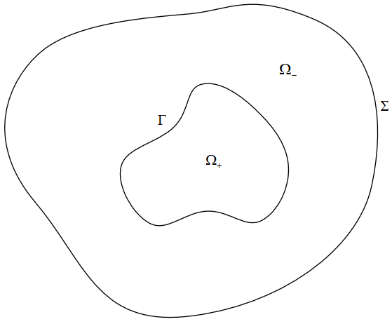
Figure 3.1: The domain occupied of fluid 1 and fluid 2.

For the equations (2.13) and (2.15), in the leading order, $\text{\eqref{model:divu}}_{O}^{-1}$ and $\text{\eqref{model:divJ}}_{O}^{-1}$, we have

$$\nabla\cdot\boldsymbol{u}_{0}=0,\quad\nabla\cdot\boldsymbol{J}_{0}=0.$$

Since $\nabla\varphi_{0}=\boldsymbol{0}$ in $\Omega_{+}\cup\Omega_{-}$ , we obtain for the equations in $\Omega_{+}\cup\Omega_{-}$ to zeroth order that

$$\partial_{t}\boldsymbol{u}_{0}+\left(\boldsymbol{u}_{0}\cdot\nabla\right)\boldsymbol{u}_{0}-2\eta_{i}{\rm div}\left(D\left(\boldsymbol{u}_{0}\right)\right)+\nabla p_{0}-\boldsymbol{J}_{0}\times\boldsymbol{B} =\boldsymbol{0},$$ (3.3)

$${\rm div}\boldsymbol{u}_{0} =0,$$

$$\sigma_{i}^{-1}\boldsymbol{J}_{0}+\nabla\varphi_{0}-\boldsymbol{u}_{0}\times\boldsymbol{B} =\boldsymbol{0},$$

$$\mathrm{div}\boldsymbol{J}_{0} =0.$$

Note that this is the standard inductionless MHD equations in each subdomain.

We now analyze (2.17) according to the mobilities introduced in (3.1). For the cases of $M(\varphi)=\epsilon m_{0}$ and $M(\varphi)=m_{0}\left(1-\varphi^{2}\right)_{+}$, the chemical potential does not contribute to the equations at zeroth order. In this case of $M(\varphi)=m_{0}$, we obtain a Poisson equation for $\mu_{0}$,

$$\Delta\mu_{0}=0.$$

3.2 Inner Expansion

We now do an expansion in an interfacial region. This subsection uses ideas presented in [26, 36, 59, 60].

3.2.1 New Coordinates and matching conditions

We first introduce new coordinates in a neighborhood of $\Gamma$. To this end, we consider the signed distance function $d(x,t)$ of a point $x$ to $\Gamma$ with $d(x,t)>0$ if $x\in\Omega_{+}$ and $d(x,t)<0$ if $x\in\Omega_{-}.$ Note that it is well-defined near the interface and $\mathcal{V}=-\partial_{t}d$. By $\boldsymbol{\nu}=\nabla d$ we denote the unit normal to $\Gamma$ pointing into the region $\Omega_{+}$. Introduce a new re-scaled variable

$$\xi=\frac{d(x,t)}{\varepsilon}.$$

In a tubular neighborhood of $\Gamma$, for any function $\omega(x,t)$, we can rewrite it as

$$\omega(x,t)=\tilde{\omega}(x,\xi,t).$$

In this new $(t,x,\xi)$-coordinate system, the following change of variables apply,

$$\begin{array}[]{l}\nabla\omega=\nabla\tilde{\omega}+\varepsilon^{-1}\partial_{\xi}\tilde{\omega}\boldsymbol{\nu},\\ \Delta\omega=\Delta\tilde{\omega}-\varepsilon^{-1}\partial_{\xi}\tilde{\omega}\kappa+2\varepsilon^{-1}(\boldsymbol{\nu}\cdot\nabla)\partial_{\xi}\tilde{\omega}+\varepsilon^{-2}\partial_{\xi\xi}\tilde{\omega},\\ \partial_{t}\omega=\partial_{t}\tilde{\omega}+\varepsilon^{-1}\partial_{\xi}\tilde{\omega}\partial_{t}d,\end{array}$$

where $\kappa=-\nabla\cdot\boldsymbol{\nu}$ is the mean curvature of the interface. In particular, if $\boldsymbol{\omega}$ is a vector-valued function for $x$ in a tubular neighborhood of $\Sigma_{0},$ then we obtain

$${\rm div}\boldsymbol{\omega} ={\rm div}\tilde{\boldsymbol{\omega}}+\varepsilon^{-1}\partial_{\xi}\tilde{\boldsymbol{\omega}}\cdot\boldsymbol{\nu},$$

$$\nabla\boldsymbol{\omega} =\nabla\tilde{\boldsymbol{\omega}}+\varepsilon^{-1}\partial_{\xi}\tilde{\boldsymbol{\omega}}\otimes\boldsymbol{\nu},$$

$$D\left(\boldsymbol{\omega}\right) =\mathcal{E}\left(\nabla\tilde{\boldsymbol{\omega}}\right)+\varepsilon^{-1}\mathcal{E}\left(\partial_{\xi}\tilde{\boldsymbol{\omega}}\otimes\boldsymbol{\nu}\right),$$

where $\mathcal{E}\left(\boldsymbol{A}\right)\coloneqq\left(\boldsymbol{A}+\boldsymbol{A}^{{\rm T}}\right)/2$.

We denote the variables $\omega_{\epsilon}\in\left\{\boldsymbol{u}_{\varepsilon},p_{\varepsilon},\boldsymbol{J}_{\epsilon},\phi_{\epsilon},\varphi_{\varepsilon},\mu_{\varepsilon}\right\}$ in the new coordinate system by $\tilde{\omega}_{\varepsilon}\in\left\{\tilde{\boldsymbol{u}}_{\varepsilon},\tilde{p}_{\varepsilon},\tilde{\boldsymbol{J}}_{\epsilon},\tilde{\phi}_{\epsilon},\tilde{\varphi}_{\varepsilon},\tilde{\mu}_{\varepsilon}\right\}$. The assumption means that they have the following inner expansions,

$$\tilde{\omega}_{\varepsilon}=\tilde{\omega}_{0}+\varepsilon\tilde{\omega}_{1}+\varepsilon^{2}\tilde{\omega}_{2}+\cdots.$$

The assumption that the zero level sets of $\varphi_{\varepsilon}$ converge to $\Gamma$ implies that

$$\tilde{\varphi}_{0}(x,0,t)=0.$$ (3.4)

In matched asymptotic techniques, inner and outer quantities are linked together by matching conditions. For this end, we employ the matching conditions [36, 44, 58]:

$$\underset{\xi\rightarrow\pm\infty}{\lim}\tilde{\omega}_{0}(x,\xi,t) =\omega_{0}^{\pm}(x),$$ (3.5)

$$\underset{\xi\rightarrow\pm\infty}{\lim}\partial_{\xi}\tilde{\omega}_{0}(x,\xi,t) =0,$$ (3.6)

$$\underset{\xi\rightarrow\pm\infty}{\lim}\left(\partial_{\xi}\tilde{\omega}_{1}(x,\xi,t)+\nabla\tilde{\omega}_{0}\right) =\nabla\omega_{0}^{\pm}(x)\cdot\boldsymbol{\nu}.$$ (3.7)

where $\omega^{\pm}$ denotes the restriction of a function $\omega$ in $\Omega_{+}$ and $\Omega_{-}$ respectively. Moreover, we denote the jump of a quantity $\omega$ across the interface by

$$\left[\omega\right]:=\omega^{+}(x,t)-\omega^{-}(x,t).$$

3.2.2 The equations to leading order

We begin with considering the equation (2.17). The leading order $\eqref{model:chc}_{I}^{-1}$ yields

$$\partial_{\xi\xi}\tilde{\varphi}_{0}-f\left(\tilde{\varphi}_{0}\right)=0$$ (3.8)

Invoking with (3.4) we obtain that $\tilde{\varphi}_{0}$ is independent of $x$ and $t$. Thus, we write $\tilde{\varphi}_{0}^{\prime}(\xi)$ and $\tilde{\varphi}_{0}^{\prime\prime}(\xi)$ instead of $\partial_{\xi}\tilde{\varphi}_{0}$ and $\partial_{\xi\xi}\tilde{\varphi}_{0}$. As a consequence, $\tilde{\varphi}_{0}$ is only a function of $\xi$, and fulfills

$$\tilde{\varphi}_{0}^{\prime\prime}(\xi)-f\left(\tilde{\varphi}_{0}(\xi)\right)=0,\quad\tilde{\varphi}_{0}(0)=0,\quad\underset{\xi\rightarrow\pm\infty}{\lim}\tilde{\varphi}_{0}(\xi)=\pm 1,$$ (3.9)

where we have employed the match condition (3.5). For the Ginzburg–Landau double-well potential, the unique solution is given by

$$\tilde{\varphi}_{0}(\xi)=\tanh\left(\xi/\sqrt{2}\right).$$

Multiplying (3.9) by $\tilde{\varphi}_{0}^{\prime}(\xi)$, integrating and applying the matching conditions (3.5) and (3.6) to $\tilde{\varphi}_{0}(\xi)$, we obtain the equipartition of energy [61]

$$\frac{1}{2}\left|\tilde{\varphi}_{0}^{\prime}(\xi)\right|^{2}=F\left(\tilde{\varphi}_{0}(\xi)\right)\text{ for all }|\xi|<\infty.$$

Consequently, we have

$$\iota\coloneqq\int_{-\infty}^{\infty}\left|\partial_{\xi}\tilde{\phi}_{0}^{\prime}\right|^{2}\mathrm{d}\xi =\int_{-\infty}^{\infty}\left|\partial_{\xi}\tilde{\phi}_{0}^{\prime}\right|\sqrt{2F\left(\tilde{\phi}_{0}\right)}\mathrm{d}\xi=\frac{2\sqrt{2}}{3}.$$

Next, equations (2.13) and (2.15) yields the leading order $\text{\eqref{model:divu}}{}_{I}^{-1}$ and $\text{\eqref{model:divJ}}{}_{I}^{-1}$,

$$\boldsymbol{\nu}\cdot\partial_{\xi}\tilde{\boldsymbol{u}}_{0}=0,\quad\boldsymbol{\nu}\cdot\partial_{\xi}\tilde{\boldsymbol{J}}_{0}=0.$$ (3.10)

Upon integrating the equation with respect to $\xi$ in $(-\infty,\infty)$, using $\partial_{\xi}\boldsymbol{\nu}=0$ and the matching condition (3.5), we obtain

$$\left[\boldsymbol{u}_{0}\cdot\boldsymbol{\nu}\right]=0,\quad\left[\boldsymbol{J}_{0}\cdot\boldsymbol{\nu}\right]=0.$$

Then, we turn to the he momentum equation (2.12). From the leading order $\eqref{model:fluid}_{I}^{-2}$, we get

$$\varepsilon^{-2}\partial_{\xi}\left(\eta\left(\tilde{\varphi}_{0}\right)\mathcal{E}\left(\partial_{\xi}\tilde{\boldsymbol{u}}_{0}\otimes\boldsymbol{\nu}\right)\boldsymbol{\nu}\right)=0.$$

Invoking with (3.10), we have

$$2\mathcal{E}\left(\partial_{\xi}\tilde{\boldsymbol{u}}_{0}\otimes\boldsymbol{\nu}\right)\boldsymbol{\nu}=\partial_{\xi}\tilde{\boldsymbol{u}}_{0}.$$

Thus, we conclude that

$$\partial_{\xi}\left(\eta\left(\tilde{\varphi}_{0}(\xi)\right)\left(\partial_{\xi}\tilde{\boldsymbol{u}}_{0}\right)\right)=0.$$

Integrating from $-\infty$ to $\xi$ with $|\xi|<\infty,$ using the matching condition (3.6) and the positivity of $\eta(\cdot),$ it gives

$$\partial_{\xi}\tilde{\boldsymbol{u}}_{0}=\mathbf{0}.$$

Once more integrating with respect to $\xi$ in $(-\infty,\infty)$ and using the matching condition (3.5) yields

$$\left[\boldsymbol{u}_{0}\right]=\mathbf{0}.$$

Now we analyze the equation (2.14) at leading order $\eqref{model:poisson}{}_{I}^{-1}$,

$$\boldsymbol{\nu}\partial_{\xi}\tilde{\phi}_{\epsilon}=\boldsymbol{0}.$$

Integrating and applying the matching condition (3.5) to $\tilde{\phi}_{\epsilon}$ leads to

$$\left[\phi_{0}\right]=0.$$

Finally, we consider (2.16). We distinguish again the two cases for the mobilities:

• Case I : At order $\epsilon^{-2}$, we obtain from $\eqref{model:ch}{}_{I}^{-2}$ ,

  $$\partial_{\xi\xi}\tilde{\mu}_{0}=0.$$

• Case II : We obtain from $\eqref{model:ch}{}_{I}^{-1}$ that

  $$\partial_{t}d\partial_{\xi}\tilde{\varphi}_{0}+\partial_{\xi}\left(\tilde{\varphi}_{0}\tilde{\boldsymbol{u}}_{0}\right)\cdot\boldsymbol{\nu}=m_{0}\partial_{\xi\xi}\tilde{\mu}_{0}$$

  Integrating this identity with respect to $\xi$ and using the matching condition (3.6) give

  $$\partial_{t}d+\boldsymbol{u}_{0}\cdot\boldsymbol{\nu}=0$$

  This implies that the normal velocity of the interface $\Gamma$ is given by

  $$\mathcal{V}=\boldsymbol{u}_{0}\cdot\boldsymbol{\nu}$$

  In particular, we obtain that

  $$\partial_{\xi\xi}\tilde{\mu}_{0}=0.$$

Thus, for the Case I and Case II, similar to the arguments for $\tilde{\boldsymbol{u}}_{0}$, we obtain $\mu_{0}$ is independent of $\xi$, and

$$\left[\mu_{0}\right]=0.$$

• Case III : From $\eqref{model:ch}{}_{I}^{-2}$, we get

  $$\partial_{t}d\partial_{\xi}\tilde{\varphi}_{0}+\partial_{\xi}\left(\tilde{\varphi}_{0}\tilde{\boldsymbol{u}}_{0}\right)\cdot\boldsymbol{\nu}=\partial_{\xi}\left(m_{0}\left(1-\tilde{\varphi}_{0}^{2}\right)\partial_{\xi}\tilde{\mu}_{0}\right).$$

  The similar arguments as above yields

  $$\mathcal{V}=\boldsymbol{u}_{0}\cdot\boldsymbol{\nu}$$

  and

  $$\partial_{\xi}\left(m_{0}\left(1-\tilde{\varphi}_{0}^{2}\right)\partial_{\xi}\tilde{\mu}_{0}\right) =0.$$

  Integrating it from $-\infty$ to $\xi$ with $|\xi|<\infty$ and using the matching condition (3.6) yields

  $$m_{0}\left(1-\tilde{\varphi}_{0}^{2}\right)\partial_{\xi}\tilde{\mu}_{0}=0.$$

  Note that $\left|\tilde{\varphi}_{0}\right|<1$ for $|\xi|<\infty$, this implies that

  $$\partial_{\xi}\tilde{\mu}_{0}=0.$$

  Thus, we conclude that $\mu_{0}$ is independent of $\xi$, and

  $$\left[\mu_{0}\right]=0.$$

3.2.3 Inner Expansion to higher order

We will now expand the equations in the inner regions to the next highest order for obtaining contributions of the diffusive fluxes in the interface, and the momentum balance in the sharp interface limit.

First of all, from $\text{\eqref{model:chc}}{}_{I}^{0}$, we obtain

$$\tilde{\mu}_{0}=\lambda f^{\prime}\left(\tilde{\varphi}_{0}\right)\tilde{\varphi}_{1}-\lambda\partial_{\xi\xi}\tilde{\varphi}_{1}+\lambda\partial_{\xi}\tilde{\varphi}_{0}\kappa$$

Multiplying by $\partial_{\xi}\tilde{\phi}_{0}$ and integrating from $-\infty$ to $+\infty$, and applying the fact $\tilde{\mu}_{0}$ is independent of $\xi$ and the matching condition (3.5) yields

$$2\mu_{0} =\int_{-\infty}^{\infty}\tilde{\mu}_{0}\partial_{\xi}\tilde{\varphi}_{0}\mathrm{d}\xi=\int_{-\infty}^{\infty}\lambda\partial_{\xi}\left(f\left(\tilde{\varphi}_{0}\right)\right)\tilde{\varphi}_{1}-\lambda\partial_{\xi\xi}\tilde{\varphi}_{1}\partial_{\xi}\tilde{\varphi}_{0}+\lambda\kappa\left|\partial_{\xi}\tilde{\varphi}_{0}\right|^{2}\mathrm{d}\xi$$

$$=\int_{-\infty}^{\infty}\lambda\partial_{\xi}\left(f\left(\tilde{\varphi}_{0}\right)\right)\tilde{\varphi}_{1}-\lambda\partial_{\xi\xi}\tilde{\varphi}_{1}\partial_{\xi}\tilde{\varphi}_{0}+\lambda\kappa\iota$$

Using the matching conditions (3.5) and (3.6), (3.8) and $f(\pm 1)=0,$ integration by parts gives

$$\int_{-\infty}^{\infty}\partial_{\xi}\left(f\left(\tilde{\varphi}_{0}\right)\right)\tilde{\varphi}_{1}-\partial_{\xi\xi}\tilde{\varphi}_{1}\partial_{\xi}\tilde{\varphi}_{0}\mathrm{d}\xi= \left[f\left(\tilde{\varphi}_{0}\right)\tilde{\varphi}_{1}-\partial_{\xi}\tilde{\varphi}_{1}\partial_{\xi}\tilde{\varphi}_{0}\right]_{-\infty}^{+\infty}$$

$$-\int_{-\infty}^{\infty}\partial_{\xi}\tilde{\varphi}_{1}\left(f\left(\tilde{\varphi}_{0}\right)-\partial_{\xi\xi}\tilde{\varphi}_{0}\right)\mathrm{d}\xi=0$$

Introducing the scaled surface tension between the two phases $\hat{\lambda}=\lambda\iota$, Collecting these equalities gives

$$2\mu_{0}=\hat{\lambda}\kappa$$ (3.11)

This is a solvability condition for $\tilde{\varphi}_{1}$, the so-called Gibbs-Thomas equation [26, 44].

Now we analyze (2.16) only for the mobilities (3.1) for the Case I. For the Case II and Case III, the mobility does not contribute to the sharp interface limit. Using $\partial_{\xi}\tilde{\mu}_{0}=0$ and from $\text{\eqref{model:ch}}_{I}^{-1}$, we obtain

$$\left(-\mathcal{V}+\tilde{\boldsymbol{u}}_{0}\cdot\boldsymbol{\nu}\right)\partial_{\xi}\tilde{\varphi}_{0}=m_{0}\partial_{\xi\xi}\tilde{\mu}_{1}$$

Integrating with respect to $\xi$ from $-\infty$ to $\infty,$ using the matching condition (3.7) yields

$$2\left(-\mathcal{V}+\boldsymbol{u}_{0}\cdot\boldsymbol{\nu}\right)=m_{0}\left[\nabla\mu_{0}\cdot\boldsymbol{\nu}\right]$$

Finally, we analyze (2.12). We obtain the equation (2.12) at order $\epsilon^{-1}$, $\text{\eqref{model:fluid}}{}_{I}^{-1}$ ,

$$\partial_{\xi}\left(2\eta\left(\tilde{\varphi}_{0}\right)\mathcal{E}\left(\partial_{\xi}\tilde{\boldsymbol{u}}_{1}\otimes\boldsymbol{\nu}\right)\boldsymbol{\nu}\right)+\partial_{\xi}\left(2\eta\left(\tilde{\varphi}_{0}\right)\mathcal{E}\left(\nabla\tilde{\boldsymbol{u}}_{0}\right)\boldsymbol{\nu}\right)-\partial_{\xi}\tilde{p}_{0}\boldsymbol{\nu}+\mu_{0}\partial_{\xi}\tilde{\varphi}_{0}\boldsymbol{\nu}=0.$$ (3.12)

Using the match condition (3.7) to $\tilde{\boldsymbol{u}}_{1}$, we have

$$\underset{\xi\rightarrow\pm\infty}{\lim}\left(\partial_{\xi}\tilde{\boldsymbol{u}}_{1}\otimes\boldsymbol{\nu}+\nabla\tilde{\boldsymbol{u}}_{0}\right)=\nabla\boldsymbol{u}_{0}.$$

Integrating (3.12) with respect to $\xi$, using (3.11) and after matching gives

$$\left[2\eta D(\boldsymbol{u}_{0})\boldsymbol{\nu}-p\boldsymbol{\nu}\right]=\hat{\lambda}\kappa\boldsymbol{\nu}.$$

It should be noted that this is the classical jump condition for the stress [37].

3.3 Sharp interface limits and energy inequalities

First of all, we summarize the sharp interface limits for (2.1) with the different mobilities. In the sharp interface limits, not only do we need to seek for the functions $\left(\boldsymbol{u},p,\boldsymbol{J},\phi,\mu\right)$ for Case I or $\left(\boldsymbol{u},p,\boldsymbol{J},\phi\right)$ for Cases II and III, but we also need to look for a smoothly evolving hyper-surface $\Gamma$. Specifically,

• Case I : The six-tuple $\left(\Gamma,\boldsymbol{u},p,\boldsymbol{J},\phi,\mu\right)$ satisfies

$$\partial_{t}\boldsymbol{u}+\left(\boldsymbol{u}\cdot\nabla\right)\boldsymbol{u}-2\eta_{i}{\rm div}\left(D\left(\boldsymbol{u}\right)\right)+\nabla p-\boldsymbol{J}\times\boldsymbol{B} =\boldsymbol{0}\quad\text{in }\Omega\times(0,\mathrm{T}],$$ (3.13)

$${\rm div}\boldsymbol{u} =0\quad\text{in }\Omega\times(0,\mathrm{T}],$$

$$\sigma_{i}^{-1}\boldsymbol{J}+\nabla\phi-\boldsymbol{u}\times\boldsymbol{B} =\boldsymbol{0}\quad\text{in }\Omega\times(0,\mathrm{T}],$$

$$\mathrm{div}\boldsymbol{J} =0\quad\text{in }\Omega\times(0,\mathrm{T}],$$

$$\Delta\mu =0\quad\text{in }\Omega\times(0,\mathrm{T}],$$

$$\left[2\eta D(\boldsymbol{u})\boldsymbol{\nu}-p\boldsymbol{\nu}\right]=\hat{\lambda}\kappa\boldsymbol{\nu},\quad\left[\boldsymbol{u}\right] =0\quad\text{on }\Gamma\times(0,\mathrm{T}],$$

$$\left[\boldsymbol{J}\cdot\boldsymbol{\nu}\right]=0,\quad\left[\phi\right] =0\quad\text{on }\Gamma\times(0,\mathrm{T}],$$

$$2\left(-\mathcal{V}+\boldsymbol{u}\cdot\boldsymbol{\nu}\right)=m_{0}\left[\nabla\mu\right]\cdot\boldsymbol{\nu},\quad 2\mu =\hat{\lambda}\kappa\quad\text{on }\Gamma\times(0,\mathrm{T}],$$

together with the boundary and initial conditions

$$\boldsymbol{u}(0) =\boldsymbol{u}^{0}\quad\text{ in }\Omega,$$ (3.14)

$$\boldsymbol{u}=0,\quad\boldsymbol{J}\cdot\boldsymbol{n}=0,\quad\partial_{\boldsymbol{n}}\mu =0\text{ on }\Sigma\times(0,\mathrm{T}],$$ (3.15)

$$\Gamma\left(0\right) =\Gamma_{0}$$ (3.16)

• Case II and III : The five-tuple $\left(\Gamma,\boldsymbol{u},p,\boldsymbol{J},\phi\right)$ satisfies

$$\partial_{t}\boldsymbol{u}+\left(\boldsymbol{u}\cdot\nabla\right)\boldsymbol{u}-2\eta_{i}{\rm div}\left(D\left(\boldsymbol{u}\right)\right)+\nabla p-\boldsymbol{J}\times\boldsymbol{B} =\boldsymbol{0}\quad\text{in }\Omega\times(0,\mathrm{T}],$$ (3.17)

$${\rm div}\boldsymbol{u} =0\quad\text{in }\Omega\times(0,\mathrm{T}],$$

$$\sigma_{i}^{-1}\boldsymbol{J}+\nabla\phi-\boldsymbol{u}\times\boldsymbol{B} =\boldsymbol{0}\quad\text{in }\Omega\times(0,\mathrm{T}],$$

$$\mathrm{div}\boldsymbol{J} =0\quad\text{in }\Omega\times(0,\mathrm{T}],$$

$$\left[2\eta D(\boldsymbol{u})\boldsymbol{\nu}-p\boldsymbol{\nu}\right]=\hat{\lambda}\kappa\boldsymbol{\nu},\quad\left[\boldsymbol{u}\right] =0\quad\text{on }\Gamma\times(0,\mathrm{T}],$$

$$\left[\boldsymbol{J}\cdot\boldsymbol{\nu}\right]=0,\quad\left[\phi\right] =0\quad\text{on }\Gamma\times(0,\mathrm{T}],$$

$$\mathcal{V} =\boldsymbol{u}\cdot\boldsymbol{\nu}\quad\text{on }\Gamma\times(0,\mathrm{T}],$$

together with the boundary and initial conditions

$$\boldsymbol{u}(0) =\boldsymbol{u}^{0}\quad\text{ in }\Omega,$$ (3.18)

$$\boldsymbol{u}=0,\quad\boldsymbol{J}\cdot\boldsymbol{n} =0\text{ on }\Sigma\times(0,\mathrm{T}],$$ (3.19)

$$\Gamma\left(0\right) =\Gamma_{0}$$ (3.20)

It is remarkable that Case I has distinctive features on the bulk equations and interface conditions, compared with Case II and III.

• Bulk equations: For the case of $M\left(\varphi\right)=\epsilon m_{0}$ tends to zero or $M\left(\varphi\right)=m_{0}\left(1-\varphi\right)_{+}^{2}$ degenerates in the bulk, the equations are standard inductionless MHD equations. While in the case of a constant mobility $M\left(\varphi\right)=m_{0}$, a harmonic equation for the chemical potential are incorporated in addition due to the diffusion of mass.

• Interface conditions: The three cases under consideration gives the same interface conditions for hydrodynamics and electrostatics, the velocity is continuous and the stress tensor fulfills the Yong-Laplace law, the current density is normal-continuous and the electric potential is continuous. For Case I, the interface condition for the chemical potential is an identity, which indicate that $\mu$ is a constant related the surface tension coefficient and the mean curvature of the interface. A crucial observation is that the evolution of the interface is quite different. In Case II and III, we get the usual kinematic condition that the interface is only transported by the flow of the surrounding fluids. Roughly speaking, the fluid interface evolves as a scaled mean curvature flow [38]. However, in Case I, the interface is no longer material and the interface condition is of Stefan type condition. Both the velocity of the fluid and the jump of the flux of the chemical potential on the interface contribute the normal velocity of the interface.

Finally, we derive a formal energy law fo the sharp interface model.

Theorem 4.

Assume the solution to the sharp interface problems and the evolving hyper-surface $\Gamma\subset\Omega$ are sufficiently smooth, then it holds

$$\frac{{\rm d}}{{\rm d}t}\left[\int_{\Omega}\left(\frac{1}{2}|\boldsymbol{u}|^{2}\right)+\int_{\Gamma}\hat{\lambda}\right]=-\mathcal{D}\leq 0$$ (3.21)

where the dissipation quantity $\mathcal{D}$ is defined by

$$\textrm{\text{ {Case I} }}: \mathcal{D}=\int_{\Omega}2\eta\left|D\left(\boldsymbol{u}\right)\right|^{2}+\int_{\Omega}\sigma^{-1}\left|\boldsymbol{J}\right|^{2}+\int_{\Omega}m_{0}|\nabla\mu|^{2},$$

$$\textrm{\text{ {Case II} and {III} }}: \mathcal{D}=\int_{\Omega}2\eta\left|D\left(\boldsymbol{u}\right)\right|^{2}+\int_{\Omega}\sigma^{-1}\left|\boldsymbol{J}\right|^{2}.$$

Proof.

We begin with calculating the rate of change of the kinetic energy. Using the first two equations of (3.13) and integration by parts on $\Omega_{1}$ and $\Omega_{1}$, we obtain

$$\frac{{\rm d}}{{\rm d}t}\left(\frac{1}{2}\int_{\Omega}|\boldsymbol{u}|^{2}\right) =\int_{\Omega_{+}\cup\Omega_{-}}\boldsymbol{u}\cdot\left(2\eta_{i}{\rm div}\left(D\left(\boldsymbol{u}\right)\right)-\nabla p+\boldsymbol{J}\times\boldsymbol{B}\right)$$

$$=-\int_{\Omega}2\eta\left|D\left(\boldsymbol{u}\right)\right|^{2}+\int_{\Omega}\boldsymbol{u}\cdot\left(\boldsymbol{J}\times\boldsymbol{B}\right)$$

$$\quad+\int_{\Gamma}\boldsymbol{u}\cdot\left(\left[p\right]\boldsymbol{\nu}-2\left[\eta D\left(\boldsymbol{u}\right)\right]\boldsymbol{\nu}\right)$$

$$=-\int_{\Omega}2\eta\left|D\left(\boldsymbol{u}\right)\right|^{2}+\int_{\Omega}\boldsymbol{u}\cdot\left(\boldsymbol{J}\times\boldsymbol{B}\right)$$

$$\quad+\int_{\Gamma}\hat{\lambda}\kappa\boldsymbol{u}\cdot\boldsymbol{\nu}.$$ (3.22)

In the procedure of derivation in second equality, we have used the interface condition that $\boldsymbol{u}$ is continuous across $\Gamma$. The interface condition for $p$ is applied to get the second equality. To handle the second term, taking the inner product of third equations in (3.13) with $\boldsymbol{J}$, integration by parts on $\Omega_{+}$ and $\Omega_{-}$ and using the interface condition for $\boldsymbol{J}$ and $\phi$, we arrive at

$$\int_{\Omega}\sigma^{-1}\boldsymbol{J}\cdot\boldsymbol{J} =\int_{\Omega}\left(\boldsymbol{u}\times\boldsymbol{B}\right)\cdot\boldsymbol{J}+\int_{\Gamma}\phi\cdot\left(\left[\boldsymbol{J}\cdot\boldsymbol{\nu}\right]\right)$$

$$=-\int_{\Omega}\boldsymbol{u}\cdot\left(\boldsymbol{J}\times\boldsymbol{B}\right).$$ (3.23)

Plugging (3.23) into (3.22) yields,

$$\frac{{\rm d}}{{\rm d}t}\left(\frac{1}{2}\int_{\Omega}|\boldsymbol{u}|^{2}\right)=-\int_{\Omega}2\eta\left|D\left(\boldsymbol{u}\right)\right|^{2}-\int_{\Omega}\sigma^{-1}\left|\boldsymbol{J}\right|^{2}+\int_{\Gamma}\hat{\lambda}\kappa\boldsymbol{u}\cdot\boldsymbol{\nu}.$$ (3.24)

Next, we compute the the rate of change of interfacial energy by using the transport identity [62, 26],

$$\frac{{\rm d}}{{\rm d}t}\left(\int_{\Gamma}\hat{\lambda}\right) =-\int_{\Gamma}\hat{\lambda}\kappa\mathcal{V}.$$ (3.25)

Combing (3.24) and 3.25, it gives

$$\frac{{\rm d}}{{\rm d}t}\left(\frac{1}{2}\int_{\Omega}|\boldsymbol{u}|^{2}+\int_{\Gamma}\hat{\lambda}\right)=-\int_{\Omega}2\eta\left|D\left(\boldsymbol{u}\right)\right|^{2}-\int_{\Omega}\sigma^{-1}\left|\boldsymbol{J}\right|^{2}+\int_{\Gamma}\hat{\lambda}\kappa\left(\boldsymbol{u}\cdot\boldsymbol{\nu}-\mathcal{V}\right).$$ (3.26)

For the Case II and III, applying the interface condition that $\mathcal{V}=\boldsymbol{u}\cdot\boldsymbol{\nu}$ to (3.26) yields the desired result.

In the Case I, with the help of the interface condition for $\mu$, we rewrite the last term as

$$\int_{\Gamma}\lambda\kappa\left(\boldsymbol{u}\cdot\boldsymbol{\nu}-\mathcal{V}\right)=\int_{\Gamma}2\mu\left(\boldsymbol{u}\cdot\boldsymbol{\nu}-\mathcal{V}\right)=\int_{\Gamma}m_{0}\mu\left[\nabla\mu\right]\cdot\boldsymbol{\nu}.$$ (3.27)

Invoking the equation for $\mu$ and integration by parts on $\Omega_{+}$ and $\Omega_{-}$, we obtain

$$\int_{\Gamma}m_{0}\mu\left[\nabla\mu\right]\cdot\boldsymbol{\nu}=-\int_{\Omega}\nabla\cdot\left(\mu m_{0}\nabla\mu\right)=-\int_{\Omega}m_{0}|\nabla\mu|^{2}.$$

Using this equation, we can simplify the equation (3.27) to

$$\int_{\Gamma}\hat{\lambda}\kappa\left(\boldsymbol{u}\cdot\boldsymbol{\nu}-\mathcal{V}\right)=-\int_{\Omega}m_{0}|\nabla\mu|^{2}.$$ (3.28)

Substituting 3.28 into (3.26) gives the result. The proof completes. ∎

Compared Theorem 3 with Theorem 4, we see that the sharp interface limit of the energy identity (3.21) is formally identical to the one (2.21) of the diffuse interface model in Case I. While for Cases II and III, we observe that the diffusion of mass in the the energy identity (3.21) of diffuse interface model is not present in the dissipation quantity $\mathcal{D}$ of the sharp interface problems. From the above analysis, we would like to remark that for different choices of the mobilities leads to the different sharp interface problem. In real applications, one could pick out the mobility based on ones’ own purpose.

Remark 5.

It is trivial to extend the cases which satisfy the hypothesis that $F(\varphi)$ is a double-well potential with two equal minima at $\pm 1$. With these types $F(\varphi)$, only the expressions for $\tilde{\varphi}_{0}(\xi)$ and $\tau$ will not be given explicitly.

Remark 6.

We would like to remark that we did not consider the convergence rate of the sharp-interface limits or prove that weak solutions tend to varifold solutions of a corresponding sharp interface model. This is an important and interesting project, and we left it in future work.

4 Numerical Experiments

In this section, we numerically verify the convergence behavior of the diffuse interface model for different mobility with respect to $\epsilon$. For that end, we consider a flow in a square domain $\Omega=(0,1)^{2}$. We set the external magnetic field to be $\boldsymbol{B}=\left(0,0,1\right)$. The initial velocity field has the form of a large vortex (see Fig. 4.1), $\boldsymbol{u}_{0}=\left(x^{2}(1-x)^{2}y(1-y)(1-2y),-x(1-x)(1-2x)y^{2}(1-y)^{2}\right).$

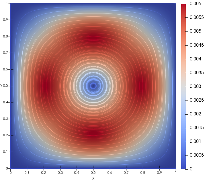
Figure 4.1: The streamlines and magnitudes of initial velocity field

In the implementation, we employ a decoupled and, linear, and energy stable finite element method recently proposed by [63]. For the reader’s convenience, the scheme is list in the appendix. Since there is no available analytical solutions of the sharp interface limits, we regard the numerical solution with the interfacial width $\epsilon=0.01$ as the reference solution for the comparison. To verify the convergence of the solution with respect to $\epsilon$, we vary $\epsilon$ gradually from $0.1$ to $0.0125$.

First of all, we consider the dynamics of a rounded square. To that end, we initiate the phase field as,

$$\varphi_{0}=\tanh\left(\frac{\left\|x-x_{c}\right\|_{4}-0.3}{\sqrt{2}\varepsilon}\right).$$

Here $x_{c}=\left(0.5,0.5\right)$ is the center of the rounded square and $\left\|x-x_{c}\right\|_{4}$ is the $l_{4}$-distance between the points $x$ and $x_{c}$. The initial profile of the phase field is shown in Fig. 4.2. In the figure, the red color stands for the fluid 1, the blue color stands for the fluid 2, and the black curve represents the zero-level set of reference phase function. The physical parameters are taken as $\eta=\sigma=1,$$m_{0}=1$,$\gamma=0.1$ in this first test case.

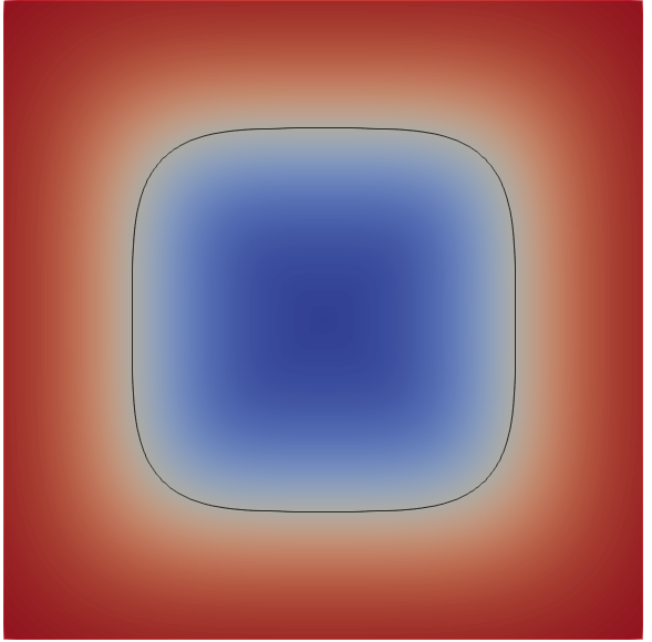
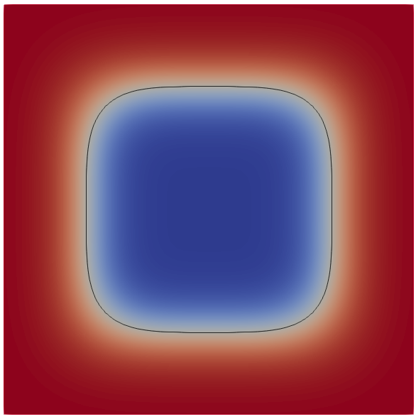
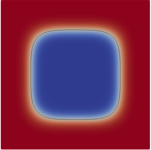
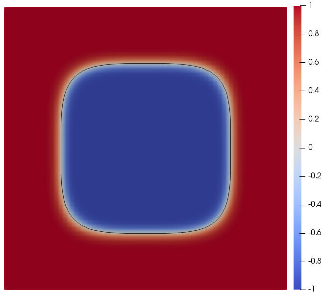
Figure 4.2: Initial initial profile of the phase field for $\epsilon=0.1,0.05,0.025,0.0125$.

Fig. 4.3 shows the snapshots of the two-phase interface at the final time $T=2.0$ in the simulation results for various mobilities and thickness. From this figure, we see that the isolated rounded square shape relaxes to a circular shape, due to the effect of surface tension for all cases. In order to see the convergence of the diffuse-interface model more clearly, we display the zero-level set of the computed phase function for different $\epsilon$ in Fig. 4.3. We observe that that as the width $\epsilon$ becomes smaller, the layers get thinner and converge to the black circle. Thus, it can be concluded that the diffuse-interface model converges to the sharp interface limits for all cases.

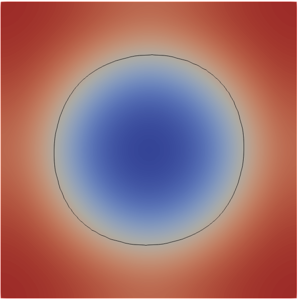
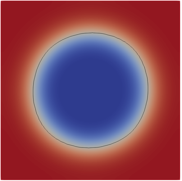
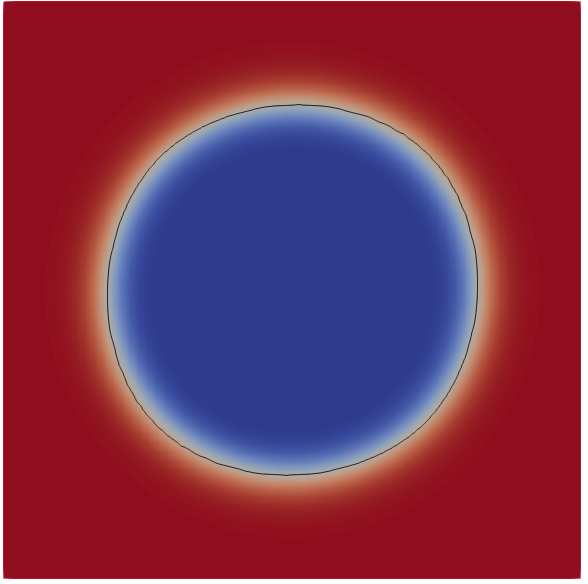
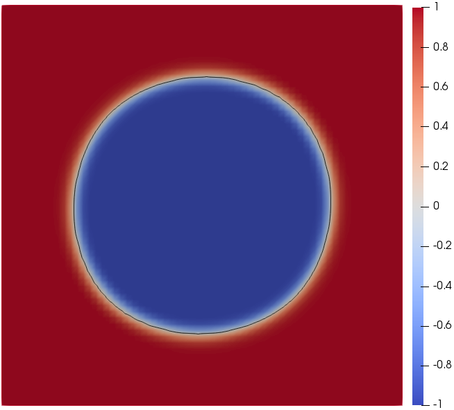
(a) Case I: $M\left(\varphi\right)=m_{0}$ .

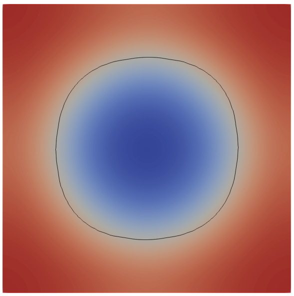
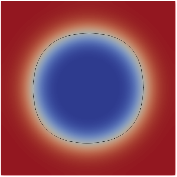
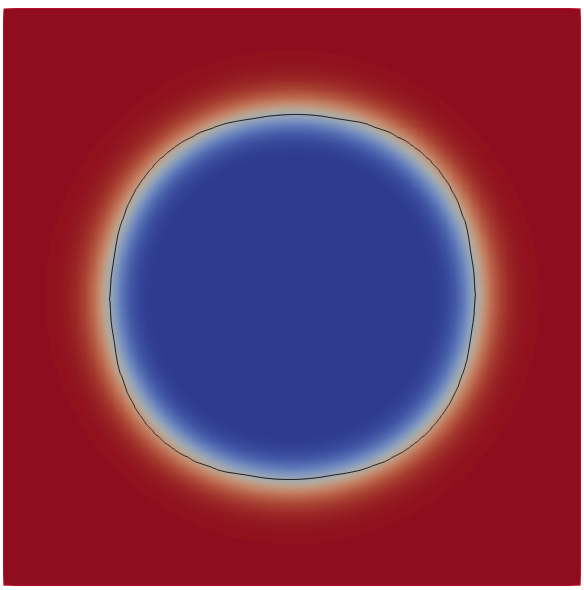
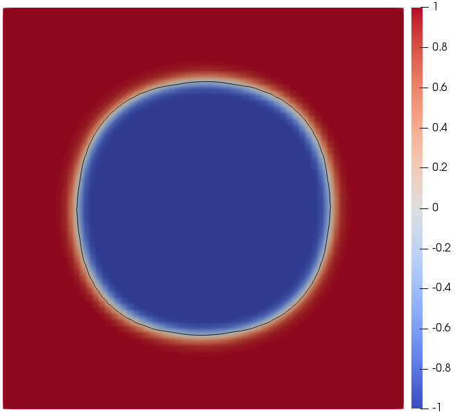
(b) Case II: $M\left(\varphi\right)=\epsilon m_{0}$.

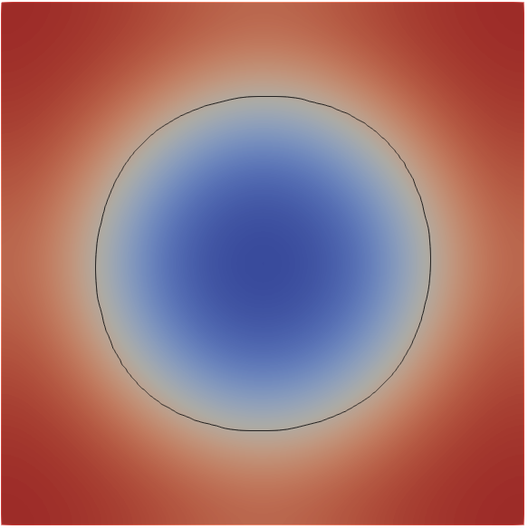
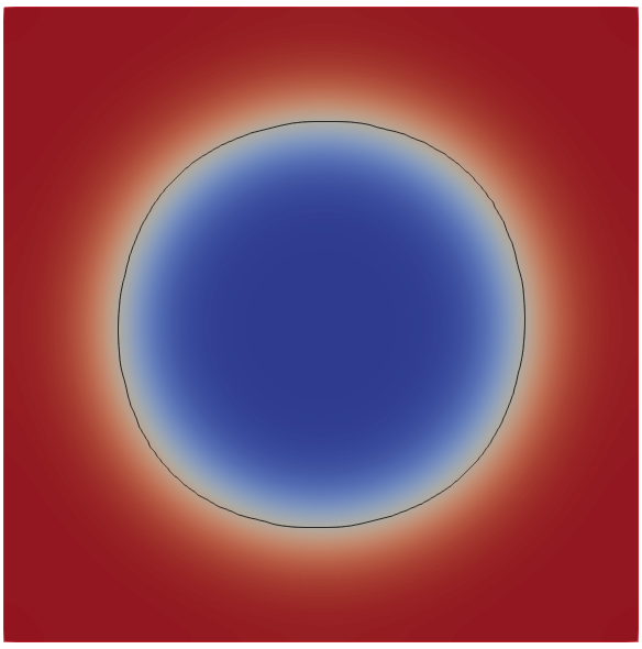
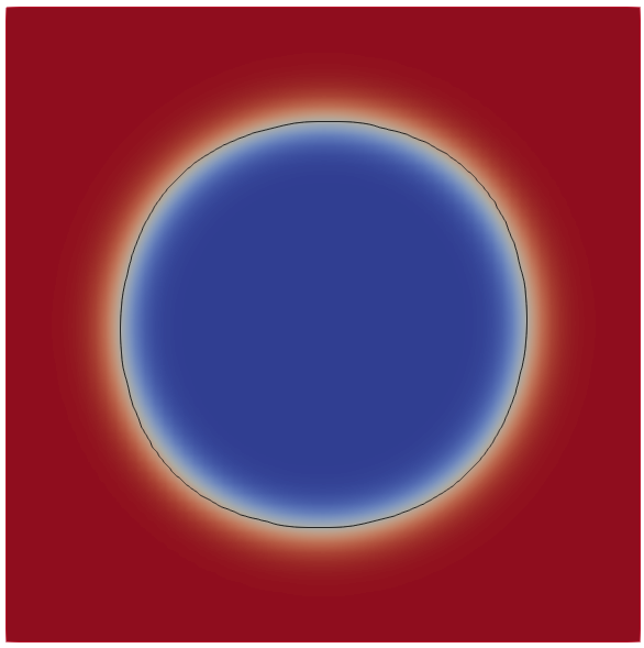
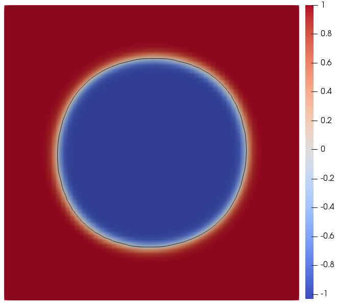
(c) Case III: $M\left(\varphi\right)=m_{0}\left(1+\varphi\right)_{+}^{2}$.

Figure 4.3: Profile of the phase fields for $\epsilon=0.1,0.05,0.025,0.0125$.(From left to right.)

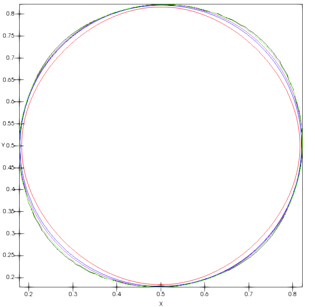
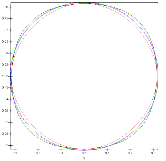
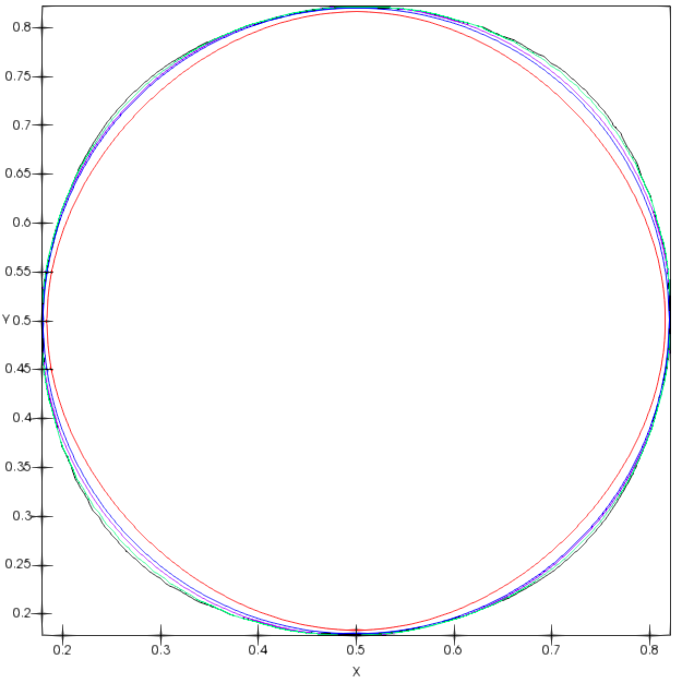
Figure 4.4: The zero-level set of the computed phase function for different $\epsilon$. Red: $\epsilon=0.1$, Blue: $\epsilon=0.05$, Purple: $\epsilon=0.025$, Blue: $\epsilon=0.0125$, Black: $\epsilon=0.01$.

Next, we consider the evolution of two separately inequal circular bubbles. The initial profile of phase function $\varphi$ is chosen to be

$$\varphi_{0}=1-\tanh\left(\frac{\left\|x-x_{o_{1}}\right\|-r_{1}}{\sqrt{2}\varepsilon}\right)-\tanh\left(\frac{\left\|x-x_{o_{2}}\right\|-r_{2}}{\sqrt{2}\varepsilon}\right)$$

where$\left\|x-x_{o_{i}}\right\|$ is the Eulerian distance between the points $x$ and $x_{o_{i}}$, $x_{o_{1}}=\left(0.3,0.5\right)$ and $x_{o_{2}}=\left(0.7,0.5\right)$ , are the center of two bubbles, $r_{1}=0.1,r_{2}=0.2$ are its radius. Fig. 4.5 displays the initial profile of the phase field. In this test case, the physical parameters are selected as $\eta=\sigma=100$,$m_{0}=\gamma=0.01$.

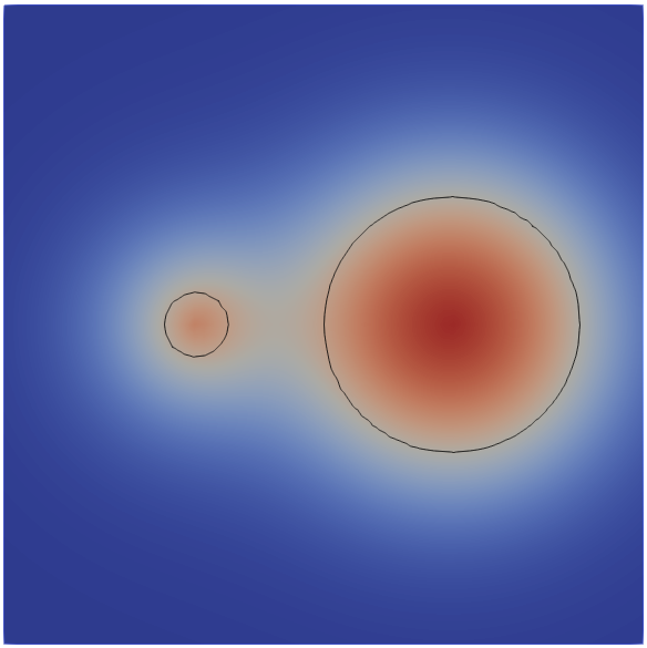
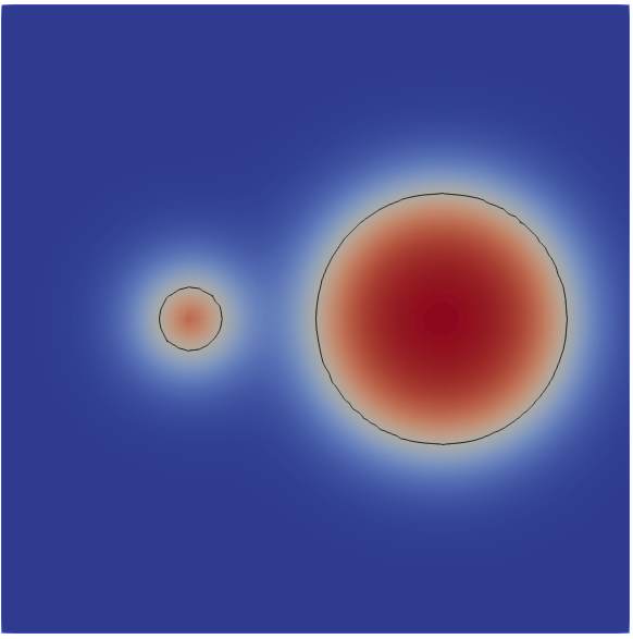
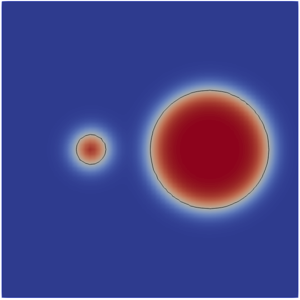
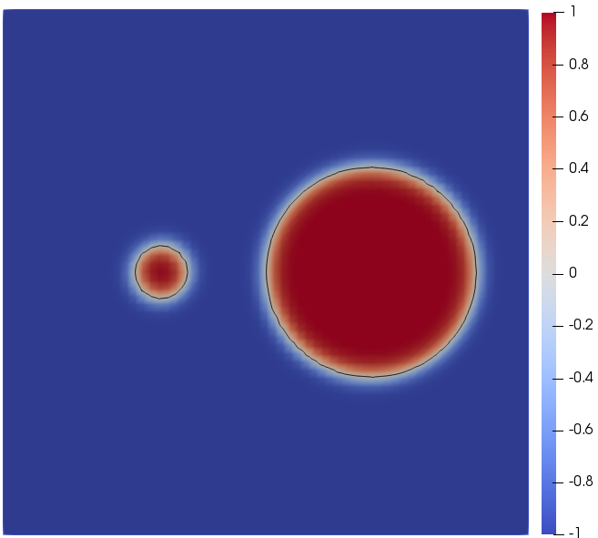
Figure 4.5: Initial initial profile of the phase field for $\epsilon=0.1,0.05,0.025,0.0125$.

We perform the experiments for this case as previous simulation. Fig. 4.6 displays the phase field obtained with the diffuse-interface model at the final time $T=2.5$ for various $\epsilon$. From this figure, one can see that the two bubbles eventually coalesces into a big bubble under the influence of surface tension for Cases I and III, while for Case II, two bubbles are still merging under the influence of surface tension. From these figure, one can see that the diffuse-interface models still converge towards their limits, even beyond the topological change which are not covered by the presented theory.

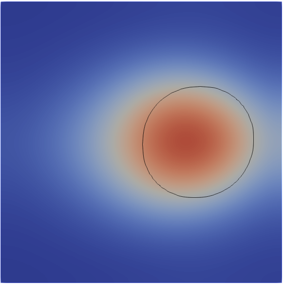
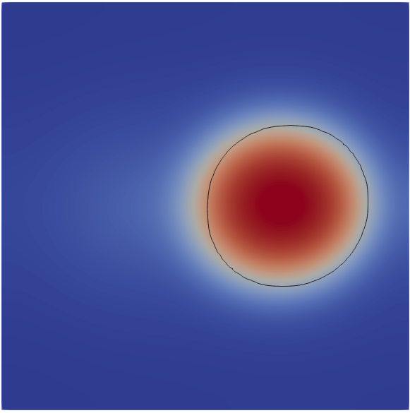
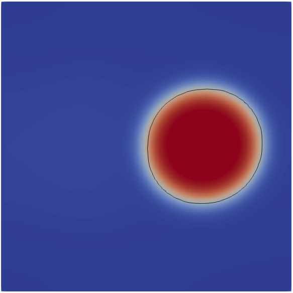
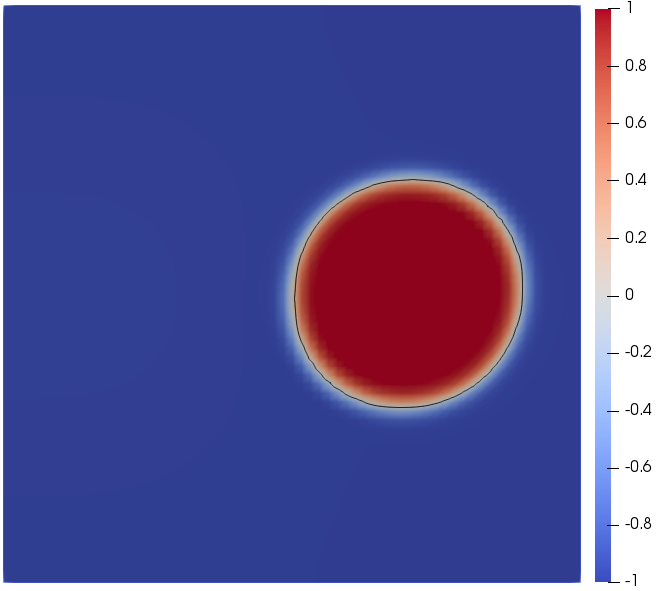
(a) Case I: $M\left(\varphi\right)=m_{0}$ .

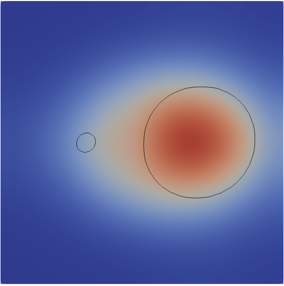
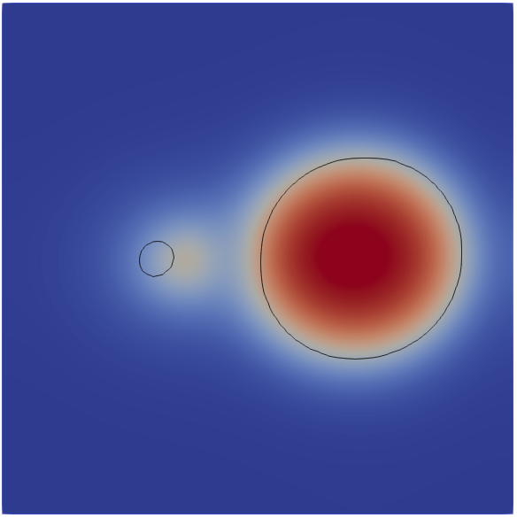
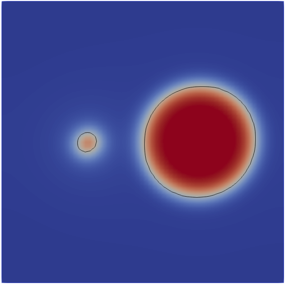
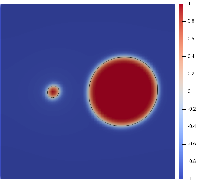
(b) Case II: $M\left(\varphi\right)=\epsilon m_{0}$.

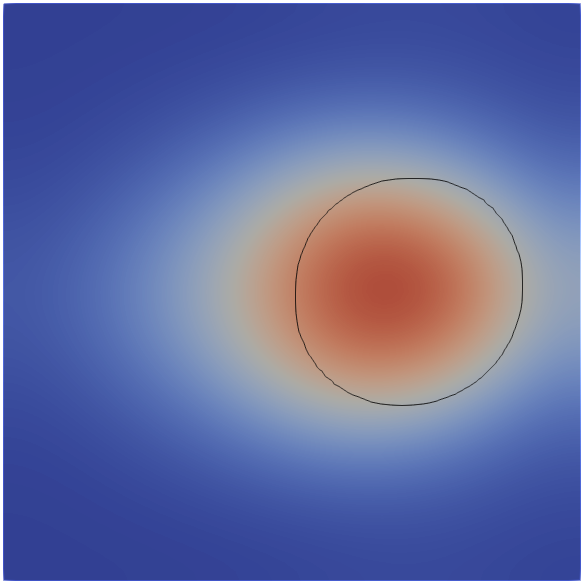
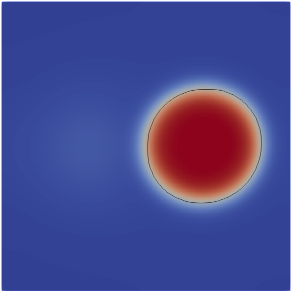
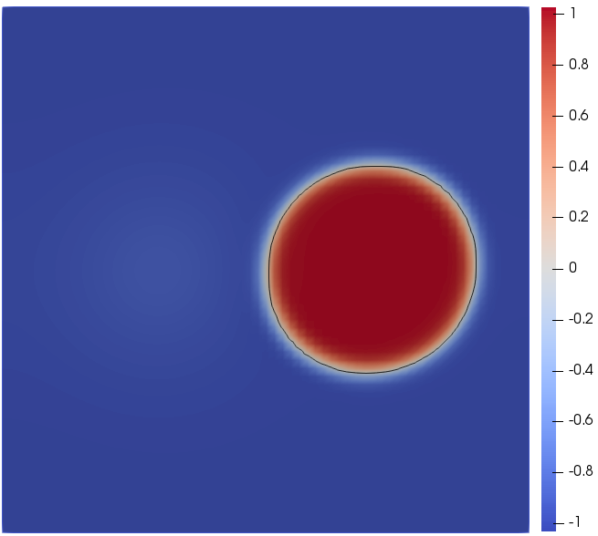
(c) Case III: $M\left(\varphi\right)=m_{0}\left(1+\varphi\right)_{+}^{2}$.

Figure 4.6: Profile of the phase fields for $\epsilon=0.1,0.05,0.025,0.0125$.(From left to right.)

5 Conclusions and remarks

In this paper, we propose and analyze a diffuse interface model for inductionless MHD fluids which couples a convective Cahn-Hilliard equation for the evolution of the interface, the Navier–Stokes system for fluid flow and the possion equation for electrostatics. The model is derived from Onsager’s variational principle and conservation laws systematically. Then we perform formally matched asymptotic expansions and develop several sharp interface limits for the diffuse interface model with different mobilitiess. Numerical results illustrate the convergence. Our analysis and numerical studies will be helpful in the real applications using the diffuse interface model for two-phase inductionless MHD fluids.

In upcoming works, we will investigate the model with large density ratio and the induced magnetic field. We also plan to study the highly efficient and energy stable schemes numerical methods for the corresponding models.

Appendix A CHiMHD model with moving contact lines

Moving contact line is a challenging problem in fluid dynamics. Here we give a sketch of an extension for the model (2.1) with moving contact lines. In the present case, the fluids is in contact with solid surfaces at $\Sigma$. Let $\gamma_{fs}\left(\phi\right)$ is the solid-fluid interfacial energy density (up to a constant), we add another term to the interfacial energy at the fluid-solid interface [29, 27],

$$E_{fs}=\int_{\Sigma}\gamma_{fs}(\varphi).$$

Then the total energy in this case takes the form,

$$E_{mcl}=E_{\varphi}+E_{\boldsymbol{u}}+E_{fs}.$$

The variational derivative of the energy $E_{mcl}$ with respect $\phi$ gives,

$$\delta E_{mcl}=\int_{\Omega}\mu\delta\varphi+\int_{\Sigma}L\delta\varphi,$$

with $L=\gamma_{fs}^{\prime}(\varphi)+\gamma_{0}\delta\frac{\partial\varphi}{\partial n}$ is a “chemical potential” on the boundary. For the boundary term, we introduce the material derivative at the boundary $\dot{\varphi}=\partial_{t}\varphi+\boldsymbol{u}_{\tau}\partial_{\tau}\varphi$,$\boldsymbol{u}_{\tau}$ is the tangential fluid velocity along the boundary tangential direction $\boldsymbol{\tau}$ and $\nabla_{\boldsymbol{\tau}}=\nabla-(\boldsymbol{n}\cdot\nabla)\boldsymbol{n}$ is the gradient along $\boldsymbol{\tau}$. With the similar arguments, one can get expression for the forces $\boldsymbol{F}$. The the dissipation function needs minor modifications,

$$\Phi\left(\mathbf{J},\mathbf{J}\right)=\int_{\Omega}\frac{\left|\boldsymbol{J}_{\varphi}\right|^{2}}{2M(\varphi)}+\int_{\Omega}\frac{|\boldsymbol{J}|^{2}}{2\sigma(\varphi)}+\int_{\Omega}\frac{|\mathbf{S}|^{2}}{2\eta(\varphi)}+\int_{\partial\Omega}\frac{\dot{\varphi}^{2}}{2\alpha^{-1}}+\int_{\partial\Omega}\frac{\beta}{2}\left|\boldsymbol{u}_{\tau}\right|^{2},$$ (A.1)

where $\mathbf{J}=\left(\mathbf{S},\boldsymbol{J}_{\varphi},\boldsymbol{J},\dot{\varphi},\boldsymbol{u}_{\tau}\right)$. Invoking with the Onsager’s variational principle, we find the boundary conditions for $\dot{\varphi}$ and $\boldsymbol{u}_{\tau}$ $\text{on }\Sigma$,

$$\alpha\dot{\varphi} =-L(\varphi)$$ (A.2)

$$\beta\boldsymbol{u}_{\tau} =-\eta(\varphi)(\mathbf{S}\boldsymbol{n})_{\tau}+L(\varphi)\partial_{\tau}\varphi.$$ (A.3)

The boundary condition for the tangential velocity is known as the generalized Navier boundary condition (GNBC) [59, 60]. Thus, we obtain the model with moving contact lines, adding the GNBC to the model (2.1).

Appendix B The numerical scheme

Let $\mathcal{T}_{h}$ be a quasi-uniform and shape-regular tetrahedral mesh of $\Omega$. As usual, we introduce the local mesh size $h_{K}=\mathrm{diam}\left(K\right)$ and the global mesh size $h:=\underset{K\in\mathcal{T}_{h}}{\max}h_{K}$. For any integer $k\geq 0,$ let $P_{k}(K)$ be the space of polynomials of degree $k$ on element $K$ and define $\boldsymbol{P}_{k}(K)=P_{k}(K)^{3}$. We employ the Mini-element to approximate the velocity and pressure

$$\boldsymbol{V}_{h}=\boldsymbol{P}_{1,h}^{b}\cap\boldsymbol{H}_{0}^{1}(\Omega),\quad Q_{h}=\left\{q_{h}\in H^{1}(\Omega)\cap L_{0}^{2}(\Omega):\left.q_{h}\right|_{K}\in P_{1}(K),\quad\forall K\in\mathcal{T}_{h}\right\}$$

where $P_{1,h}^{b}=\left\{v_{h}\in C^{0}(\Omega):\left.v_{h}\right|_{K}\in P_{1}(K)\oplus{\rm span}\{\hat{b}\},\;\forall K\subset T_{h}\right\}$, $\hat{b}$ is a bubble function. We choose the lowest-order Raviart-Thomas element space given by

$$\boldsymbol{D}_{h}=\left\{\boldsymbol{K}_{h}\in\boldsymbol{H}_{0}(\mathrm{div},\Omega):\left.\boldsymbol{K}_{h}\right|_{K}\in\boldsymbol{P}_{0}(K)+\boldsymbol{x}P_{0}(K),\quad\forall K\in\mathcal{T}_{h}\right\},$$

combined with the discontinuous and piecewise constant finite element space

$$S_{h}=\left\{\psi_{h}\in L_{0}^{2}(\Omega):\left.\psi_{h}\right|_{K}\in P_{0}(K),\quad\forall K\in\mathcal{T}_{h}\right\}.$$

The phase field $\phi$ and chemical potential $\mu$ are discretized by first order Lagrange finite element space $\left(X_{h},X_{h}\right)$,

$$X_{h}=\left\{\chi_{h}\in H^{1}(\Omega):\left.\chi_{h}\right|_{K}\in P_{1}(K),\quad\forall K\in\mathcal{T}_{h}\right\}.$$

Let $\left\{t_{n}=n\tau:\quad n=0,1,\cdots,N\right\},\tau=T/N,$ be an equidistant partition of the time interval $[0,T].$ For any time dependent function $\omega\left(x,t\right)$, the full approximation to $\omega\left(x,t_{n}\right)$ will be denoted by $\omega_{h}^{n}$. A fully discrete finite element scheme for problem (2.1) reads as follows: Given the initial datum $\boldsymbol{u}^{0}$ and $\phi^{0}$, we compute $\left(\boldsymbol{u}_{h}^{n+1},p_{h}^{n+1},\boldsymbol{J}_{h}^{n+1},\varphi_{h}^{n+1},\phi_{h}^{n+1},\mu_{h}^{n+1}\right)$, $n=0,1,\cdots,N-1$, by the following three steps:

Step 1: Find $\left(\varphi_{h}^{n+1},\mu_{h}^{n+1}\right)\in X_{h}\times X_{h}$ such that for any $\left(\psi_{h},\chi_{h}\right)\in X_{h}\times X_{h}$

$$\begin{cases}\left(\delta_{t}\varphi_{h}^{n+1},\psi_{h}\right)+\left(M(\varphi_{h}^{n})\nabla\mu_{h}^{n+1},\nabla\psi_{h}\right)+\tau\left(\varphi_{h}^{n}\nabla\mu_{h}^{n+1},\varphi_{h}^{n}\nabla\psi_{h}\right)&=\left(\varphi_{h}^{n}\boldsymbol{u}_{h}^{n},\nabla\psi_{h}\right),\\ \lambda\varepsilon\left(\nabla\varphi_{h}^{n+1},\nabla\chi_{h}\right)+\left(\frac{\lambda S}{\epsilon}(\varphi_{h}^{n+1}-\varphi_{h}^{n}),\chi_{h}\right)\\ +\left(\frac{\lambda}{\varepsilon}f(\varphi^{n}),\chi_{h}\right)-\left(\mu_{h}^{n+1},\chi_{h}\right)&=0,\end{cases}$$ (B.1)

Step 2: Find $\left(\boldsymbol{J}_{h}^{n+1},\varphi_{h}^{n+1}\right)\in\boldsymbol{D}_{h}\times S_{h}$ such that for any $\left(\boldsymbol{K}_{h},\theta_{h}\right)\in\boldsymbol{D}_{h}\times S_{h}$

$$\begin{cases}\left(\sigma\left(\varphi_{h}^{n+1}\right)^{-1}\boldsymbol{J}_{h}^{n+1},\boldsymbol{K}_{h}\right)+\tau\left(\boldsymbol{J}_{h}^{n+1}\times\boldsymbol{B},\boldsymbol{K}_{h}^{n+1}\times\boldsymbol{B}\right)\\ -\left(\phi_{h}^{n+1},\mathrm{div}\boldsymbol{K}_{h}\right)-\tau\left(\varphi_{h}^{n+1}\nabla\mu_{h}^{n+1}\times\boldsymbol{B},\boldsymbol{K}_{h}^{n+1}\right)&=\left(\boldsymbol{u}_{h}^{n}\times\boldsymbol{B},\boldsymbol{K}_{h}^{n+1}\right),\\ \left(\mathrm{div}\boldsymbol{J}_{h}^{n+1},\theta_{h}\right)&=0,\end{cases}$$ (B.2)

Step 3: Find $\left(\boldsymbol{u}^{n+1},p^{n+1}\right)\in\boldsymbol{V}_{h}\times Q_{h}$ such that $\left(\boldsymbol{v}_{h},q_{h}\right)\in\boldsymbol{V}_{h}\times Q_{h}$

$$\begin{cases}(\delta_{t}\boldsymbol{u}_{h}^{n+1},\boldsymbol{v}_{h})+\mathcal{O}(\boldsymbol{u}_{h}^{n},\boldsymbol{u}_{h}^{n+1},\boldsymbol{v}_{h})+2\left(\eta\left(\phi^{n+1}\right)D\left(\boldsymbol{u}_{h}^{n+1}\right),D\left(\boldsymbol{v}_{h}^{n+1}\right)\right)\\ \qquad-\left(p_{h}^{n+1},{\rm div}\boldsymbol{v}_{h}\right)+\left(\varphi_{h}^{n+1}\nabla\mu_{h}^{n+1},\boldsymbol{v}_{h}\right)-\left(\boldsymbol{J}_{h}^{n+1}\times\boldsymbol{B},\boldsymbol{v}_{h}\right)&=\boldsymbol{0},\\ \left(\mathrm{div}\boldsymbol{u}^{n+1},q_{h}\right)&=0,\end{cases}$$ (B.3)

with $\mathcal{O}(\boldsymbol{u},\boldsymbol{v},\boldsymbol{w})\coloneqq 1/2\left[(\boldsymbol{u}\nabla\cdot\boldsymbol{v},\boldsymbol{w})-(\boldsymbol{u}\nabla\cdot\boldsymbol{w},\boldsymbol{v})\right]$ for $\boldsymbol{u},\boldsymbol{v},\boldsymbol{w}\in\boldsymbol{V}$.

The scheme (B.1)-(B.3) can be proved to be unconditional energy stable and charge-conservative. The finite element method is implemented on the finite element software FreeFEM developed by Hecht et al. [64]. In all the simulations in this paper, we choose the meshsize $h=1/64$ and timestep $\tau=0.01$.

References

References

- [1] M. Abdou, A. Ying, N. Morley, K. Gulec, S. Smolentsev, M. Kotschenreuther, S. Malang, S. Zinkle, T. Rognlien, P. Fogarty, et al., On the exploration of innovative concepts for fusion chamber technology, Fusion Engineering and Design 2 (54) (2001) 181–247.
- [2] M. Abdou, D. Sze, C. Wong, M. Sawan, A. Ying, N. Morley, S. Malang, Us plans and strategy for iter blanket testing, Fusion Science and Technology 47 (3) (2005) 475–487.
- [3] P. A. Davidson, An introduction to magnetohydrodynamics, Cambridge Texts in Applied Mathematics, Cambridge University Press, Cambridge, 2001.
- [4] M.-J. Ni, J.-F. Li, A consistent and conservative scheme for incompressible MHD flows at a low magnetic Reynolds number. Part III: On a staggered mesh, J. Comput. Phys. 231 (2) (2012) 281–298.
- [5] L. Li, M. Ni, W. Zheng, A charge-conservative finite element method for inductionless MHD equations. Part II: A robust solver, SIAM J. Sci. Comput. 41 (4) (2019) B816–B842.
- [6] J.-F. Gerbeau, C. Le Bris, T. Lelièvre, Mathematical methods for the magnetohydrodynamics of liquid metals, Numerical Mathematics and Scientific Computation, Oxford University Press, Oxford, 2006.
- [7] J. Szekely, Fluid flow phenomena in metals processing, Academic Press, 1979.
- [8] N. B. Morley, S. Smolentsev, L. Barleon, Liquid magnetohydrodynamics - recent progress and future directions for fusion, Fusion Engineering and Design 51/52 (2000) 701–713.
- [9] D. D. Joseph, Y. Y. Renardy, Fundamentals of two-fluid dynamics. Part II, Vol. 4 of Interdisciplinary Applied Mathematics, Springer-Verlag, New York, 1993, lubricated transport, drops and miscible liquids.
- [10] D. D. Joseph, Y. Y. Renardy, Fundamentals of two-fluid dynamics. Part I, Vol. 3 of Interdisciplinary Applied Mathematics, Springer-Verlag, New York, 1993, mathematical theory and applications.
- [11] M. Sussman, K. M. Smith, M. Y. Hussaini, M. Ohta, R. Zhi-Wei, A sharp interface method for incompressible two-phase flows, J. Comput. Phys. 221 (2) (2007) 469–505.
- [12] V.-T. Nguyen, V.-D. Thang, W.-G. Park, A novel sharp interface capturing method for two- and three-phase incompressible flows, Comput. & Fluids 172 (2018) 147–161.
- [13] R. Samulyak, J. Du, J. Glimm, Z. Xu, A numerical algorithm for MHD of free surface flows at low magnetic Reynolds numbers, J. Comput. Phys. 226 (2) (2007) 1532–1549.
- [14] J. Zhang, M.-J. Ni, Direct simulation of multi-phase MHD flows on an unstructured Cartesian adaptive system, J. Comput. Phys. 270 (2014) 345–365.
- [15] J. Zhang, M.-J. Ni, Direct numerical simulations of incompressible multiphase magnetohydrodynamics with phase change, J. Comput. Phys. 375 (2018) 717–746.
- [16] H. Ki, Level set method for two-phase incompressible flows under magnetic fields, Comput. Phys. Comm. 181 (6) (2010) 999–1007.
- [17] W. X. Xie, L. Cai, J. H. Feng, Tracking entropy wave in ideal mhd equations by weighted ghost fluid method, Applied Mathematical Modelling 31 (11) (2007) 2503–2514.
- [18] M. E. Gurtin, D. Polignone, J. Viñals, Two-phase binary fluids and immiscible fluids described by an order parameter, Math. Models Methods Appl. Sci. 6 (6) (1996) 815–831.
- [19] C. Amrouche, C. Bernardi, M. Dauge, V. Girault, Vector potentials in three-dimensional non-smooth domains, Math. Methods Appl. Sci. 21 (9) (1998) 823–864.
- [20] J. W. Cahn, J. E. Hilliard, Free Energy of a Nonuniform System. I. Interfacial Free Energy and Free Energy of a Nonuniform System. III. Nucleation in a Two–Component Incompressible Fluid, John Wiley & Sons, Ltd, 2013.
- [21] S. M. Allen, J. W. Cahn, A microscopic theory for antiphase boundary motion and its application to antiphase domain coarsening, Acta Metallurgica 27 (6) (1979) 1085–1095.
- [22] C. Liu, An introduction of elastic complex fluids: an energetic variational approach, in: Multi-scale phenomena in complex fluids, Vol. 12 of Ser. Contemp. Appl. Math. CAM, World Sci. Publishing, Singapore, 2009, pp. 286–337.
- [23] C. Liu, J. Shen, A phase field model for the mixture of two incompressible fluids and its approximation by a Fourier-spectral method, Phys. D 179 (3-4) (2003) 211–228.
- [24] C. Liu, J. Shen, X. Yang, Decoupled energy stable schemes for a phase-field model of two-phase incompressible flows with variable density, J. Sci. Comput. 62 (2) (2015) 601–622.
- [25] H. Abels, E. Feireisl, On a diffuse interface model for a two-phase flow of compressible viscous fluids, Indiana Univ. Math. J. 57 (2) (2008) 659–698.
- [26] H. Abels, H. Garcke, G. Grün, Thermodynamically consistent, frame indifferent diffuse interface models for incompressible two-phase flows with different densities, Math. Models Methods Appl. Sci. 22 (3) (2012) 1150013, 40.
- [27] R. H. Nochetto, A. J. Salgado, S. W. Walker, A diffuse interface model for electrowetting with moving contact lines, Math. Models Methods Appl. Sci. 24 (1) (2014) 67–111.
- [28] R. H. Nochetto, A. J. Salgado, I. Tomas, The equations of ferrohydrodynamics: modeling and numerical methods, Math. Models Methods Appl. Sci. 26 (13) (2016) 2393–2449.
- [29] C. Eck, M. Fontelos, G. Grün, F. Klingbeil, O. Vantzos, On a phase-field model for electrowetting, Interfaces Free Bound. 11 (2) (2009) 259–290.
- [30] M. A. Fontelos, G. Grün, S. Jörres, On a phase-field model for electrowetting and other electrokinetic phenomena, SIAM J. Math. Anal. 43 (1) (2011) 527–563.
- [31] H.-G. Lee, J. S. Lowengrub, J. Goodman, Modeling pinchoff and reconnection in a Hele-Shaw cell. I. The models and their calibration, Phys. Fluids 14 (2) (2002) 492–513.
- [32] D. Han, D. Sun, X. Wang, Two-phase flows in karstic geometry, Math. Methods Appl. Sci. 37 (18) (2014) 3048–3063.
- [33] M. Fei, Global sharp interface limit of the Hele-Shaw-Cahn-Hilliard system, Math. Methods Appl. Sci. 40 (3) (2017) 833–852.
- [34] D. Hilhorst, J. Kampmann, T. N. Nguyen, K. G. Van Der Zee, Formal asymptotic limit of a diffuse-interface tumor-growth model, Math. Models Methods Appl. Sci. 25 (6) (2015) 1011–1043.
- [35] M. Ebenbeck, H. Garcke, Analysis of a Cahn-Hilliard-Brinkman model for tumour growth with chemotaxis, J. Differential Equations 266 (9) (2019) 5998–6036.
- [36] H. Garcke, K. F. Lam, E. Sitka, V. Styles, A Cahn-Hilliard-Darcy model for tumour growth with chemotaxis and active transport, Math. Models Methods Appl. Sci. 26 (6) (2016) 1095–1148.
- [37] J. Shen, Modeling and numerical approximation of two-phase incompressible flows by a phase-field approach, in: Multiscale modeling and analysis for materials simulation, Vol. 22 of Lect. Notes Ser. Inst. Math. Sci. Natl. Univ. Singap., World Sci. Publ., Hackensack, NJ, 2012, pp. 147–195.
- [38] Q. Du, X. Feng, Chapter 5 - the phase field method for geometric moving interfaces and their numerical approximations 21 (2020) 425 – 508.
- [39] T. Tao, Q. Zhonghua, Efficient numerical methods for phase-field equations, SCIENTIA SINICA Mathematica 50 (6) (2020) 775–794.
- [40] H. L. Liwei Ding, Yafei Cao, Z. Liu, Mhd numerical simulation of aluminum electrolytic cell (in chinese), Metal Materials and Metallurgy Engineering 42 (4) (2014) 8–13.
- [41] R. Chen, H. Zhang, Second-order energy stable schemes for the new model of the Cahn-Hilliard-MHD equations, Adv. Comput. Math. 46 (6) (2020) 79.
- [42] S. Mao, X. Wang, Fully discrete finite element approximation of a three-dimensional diffuse interface model for two-phase incompressible inductionless magnetohydrodynamic fluids, In preparation.
- [43] X. Feng, A. Prohl, Analysis of a fully discrete finite element method for the phase field model and approximation of its sharp interface limits, Math. Comp. 73 (246) (2004) 541–567.
- [44] M. Ebenbeck, H. Garcke, R. Nürnberg, Cahn-Hilliard-Brinkman systems for tumour growth, Discrete Contin. Dyn. Syst. Ser. S 14 (11) (2021) 3989–4033.
- [45] G. L. Aki, W. Dreyer, J. Giesselmann, C. Kraus, A quasi-incompressible diffuse interface model with phase transition, Math. Models Methods Appl. Sci. 24 (5) (2014) 827–861.
- [46] Lars, Onsager, Reciprocal relations in irreversible processes. ii., Physical Review 37.
- [47] Onsager, Lars, Reciprocal relations in irreversible processes. i. 37 (4) (1931) 405–426.
- [48] L. Onsager, S. Machlup, Fluctuations and irreversible processes, Phys. Rev. (2) 91 (1953) 1505–1512.
- [49] Novick-Cohen, Amy, [handbook of differential equations: Evolutionary equations] volume 4 || chapter 4 the cahn–hilliard equation (2008) 201–228.
- [50] A. Miranville, The Cahn–Hilliard Equation: Recent Advances and Applications, 2019.
- [51] A. Castellanos (Ed.), Electrohydrodynamics, Vol. 380 of CISM International Centre for Mechanical Sciences. Courses and Lectures, Springer-Verlag, Vienna, 1998, papers from the 7th IUTAM Summer School held in Udine, July 1996.
- [52] G. W. Hanson, A. B. Yakovlev, Electromagnetic fundamentals.
- [53] M.-J. Ni, R. Munipalli, P. Huang, N. B. Morley, M. A. Abdou, A current density conservative scheme for incompressible MHD flows at a low magnetic Reynolds number. II. On an arbitrary collocated mesh, J. Comput. Phys. 227 (1) (2007) 205–228.
- [54] S. Engblom, M. Do-Quang, G. Amberg, A.-K. Tornberg, On diffuse interface modeling and simulation of surfactants in two-phase fluid flow, Commun. Comput. Phys. 14 (4) (2013) 879–915.
- [55] P. A. Lagerstrom, Matched asymptotic expansions, Vol. 76 of Applied Mathematical Sciences, Springer-Verlag, New York, 1988, ideas and techniques.
- [56] G. Caginalp, P. C. Fife, Dynamics of layered interfaces arising from phase boundaries, SIAM J. Appl. Math. 48 (3) (1988) 506–518.
- [57] P. C. Fife, O. Penrose, Interfacial dynamics for thermodynamically consistent phase-field models with nonconserved order parameter, Electron. J. Differential Equations (1995) No. 16, approx. 49 pp.
- [58] H. Garcke, B. Stinner, Second order phase field asymptotics for multi-component systems, Interfaces Free Bound. 8 (2) (2006) 131–157.
- [59] X. Xu, Y. Di, H. Yu, Sharp-interface limits of a phase-field model with a generalized Navier slip boundary condition for moving contact lines, J. Fluid Mech. 849 (2018) 805–833.
- [60] X.-P. Wang, Y.-G. Wang, The sharp interface limit of a phase field model for moving contact line problem, Methods Appl. Anal. 14 (3) (2007) 287–294.
- [61] M. G. Bowler, Lectures on statistical mechanics, Pergamon Press, 1982.
- [62] K. Deckelnick, G. Dziuk, C. M. Elliott, Computation of geometric partial differential equations and mean curvature flow, Acta Numer. 14 (2005) 139–232.
- [63] X. Wang, X. Zhang, Decoupled energy stable finite element method for the diffuse interface model of two–phase inductionless magnetohydrodynamic fluids, In preparation.
- [64] F. Hecht, New development in freefem++, J. Numer. Math. 20 (3-4) (2012) 251–265.