Sample Efficient Social Navigation
Using Inverse Reinforcement Learning

Abstract

In this paper, we present an algorithm to efficiently learn socially-compliant navigation policies from observations of human trajectories. As mobile robots come to inhabit and traffic social spaces, they must account for social cues and behave in a socially compliant manner. We focus on learning such cues from examples. We describe an inverse reinforcement learning based algorithm which learns from human trajectory observations without knowing their specific actions. We increase the sample-efficiency of our approach over alternative methods by leveraging the notion of a replay buffer (found in many off-policy reinforcement learning methods) to eliminate the additional sample complexity associated with inverse reinforcement learning. We evaluate our method by training agents using publicly available pedestrian motion data sets and compare it to related methods. We show that our approach yields better performance while also decreasing training time and sample complexity.

I INTRODUCTION

In this paper, we present a new algorithmic formulation to allow a robot to learn a navigation policy directly by observing human examples. We use inverse reinforcement learning, but modify the formulation to provide advantages over prior work (including our own).

Recent work has demonstrated the potential of mobile robots that operate in human-inhabited social spaces, such as service robots for the elderly [1], as shopping assistants [2], and in the office environment [3].

Robotic navigation is a well-understood area of robotics and contains rich literature concerning efficient robotic movement in challenging environments under various constraints. For the subproblem referred to as “social navigation”, however, the need to account for socially appropriate behavior is often as important as efficiency [4]. This reflects the fact that integrating mobile robots into human social spaces goes beyond simple obstacle avoidance and actively acts in a way that makes humans nearby comfortable. Such socially aware policies act according to the socially acceptable navigation rules and closely mimic the behavior exhibited by humans.

Unfortunately, the guidelines for suitable social navigation are not readily codified algorithmically (despite several attempts), often leading to fragile threshold-dependent behavior, and are quite context-dependent. As such, it behooves a system to become able to infer appropriate socially-aware policies from observational data. One approach to this is to mimic the behavior of humans in the same context.

While reinforcement learning (RL) can lead to powerful solutions when the reward structure for the problem is well understood, social navigation depends on a range of poorly understood cues that may depend on the scenario. Indeed, the problem of reward engineering is a pivotal challenge to obtaining desired behavior out of any RL based controller. This limits the modeling power of any hand-crafted reward function for the sake of socially compliant navigation.

Ideally, the reward structure of socially compliant behavior would be learned from demonstrations of human pedestrians who already exhibit such socially compliant behavior. As such, inverse reinforcement learning (IRL) is attractive since it allows us to infer suitable rewards from raw features based on observations. A policy trained on these learned rewards using RL yields a suitable socially compliant navigation controller.

The IRL process, however, is typically computationally expensive and sample inefficient, partly due to the amount and quality of diverse demonstration data needed and due to the ill-posed nature of its mathematical formulation. These obstacles towards practical inverse reinforcement learning for social navigation are compounded by the difficulty of defining useful performance metrics to judge the performance of resulting algorithms and models (unsurprisingly, since robust and clear performance metrics could be used as optimization objectives).

In this paper, we present a model-free and sample efficient deep inverse reinforcement learning based navigation pipeline that can produce artificial agents that learn social navigation from observation. By leveraging existing trajectories within the replay buffer of off-policy RL algorithms, we eliminate the need for further environment interaction during the reward learning phase, yielding better sample efficiency and faster training. We evaluate the performance of our approach on metrics capturing desirable aspects of social navigation as well as its sample efficiency and compare against other approaches in the literature.

II RELATED WORK

A natural blueprint for human-aware navigation is to extend classical obstacle avoidance and navigation planning algorithms to fit the constraints of this new domain. One such approach is the reciprocal collision avoidance for pedestrians (RCAP) algorithm [4] which extends ORCA [5] by taking various human factors such as reaction time, physical constraints, and personal space into account. Müller et al. [6] extend A* [7] by identifying and following a leader until the social obstacle is overcome. Svenstrup et al. [8] propose a social path planning algorithm that models humans as dynamic obstacles with inviolable social zones enforced by a dynamic potential field optimized by rapidly exploring random trees (RRT) [9].

Pioneering work from Helbing and Molnar [10] models human behavior using repulsive forces exerted between agents in an environment and an attractive force towards the goal position. Since the model parameters require careful tuning, some researchers have used camera footage for calibration [11, 12], while others have made use of genetic algorithms to the same end [13]. These approaches, while succinct, cannot capture context-dependencies and the subtle behaviors humans exhibit.

Chen et al. [14] make use of RL to train a navigational policy using a hand-crafted reward function that incentivizes reaching the destination and penalizes undesirable collisions. This was improved upon by Everett et al. [15] which leveraged GPU processing to train multiple simulated agents in parallel, and an LSTM network [16] to compress the state information of an arbitrary number of adjacent agents into a fixed-size vector. [17] demonstrate that the RL approach has the ability to learn socially compliant behavior (specifically, a social norm of passing by the right side) using a carefully designed reward function that depends on the situational dynamics.

In practice, the choice of reward function can dramatically impact learning rate and quality. IRL has thus been used to learn reward functions directly from observations of human pedestrian traffic. A widely-used IRL framework is maximum entropy (MaxEnt) IRL [18] which allows the parameters of a reward function to be optimized using maximum likelihood estimation (MLE). Kitani et al. [19] apply a modified MaxEnt IRL [18] model to forecast pedestrian trajectories from noisy camera data which can also double as a navigation controller.

Vasquez et al. [20] investigate composite features leveraging the motion information of nearby pedestrians and demonstrate that IRL learned reward parameters are superior to manually tuned ones. Henry et al. [21] use Gaussian processes (GP) to estimate environment features from incomplete data and use rewards learned from MaxEnt IRL as A* heuristics for path planning, quantitatively demonstrating a more human-like quality to the chosen trajectories.

Kretzschmar et al. [22], building on previous work [23, 24], apply a maximum entropy approach to learn a joint trajectory distribution of all navigating agents in an environment, including the robot itself. Inference over the spline-based trajectory representation is made possible by heuristically sampling high probability regions from certain defined homotopy classes. This approach is tested on a real robot in an overtake scenario [23] and demonstration data collected from four pedestrians in an enclosed environment [24] and a dataset [25] of three to five pedestrians. While learning a joint distribution over all agents allows for high-quality inference, it does not scale to moderately populated settings (e.g. a few dozen agents).

An alternative probabilistic approach to IRL, Bayesian IRL (BIRL), is proposed by Ramachandran et al. [26] where the reward is modeled as a random variable vector that dictates the distribution of expert states and actions. The distribution over the rewards which best explains expert trajectories is then inferred.

Okal et al. [27] use a modified BIRL approach using control graphs [28] to tractably capture continuous state information via macrostates in a graph-based representation. Since a graph-based representation is learned, local controllers can be used in conjunction with global planning algorithms such as RRT or A* using the learned rewards for navigation, as the authors demonstrate both in a simulation of artificial pedestrians and via a real robot. Kim et al. [29] use BIRL to learn a linear reward function over features extracted from RGB-D cameras on a robotic wheelchair, which are then used for path planning purposes in crowded environments.

The linear reward function used by MaxEnt IRL [18] struggles with complex non-linear rewards. To address this, Wulfmeier et. al [30] introduce maximum entropy deep inverse reinforcement learning (MEDIRL), extending MaxEnt IRL to deep neural network based reward functions. Fahad et al. [31] leverage MEDIRL and velocity-augmented SAM features [32] to train a navigation policy on pedestrian data in a grid world setting. Konar et al. [33] propose deterministic MEDIRL (det-MEDIRL), which efficiently learns goal conditioned navigation policies using a risk-based feature representation that segments the agent’s surrounding pedestrians based on the posed collision risk. These approaches require many costly policy roll-outs at each iteration of the reward function optimization, which greatly slows down training.

III INVERSE REINFORCEMENT LEARNING

We begin by outlining IRL-based learning for social navigation, and then describe how we enhance it. A Markov decision process (MDP) $\mathcal{M}$ is defined by the tuple $(\mathcal{S},\mathcal{A},\mathcal{T},R,\gamma,p_{0})$ where $\mathcal{S}$ is the set of possible states, $\mathcal{A}$ is the set of possible actions, transition probabilities $\mathcal{T}(s,a,s^{\prime})=P(s^{\prime}=s_{t+1}|s=s_{t},a=a_{t})$ modelling the probability of transitioning from state $s_{t}$ to $s_{t+1}$ by taking action $a_{t}$. $R:\mathcal{S}\mapsto\mathbb{R}$ is the reward function, $\gamma$ is the discounting factor, and $p_{0}=P(s=s_{0})$ is the probability distribution of possible initial states.

An observed trajectory $\tau$ of length $t$ is any valid ordered sequence of states where $s_{i}\in\mathcal{S}$.

$$\tau_{obs}=\left\{s_{0},s_{1},\dots,s_{t}\right\}$$

In this work, we are learning from observation (LfO) as opposed to learning from demonstration (LfD) as we do not assume access to the actions of the expert. This distinction is important since, among other factors, action selection includes non-determinism and often a significantly different action space between expert and robot. Due to the lack of action information, LfO is a harder problem to solve [34].

A (stochastic) policy is a mapping $\pi:\mathcal{S}\times\mathcal{A}\mapsto[0,1]$. For an agent which obtains rewards through environment interaction, reinforcement learning (RL) is the process of finding an optimal policy $\pi^{*}$ from the set of admissible policies $\Pi$ that maximizes the discounted total returns.

$$\pi^{*}=\operatorname*{arg\,max}_{\pi\in\Pi}\operatorname{\mathbb{E}}_{\tau\sim\pi}\left[\sum_{s_{t},a_{t}\in\tau}\gamma^{t}R(s_{t},a_{t},s^{\prime}_{t})\right]$$ (1)

The goal of inverse reinforcement learning (IRL) is to determine the optimal reward function $R^{*}$ which an expert policy $\pi_{E}$ is presumably optimizing. That can be seen as a reward-based explanation for the observed behavior. In our case, this would be computed over trajectories $D=\{\tau_{1},\tau_{2},\dots,\tau_{M}\}$ from the expert policy.

We use the MaxEnt IRL framework [18, 35], which assumes a maximum entropy distribution over the trajectory space

$$P(\tau|\bm{\theta})=\frac{1}{Z(\bm{\theta})}\exp(R_{\bm{\theta}}(\tau))$$ (2)

where $R_{\bm{\theta}}$ is a reward function with parameters $\bm{\theta}$, and $Z(\bm{\theta})$ is the partition function. With a differentiable reward function and a convergent partition function, MLE can be used to fit this distribution to a set of expert observation trajectories $D_{E}$. While prior work derives a state visitation frequency (SVF) based derivative [33, 31], we use importance sampling to estimate the partition function following guided cost learning (GCL) [36]

$$Z(\bm{\theta}) =\int_{\tau}\exp(R_{\theta}(\tau))d\tau\approx\operatorname*{\mathbb{E}}_{\tau\sim q(\tau)}\frac{\exp(R_{\theta}(\tau))}{q(\tau)}$$ (3)

With this approximation, the MaxEnt log-likelihood becomes

$$L(\bm{\theta})\approx\operatorname*{\mathbb{E}}_{\tau_{E}\in D_{E}}R_{\bm{\theta}}(\tau_{E})-\log\operatorname*{\mathbb{E}}_{\tau\sim D_{q}}\frac{\exp(R_{\bm{\theta}}(\tau))}{q(\tau)}$$ (4)

GCL uses a policy trained on the current rewards as the sampling policy $q(\tau)$, thus minimizing the variance of the importance sampling estimator [36] The training of the policy is interleaved with the rewards function, removing RL as inner-loop component and greatly accelerating training. In practice, however, simply using the latest iteration policy is impractical due to the initially poor coverage. As such, a mixture distribution $\mu(\tau)=\frac{1}{2}\pi(\tau)+\frac{1}{2}\hat{q}(\tau)$ is used as sampling distribution, where $\hat{q}(\tau)$ is a crude approximate distribution over the expert trajectories [36, 37].

The MaxEnt IRL framework learns rewards that induce policies that match the expert features. For social navigation, we use risk features [33] that encode relative pedestrian locations and change in velocity which should lead to a less intrusive policy with smoother trajectories when applied to social navigation, as well as features orienting the agent towards the goal position, which should lead to collision-free navigation.

IV Improving Sample Efficiency

An important technique in off-policy RL is the use of experience replay buffers [38] to boost sample efficiency by way of re-using old experiences for training. In our method, which we call “ReplayIRL”, we make use of soft actor critic (SAC), a recent sample-efficient RL algorithm [39, 40]. We further increase the sample efficiency of our algorithm by reusing the trajectories collected in the replay buffer as samples for the importance sampling calculation of the reward log-likelihood, an approach that was previously employed in the related imitation learning domain [41].

We use an alternative formulation of the GCL log-likelihood (4) by Fu et al. [42] as it is more stable, and includes discounting while using a state-only reward function formulation.

$$L_{obs}(\bm{\theta})=\operatorname*{\mathbb{E}}_{\tau\sim D_{E}}\left[\sum_{s_{t}\in\tau}\gamma^{t}R_{\bm{\theta}}(s_{t})\right]$$ (5)

$$L_{IS}(\bm{\theta})=\operatorname*{\mathbb{E}}_{\tau\sim\mu}\left[\sum_{s_{t},a_{t}\in\tau}\log(e^{\gamma^{t}R_{\bm{\theta}}(s_{t})}+\pi(a_{t}|s_{t}))\right]$$ (6)

$$L(\bm{\theta})=L_{obs}(\bm{\theta})-L_{IS}(\bm{\theta})$$ (7)

We modify the above equations to sample from a replay buffer $B$ instead of performing policy roll-outs. Additionally, we share the expert trajectory samples for the calculation of both $L_{obs}$ and $L_{IS}$. This results in a mixture distribution

$$\hat{\mu}(\tau)=\frac{1}{2}D_{E}(\tau)+\frac{1}{2}B(\tau)$$ (8)

where we slightly overload notation by treating the replay buffer $B$ and expert trajectories $D_{E}$ as distributions. In practice, we simply uniformly sample trajectories from both collections.

Note that in (6), the quantity $\pi(a|s)$ cannot be evaluated for expert trajectories as their actions are unknown. We found that letting $\pi(a|s)=\frac{1}{\sigma_{T}\sqrt{2\pi}}$, a constant value, is sufficient for training. This crude approximation corresponds to the density of a Gaussian policy with target standard deviation $\sigma_{T}$ at the mean value.

Following the above modifications, the importance sampling portion of the algorithm becomes

$$A(\bm{\theta},\tau)=\begin{cases}\sum\limits_{s_{t},a_{t}\in\tau}\log(e^{\gamma^{t}R_{\bm{\theta}}(s_{t})}+\pi(a_{t}|s_{t}))&\tau\in B\\ \sum\limits_{s_{t},a_{t}\in\tau}\log(e^{\gamma^{t}R_{\bm{\theta}}(s_{t})}+\frac{1}{\sigma_{T}\sqrt{2\pi}})&\tau\in D_{E}\end{cases}$$ (9)

$$\hat{L}_{IS}(\bm{\theta},\tau_{B})=\operatorname*{\mathbb{E}}_{\tau\in\tau_{B}}\left[A(\bm{\theta},\tau)\right]$$ (10)

$$\hat{L}_{obs}(\bm{\theta},\tau_{E})=\operatorname*{\mathbb{E}}_{\tau\in\tau_{E}}\left[\sum_{s_{t}\in\tau}\gamma^{t}R_{\bm{\theta}}(s_{t})\right]$$ (11)

where we use $\tau_{B}$ and $\tau_{E}$ as placeholders for appropriately sampled sets of trajectories passed to these functions, since in practice these trajectories are sampled before computing the above quantities. Finally, we use SAC with automatic entropy tuning [40], and update the rewards of the sampled batch, ensuring that SAC will perform updates with the up-to-date reward function. The full algorithm can be found in Algorithm 1.

Input : expert demonstrations $D_{E}$
maximum iterations $M$
training intervals $i_{RL}$, $i_{IRL}$

Output : optimized parameter $\bm{\theta}$ and policy $\pi$

Procedure UpdateReward()

       sample $n_{E}$ expert trajectories $\tau_{E}\sim D_{E}$

       sample $n_{B}$ replay buffer trajectories $\tau_{B}\sim B$

       $\tau_{B}\leftarrow\tau_{B}\cup\tau_{E}$

       $\hat{L}(\bm{\theta})\leftarrow\nabla_{\bm{\theta}}\left(\hat{L}_{obs}(\bm{\theta},\tau_{E})-\hat{L}_{IS}(\bm{\theta},\tau_{B})\right)$

       $\bm{\theta}\leftarrow\bm{\theta}-\alpha\nabla_{\bm{\theta}}L(\bm{\theta})$

      

Procedure UpdatePolicy()

       execute $\pi(a|s)$ to obtain $(s_{t},a_{t},s_{t+1})$

       $B\leftarrow B\cup(s_{t},a_{t},s_{t+1})$

       $B_{R}\leftarrow$ sample batch $(s_{t},a_{t},s_{t+1},R_{\bm{\theta}}(s_{t+1}))$

       update $\pi$ using SAC iteration using $B_{R}$

      

begin

       Initialize $\bm{\theta}\leftarrow\bm{\theta}_{0}$, $B\leftarrow\emptyset$

       for $m=1$ to $M$ do

             if $m\mod i_{RL}$ then

                   UpdatePolicy()

            if $m\mod i_{IRL}$ then

                   UpdateReward()

            

      

Algorithm 1 Replay IRL

V Experiments

We compare ReplayIRL to a recent deep IRL social navigation method, det-MEDIRL [33], as well as SAC trained on hand-crafted rewards. We use the UCY dataset [43] both as expert trajectories for training as well as for pedestrian placement in our simulated environment.

V-A Pedestrian Dataset Processing

The UCY dataset [43] is composed of five subsets students001, students003, zara01, zara02, and zara03. We concatenate the zara01-03 subsets into one, resulting in three distinct subsets students001, students003, and zara. The former two are from a mid-density public space in a university campus, while the latter is a lower-density sidewalk. The per-frame pedestrian positions and approximate gaze direction are provided, of which we only make use of the former.

We make use of an approximate homography to transform the overhead view from which the original data was collected into a top-down view. As a side effect, this also allows us to roughly convert the pixel space coordinates to world space.

We also removed inaccessible regions, trajectories that exhibited collisions, and other anomalous observations. The final pedestrian count is 365, 341, and 443 pedestrians in the students001, students003, and zara data sets respectively.

((a)) students001 subset.

((b)) Zara subset.

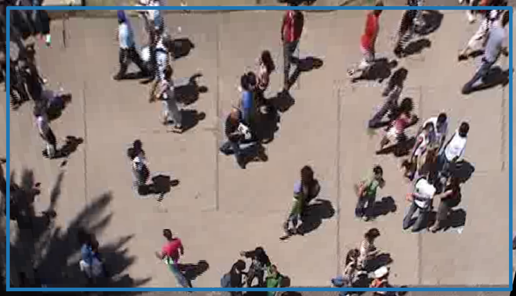
((c)) students001 subset.

((d)) Zara subset.

(x

Figure 1: (a) and (b) show ROI with blue bounding box in UCY locations [43]. (c) and (d) show corresponding corrected top-down approximation via homography.

V-B Simulation Environment

We implement a simulation environment to allow our agent to train in a crowded environment. We model pedestrians as discs with a diameter of $0.2\>m$ and position them according to the dataset. The continuous action space consists of the target forward speed in the range $[0,1.5]\>m/s$, and change in heading angle limited to the range $[0,\frac{3\pi}{2}]\>\text{deg}/s$. The agent is deterministically displaced based on its resulting velocity vector. Each simulator time step advances time by $0.04s$. For states, we compute risk features [33] which encode collision risk from nearby pedestrians. We use $0.65\;m$ and $1.0\;m$ as the radius of the inner and outer circles.

When each episode starts, a pedestrian is removed from the simulation for the duration of the experiment and replaced by the agent. The goal position of the agent is the final position of the removed pedestrian. The episode terminates when the agent is in the $10\;cm$ radius of the goal coordinates or after a $40\>s$ (1000 time step) timeout.

V-C Training details

We use a 2-layer fully connected deep neural network with 256 and 128 neurons per layer to represent the policy and reward networks respectively. We make use of the ReLU activation function [44] in both networks, and make use of the AdamW optimizer [45] with $l2$ weight decay of $10^{-4}$, learning rate of $10^{-4}$ for the reward network and $3\cdot 10^{-4}$ for SAC, learning rate decay $\gamma=0.9999$, reward update interval $i_{IRL}=3$, policy update interval $i_{RL}=1$, number of expert and policy samples $n_{E}=n_{B}=16$, 512 replay buffer samples for SAC. Other hyperparameters for SAC are the same as in [40].

We compare our algorithm with another deep IRL based social navigation algorithm, det-MEDIRL. We slightly modify det-MEDIRL to use SAC and batch gradient descent with the same batch size as ReplayIRL. This reduces the training time of det-MEDIRL from 72 to roughly 28 wall-time hours and while increasing sample efficiency without affecting the original performance (see section VI).

We also compare against a baseline SAC agent with hand-crafted rewards based on [15] with a shaped reward to help the agent reach the goal. The reward structure can be decomposed into the following components:

$$R_{\text{approach}}=0.1\times\frac{\Delta x\cdot d_{rg}}{||d_{rg}||_{2}}$$ (12)

$$R_{G}=\begin{cases}1&\text{if}~{}||x_{r}-x_{g}||_{2}\leq r_{g}\\ 0&\text{else}\end{cases}$$ (13)

$$R_{\text{col}}=\begin{cases}-1&\text{if}~{}d_{min}<2\cdot r_{ped}\\ -0.01\times d_{min}&\text{if}~{}d_{min}<4\cdot r_{ped}\end{cases}$$ (14)

Where $x_{t}$ and $x_{t-1}$ are the current and previous robot locations respectively, $\Delta x=x_{t}-x_{t-1}$ is the displacement vector, $x_{g}$ and $r_{g}$ are the goal location and radius respectively, $d_{min}$ is the distance to the nearest pedestrian, and $r_{ped}$ is the radius of the disc that models pedestrians. The total reward is then calculated $R=R_{\text{approach}}+R_{\text{col}}+R_{G}$.

We train ReplayIRL for $1.3\cdot 10^{5}$ iterations, det-MEDIRL for 2,000 iterations, and SAC for $4\cdot 10^{5}$ iterations. Every training experiment is carried out over 5 random seeds. All methods are trained on the student001 dataset and evaluated on student003 and zara datasets.

VI RESULTS

We evaluate the trained social navigation policies based on metrics that would, together, capture desirable aspects of social navigation. For every pedestrian in the test datasets (student003 and zara), we collect a trajectory by replacing said pedestrian with the agent. We repeat this for every starting position (i.e. every pedestrian). Furthermore, we collect metrics comparing the sample efficiency of the IRL based algorithms. Error bars and shaded areas represent 95% confidence interval in all figures.

VI-A Performance Results

VI-A1 Proxemic Intrusions

Informed by proxemics [46], we record the number of intimate and personal space intrusions. At each evaluation time step, for every pedestrian, the corresponding intrusion count is incremented should their mutual distance fall within the thresholds $[0,0.5]\;m$ and $(0.5,1.2]\;m$ for intimate and personal distance respectively.

Results in Figure 2 show that our method has the lowest proxemic intrusions out of all three compared methods on both test subsets, while SAC significantly exceeds the expert ground truth. Interestingly, both det-MEDIRL and ReplayIRL have lower proxemic intrusions than the ground truth, possibly because group behavior (which causes many such intrusions) is not considered by the solitary agents, which prefer a less intrusive policy to avoid the collision penalty.

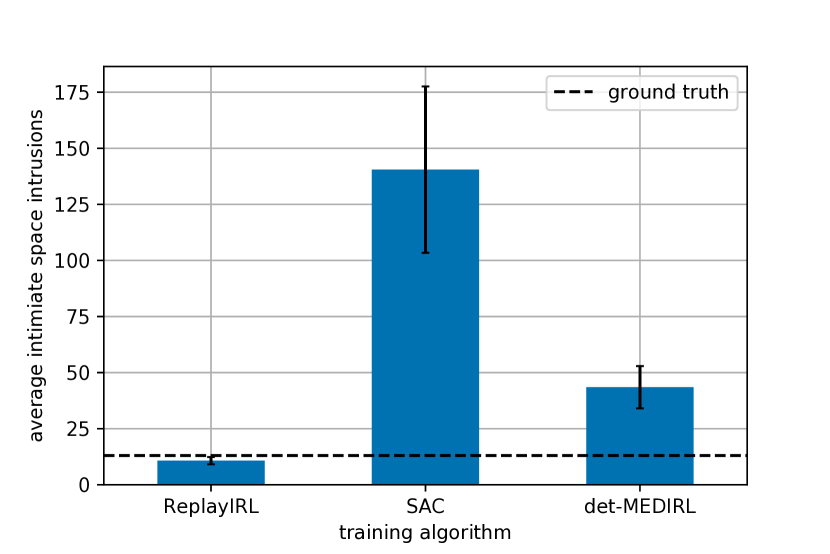
((a)) students003 subset.

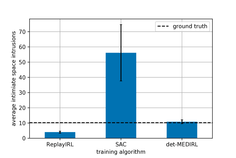
((b)) Zara subset.

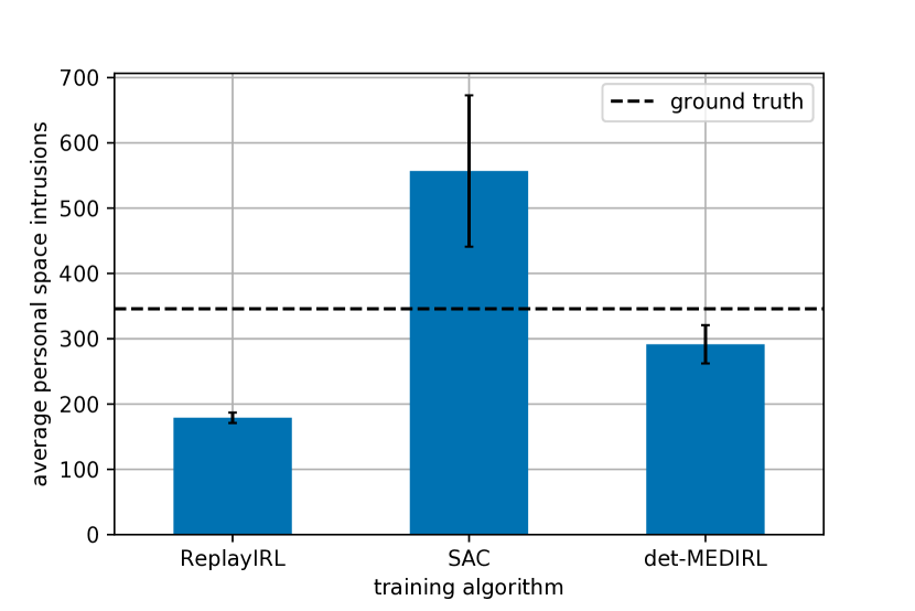
((c)) students003 subset.

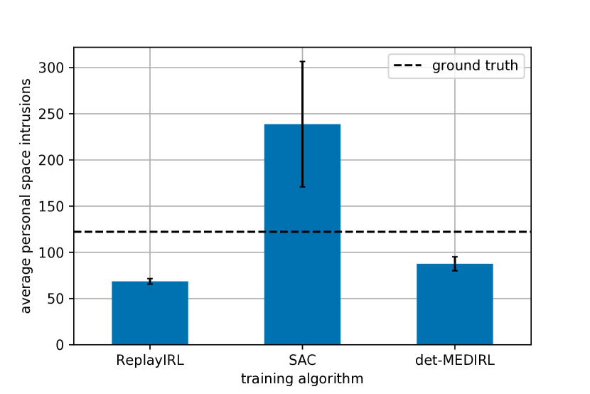
((d)) Zara subset.

Figure 2: Out of distribution intimate (a,b) and personal space (c,d) intrusions. The IRL methods are both less intrusive than ground truth, indicating that a conservative policy for solitary agents was learned.

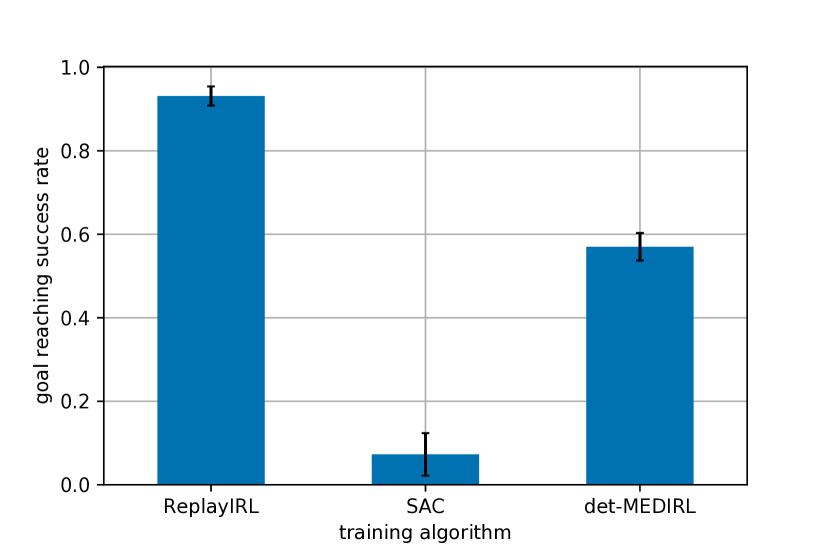
((a)) students003 subset.

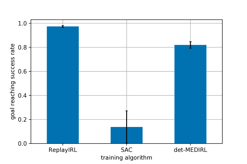
((b)) Zara subset.

Figure 3: Out of distribution goal reaching success rate. ReplayIRL is better at collision-free navigation than det-MEDIRL while SAC fails to learn collision-free navigation.

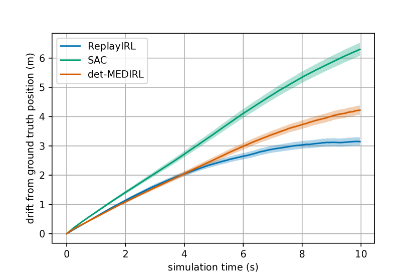
((a)) students003 subset.

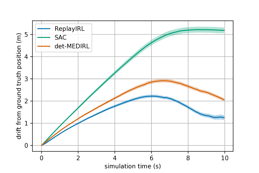
((b)) Zara subset.

Figure 4: Out of distribution average drift distance from ground truth position. ReplayIRL clearly stays closer to ground truth position than det-MEDIRL while SAC is completely divergent.

VI-A2 Drift from Ground Truth

This measure calculates the average $l2$ distance from the ground truth position of the replaced pedestrian for the first $10\,s$ of simulation. Results in Figure 4 clearly illustrate that ReplayIRL stays closer to the ground truth position despite the limited nature of the risk features it uses. From 4(b) at roughly $t=6\,s$ we can see that det-MEDIRL and ReplayIRL are influenced similarly by the configuration of surrounding pedestrians indicating some similarity in the extracted reward in IRL methods, while SAC is completely divergent.

VI-A3 Goal Reaching Success Rate

This metric measures the basic successful navigation and is defined as reaching the target goal location without collision with any other pedestrian. Results in Figure 3 illustrate that ReplayIRL is convincingly superior to det-MEDIRL in terms of performance, while SAC seems to fail to learn using hand-crafted rewards. This shows that the learned reward function is beneficially shaped to accelerate the RL learning process. We leave the investigation of this interesting RL acceleration effect to future work.

While det-MEDIRL achieves slightly better performance than the original implementation [33], ReplayIRL performs significantly better in both the students003 and zara subsets, which can be attributed to an improved reward function due to importance sampling and accelerated training speed which leads to more IRL learning iterations.

VI-B Sample Efficiency Results

VI-B1 Feature Matching

We record the root mean square error (RMSE) between the average expert state vector and the average policy state vectors at each training step as a measure of similarity between the agent and expert trajectories. For ReplayIRL, the trajectory sample from the replay buffer is used for this comparison. For presentation clarity, we use a moving average with a window size of 100 when visualizing results in Figure 5. The results in Figure 5 illustrate that ReplayIRL converges to an RMSE minimum in $\sim 10^{5}$ environment interactions, while det-MEDIRL has just begun to converge at $10^{7}$ environment interactions. This achieves a two order of magnitude reduction in the number of required environment interactions. While we leave the application of ReplayIRL on a robotic platform to future work, these results reinforce the practicality of such an endeavor.

We attribute this stark difference in sample efficiency to the density of IRL updates in ReplayIRL; the training speed and sample efficiency are greatly increased as the IRL subroutine does not require environment interaction. Note that while sample efficiency is more important for robot training, the training speed is also dramatically improved, down from 28.4 hours for det-MEDIRL to 7.2 hours for ReplayIRL as measured by wall time.

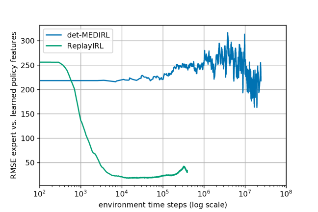
Figure 5: RMSE between average expert and replay buffer samples, measuring feature matching capability. The lower error shows better matching and the more rapid convergence of ReplayIRL is evident. det-MEDIRL oscillations are indicative of a high variance objective function estimator.

VI-B2 IRL iterations vs. Environment Interactions

We record the number of environment interactions per IRL iteration during training. A comparison of this metric provides us a direct measure of sample complexity as training progresses. The results, as seen in Figure 6, show the precipitous growth of the number of environment interactions required by det-MEDIRL as opposed to ReplayIRL. Note that there is no uncertainty in the number of IRL time steps vs. environment interactions as the training follows a set ratio.

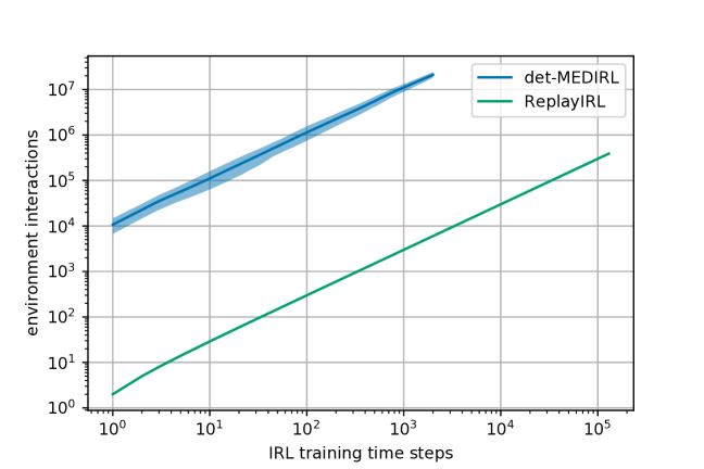
Figure 6: Environment interactions vs. training time step for IRL methods. Note the log-log axis implies a much faster growth rate for det-MEDIRL. Shaded region for det-MEDIRL represents variance among all seeds.

VII CONCLUSIONS

In this paper, we considered the important problem of robotic social navigation, which will play a crucial role in the integration of mobile robotics into previously human-inhabited social spaces. We presented ReplayIRL, an IRL approach to social navigation which we demonstrate is more sample efficient, more performant, and faster to train than alternative IRL based methods. In addition to this, future work might tackle methods of expert trajectory collection, feature extraction using commonly available robotic sensors, as well as improving the data efficiency of the algorithm.

References

- [1] C. Jayawardena, I. H. Kuo, U. Unger, A. Igic, R. Wong, C. I. Watson, R. Q. Stafford, E. Broadbent, P. Tiwari, J. Warren, J. Sohn, and B. A. MacDonald, “Deployment of a service robot to help older people,” in 2010 IEEE/RSJ International Conference on Intelligent Robots and Systems, Oct. 2010, pp. 5990–5995.
- [2] H.-M. Gross, H. Boehme, C. Schroeter, S. Mueller, A. Koenig, E. Einhorn, C. Martin, M. Merten, and A. Bley, “TOOMAS: Interactive Shopping Guide robots in everyday use - final implementation and experiences from long-term field trials,” in 2009 IEEE/RSJ International Conference on Intelligent Robots and Systems, Oct. 2009, pp. 2005–2012.
- [3] N. Mitsunaga, T. Miyashita, H. Ishiguro, K. Kogure, and N. Hagita, “Robovie-IV: A Communication Robot Interacting with People Daily in an Office,” in 2006 IEEE/RSJ International Conference on Intelligent Robots and Systems, Oct. 2006, pp. 5066–5072.
- [4] S. J. Guy, M. C. Lin, and D. Manocha, “Modeling collision avoidance behavior for virtual humans,” in Proceedings of the 9th International Conference on Autonomous Agents and Multiagent Systems: Volume 2 - Volume 2, ser. AAMAS ’10. Richland, SC: International Foundation for Autonomous Agents and Multiagent Systems, May 2010, pp. 575–582.
- [5] J. van den Berg, S. J. Guy, M. Lin, and D. Manocha, “Reciprocal n-Body Collision Avoidance,” in Robotics Research, ser. Springer Tracts in Advanced Robotics, C. Pradalier, R. Siegwart, and G. Hirzinger, Eds. Berlin, Heidelberg: Springer, 2011, pp. 3–19.
- [6] J. Müller, C. Stachniss, K. O. Arras, and W. Burgard, “Socially inspired motion planning for mobile robots in populated environments,” in Proc. of International Conference on Cognitive Systems, Karlsruhe, Germany, 2008.
- [7] P. E. Hart, N. J. Nilsson, and B. Raphael, “A Formal Basis for the Heuristic Determination of Minimum Cost Paths,” IEEE Transactions on Systems Science and Cybernetics, vol. 4, no. 2, pp. 100–107, July 1968.
- [8] M. Svenstrup, T. Bak, and H. J. Andersen, “Trajectory planning for robots in dynamic human environments,” in 2010 IEEE/RSJ International Conference on Intelligent Robots and Systems, Oct. 2010, pp. 4293–4298.
- [9] S. M. LaValle, “Rapidly-exploring random trees: A new tool for path planning,” Computer Science Department, Iowa State University, Technical Report 98-11, 1998.
- [10] D. Helbing and P. Molnar, “Social Force Model for Pedestrian Dynamics,” Physical Review E, vol. 51, May 1998.
- [11] D. Helbing and A. Johansson, “Pedestrian, Crowd and Evacuation Dynamics,” in Encyclopedia of Complexity and Systems Science, Apr. 2010, vol. 16, pp. 697–716.
- [12] A. Johansson, D. Helbing, and P. K. Shukla, “Specification of the Social Force Pedestrian Model by Evolutionary Adjustment to Video Tracking Data.” Advances in Complex Systems, vol. 10, pp. 271–288, Dec. 2007.
- [13] G. Ferrer, A. Garrell, and A. Sanfeliu, “Robot companion: A social-force based approach with human awareness-navigation in crowded environments,” in 2013 IEEE/RSJ International Conference on Intelligent Robots and Systems, Nov. 2013, pp. 1688–1694.
- [14] Y. F. Chen, M. Liu, M. Everett, and J. P. How, “Decentralized non-communicating multiagent collision avoidance with deep reinforcement learning,” in 2017 IEEE International Conference on Robotics and Automation (ICRA), May 2017, pp. 285–292.
- [15] M. Everett, Y. F. Chen, and J. P. How, “Motion Planning Among Dynamic, Decision-Making Agents with Deep Reinforcement Learning,” in 2018 IEEE/RSJ International Conference on Intelligent Robots and Systems (IROS), Oct. 2018, pp. 3052–3059.
- [16] S. Hochreiter and J. Schmidhuber, “Long Short-Term Memory,” Neural Computation, vol. 9, no. 8, pp. 1735–1780, Nov. 1997. [Online]. Available: https://doi.org/10.1162/neco.1997.9.8.1735
- [17] Y. F. Chen, M. Everett, M. Liu, and J. P. How, “Socially aware motion planning with deep reinforcement learning,” in 2017 IEEE/RSJ International Conference on Intelligent Robots and Systems (IROS), Sept. 2017, pp. 1343–1350.
- [18] B. D. Ziebart, A. L. Maas, J. A. Bagnell, and A. K. Dey, “Maximum entropy inverse reinforcement learning.” in Aaai, vol. 8, Chicago, IL, USA. Chicago, IL, USA, 2008, pp. 1433–1438.
- [19] K. M. Kitani, B. D. Ziebart, J. A. Bagnell, and M. Hebert, “Activity Forecasting,” in Computer Vision – ECCV 2012, ser. Lecture Notes in Computer Science, A. Fitzgibbon, S. Lazebnik, P. Perona, Y. Sato, and C. Schmid, Eds. Berlin, Heidelberg: Springer, 2012, pp. 201–214.
- [20] D. Vasquez, B. Okal, and K. O. Arras, “Inverse Reinforcement Learning algorithms and features for robot navigation in crowds: An experimental comparison,” in 2014 IEEE/RSJ International Conference on Intelligent Robots and Systems. Chicago, IL, USA: IEEE, Sept. 2014, pp. 1341–1346. [Online]. Available: http://ieeexplore.ieee.org/document/6942731/
- [21] P. Henry, C. Vollmer, B. Ferris, and D. Fox, “Learning to navigate through crowded environments,” in 2010 IEEE International Conference on Robotics and Automation. Anchorage, AK: IEEE, May 2010, pp. 981–986. [Online]. Available: http://ieeexplore.ieee.org/document/5509772/
- [22] H. Kretzschmar, M. Spies, C. Sprunk, and W. Burgard, “Socially compliant mobile robot navigation via inverse reinforcement learning,” The International Journal of Robotics Research, vol. 35, no. 11, pp. 1289–1307, Sept. 2016. [Online]. Available: http://journals.sagepub.com/doi/10.1177/0278364915619772
- [23] M. Kuderer, H. Kretzschmar, C. Sprunk, and W. Burgard, “Feature-Based Prediction of Trajectories for Socially Compliant Navigation,” in Robotics: Science and Systems VIII, vol. 08, July 2012. [Online]. Available: http://www.roboticsproceedings.org/rss08/p25.html
- [24] H. Kretzschmar, M. Kuderer, and W. Burgard, “Learning to predict trajectories of cooperatively navigating agents,” in 2014 IEEE International Conference on Robotics and Automation (ICRA). Hong Kong, China: IEEE, May 2014, pp. 4015–4020. [Online]. Available: http://ieeexplore.ieee.org/document/6907442/
- [25] S. Pellegrini, A. Ess, K. Schindler, and L. van Gool, “You’ll never walk alone: Modeling social behavior for multi-target tracking,” in 2009 IEEE 12th International Conference on Computer Vision. Kyoto: IEEE, Sept. 2009, pp. 261–268. [Online]. Available: http://ieeexplore.ieee.org/document/5459260/
- [26] D. Ramachandran and E. Amir, “Bayesian Inverse Reinforcement Learning.” in IJCAI, vol. 7, 2007, pp. 2586–2591.
- [27] B. Okal and K. O. Arras, “Learning socially normative robot navigation behaviors with Bayesian inverse reinforcement learning,” in 2016 IEEE International Conference on Robotics and Automation (ICRA), May 2016, pp. 2889–2895.
- [28] G. Neumann, M. Pfeiffer, and W. Maass, “Efficient Continuous-Time Reinforcement Learning with Adaptive State Graphs,” in Machine Learning: ECML 2007, ser. Lecture Notes in Computer Science, J. N. Kok, J. Koronacki, R. L. de Mantaras, S. Matwin, D. Mladenič, and A. Skowron, Eds. Berlin, Heidelberg: Springer, 2007, pp. 250–261.
- [29] B. Kim and J. Pineau, “Socially Adaptive Path Planning in Human Environments Using Inverse Reinforcement Learning,” Int J of Soc Robotics, vol. 8, no. 1, pp. 51–66, Jan. 2016. [Online]. Available: http://link.springer.com/10.1007/s12369-015-0310-2
- [30] M. Wulfmeier, P. Ondruska, and I. Posner, “Maximum Entropy Deep Inverse Reinforcement Learning,” CoRR, vol. abs/1507.04888, Mar. 2016. [Online]. Available: http://arxiv.org/abs/1507.04888
- [31] M. Fahad, Z. Chen, and Y. Guo, “Learning How Pedestrians Navigate: A Deep Inverse Reinforcement Learning Approach,” in 2018 IEEE/RSJ International Conference on Intelligent Robots and Systems (IROS), Oct. 2018, pp. 819–826.
- [32] A. Alahi, V. Ramanathan, and L. Fei-Fei, “Socially-Aware Large-Scale Crowd Forecasting,” in 2014 IEEE Conference on Computer Vision and Pattern Recognition, June 2014, pp. 2211–2218.
- [33] A. Konar, B. H. Baghi, and G. Dudek, “Learning Goal Conditioned Socially Compliant Navigation From Demonstration Using Risk-Based Features,” IEEE Robotics and Automation Letters, vol. 6, no. 2, pp. 651–658, Apr. 2021.
- [34] C. Yang, X. Ma, W. Huang, F. Sun, H. Liu, J. Huang, and C. Gan, “Imitation learning from observations by minimizing inverse dynamics disagreement,” in Advances in Neural Information Processing Systems, H. Wallach, H. Larochelle, A. Beygelzimer, F. dAlché-Buc, E. Fox, and R. Garnett, Eds., vol. 32. Curran Associates, Inc., 2019. [Online]. Available: https://proceedings.neurips.cc/paper/2019/file/ed3d2c21991e3bef5e069713af9fa6ca-Paper.pdf
- [35] B. D. Ziebart, J. A. Bagnell, and A. K. Dey, “Modeling interaction via the principle of maximum causal entropy,” in Proceedings of the 27th International Conference on International Conference on Machine Learning, ser. ICML’10. Madison, WI, USA: Omnipress, June 2010, pp. 1255–1262.
- [36] C. Finn, S. Levine, and P. Abbeel, “Guided Cost Learning: Deep Inverse Optimal Control via Policy Optimization,” in International Conference on Machine Learning. PMLR, June 2016, pp. 49–58. [Online]. Available: http://proceedings.mlr.press/v48/finn16.html
- [37] C. Finn, P. Christiano, P. Abbeel, and S. Levine, “A Connection between Generative Adversarial Networks, Inverse Reinforcement Learning, and Energy-Based Models,” CoRR, vol. abs/1611.03852, Nov. 2016. [Online]. Available: http://arxiv.org/abs/1611.03852
- [38] L.-J. Lin, “Self-improving reactive agents based on reinforcement learning, planning and teaching,” Mach Learn, vol. 8, no. 3, pp. 293–321, May 1992. [Online]. Available: https://doi.org/10.1007/BF00992699
- [39] T. Haarnoja, A. Zhou, P. Abbeel, and S. Levine, “Soft Actor-Critic: Off-Policy Maximum Entropy Deep Reinforcement Learning with a Stochastic Actor,” in International Conference on Machine Learning. PMLR, July 2018, pp. 1861–1870. [Online]. Available: http://proceedings.mlr.press/v80/haarnoja18b.html
- [40] T. Haarnoja, A. Zhou, K. Hartikainen, G. Tucker, S. Ha, J. Tan, V. Kumar, H. Zhu, A. Gupta, P. Abbeel, and S. Levine, “Soft Actor-Critic Algorithms and Applications,” arXiv:1812.05905 [cs, stat], Dec. 2018. [Online]. Available: http://arxiv.org/abs/1812.05905
- [41] I. Kostrikov, K. K. Agrawal, D. Dwibedi, S. Levine, and J. Tompson, “Discriminator-actor-critic: Addressing sample inefficiency and reward bias in adversarial imitation learning,” in International Conference on Learning Representations, 2019. [Online]. Available: https://openreview.net/forum?id=Hk4fpoA5Km
- [42] J. Fu, K. Luo, and S. Levine, “Learning Robust Rewards with Adversarial Inverse Reinforcement Learning,” arXiv:1710.11248 [cs], Oct. 2017. [Online]. Available: http://arxiv.org/abs/1710.11248
- [43] A. Lerner, Y. Chrysanthou, and D. Lischinski, “Crowds by Example,” Computer Graphics Forum, vol. 26, no. 3, pp. 655–664, 2007. [Online]. Available: https://onlinelibrary.wiley.com/doi/abs/10.1111/j.1467-8659.2007.01089.x
- [44] V. Nair and G. E. Hinton, “Rectified linear units improve restricted boltzmann machines,” in Proceedings of the 27th International Conference on International Conference on Machine Learning, ser. ICML’10. Madison, WI, USA: Omnipress, June 2010, pp. 807–814.
- [45] I. Loshchilov and F. Hutter, “Decoupled weight decay regularization,” in 7th International Conference on Learning Representations, ICLR 2019, New Orleans, LA, USA, May 6-9, 2019. OpenReview.net, 2019. [Online]. Available: https://openreview.net/forum?id=Bkg6RiCqY7
- [46] E. T. Hall, Handbook for Proxemic Research. Society for the Anthropology of Visual Communication, 1974.