Verifying Safe Transitions between Dynamic Motion Primitives on Legged Robots

Abstract

Functional autonomous systems often realize complex tasks by utilizing state machines comprised of discrete primitive behaviors and transitions between these behaviors. This architecture has been widely studied in the context of quasi-static and dynamics-independent systems. However, applications of this concept to dynamical systems are relatively sparse, despite extensive research on individual dynamic primitive behaviors, which we refer to as “motion primitives.” This paper formalizes a process to determine dynamic-state aware conditions for transitions between motion primitives in the context of safety. The result is framed as a “motion primitive graph” that can be traversed by standard graph search and planning algorithms to realize functional autonomy. To demonstrate this framework, dynamic motion primitives—including standing up, walking, and jumping—and the transitions between these behaviors are experimentally realized on a quadrupedal robot.

I INTRODUCTION

There is a significant volume of literature, applications, and demonstrations of functional autonomous systems that perform a wide range of complex tasks, ranging from the unstructured environment of disaster-response motivated DARPA Robotics Challenge [1] to the highly structured environment of industrial manufacturing robotics [2]. These systems often use sequence-based [3, 4], state-machine based [5], or graph-based [6] autonomy to couple many discrete behaviors together to complete highly complex tasks. These applications are typically quasi-static or have dynamics which are self-contained within each primitive behavior; thus, task-level or pose states can be used to determine if transitions are safe, while dynamic states are not considered. If one intends to extend this concept to dynamic systems and transitions, then the dynamic nature of the primitive behaviors and the transitions between them must be considered explicitly. This observation motivates the desire to determine safe transitions between what are referred to as “motion primitives” [7, 8, 9].

There is a wealth of prior work on motion primitives, examples of which include walking, running and jumping for legged robotics [10, 11], lane-following, cruise control and parallel parking for wheeled vehicles [12], and hovering and landing for quadrotor applications [13]. It is important to note that there exist many different methods to realize a given behavior, with varying advantages and disadvantages in the aspects of safety, performance, robustness to uncertainty, etc. Certain methods for generating motion primitives may be more or less conducive for use in our proposed framework. Rather than focus on specific approaches, the goal of this paper is to detail a general framework for studying motion primitives and transitions that is verifiable and, importantly, realizable on dynamic legged robotic systems.

Of special interest in this work are transitions between dynamic motion primitives. For these primitives, transitioning requires convergence to the next primitive while maintaining safety, and can be studied through the notions of stability and regions of attraction. There are a number of effective techniques to estimate regions of attraction, including backward reachability methods [14], optimization-based Lyapunov methods [15, 16, 17], quadratic Lyapunov methods [18] and linearization methods [19]. Additionally, Control Lyapunov Function and Control Barrier Function-based motion primitives [20] can also be used to enforce both stability and safety explicitly. In this paper, we leverage these ideas to verify safe transitions.

Figure 1: A depiction of the motion primitive graph and the Unitree A1 executing the graph dynamically.

The main result of this paper is a formalization of dynamic motion primitives and transition types between them, and a method to verify the availability of transitions between arbitrary primitives. This leads to the construction of a “motion primitive graph” that can be utilized via standard graph search algorithms to provide a certifiably-safe transition path between the execution of motion primitives; see Figure 1. This method was applied to a set of quadrupedal motion primitives and validated through hardware experiments on a Unitree A1 quadruped. The results demonstrate successful and safe execution of a complex sequence of desired dynamic behaviors, e.g., walking and jumping, and a comparison with naïve transitioning highlights the contributions of this work.

II Preliminaries

Consider a nonlinear system in control affine form:

$$\dot{x}=f(x)+g(x)u$$

where ${x\in\mathcal{X}\subset\mathbb{R}^{n}}$ is the state of the system, $u\in\mathcal{U}\subset\mathbb{R}^{m}$ represents the control inputs, and the functions ${f:\mathcal{X}\to\mathbb{R}^{n}}$ and ${g:\mathcal{X}\to\mathbb{R}^{n\times m}}$ are assumed to be locally Lipschitz continuous. Under the application of a locally Lipschitz continuous feedback control law ${u=k(x,t)}$, we get the closed loop dynamics:

$$\dot{x}=f_{\rm cl}(x,t)=f(x)+g(x)k(x,t).$$ (1)

For these dynamics, the solution to the initial value problem with ${x(0)=x_{0}}$ is termed the flow of the system and is denoted as $\phi_{t}(x_{0})$. The flow exists for all $t\geq 0$ if we further assume that $\mathcal{X}$ and $\mathcal{U}$ are compact.

In the following constructions, we describe the closed-loop behavior $\phi_{t}(x_{0})$ by the help of motion primitives. While motion primitives are not a novel concept [7, 8, 9], we introduce our own definition that facilitates the construction of motion primitive graphs for use in planning and autonomy.

Definition 1.

A motion primitive is a dynamic behavior of (1) defined by the 6-tuple $\mathcal{P}={(x^{*},k,\Omega,\mathcal{C},\mathcal{S},\mathcal{E})}$ with the following attributes.

• The setpoint, ${x^{*}:\mathbb{R}\to\mathcal{X}}$, that describes the desired state as a function of time by $x^{*}(t)$. It satisfies (1) and hence ${x^{*}(t+t_{0})=\phi_{t}(x^{*}(t_{0}))}$, ${\forall t\geq 0,t_{0}\in\mathbb{R}}$. It may be executed with a selected initial time $t_{0}$.

• The control law, ${k:\mathcal{X}\times\mathbb{R}\to\mathcal{U}}$, that determines the control input ${u=k(x,t)}$. It is assumed to render the setpoint locally asymptotically stable.

• The region of attraction (RoA) of the setpoint, ${\Omega:\mathbb{R}\to\mathcal{X}}$, given by ${\Omega(t_{0})\subseteq\mathcal{X}}$:

  $$\Omega(t_{0})=\{x_{0}\in\mathcal{X}:\lim_{t\to\infty}\phi_{t}(x_{0})\!-\!x^{*}(t\!+\!t_{0})=0\}.$$ (2)

• The safe set, ${\mathcal{C}:\mathbb{R}\to\mathcal{X}}$, that indicates the states of safe operation by the set ${\mathcal{C}(t)\subset\mathcal{X}}$. It is assumed to be the 0-superlevel set of a function ${h:\mathcal{X}\times\mathbb{R}\to\mathbb{R}}$:

  $$\mathcal{C}(t)=\{x\in\mathcal{X}:h(x,t)\geq 0\},$$

  such that ${x^{*}(t+t_{0})\in\mathcal{C}(t)}$, ${\forall t\geq 0,t_{0}\in\mathbb{R}}$.

• The implicit safe region of attraction, ${\mathcal{S}:\mathbb{R}\to\mathcal{X}}$, that defines the set of points from which the flow converges to the setpoint while being safe for all time:

  $$\mathcal{S}(t_{0})=\{x_{0}\in\Omega(t_{0}):\phi_{t}(x_{0})\in\mathcal{C}(t),\forall t\geq 0\}.$$ (3)

  This set is non-empty as ${x^{*}(t_{0})\in\mathcal{S}(t_{0})}$. In general, it is difficult to compute this set, thereby the term implicit.

• The explicit safe region of attraction, ${\mathcal{E}:\mathbb{R}\to\mathcal{X}}$. Because finding $\mathcal{S}(t_{0})$ is difficult, we consider a smaller, known subset ${\mathcal{E}(t_{0})\subseteq\mathcal{S}(t_{0})}$ with ${x^{*}(t_{0})\in\mathcal{E}(t_{0})}$, ${\forall t_{0}\in\mathbb{R}}$.

II-A Motion Primitive Classes

We consider three classes of motion primitives, fixed, periodic and transient, given by the examples below.

Example 1.

A fixed motion primitive is a behavior where the setpoint and safe RoA are constant in time: ${x^{*}(t)=x^{*}}$, ${\mathcal{S}(t)=\mathcal{S}}$, ${\forall t\geq 0}$. Examples in this class include stand and sit behaviors for a legged robots, hover in place for a multirotor, and hold position behavior for a robotic manipulator.

Example 2.

A periodic motion primitive is a behavior where the setpoint and safe RoA are periodic in time: ${x^{*}(t)=x^{*}(t+T_{\rm p})}$, ${\mathcal{S}(t)=\mathcal{S}(t+T_{\rm p})}$, with period ${T_{\rm p}>0}$. Examples of this class are walking or running for legged robotics and repeated motions for pick-and-place robotics.

Example 3.

A transient motion primitive is a behavior where the setpoint and safe RoA are functions of time on a finite domain: $x^{*}(t)$, $\mathcal{S}(t)$, ${t\in[t_{0},t_{\rm f}]}$. Jumping and landing behaviors on legged platforms and tracking path-planned trajectories are examples of transient motion primitives.

These motion primitive classes are summarized in Table I. For each class indicators will be used for visualization in motion primitive graphs: box denotes fixed, circle represents periodic and diamond indicates transient motion primitives.

TABLE I: Motion Primitive Classes

Name	Setpoint	Safe RoA	Indicator
Fixed	$x^{*}(t)=x^{*}$	$\mathcal{S}(t)=\mathcal{S}$
Periodic	$x^{*}(t)=x^{*}(t+T)$	$\mathcal{S}(t)=\mathcal{S}(t+T)$
Transient	$x^{*}(t),t\in[t_{0},t_{\rm f}]$	$\mathcal{S}(t),t\in[t_{0},t_{\rm f}]$

II-B Motion Primitive Transitions

Having defined motion primitives, we investigate the transitions between them. Let us consider motion primitives $A,B\in\mathcal{P}$, a time moment $t_{A}\in\mathbb{R}_{\geq 0}$, the setpoint $x_{A}^{*}$ of $A$ and the controller $k_{B}$ of $B$.

Definition 2.

The flow $\phi_{t}^{B}(x_{A}^{*}(t_{A}))$ under controller $k_{B}$ starting from $x_{A}^{*}(t_{A})$ is called a transition $\mathcal{T}_{AB}$ from $A$ to $B$ starting at time $t_{A}$, if ${\exists t_{B}\in\mathbb{R}\;\;\text{s.t.}\;\;x_{A}^{*}(t_{A})\in\mathcal{S}_{B}(t_{B})}$.

To achieve a transition from $A$ to $B$, the control law $k_{B}$ of primitive $B$ can be applied starting from $t_{A}$ by selecting the appropriate $t_{B}$. The transition is safe by construction, since the definition of $S_{B}$ implies ${\phi_{t}^{B}(x_{A}^{*}(t_{A}))\in\mathcal{C}(t)}$, ${\forall t\geq t_{A}}$. If $t_{B}$ exists for all ${t_{A}\geq 0}$, the transition can be initiated at anytime from primitive $A$. We call this case as Class 1 transition. Otherwise, transition can only be initiated at some specific times $t_{A}$, which is called Class 2 transition. Class 1 and Class 2 transitions will be represented by solid and dashed edges in the motion primitive graph, respectively. If a transition does not exist between two primitives, then the control law $k_{B}$ may not guarantee a safe transition and no edge will exist in the motion primitive graph. In what follows, we reduce the problem of transitioning safely to verifying the existence of Class 1 or 2 transitions and switching from the controller of primitive $A$ to that of $B$ at the right moment of time.

II-C Motion Primitive Graph

Information about motion primitives and transitions between them can be organized into motion primitive graphs.

Definition 3.

A motion primitive graph $\mathcal{G}$ is a directed graph whose nodes are fixed, periodic or transient motion primitives and edges are Class 1 or Class 2 transitions. The motion primitive graph consists of $N$ motion primitive nodes $\{\mathcal{P}_{1},\ldots,\mathcal{P}_{N}\}$ with transitions $\mathcal{T}_{ij}$ potentially connecting node $\mathcal{P}_{i}$ to node $\mathcal{P}_{j}$ for ${i,j\in\{1,\ldots,N\}}$.

(a) Original incomplete graph, no transition

(b) Periodic Step-in-Place intermediate primitive

(c) Transient Acceleration intermediate primitive

(d) Modification of existing Walk primitive

Figure 2: Examples for mending an incomplete graph between Stand and Walk motion primitives.

An example of a motion primitive graph can be seen in Figure 1. In general, there are no guarantees that a graph from an arbitrary set of primitives is connected, although it is a necessity for each primitive to be reachable. While ensuring a collection of motion primitives forms a connected graph is outside the scope of this paper, we posit this can be done by the modification of existing nodes or introduction of intermediate nodes. This is illustrated in Figure 2 with an example using Stand and Walk primitives for a legged robotic system. Initially, we have no transition between the Stand and Walk primitives, perhaps due to the violation of a no-slip safety constraint. Examples to make this graph connected include: the introduction of a periodic Step-in-Place primitive, the introduction of a transient Accelerate primitive, and modifying the Walk primitive to respect the no-slip safety constraint. While this is a significant topic in its own right, we will not investigate this further in this paper and we make the assumption the given nodes form a connected graph.

III Constructing the Motion Primitive Graph

We now turn to the major contribution of this paper: verifying the existence of safe transitions between motion primitives. For the subsequent analysis, consider prior primitive $A$ and posterior primitive $B$.

III-A Transitions via Safety Oracle

Clearly, the goal is to determine if a transition exists from $A$ to $B$ based on the condition ${x_{A}^{*}(t_{A})\in\mathcal{S}_{B}(t_{B})}$ in Definition 2. The setpoint $x_{A}^{*}(t)$ is known from the construction of motion primitive $A$, and if we have a formulation for the safe RoA $\mathcal{S}_{B}(t)$, the desired result follows. Note that the safe set $\mathcal{C}_{B}(t)$ is designer-prescribed and known, and the remaining component of $\mathcal{S}_{B}(t)$ is the region of attraction. Because determining the RoA explicitly is difficult, if not impossible, for general systems and primitives we require an alternative method to determine if a transition exists. We make two observations:

1. We do not necessarily need an explicit formulation for $\mathcal{S}_{B}(t)$ to determine if $x_{A}^{*}(t_{A})\in\mathcal{S}_{B}(t_{B})$.

2. There is at least one point we know is in $\mathcal{S}_{B}(t)$: $x_{B}^{*}(t)$.

From observation 2, we hypothesize that there exists a neighborhood $\mathcal{E}_{B}(t)$ of $x_{B}^{*}(t)$, called explicit safe region of attraction (see Definition 1), that is a subset of $\mathcal{S}_{B}(t)$ and is tractable to compute. This can be constructed based on the safe set and a conservative estimate of the RoA. For example, if the control law $k_{B}$ renders $x^{*}_{B}$ exponentially stable, the converse Lyapunov theorem can be used to estimate the RoA via a norm bound. The existence of the explicit safe RoA $\mathcal{E}_{B}(t)$ combined with observation 1 leads to the idea of the safety oracle.

Definition 4.

For motion primitive $\mathcal{P}$, a safety oracle with horizon ${T>0}$ is a map $\mathcal{O}:\mathcal{X}\times\mathbb{R}\rightarrow\{0,1\}$ defined by:

$$\mathcal{O}(x_{0},t_{0})=\begin{cases}1&\text{if }\phi_{t}(x_{0})\in\mathcal{C}(t),\quad\forall t\in[0,T],\\ &\quad\text{and }\phi_{T}(x_{0})\in\mathcal{E}(t_{0}+T),\\ 0&\text{otherwise}.\end{cases}$$

This definition reduces the verification of safe transitions to the evaluation of the safety oracle $\mathcal{O}$ as follows.

Theorem 1.

If ${\exists t_{B}\in\mathbb{R}}$ such that ${\mathcal{O}_{B}(x_{A}^{*}(t_{A}),t_{B})=1}$, then there exists a transition $\mathcal{T}_{AB}$ starting at $t_{A}$ from motion primitive A to motion primitive B.

Proof.

By definition, ${\mathcal{O}_{B}(x_{A}^{*}(t_{A}),t_{B})=1}$ implies

$$\begin{split}&\phi_{t}^{B}(x_{A}^{*}(t_{A}))\in\mathcal{C}_{B}(t),\quad\forall t\in[0,T],\\ &\phi_{T}^{B}(x_{A}^{*}(t_{A}))\in\mathcal{E}_{B}(t_{B}+T)\subseteq\mathcal{S}_{B}(t_{B}+T),\end{split}$$ (4)

where $\mathcal{E}_{B}$ is a subset of $\mathcal{S}_{B}$ by construction. By the definition (3) of $\mathcal{S}_{B}$, the second line of (4) implies

$$\phi_{t}^{B}(x_{A}^{*}(t_{A}))\in\mathcal{C}_{B}(t),\quad\forall t\geq T$$ (5)

and

$$\lim_{\theta\to\infty}\phi_{\theta}^{B}\big{(}\phi_{T}^{B}(x_{A}^{*}(t_{A}))\big{)}-x_{B}^{*}(\theta+T+t_{B})=0.$$

Since ${\phi_{\theta}^{B}\big{(}\phi_{T}^{B}(x_{A}^{*}(t_{A}))\big{)}=\phi_{\theta+T}^{B}(x_{A}^{*}(t_{A}))}$, a change of coordinates ${t=\theta+T}$ leads to form (2) and gives ${x_{A}^{*}(t_{A})\in\Omega_{B}(t_{B})}$. With the first line of (4) and (5), this leads to ${x_{A}^{*}(t_{A})\in\mathcal{S}_{B}(t_{B})}$, which proves the existence of transition $\mathcal{T}_{AB}$. $\blacksquare$

Theorem 1 provides a practical way of verifying the existence of transitions: one needs to evaluate ${\mathcal{O}_{B}(x_{A}^{*}(t_{A}),t_{B})}$ for various $t_{B}$ values. When evaluating $\mathcal{O}_{B}$, the flow $\phi_{t}(x_{A}^{*}(t_{A}))$ over ${t\in[0,T]}$ can be computed by numerical simulation of (1) which can be terminated if the flow enters $\mathcal{E}_{B}$. This is illustrated in Figure 3. While the method is computationally tractable for finite $T$, it is conservative in the sense that Theorem 1 involves a sufficient condition and ${\mathcal{O}_{B}(x_{A}^{*}(t_{A}),t_{B})=0}$ does not necessarily rule out the existence of a transition. However, this conservativeness becomes negligible if $T$ is large enough, since the flow from all points of $S_{B}$ eventually enter $\mathcal{E}_{B}$.

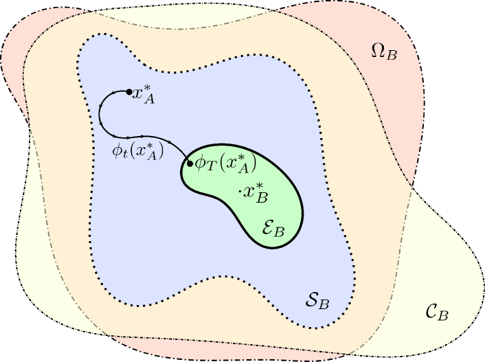
Figure 3: Illustration of the relationship of motion primitives $A$ and $B$ by the setpoints $x_{A}^{*}$ and $x_{B}^{*}$, flow $\phi_{t}(x_{A}^{*})$, region of attraction $\Omega_{B}$, safe set $\mathcal{C}_{B}$, implicit safe RoA $\mathcal{S}_{B}$, and explicit safe RoA $\mathcal{E}_{B}$.

III-B Constructing the Graph

Up until this point, we referred to motion primitives with distinct setpoints $x^{*}(t)$ and safe regions of attraction $\mathcal{S}(t)$. In practice, these may depend on certain parameters; dynamic behaviors may take a range of continuous or discrete arguments, such as walking speed or body orientation while standing in the case of legged robots. To support this with our framework, we quantize the argument space of behaviors, and treat each quanta as a unique motion primitive when constructing the motion primitive graph.

For each ordered pair of primitive, $A$ to $B$, we can then apply the safety oracle with respect to a discretization of time for primitive $A$. The flow in the safety oracle is computed via numerical integration of the system under $k_{B}$ for a parameterized time $T$. If the safety oracle returns True for all times in the discretization, we add a Class 1 transition to the graph from $A$ to $B$. If it returns True for only some times, we add a Class 2 transition to the graph. If the safety oracle never returns True, then no transition is added. Details can be found in Algorithm 1. It is important to note that this process can be done offline—in fact, this procedure only needs to be repeated if the dynamic model changes, existing primitives are modified, or new primitives are added. In the latter two cases, only a subset of motion primitive pairs needs to be rechecked for transitions. This results in a tractable procedure for constructing the motion primitive graph.

Algorithm 1 BuildMotionPrimitiveGraph

1:function BuildMotionPrimitiveGraph($\mathcal{P}$,T)

2:    $\mathcal{T}=\emptyset$$\triangleright$ $\mathcal{T}$ List of edges for motion primitive graph $\mathcal{G}$

3:    for $A,B\in\mathcal{P}$ do

4:         set $\mathcal{T}_{AB}=\emptyset$ $\triangleright$ Assume no transition exists

5:         set $SO{(\cdot,\cdot)}$ = False $\triangleright$ Safety Oracle responses

6:         for $(t_{A},t_{B})\in[t_{0A},t_{{\rm f}A}]\times[t_{0B},t_{{\rm f}B}]$ do

7:             set $SO{(t_{A},t_{B})}=$SafetyOracle$(f_{{\rm cl},B(t_{B})},x^{*}_{A},$ …                                $\mathcal{E}_{B}(t_{B}),\mathcal{C}_{B}(t_{B}),T)$

8:         end for

9:         if  any($SO{(\cdot,\cdot)}=$ True) then

10:             set $\mathcal{T}_{AB}=$ Class 2

11:         end if

12:         if $\forall\ t_{A}$ any($SO{(t_{A},\cdot)}$ = True) then

13:             set $\mathcal{T}_{AB}=$ Class 1

14:         end if

15:         AddEdge$(\mathcal{T},\mathcal{T}_{AB})$

16:    end for

17:    return $\mathcal{G}=(\mathcal{P},\mathcal{T})$

18:end function

19:

20:function SafetyOracle($f_{\rm cl},x^{*}$, $\mathcal{E},\mathcal{C},T$)

21:    $t=0$

22:    while $t<T$ do

23:         $\phi_{t}(x^{*})=$ Integrate($f_{\rm cl}(x^{*})$)

24:         if $\phi_{t}(x^{*})\in\mathcal{E}$ then

25:             return True

26:         end if

27:         if $\phi_{t}(x^{*})\notin\mathcal{C}$ then

28:             return False

29:         end if

30:    end while

31:    return False

32:end function

IV Application to Quadrupeds

The proposed concepts are applied to the Unitree A1 quadrupedal robot, shown in Figure 1, with a small set of motion primitives. In this setting, we define the local configuration space coordinates as $q\in\mathcal{Q}\subset\mathbb{R}^{n}$ with the full state space given by $x=(q,\dot{q})\in\mathcal{X}=T\mathcal{Q}\subset\mathbb{R}^{2n}$; in the case of the Unitree A1, $n=18$. The control input is given by $u\in\mathcal{U}\subset\mathbb{R}^{m}$, with $m=12$ actuators for the A1. During walking, the no slip condition of the feet is enforced via holonomic constraints, encoded by $c(q)\equiv 0$ for $c(q)\in\mathbb{R}^{n_{c}}$, where $n_{c}$ depends on the number of feet in contact with the ground. Differentiating $c(q)$ twice, D’Alembert’s principle applied to the constrained Euler-Lagrange equations gives:

$$D(q)\ddot{q}+H(q,\dot{q}) =Bu+J(q)^{\top}\lambda,$$

$$J(q)\ddot{q}+\dot{J}(q,\dot{q})\dot{q} =0,$$

where $D(q)\in\mathbb{R}^{n\times n}$ is the mass-inertia matrix, $H(q,\dot{q})\in\mathbb{R}^{n}$ contains the Coriolis and gravity terms, $B\in\mathbb{R}^{n\times m}$ is the actuation matrix, $J(q)=\partial c(q)/\partial q\in\mathbb{R}^{n_{c}\times n}$ is the Jacobian of the holonomic constraints, and $\lambda\in\mathbb{R}^{n_{c}}$ is the constraint wrench. This can be converted to control affine form:

$$\dot{x}=\underbrace{\begin{bmatrix}\dot{q}\\ -D(q)^{-1}(H(q,\dot{q})-J(q)^{\top}\lambda)\end{bmatrix}}_{f(x)}+\underbrace{\begin{bmatrix}0\\ D(q)^{-1}B\end{bmatrix}}_{g(x)}u,$$

where the mappings ${f:\mathcal{X}\to\mathbb{R}^{n}}$ and ${g:\mathcal{X}\to\mathbb{R}^{n\times m}}$ are assumed to be locally Lipschitz continuous. In the case of legged locomotion, the alternating sequences of continuous and discrete dynamics are captured within the hybrid dynamics framework. For the sake of simplicity, and because only the continuous dynamics are considered in the controller design process, this development will be omitted; please refer to [10] for more details. Finally, the outputs being driven to zero by the controllers in each respective motion primitive can be represented as:

$$y(x,t)=y^{\rm a}(x)-y^{\rm d}(t),$$

where the actual measured state $y^{\rm a}:\mathcal{X}\to\mathbb{R}^{o}$ and the desired state $y^{\rm d}:\mathbb{R}\to\mathbb{R}^{o}$ are smooth functions.

IV-A Quadruped Motion Primitives Preliminaries

Recall that our framework is agnostic to the implementation details of the primitives themselves, granted the assumptions in Section II are met. Nevertheless, the implementation details, along with the computable components of the motion primitive tuple, $(x^{*},k,\mathcal{C},\mathcal{E})\subset\mathcal{P}$, are elucidated for each primitive in our application. We begin by defining some common attributes.

Common Safe Sets.

For all primitives, the safety functions employed on hardware include joint position and velocity limits, whereby a combined safe set can be constructed as:

$$\mathcal{C}_{q,\dot{q}}=\{x\in\mathcal{X}:\; h_{q_{\rm min}}(x)=q-q_{\rm min}\geq 0,$$

$$h_{q_{\rm max}}(x)=q_{\rm max}-q\geq 0,$$

$$h_{\dot{q}_{\rm min}}(x)=\dot{q}-\dot{q}_{\rm min}\geq 0,$$

$$h_{\dot{q}_{\rm max}}(x)=\dot{q}_{\rm max}-\dot{q}\geq 0\}.$$

Additionally, many primitives require immobile ground contact with all feet for safety. Assuming a flat ground at $z=0$, this can be captured by safety functions:

$$\mathcal{C}_{\rm ground}=\{x\in\mathcal{C}_{q,\dot{q}}:\; h_{{\rm g}1}(x)=-fk_{z}(q)\geq 0,$$

$$h_{{\rm g}2}(x)=-J(q)\dot{q}=0\},$$

where $fk_{z}:\mathcal{Q}\to\mathbb{R}^{4}$ is the $z$-component of the forward kinematics of the feet of the quadruped.

Common Explicit Safe Regions of Attraction.

As discussed in Section III-A, we can choose a conservative safe RoA estimate $\mathcal{E}$ and compensate with an increased integration horizon T. For all the primitives in the experiment, we take a conservative norm bound about $x^{*}(t)$:

$$\mathcal{E}(t)=\{x\in\mathcal{X}:||x-x^{*}(t)||<r\},$$

where the value of $r$ is determined empirically for each primitive.

Motion Profiling.

Where indicated, motion primitives utilize cubic polynomial motion profiling over a fixed duration ${\Theta>0}$. This is computed via linear matrix equation:

$$\begin{bmatrix}c_{0}\\ c_{1}\\ c_{2}\\ c_{3}\end{bmatrix}=\begin{bmatrix}1&0&0&0\\ 1&\Theta&\Theta^{2}&\Theta^{3}\\ 0&1&0&0\\ 0&1&2\Theta^{2}&3\Theta^{2}\\ \end{bmatrix}^{-1}\begin{bmatrix}q_{0}\\ q_{\rm f}\\ \dot{q}_{0}\\ \dot{q}_{\rm f}\end{bmatrix},$$

where ${x_{A}^{*}=(q_{0},\dot{q}_{0})}$ and ${x^{*}_{B}=(q_{\rm f},\dot{q}_{\rm f})}$. Taking the desired state as ${y^{\rm d}(t)=(q^{\rm d}(t),\dot{q}^{\rm d}(t))}$, we have the polynomial:

$$y^{\rm d}(t) =\begin{cases}(q_{0},\dot{q}_{0})&\text{if }t<0,\\ \begin{matrix}(c_{0}+c_{1}t+c_{2}t^{2}+c_{3}t^{3},\\ c_{1}+2c_{2}t+3c_{3}t^{)}\end{matrix}&\text{if }t\in[0,\Theta],\\ (q_{\rm f},\dot{q}_{\rm f})&\text{if }t>\Theta.\\ \end{cases}$$ (6)

IV-B Quadruped Motion Primitives

We considered the motion primitives listed below:

Lie.

The Lie is a fixed motion primitive that rests the quadruped on the ground with the legs in a prescribed position. The feedback controller is a joint-space PD controller:

$$k(x,t)=-K_{P}y(x,t)-K_{D}\dot{y}(x,t),$$ (7)

where $y^{\rm d}(x,t)$ is the previously explained cubic spline in (6) from the pose when the primitive is first applied to the Lie goal pose, $x^{*}_{\rm Lie}$. The safe set for Lie requires ground contact from all four feet: $\mathcal{C}_{\rm Lie}=\mathcal{C}_{\rm ground}$.

Stand.

For the Stand fixed motion primitive, $x^{*}_{\rm Stand}$ prescribes the body to be at a specified height above the ground and the center of mass to lie above the centroid of the support polygon. Taking $\mathcal{X}_{\rm ext}=[\ddot{q}^{\top},u^{\top},\lambda^{\top}]^{\top}\in\mathbb{X}_{\rm ext}=\mathbb{R}^{18}\times\mathbb{R}^{12}\times\mathbb{R}^{n_{c}}$, this is done via an Inverse-Dynamics Quadratic Program based controller (ID-QP): ID-QP:

$${\mathcal{X}_{\rm ext}}^{*}=\underset{\mathcal{X}_{\rm ext}\in\mathbb{X}_{\rm ext}}{\mathrm{argmin}} \hskip 8.53581pt\|J_{y}(q,\dot{q})\ddot{q}+\dot{J}_{y}(q,\dot{q})\dot{q}-\tau(x,t)\|^{2}+\sigma W(\mathcal{X})$$

$$\mathrm{s.t.} \hskip 8.53581ptD(q)\ddot{q}+H(q,\dot{q})=Bu+J(q)^{\top}\lambda$$

$$\hskip 8.53581ptJ(q)\ddot{q}+\dot{J}(q,\dot{q})\dot{q}=0$$

$$\hskip 8.53581ptu\in\mathcal{U}$$

$$\hskip 8.53581pt\lambda\in\mathcal{FC}(x)$$

where $\mathcal{U}=[-33.5,33.5]^{12}$ is limited by the available torque at each motor, $\sigma$ and $\mathcal{W}$ are regularization terms for numerical stability of the QP, and $\mathcal{FC}(x)\in\mathbb{R}^{n_{c}}$ is a friction cone condition to enforce no slipping of the feet. The motion profile (6) in center of mass task-space is used with a PD control law to produce $\tau(x,t)$ in the objective function:

$$\tau(x,t)=K_{P}y(x,t)+K_{D}\dot{y}(x,t).$$

Finally, $k(x,t)=u^{*}$. We have the safe set: $\mathcal{C}_{\rm Stand}=\mathcal{C}_{\rm ground}.$

Walk.

The Walk periodic motion primitive locomotes the quadruped forward by tracking a stable walking gait. Stable walking gaits were generated using a biped-decomposition technique as described in [21] and combined in a gait library, [22]. Specifically, the desired output is written as:

$$x^{*}(t)=(x^{*}_{B}(t),\mathcal{R}x^{*}_{B}(t)),$$

where $x^{*}_{B}(t)$ is the desired behavior generated by the NLP toolbox FROST [23] for one biped, and ${\mathcal{R}\in\mathbb{R}^{o\times o}}$ is a mirroring matrix relating the behavior of the two subsystems. The gaits are tracked using the joint-space PD control law in (7). This primitive can be called with an argument to control forward speed, specifically: Walk(in place), Walk(slow), Walk(medium) and Walk(fast). Any slipping of stance feet is deemed unsafe, which is described by the safety function:

$$h_{i}(x)=\begin{cases}-J^{i}_{xy}(q)\dot{q}&\text{if }fk^{i}_{z}(q)\leq 0,\\ 0&\text{otherwise},\end{cases}$$

$$\mathcal{C}_{\rm Walk}=\{x\in\mathcal{C}_{q,\dot{q}}:\;h_{i}(x)=0,i\in\mathcal{F} \},$$

where $fk^{i}_{z}(q):\mathcal{Q}\to\mathbb{R}$ is the forward kinematics $z$-component, $J^{i}_{xy}(q):\mathcal{Q}\to\mathbb{R}^{2\times n}$ is the $x,y$-components of the Jacobian for each foot, and $\mathcal{F}\subset\{1,...,4\}$ is an index set of feet in ground contact.

Figure 4: Computed motion primitive graph for the experimental set of quadruped motion primitives.

Jump.

The transient Jump primitive is a four-legged vertical jump, performed by task-space tracking of $x^{*}_{\rm Jump}$, a prescribed center of mass trajectory to reach a specified takeoff velocity. The trajectory is generated via (6) and does not take constraints (input or otherwise) into account. The trajectory is tracked via a task-space PD control law:

$$k(x,t)=J_{y}(x)^{\top}\big{(}-K_{P}y(x,t)-K_{D}\dot{y}(x,t)\big{)},$$

where $J_{y}:\mathcal{X}\to\mathbb{R}^{o\times m}$ is the Jacobian of the outputs. Like other transient primitives, this requires a “next primitive” argument. For the purpose of this experiment, the next primitive will always be Land. To be in the safe set, the Jump primitive requires all feet to be in contact at ${t=0}$, and no feet to be in contact after prescribed takeoff time. For the aerial phase, we define:

$$\mathcal{C}_{\rm aerial}=\{x\in\mathcal{C}_{q,\dot{q}}:\; h(x)=fk_{z}(q)\geq 0\}.$$

The composite safe set is then:

$$\mathcal{C}_{\rm Jump}(t) =\begin{cases}\mathcal{C}_{\rm ground}&\text{if }t<T_{\rm t},\\ \mathcal{C}_{q,\dot{q}}&\text{if }T_{\rm t}\leq t<T_{\rm t}+\epsilon,\\ \mathcal{C}_{\rm aerial}&\text{if }T_{\rm t}+\epsilon\leq t<T_{\rm f},\\ \end{cases}$$

where $T_{\rm t}$ and $T_{\rm f}$ are the takeoff time and final time prescribed by the trajectory, and ${\epsilon>0}$ allows for non-simultaneous contact in the safe set.

Land.

The Land primitive is a high-damping joint-space PD control law, as in (7), about a crouched pose, $x^{*}_{\rm Land}$, to cushion the quad as the legs make contact with the ground from an airborne state. In this experiment, the next primitive will always be Stand. The safe set for Land requires all feet to not be in contact at $t=0$ and all feet to reach contact within a small time window after initial ground contact:

$$\mathcal{C}_{\rm Land}(t) =\begin{cases}\mathcal{C}_{\rm aerial}&\text{if }t<T_{\rm c},\\ \mathcal{C}_{q,\dot{q}}&\text{if }T_{\rm c}\leq t<T_{\rm c}+\epsilon,\\ \mathcal{C}_{\rm ground}&\text{if }T_{\rm c}+\epsilon\leq t,\\ \end{cases}$$

where $T_{\rm c}$ is the time of first ground contact.

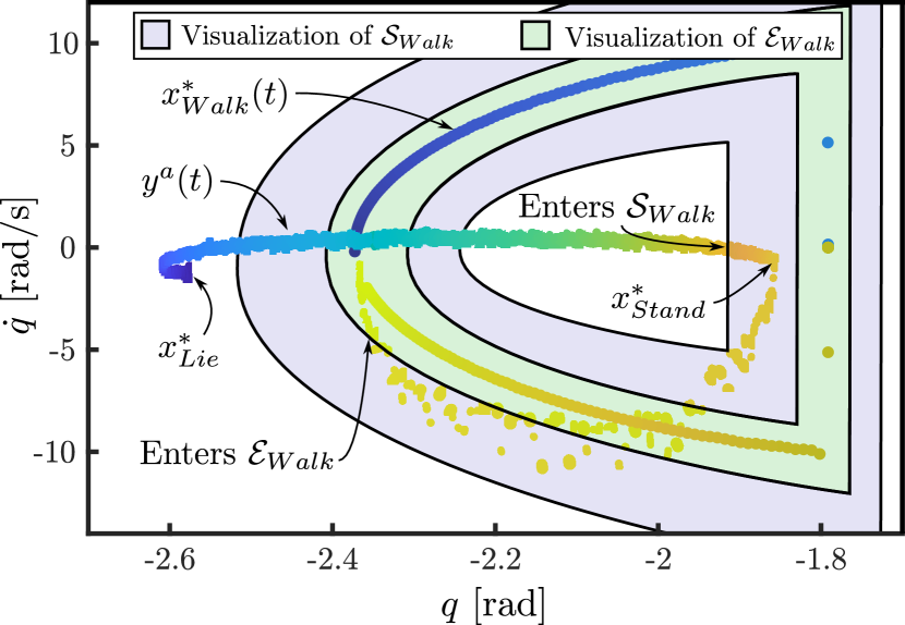
Figure 5: Depiction of the transition from Lie to Stand to Walk(in place) during the hardware experiments. The inclusion of $x^{*}_{\rm Stand}$ in the approximate $\mathcal{S}_{\rm Walk}$ can be seen, and upon switching to the controller for the walk primitive, the flow of the system eventually reaches $\mathcal{E}_{\rm Walk}$.

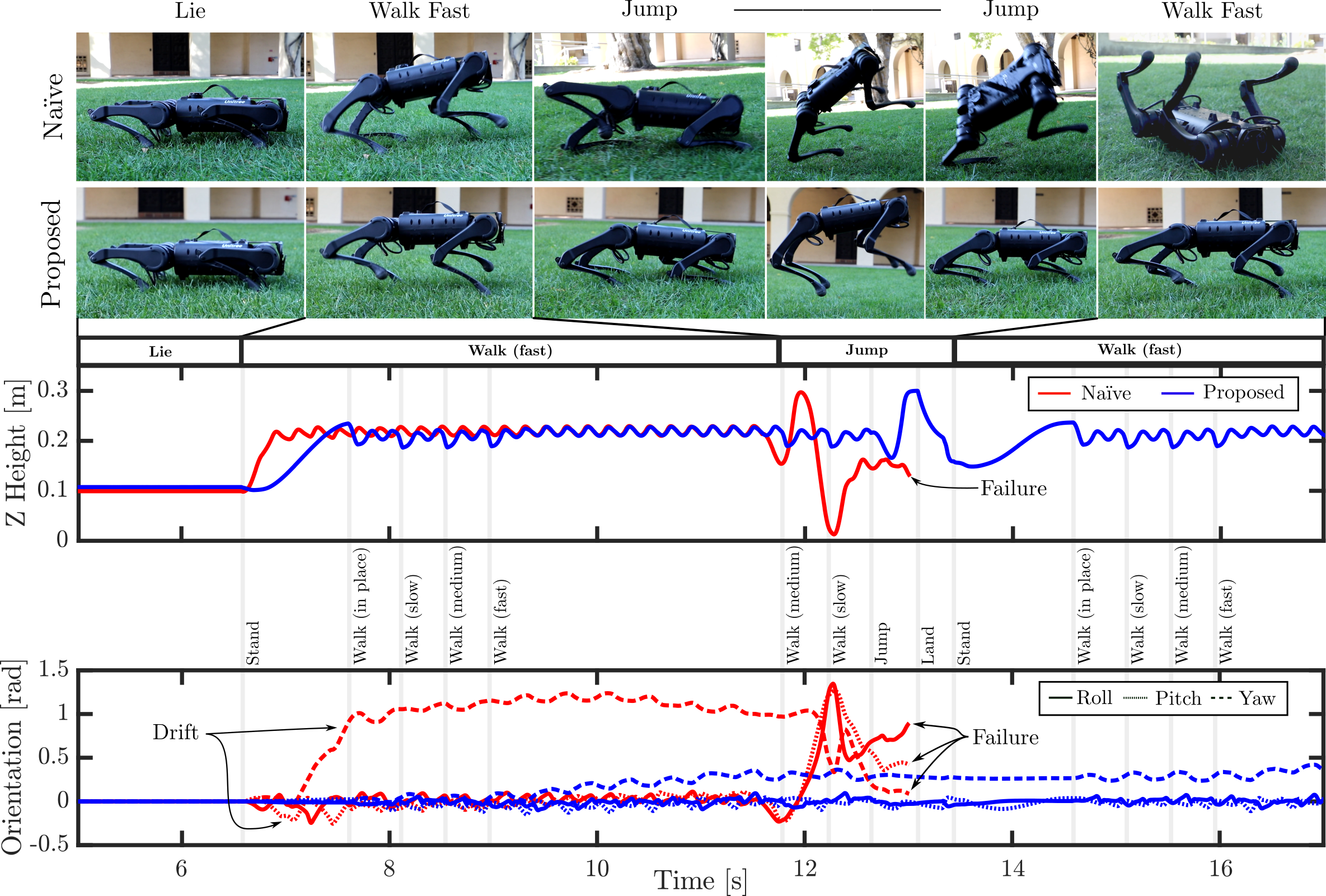
Figure 6: Motion primitive graph traversal for a sample sequence of desired primitives on quadrupedal system. Top: Gait tiles comparing the proposed method to a naïve method, which results in a violation of safety. Bottom: center of mass height and orientation comparison between naïve transitions and the proposed graph-traversal transitions. Blocks under the upper plot show desired behavior and vertical lines with corresponding text indicate the mode used by the proposed method. Note the substantial drift and ultimate failure when using the naïve transitions.

IV-C Implementation and Experimental Results

Each individual primitive was implemented as a C++ module with function calls for the computable portions of the motion primitive tuple, $(x^{*},k,\mathcal{C},\mathcal{E})\subset\mathcal{P}$. A C++ implementation of Algorithm 1 was applied, utilizing the Pinocchio Rigid Body dynamics library [24] and Boost’s odeint with a runge_kutta_cash_karp54 integration scheme [25]. Note that in the construction of the motion primitive graph, the hybrid nature of the system was taken into account.

The resulting motion primitive graph is visualized in Figure 4. The graph shows that we can freely transition from Lie to Stand, but must go through Walk(in place) before reaching other walk speeds. Additionally, the Class 2 transitions from the Walk states indicates the time-dependent nature of the transition: we can only leave the Walk primitive at certain times in the orbit.

TABLE II: Test Sequence of Goal Motion Primitives

Time	0 s	3 s	8 s	11 s	16 s
Goal Primitive	Lie	Walk(fast)	Jump	Walk(fast)	Lie
Inter. Primitives	—	Lie Stand Walk(in place) Walk(slow) Walk(medium) Walk(fast)	Walk(fast) Walk(medium) Walk(slow) Walk(in place) Stand Jump	Jump Land Stand Walk(in place) Walk(slow) Walk(medium) Walk(fast)	Walk(fast) Walk(medium) Walk(slow) Walk(in place) Lie

Using the motion primitive graph, offline depth-first search was used to compute the path from each known current primitive to a desired motion primitive. The solutions were implemented as an online lookup table.

To validate the method experimentally, a sequence of goal primitives was built to exercise the different transition types in the quadruped example. The sequence is shown in Table II. Each desired primitive in the sequence was commanded at the listed time. Two cases were run with the sequence: the first with naïve, immediate application of the goal motion primitive, and the second with our proposed traversal algorithm executing intermediate motion primitives based on the motion primitive graph.

With the proposed traversal algorithm executing intermediate primitives, we see the transition from Lie to Walk(fast) first traverses through Stand, then Walk(in place) and other walk speeds until finally reaching Walk(fast) without violating the no-slip and other safety constraints. The evolution of the hardware system with respect to the desired behavior as well as a representation of the implicit and explicit safe sets can be seen in Figure 5. Likewise, when Jump is commanded, the current motion primitive traverses downward through the walk speeds and then to Stand before executing the vertical jump. As Jump is a transient primitive, this is followed by the Land and Stand primitives before traversing back to Walk(fast). The sequence ends successfully by cycling back down through the walk speeds to Walk(in place) before finishing at Lie. Unlike the naïve transitions, the graph traversal successfully and safely completes the sequence of desired motion primitives.

In the naïve case, the no-slip safety constraint is violated in the Lie to Walk(fast) transition. Furthermore, the Walk(fast) to Jump transition results in the failure of the Jump primitive to track the desired behavior, as the Walk(fast) dynamic state at the transition time is not in the region of attraction of the Jump primitive. These results can be inferred from the motion primitive graph, as there is no verification of a direct transition between Lie and Walk(fast) and Walk(fast) and Jump. Ultimately, the direct transitions fail to maintain safety and cannot perform the desired sequence of behaviors.

A video comparison between the naïve transitions and the graph-traversal transitions is provided as an attachment (see [26]) and a snapshot comparison of gait tiles and collected data can be seen in Figure 6.

V CONCLUSIONS

Motivated by the complex autonomy realized in the quasi-static robotics realm and heuristically on dynamic legged robots, this paper has leveraged ideas from dynamic systems to make the first steps toward formulating a theory of transition classes between “motion primitives”. With these fundamentals, we proposed a tractable procedure to verify the existence of transitions between motion primitives through the use of a safety oracle and subsequently presented an algorithm for the construction of a “motion primitive graph.” This graph is used to determine transition paths via standard graph search algorithms. To illustrate the viability of the method, it was applied to a quadrupedal robot and a set of quadrupedal motion primitives. This culminated in a demonstration of the capability of our method via experiments on hardware while the robot performed dynamic behaviors.

There are a number of extensions that we intend to investigate in future. We would like to expand the theory described in Section III to address real-world uncertainty and disturbances, and explore necessary conditions for $\phi_{T}(x_{A}^{*}(t))$ to enter $\mathcal{E}_{B}(t)$ in this context. In systems with a large number of motion primitives, the final graph may offer many paths from one primitive to another. We would like to consider a “weighted” motion primitive graph, and understand what metrics are useful as weights for transitions or primitive executions (e.g. transition duration, peak torque, etc.). Additionally, we recognize that this method only addresses the nominal use case of autonomy in dynamic systems, and does not offer a solution to arbitrary initial dynamic states or disturbances that throw the state outside the safe region of attraction of the currently active primitive. Future work intends to explore these open questions in the context of primitive behaviors and the motion primitive graph.

References

- [1] “DARPA robotics challenge,” https://www.darpa.mil/program/darpa-robotics-challenge, accessed: 2021-02-28.
- [2] M. R. Pedersen, L. Nalpantidis, R. S. Andersen, C. Schou, S. Bøgh, V. Krüger, and O. Madsen, “Robot skills for manufacturing: From concept to industrial deployment,” Robotics and Computer-Integrated Manufacturing, vol. 37, pp. 282–291, 2016.
- [3] S. Karumanchi et al., “Team robosimian: Semi-autonomous mobile manipulation at the 2015 DARPA robotics challenge finals,” Journal of Field Robotics, vol. 34, pp. 305–332, 3 2017.
- [4] K. Edelberg et al., “Software system for the Mars 2020 mission sampling and caching testbeds,” in 2018 IEEE Aerospace Conference, 2018, pp. 1–11.
- [5] T. Merz, P. Rudol, and M. Wzorek, “Control system framework for autonomous robots based on extended state machines,” in International Conference on Autonomic and Autonomous Systems (ICAS’06), 2006, pp. 14–14.
- [6] P. Kim, B. C. Williams, and M. Abramson, “Executing reactive, model-based programs through graph-based temporal planning,” in IJCAI. Citeseer, 2001, pp. 487–493.
- [7] H. Zhao, M. J. Powell, and A. D. Ames, “Human-inspired motion primitives and transitions for bipedal robotic locomotion in diverse terrain,” Optimal Control Applications and Methods, vol. 35, pp. 730–755, 11 2014.
- [8] A. A. Paranjape, K. C. Meier, X. Shi, S.-J. Chung, and S. Hutchinson, “Motion primitives and 3D path planning for fast flight through a forest,” The International Journal of Robotics Research, vol. 34, no. 3, pp. 357–377, 2015.
- [9] A. Singla, S. Bhattacharya, D. Dholakiya, S. Bhatnagar, A. Ghosal, B. Amrutur, and S. Kolathaya, “Realizing learned quadruped locomotion behaviors through kinematic motion primitives,” in 2019 International Conference on Robotics and Automation (ICRA), 2019, pp. 7434–7440.
- [10] E. R. Westervelt, J. W. Grizzle, C. Chevallereau, J. H. Choi, and B. Morris, Feedback control of dynamic bipedal robot locomotion. CRC press, 2018.
- [11] D. Kim, J. Di Carlo, B. Katz, G. Bledt, and S. Kim, “Highly dynamic quadruped locomotion via whole-body impulse control and model predictive control,” arXiv preprint arXiv:1909.06586, 2019.
- [12] F. Gómez-Bravo, F. Cuesta, and A. Ollero, “Parallel and diagonal parking in nonholonomic autonomous vehicles,” Engineering Applications of Artificial Intelligence, vol. 14, no. 4, pp. 419–434, 2001.
- [13] D. Falanga, A. Zanchettin, A. Simovic, J. Delmerico, and D. Scaramuzza, “Vision-based autonomous quadrotor landing on a moving platform,” in 2017 IEEE International Symposium on Safety, Security and Rescue Robotics (SSRR). IEEE, 2017, pp. 200–207.
- [14] G. Yuan and Y. Li, “Estimation of the regions of attraction for autonomous nonlinear systems,” Transactions of the Institute of Measurement and Control, vol. 41, no. 1, pp. 97–106, 2019.
- [15] L. G. Matallana, A. M. Blanco, and J. A. Bandoni, “Estimation of domains of attraction: A global optimization approach,” Mathematical and Computer Modelling, vol. 52, no. 3, pp. 574–585, 2010.
- [16] T. A. Johansen, “Computation of Lyapunov functions for smooth nonlinear systems using convex optimization,” Automatica, vol. 36, no. 11, pp. 1617–1626, 2000.
- [17] A. Polanski, “Lyapunov function construction by linear programming,” IEEE Transactions on Automatic Control, vol. 42, no. 7, pp. 1013–1016, 1997.
- [18] E. Davison and E. Kurak, “A computational method for determining quadratic Lyapunov functions for non-linear systems,” Automatica, vol. 7, no. 5, pp. 627–636, 1971.
- [19] H. K. Khalil, “Nonlinear systems,” 2002.
- [20] A. D. Ames, X. Xu, J. W. Grizzle, and P. Tabuada, “Control barrier function based quadratic programs for safety critical systems,” IEEE Transactions on Automatic Control, vol. 62, no. 8, pp. 3861–3876, 2016.
- [21] W.-L. Ma, N. Csomay-Shanklin, and A. D. Ames, “Coupled control systems: Periodic orbit generation with application to quadrupedal locomotion,” IEEE Control Systems Letters, vol. 5, no. 3, pp. 935–940, 2021.
- [22] J. Reher and A. D. Ames, “Inverse dynamics control of compliant hybrid zero dynamic walking,” 2020. [Online]. Available: http://ames.caltech.edu/reher2020inversewalk.pdf
- [23] A. Hereid and A. D. Ames, “FROST: Fast robot optimization and simulation toolkit,” in 2017 IEEE/RSJ International Conference on Intelligent Robots and Systems (IROS). IEEE, 2017, pp. 719–726.
- [24] J. Carpentier, F. Valenza, N. Mansard, et al., “Pinocchio: fast forward and inverse dynamics for poly-articulated systems,” https://stack-of-tasks.github.io/pinocchio, 2015–2021.
- [25] Boost, “Boost C++ Libraries,” http://www.boost.org/, 2021, last accessed 2021-02-28.
- [26] Supplementary video, https://youtu.be/3vsk00a4XBg.