Efficient Computation of $N$-Point Correlation Functions in $D$ Dimensions

Abstract

We present efficient algorithms for computing the $N$-point correlation functions (NPCFs) of random fields in arbitrary $D$-dimensional homogeneous and isotropic spaces. Such statistics appear throughout the physical sciences, and provide a natural tool to describe stochastic processes. Typically, algorithms for computing the NPCF components have $\mathcal{O}(n^{N})$ complexity (for a data set containing $n$ particles); their application is thus computationally infeasible unless $N$ is small. By projecting the statistic onto a suitably-defined angular basis, we show that the estimators can be written in a separable form, with complexity $\mathcal{O}(n^{2})$, or $\mathcal{O}(n_{\rm g}\log n_{\rm g})$ if evaluated using a Fast Fourier Transform on a grid of size $n_{\rm g}$. Our decomposition is built upon the $D$-dimensional hyperspherical harmonics; these form a complete basis on the $(D-1)$-sphere and are intrinsically related to angular momentum operators. Concatenation of $(N-1)$ such harmonics gives states of definite combined angular momentum, forming a natural separable basis for the NPCF. As $N$ and $D$ grow, the number of basis components quickly becomes large, providing a practical limitation to this (and all other) approaches: however, the dimensionality is greatly reduced in the presence of symmetries; for example, isotropic correlation functions require only states of zero combined angular momentum. We provide a Julia package implementing our estimators, and show how they can be applied to a variety of scenarios within cosmology and fluid dynamics. The efficiency of such estimators will allow higher-order correlators to become a standard tool in the analysis of random fields.

This manuscript was compiled on

Random fields are ubiquitous in the physical sciences. Perhaps the most powerful tool for their analysis is the set of $N$-point correlation functions (hereafter NPCFs), defined as statistical averages over $N$ copies of the field at different spatial or temporal locations. If the field is Gaussian-random, only the first two correlators (the mean and two-point function) contain useful information, though this assumption is rarely true in practice. Examples of higher-order NPCFs populate many fields of study; a brief search will reveal their use in molecular physics (1), materials science (2), field theory (3), diffusive systems (4, 5) and cosmology (6), amongst other topics.

Correlation functions have found extensive use in the analysis of spectroscopic galaxy surveys (e.g., 7). Whilst the majority of information is contained within the 2PCF, inclusion of the higher-order functions is expected to significantly tighten constraints on cosmological parameters, particularly those pertaining to phenomena such as extensions to General Relativity (8). Despite this, statistics beyond the 2PCF have been scarcely used in practice; in fact, almost no modern analyses have included correlators with $N>3$. The reason is simple: higher-order NPCFs are expensive to compute and analyze.

Consider a $D$-dimensional space $\mathbb{M}^{D}$ (e.g., a Euclidean space) with an associated complex-valued random field $X:\mathbb{M}^{D}\to\mathbb{C}$. The NPCF, $\zeta:\left(\mathbb{M}^{D}\right)^{\otimes(N-1)}\to\mathbb{C}$ (for tensor product $\otimes$), is formally defined as

$$\boxed{\zeta(\mathbf{r}^{1},\ldots,\mathbf{r}^{N-1};\mathbf{s})=\mathbb{E}_{X}\left[X(\mathbf{s})X(\mathbf{s}+\mathbf{r}^{1})\cdots X(\mathbf{s}+\mathbf{r}^{N-1})\right],}$$ (1)

where $\mathbb{E}_{X}$ represents the statistical average over realizations of $X$, $\mathbf{s}$ and $\mathbf{r}^{i}$ are absolute and relative positions on the manifold, and we have assumed $N\geq 2$. If the random field is statistically homogeneous, all correlators must be independent of the absolute position $\mathbf{s}$; this leads to the well-known NPCF estimator

$$\boxed{\hat{\zeta}(\mathbf{r}^{1},\ldots,\mathbf{r}^{N-1})=\frac{1}{V_{D}}\int_{\mathbb{M}^{D}}d^{N}\mathbf{s}\,\left[X(\mathbf{s})X(\mathbf{s}+\mathbf{r}^{1})\cdots X(\mathbf{s}+\mathbf{r}^{N-1})\right],}$$ (2)

averaging $\mathbf{s}$ over a volume $V_{D}$, and noting that the NPCF depends on only $(N-1)$ positions. In praxis, we cannot estimate the continuous NPCF of (1); rather, we consider only the quantity projected onto some basis functions, $B(\mathbf{r}^{1},\ldots,\mathbf{r}^{N-1})$, for example a set of radial and angular bins. In this case, the problem reduces to estimating the coefficients $\zeta_{B}\equiv\int d\mathbf{r}^{1}\cdots d\mathbf{r}^{N-1}\zeta(\mathbf{r}^{1},\ldots,\mathbf{r}^{N-1})B(\mathbf{r}^{1},\ldots,\mathbf{r}^{N-1})$. Strictly, an infinite set of basis functions is required to fully specify the NPCF: conventionally, one restricts to a finite number, and applies the same basis projection to both data and theory, eliminating bias.

The computational difficulties become clear if one considers measuring the NPCF components from a discrete field containing $n$ particles. In this instance, the random field $X$ can be represented as a sum over $n$ Dirac delta functions, i.e. $X(\mathbf{r})=\sum_{j=1}^{n}w^{j}\delta^{\rm D}(\mathbf{r}-\mathbf{y}^{j})$, where $\{\mathbf{y}^{j}\}$ are the particle positions and $\{w^{j}\}$ are weights. Projecting onto a basis function $B$, the discrete version of (2) becomes

$$\hat{\zeta}_{B}=\frac{1}{V_{D}}\sum_{j_{0}=1}^{n}w^{j_{0}}\sum_{j_{1}=1}^{n}w^{j_{1}}\cdots\sum_{j_{N-1}=1}^{n}w^{j_{N-1}}B(\mathbf{y}^{j_{1}}-\mathbf{y}^{j_{0}},\ldots,\mathbf{y}^{j_{N-1}}-\mathbf{y}^{j_{0}}).$$ (3)

This is a sum over $N$-tuplets of particles, and, since the total number of $N$-tuplets scales as $n^{N}$, has complexity $\mathcal{O}(n^{N})$ (cf. §33.2). Unless $n$ is very small, direct application of (3) is infeasible for all but the smallest $N$.

(11) presented a new technique to measure the 3D Euclidean 3PCF more efficiently, building on (12). By representing $\zeta(\mathbf{r}^{1},\mathbf{r}^{2})$ in a factorizable angular basis of Legendre polynomials, the former work obtained an algorithm for estimating 3PCF coefficients with $\mathcal{O}(n^{2})$ complexity. This algorithm facilitated a number of analyses, both in cosmology (e.g., 13, 14) and magnetohydrodynamics (15). Our companion paper (16) showed that the approach can be generalized to the computation of rotationally invariant NPCF coefficients in 3D Euclidean space, which is of particular relevance for galaxy surveys. Here, we show that similar estimators may be constructed in any homogeneous and isotropic space; in particular, if the basis is carefully chosen, an $\mathcal{O}(n^{2})$ estimator for each basis component is possible, regardless of $N$, $D$, and the spatial curvature. Furthermore, if the data can be mapped to a grid of dimension $n_{g}$, Fast Fourier Transforms (FFTs) can be used to reduce this to $\mathcal{O}(n_{g}\log n_{g})$.

Our pathway to obtaining an efficient NPCF estimator is the following:

1. Construct a set of basis functions for the angular part of a homogeneous and isotropic space $\mathbb{M}^{D}$ (§1). A natural choice is the set of hyperspherical harmonics, which generalize the spherical harmonics and arise in the $D$-dimensional theory of angular momentum.

2. Combine $(N-1)$ hyperspherical harmonics to create an $(N-1)$-particle angular basis on the manifold $\mathbb{M}^{D}$ (§2). In particular, we form states of definite combined angular momentum, denoted $\mathcal{P}_{\boldsymbol{\Lambda}}^{\boldsymbol{L}}$. Since the (statistically homogeneous) NPCF depends only on $(N-1)$ coordinates, its angular part can be decomposed into this basis. Explicitly:

   $$\zeta(\mathbf{r}^{1},\ldots,\mathbf{r}^{N-1})=\sum_{\boldsymbol{L}}\sum_{{\boldsymbol{\Lambda}}}\zeta^{\boldsymbol{L}}_{\boldsymbol{\Lambda}}(r^{1},\ldots,r^{N-1})\mathcal{P}_{{\boldsymbol{\Lambda}}}^{\boldsymbol{L}}(\hat{\mathbf{r}}^{1},\ldots,\hat{\mathbf{r}}^{N-1}),$$ (4)

   where $\zeta^{\boldsymbol{L}}_{{\boldsymbol{\Lambda}}}$ are the basis components, the sets of indices ${\boldsymbol{\Lambda}}$ and $\boldsymbol{L}$ represent internal and external angles of the NPCF, $\hat{\mathbf{r}}$ represents the unit vector parallel to $\mathbf{r}$, and $r\equiv|\mathbf{r}|$. In the language of (3), our basis functions are $B(\mathbf{r}^{1},\ldots,\mathbf{r}^{N-1})=\Theta^{\boldsymbol{b}}(r^{1},\ldots,r^{N-1})\mathcal{P}_{{\boldsymbol{\Lambda}}}^{\boldsymbol{L}}(\hat{\mathbf{r}}^{1},\ldots,\hat{\mathbf{r}}^{N-1})$, where $\Theta^{\boldsymbol{b}}$ is some separable set of radial bins indexed by the vector $\boldsymbol{b}$ (see Eq. 38).

3. Using (2), construct an estimator for the NPCF basis components $\zeta_{{\boldsymbol{\Lambda}}}^{\boldsymbol{L}}$ (§3). Since the basis functions are separable in $\mathbf{r}^{1},\mathbf{r}^{2},\ldots$, the estimator can be factorized, and takes the schematic form (cf. Eq. 37)

   $$\hat{\zeta}_{{\boldsymbol{\Lambda}}}^{\boldsymbol{L}}(r^{1},\ldots,r^{N-1})=\frac{1}{V_{D}}\sum_{j=1}^{n}w^{j}\times\sum_{\boldsymbol{\ell}^{1}\cdots\boldsymbol{\ell}^{N-1}}\left[\mathrm{coupling}\right]\times a_{\boldsymbol{\ell}^{1}}(\mathbf{y}^{j};r^{1})\cdots a_{\boldsymbol{\ell}^{N-1}}(\mathbf{y}^{j};r^{N-1}),$$ (5)

   where $\boldsymbol{\ell}$ specify angular momentum indices, and each $a_{\boldsymbol{\ell}}(\mathbf{y};r)$ function involves a further sum over $n$ particles, weighted by a hyperspherical harmonic (see Eq. 37). Since each $a_{\boldsymbol{\ell}}(\mathbf{s};r)$ component can be estimated independently, the algorithm has complexity $\mathcal{O}(n^{2})$, or $\mathcal{O}(n_{g}\log n_{g})$ using an FFT with $n_{g}$ grid points. (5) can be applied to each basis component separately; we caution that the total number of components (for a fixed angular and radial resolution) becomes large as $N$ and $D$ increase, providing a practical limitation to any NPCF algorithm.

In §4 we discuss a numerical implementation of the NPCF estimator, alongside a variety of applications.

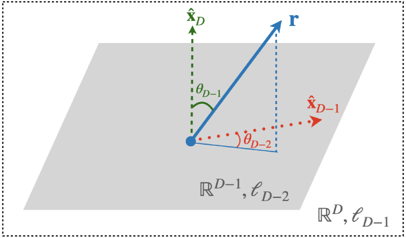
Figure 1: Cartoon illustrating the coordinate system used in this work, assuming a Euclidean geometry. The outer dashed box indicates $\mathbb{R}^{D}$, whilst the gray plane represents $\mathbb{R}^{D-1}$, containing the Cartesian coordinates $\{x_{1},\ldots,x_{D-1}\}$. The position vector $\mathbf{r}\in\mathbb{R}^{D}$ can be expressed in hyperspherical coordinates $\{r,\theta_{1},\ldots,\theta_{D-1}\}$, where $r$ is a radial coordinate. $\theta_{K-1}$ is defined as angle between the $\hat{\mathbf{x}}_{K}$ axis and the projection of $\mathbf{r}$ into the subspace $\mathbb{R}^{K}$, as shown for $\theta_{D-1}$ and $\theta_{D-2}$. The angles obey the restrictions $\theta_{K}\in[0,\pi)$ for $K>1$, and $\theta_{1}\in[0,2\pi)$. Each angle can be associated with an angular momentum index $\ell_{K-1}$, encoding the orbital angular momentum in the subspace $\mathbb{R}^{K}$ in which only the first $K$ Cartesian coordinates are varied (§1). $\ell_{1}$ gives the azimuthal angular momentum in the subspace containing $\{x_{1},x_{2},x_{3}\}$, and $\ell_{D-1}$ gives the total angular momentum.

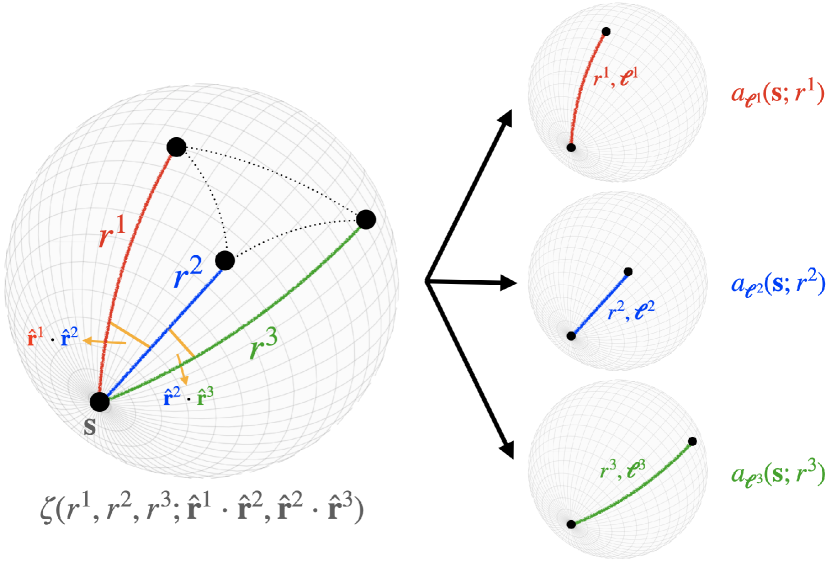
Figure 2: Sketch of the decomposition underlying our NPCF algorithm, visualized for $N=4$ in a 2D spherical geometry. On the left, we show the (rotation-averaged) 4PCF defined by three distances, $r^{1}$, $r^{2}$, $r^{3}$, and two angles $\hat{\mathbf{r}}^{1}\cdot\hat{\mathbf{r}}^{2}$, $\hat{\mathbf{r}}^{2}\cdot\hat{\mathbf{r}}^{3}$, relative to a primary position $\mathbf{s}$; naïve 4PCF estimation from $n$ particles proceeds by summing over each of the possible $n^{4}$ sets of points. On the right, we show our decomposition, factorizing the 4PCF into three functions of two positions, $a_{\boldsymbol{\ell}}(\mathbf{s};r)$, which may be independently estimated from the data-set, requiring consideration of only $n^{2}$ pairs of particles. Each function depends on a side length $r^{i}$ and a set of angular momentum indices $\boldsymbol{\ell}^{i}$; the latter specifies $\hat{\mathbf{r}}^{i}$ in the hyperspherical harmonic basis. This permits the NPCF components to be estimated by an algorithm with $\mathcal{O}(n^{2})$ complexity.

1 Single-Particle Basis

We begin by discussing the angular basis for functions of one position in $\mathbb{M}^{D}$, hereafter referred to as the ‘single-particle’ basis. In §2, the basis will allow construction of a joint basis of $(N-1)$ positions onto which the NPCF can be projected.

1.1 Constant-Curvature Metric

To form an efficient angular basis, we require the underlying manifold to be (a) homogeneous, and (b) isotropic. This leads to the well-known line-element

$$d\Sigma^{2}_{\mathbb{M}^{D}}=dr^{2}+\chi_{k}^{2}(r)\left\{d\theta_{D-1}^{2}+\sin^{2}\theta_{D-1}\left[d\theta_{D-2}^{2}+\sin^{2}\theta_{D-2}\left(d\theta_{D-3}^{2}+\cdots\right)\right]\right\}$$ (6)

(e.g., 17), adopting hyperspherical coordinates $\mathbf{r}\equiv\{r,\theta_{1},\ldots,\theta_{D-1}\}$. In this parametrization, $r$ is a radial coordinate, whilst the $\theta_{i}$ are angular variables, with $\theta_{1}\in[0,2\pi)$ (often denoted by $\phi$ in $D=3$) and $\theta_{j}\in[0,\pi)$ for $j>1$. A sketch of the coordinates is shown in Fig. 2 for a Euclidean geometry. (6) is a constant-curvature metric, specified by $\chi_{k}(r)=\sin\left(r\sqrt{k}\right)/\sqrt{k}$ if $|k|>0$ and $\chi_{k}(r)=r$ else. Here, $k>0$ gives the $D$-sphere, $\mathbb{S}^{D}$, $k<0$ leads to the hyperbolic geometry $\mathbb{H}^{D}$, and $k=0$ results in a Euclidean geometry $\mathbb{R}^{D}$. Such manifolds are ubiquitous in the physical sciences; for instance, this describes the spatial part of the Friedmann-Lemaître-Robertson-Walker metric for an expanding Universe (18).

1.2 Hyperspherical Harmonics

A convenient basis for the constant-curvature space $\mathbb{M}^{D}$ is formed from the set of harmonic functions $H:\mathbb{M}^{D}\to\mathbb{C}$. These satisfy the Laplace-Beltrami equation

$$\Delta H(\mathbf{r})\equiv\frac{1}{\sqrt{|g|}}\partial_{i}\left(\sqrt{|g|}\;g^{ij}\partial_{j}H(\mathbf{r})\right)=0,$$ (7)

where $H$ is twice continuously differentiable, $g$ is the metric (with $|g|=\mathrm{det}\left[g_{ij}\right]$), $i\in\{1,2,\ldots,D\}$ and we have assumed the Einstein summation convention. Assuming the metric of (6), (7) permits a separable solution of the form $H(\mathbf{r})=R(r)Y(\hat{\mathbf{r}})$, where $\hat{\mathbf{r}}=\{\theta_{1},\ldots,\theta_{D-1}\}$. The angular part of this must satisfy the following eigenfunction equation for constant $\lambda_{D-1}$:

$$\Delta_{\mathbb{S}^{D-1}}Y(\hat{\mathbf{r}})=-\lambda_{D-1}Y(\hat{\mathbf{r}}),$$ (8)

where $\Delta_{\mathbb{S}^{D-1}}$ is the Laplace-Beltrami operator on the $(D-1)$-sphere, given explicitly in (48). The corresponding solutions are the hyperspherical harmonics on $\mathbb{S}^{D-1}$ (e.g., 19, 20, 21). Since the harmonic functions are separable, the hyperspherical harmonics form an angular basis for any function on $\mathbb{M}^{D}$, regardless of the spatial curvature $k$. Physically, this decomposition is guaranteed since we have assumed the metric to be homogeneous and isotropic, enforcing invariance under the rotation group $SO(D)$ about any origin.

For a given dimension $D$, the hyperspherical harmonics, denoted $Y_{\ell_{1}\ldots\ell_{D-1}}(\hat{\mathbf{r}})$, may be obtained by solving (8) recursively, as detailed in Appendix A. These depend on a set of $(D-1)$ integers, $\{\ell_{k}\}$, which are related to angular momentum (cf. §11.3), and satisfy the selection rules

$$-\ell_{2}\leq\ell_{1}\leq\ell_{2},\quad\ell_{K-1}\leq\ell_{K}\leq\ell_{K+1}\quad(2\leq K\leq D-1).$$ (9)

In two- and three-dimensions, the hyperspherical harmonics take a simple form:

$$Y_{\ell_{1}}(\theta_{1})=\frac{1}{\sqrt{2\pi}}\,e^{i\ell_{1}\theta_{1}},\qquad Y_{\ell_{1}\ell_{2}}(\theta_{1},\theta_{2})=\sqrt{\frac{2\ell_{2}+1}{4\pi}\frac{(\ell_{2}+\ell_{1})!}{(\ell_{2}-\ell_{1})!}}\,e^{i\ell_{1}\theta_{1}}P_{\ell_{2}}^{-\ell_{1}}(\cos\theta_{2}),$$ (10)

for associated Legendre polynomials $P_{\ell}^{m}$. The $D=3$ functions are the usual spherical harmonics (in the Condon-Shortley convention), made clear by the identification $(\ell_{1},\ell_{2})\to(m,\ell)$, $(\theta_{1},\theta_{2})\to(\phi,\theta)$, where $\phi$ is the azimuthal angle. The explicit form of the hyperspherical harmonics for general $D$ is given in (50).

1.3 Connection to Angular Momentum Eigenstates

In 3D, the theory of angular momentum is centered around two operators, $\widehat{L}^{2}$ and $\widehat{L}_{3}$, which respectively give the total angular momentum and that projected onto the $\hat{\mathbf{x}}_{3}$ axis. Both may be constructed from the vector operator $\widehat{\mathbf{L}}=\mathbf{r}\times\mathbf{p}$, where $p_{j}=-i(\partial/\partial x^{j})$ is the linear momentum in $\mathbb{R}^{3}$. For $D\neq 3$, we cannot define a cross-product, thus we instead start from the tensorial angular momentum operator, following (22):

$$\widehat{\mathsf{L}}_{ij}=x_{i}p_{j}-x_{j}p_{i},\quad i\neq j\in\{1,2,\ldots,D\}$$ (11)

where $\{x_{1},\ldots,x_{D}\}$ is a Cartesian coordinate chart. These operators are antisymmetric ($\widehat{\mathsf{L}}_{ij}=-\widehat{\mathsf{L}}_{ji}$) and form the Lie algebra $\mathfrak{so}(D)$, i.e. that of the rotation group in $D$ dimensions. Of particular interest is $\widehat{\mathsf{L}}_{12}$; when applied to some state, this gives the azimuthal angular momentum in the subspace containing $\{x_{1},x_{2},x_{3}\}$, just as for $\widehat{L}_{3}$ in $D=3$.

To fully define the rotational properties of a single-particle function in $D$-dimensional space, we must specify not only its total angular momentum, but also that projected into lower-dimensional subspaces. These can be obtained from the operators

$$\widehat{\mathcal{L}}^{2}_{K}\equiv\sum_{i=1}^{K}\sum_{j=i+1}^{K}(\widehat{\mathsf{L}}_{ij})^{2},$$ (12)

for $K\geq 3$. Here, $\widehat{\mathcal{L}}^{2}_{3}\equiv(\widehat{\mathsf{L}}_{12})^{2}+(\widehat{\mathsf{L}}_{13})^{2}+(\widehat{\mathsf{L}}_{23})^{2}$ gives the angular momentum in the subspace $\{x_{1},x_{2},x_{3},0,\ldots,0\}$ of $\mathbb{R}^{D}$, $\widehat{\mathcal{L}}^{2}_{4}$ gives that in the subspace $\{x_{1},x_{2},x_{3},x_{4},0,\ldots,0\}$ et cetera. $\widehat{\mathcal{L}}_{D}^{2}$ is the total angular momentum operator, analogous to $\widehat{L}^{2}$ in the three-dimensional theory.

As shown in (22, Ch. 3), a complete set of commuting angular momentum operators is given by $\{\widehat{\mathsf{L}}_{12}$, $\widehat{\mathcal{L}}_{3}^{2},\ldots,\widehat{\mathcal{L}}_{D}^{2}\}$. Moreover, the hyperspherical harmonics of §11.2 are simultaneous eigenfunctions of these, satisfying

$$\widehat{\mathsf{L}}_{12}Y_{\ell_{1}\ldots\ell_{D-1}}(\hat{\mathbf{r}}) = \ell_{1}\,Y_{\ell_{1}\ldots\ell_{D-1}}(\hat{\mathbf{r}}),\qquad\widehat{\mathcal{L}}^{2}_{K}Y_{\ell_{1}\ldots\ell_{D-1}}(\hat{\mathbf{r}})=\ell_{K-1}(\ell_{K-1}+K-2)\,Y_{\ell_{1}\ldots\ell_{D-1}}(\hat{\mathbf{r}})\quad(3\leq K\leq D).$$ (13)

We may thus associate $\ell_{K-1}$ with the orbital angular momentum in the subspace comprising the first $K$ Cartesian coordinates (for $K\geq 3)$, and $\ell_{1}$ with that projected onto the $\hat{\mathbf{x}}_{3}$ axis. Such an interpretation also justifies the conditions in (9); projections of the angular momentum into lower-dimensional spaces must have equal or lesser magnitudes than the total angular momentum in $D$ dimensions.

For later use, we introduce abstract notation for the angular momentum basis functions, writing $Y_{\ell_{1}\ldots\ell_{D-1}}(\hat{\mathbf{r}})\to\left|{\ell_{1}\ldots\ell_{D-1}}\right\rangle$ in Dirac (or bra-ket) notation. In total, there are $\binom{\ell_{D-1}+D-3}{D-3}(2\ell_{D-1}+D-2)/(D-2)$ eigenstates corresponding to a given total angular momentum $\ell_{D-1}$ if $D\geq 3$, and one if $D=2$ (22, Eq. 3.37). For a suitably defined inner product, the basis functions are orthonormal (23, 20, 21):

$$\int_{\mathbb{S}^{D-1}}d\Omega_{D-1}Y^{*}_{\ell_{1}\ldots\ell_{D-1}}(\hat{\mathbf{r}})Y_{\ell_{1}^{\prime}\ldots\ell^{\prime}_{D-1}}(\hat{\mathbf{r}})\equiv\left\langle\left.{\ell_{1}\ldots\ell_{D-1}}\right|{\ell_{1}^{\prime}\ldots\ell^{\prime}_{D-1}}\right\rangle=\delta^{\rm K}_{\ell_{1}\ell_{1}^{\prime}}\ldots\delta^{\rm K}_{\ell_{D-1}\ell_{D-1}^{\prime}},$$ (14)

where the Kronecker delta, $\delta^{\rm K}_{ij}$, is unity if $i=j$ and zero otherwise. Furthermore, they form a complete basis on $\mathbb{S}^{D-1}$, such that, for any $h:\mathbb{S}^{D-1}\to\mathbb{C}$

$$\left|{h}\right\rangle=\sum_{\ell_{1}\ldots\ell_{D-1}}\left\langle\left.{\ell_{1}\ldots\ell_{D-1}}\right|{h}\right\rangle\left|{\ell_{1}\ldots\ell_{D-1}}\right\rangle\quad\leftrightarrow\quad,h(\hat{\mathbf{r}})=\sum_{\ell_{1}\ldots\ell_{D-1}}h_{\ell_{1}\ldots\ell_{D-1}}Y_{\ell_{1}\ldots\ell_{D-1}}(\hat{\mathbf{r}})$$ (15)

where the summation runs over all angular momentum indices allowed by the selection rules of (9). The basis coefficients $h_{\ell_{1}\ldots\ell_{D-1}}=\left\langle\left.{\ell_{1}\ldots\ell_{D-1}}\right|{h}\right\rangle$ may be obtained via orthonormality. Since the angular part of $\mathbb{M}^{D}$ is just the $(D-1)$-sphere $\mathbb{S}^{D-1}$ (§11.1), any one-particle function on $\mathbb{M}^{D}$ can be decomposed into this basis; in general, the coefficients retain dependence on the radial coordinate $r$.

2 $(N-1)$-Particle Basis

We now utilize the mathematics of angular momentum addition to generalize the angular basis of §1 to functions of $(N-1)$ positions, i.e. $f:\left(\mathbb{M}^{D}\right)^{\otimes(N-1)}\to\mathbb{C}$.

2.1 Angular Momentum Addition

To begin, we consider the combination of two angular basis functions on the $(D-1)$-sphere. For convenience, we will work in the Dirac representation and denote the set of angular momentum indices by $\boldsymbol{\ell}\equiv\{\ell_{1},\ldots,\ell_{D-1}\}$, with superscripts used to distinguish between particles. Given single-particle states $\left|{\boldsymbol{\ell}^{1}}\right\rangle$ and $\left|{\boldsymbol{\ell}^{2}}\right\rangle$, the simplest two-particle state is $\left|{\boldsymbol{\ell}^{1},\boldsymbol{\ell}^{2}}\right\rangle\equiv\left|{\boldsymbol{\ell}^{1}}\right\rangle\left|{\boldsymbol{\ell}^{2}}\right\rangle$, which exists in the product space $\mathbb{S}^{D-1}\otimes\mathbb{S}^{D-1}$. This is a simultaneous eigenstate of angular momentum operators for the first and second particles, $\widehat{\mathsf{L}}_{ij}^{(1)}$ and $\widehat{\mathsf{L}}_{ij}^{(2)}$ (cf. §11.3). Whilst the product states $\left|{\boldsymbol{\ell}^{1},\boldsymbol{\ell}^{2}}\right\rangle$ do form a basis on $\mathbb{S}^{D-1}\otimes\mathbb{S}^{D-1}$ (sometimes called the ‘uncoupled basis’ (24)), it is not an efficient one, since (a) we require $2(D-1)$ angular momentum indices to specify the state, which, as shown below, is considerably more than necessary, and (b) the indices are not straightforwardly connected to the joint rotation properties of the two-particle state.

A more appropriate basis is wrought by considering the combined angular momentum operator $\widehat{\mathsf{L}}_{ij}^{(12)}\equiv\widehat{\mathsf{L}}_{ij}^{(1)}+\widehat{\mathsf{L}}_{ij}^{(2)}$, which specifies the properties of some two-particle function, $f(\mathbf{r}^{1},\mathbf{r}^{2})$, under joint rotations of $\mathbf{r}^{1}$ and $\mathbf{r}^{2}$ about a common origin. As in §11.3, $\widehat{\mathsf{L}}_{ij}^{(12)}$ may be used to construct a set of commuting angular momentum operators, whose eigenstates can be written $\left|{\boldsymbol{L}}\right\rangle\equiv\left|{L_{1}\ldots L_{D-1}}\right\rangle$. Here, $L_{K-1}$ specifies the combined angular momentum projected into the $K$-dimensional subspace in which the first $K$ Cartesian coordinates are varied (for $K\geq 3$), and $L_{1}$ gives that projected onto the $\hat{\mathbf{x}}_{3}^{1},\hat{\mathbf{x}}_{3}^{2}$ axes. Similarly to the single-particle state, the $\boldsymbol{L}$ indices must obey the selection rules of (9).

Two-particle states of definite combined angular momentum are formed by summing over products of one-particle states, just as in the 3D case (e.g., (25, 26), see also (27, 28, 24) for a discussion with more general $D$). Explicitly, they are given by

$$\boxed{\left|{\ell_{D-1}^{1}\;\ell_{D-1}^{2};\boldsymbol{L}}\right\rangle=\sum_{\ell_{1}^{1}\ldots\ell^{1}_{D-2}}\sum_{\ell_{2}^{2}\ldots\ell^{2}_{D-2}}\left\langle\left.{\boldsymbol{\ell}^{1}},{\boldsymbol{\ell}^{2}}\right|{\boldsymbol{L}}\right\rangle\left|{\boldsymbol{\ell}^{1}}\right\rangle\left|{\boldsymbol{\ell}^{2}}\right\rangle,}$$ (16)

where $\left\langle\left.{\boldsymbol{\ell}^{1}},{\boldsymbol{\ell}^{2}}\right|{\boldsymbol{L}}\right\rangle$ is a Clebsch-Gordan (hereafter CG) coefficient (e.g., 29). This is often referred to as the ‘coupled basis’ (24). To uniquely define the state, we must specify (a) the combined angular momentum eigenvalues $\boldsymbol{L}$, and (b) the total angular momentum of the first and second particle, $\ell_{D-1}^{1}$ and $\ell_{D-1}^{2}$. Importantly, (16) involves a sum over $\{\ell_{1}^{i},\ldots,\ell_{D-2}^{i}\}$, i.e. the projection of the particles’ angular momentum into lower-dimensional subspaces. Due to this, the combined state is specified by only $(D+1)$ indices, which, for $D>3$, is significantly fewer than the $2(D-1)$ required for $\left|{\boldsymbol{\ell}^{1},\boldsymbol{\ell}^{2}}\right\rangle$.

Practically, one must know the CG coefficients $\left\langle\left.{\boldsymbol{\ell}^{1}},{\boldsymbol{\ell}^{2}}\right|{\boldsymbol{L}}\right\rangle$ in order to form the coupled basis of (16). These have been studied in depth (e.g., 30, 25, 26, 29, 31, 32) and may be simplified by techniques such as Racah’s factorization lemma (33). One route to their computation is via (16); starting from a state of maximal combined angular momentum, $\left|{\ell_{D-1}^{1}\ell_{D-1}^{2};\boldsymbol{\ell}^{1}+\boldsymbol{\ell}^{2}}\right\rangle\equiv\left|{\boldsymbol{\ell}^{1}}\right\rangle\left|{\boldsymbol{\ell}^{2}}\right\rangle$ (wherein the two angular momentum vectors in $\mathbb{R}^{D}$ are aligned), ladder operators may be applied iteratively to obtain states of lower angular momentum, whose weightings give the CG coefficients. As in (26, 25), the explicit forms for the CG coefficients in $D=2$ and $D=3$ are given by

$$\left\langle\left.{\ell^{1}},{\ell^{2}}\right|{L}\right\rangle=\delta^{\rm K}_{(\ell^{1}+\ell^{2})L},\qquad\left\langle\left.{\ell^{1}_{1}\ell^{1}_{2}},{\ell_{1}^{2}\ell_{2}^{2}}\right|{L_{1}L_{2}}\right\rangle=(-1)^{-\ell_{2}^{1}+\ell_{2}^{2}-L_{1}}\sqrt{2L_{2}+1}\begin{pmatrix}{\ell_{2}^{1}}&{\ell_{2}^{2}}&{L_{2}}\\ {\ell_{1}^{1}}&{\ell_{1}^{2}}&{-L_{1}}\end{pmatrix},$$ (17)

where the $2\times 3$ matrix is a Wigner 3-$j$ symbol (e.g., 34, §34). The $D=4$ case is similar (see 30, 29, 35), but includes a Wigner 9-$j$ symbol.

CG coefficients satisfy certain orthogonality conditions, including

$$\sum_{\ell^{1}_{1}\ldots\ell_{D-2}^{1}}\sum_{\ell^{2}_{1}\ldots\ell^{2}_{D-2}}\left\langle\left.{\boldsymbol{\ell}^{1}},{\boldsymbol{\ell}^{2}}\right|{\boldsymbol{L}}\right\rangle\left\langle\left.{\boldsymbol{\ell}^{1}},{\boldsymbol{\ell}^{2}}\right|{\boldsymbol{L}^{\prime}}\right\rangle=\delta^{\rm K}_{L_{1}L_{1}^{\prime}}\times\cdots\times\delta^{\rm K}_{L_{D-1}L_{D-1}^{\prime}}.$$ (18)

Coupled with the orthonormality of the one-particle states $\left|{\boldsymbol{\ell}}\right\rangle$ (Eq. 24), this ensures that the combined-angular-momentum basis is orthonormal, i.e.

$$\left\langle\left.{l^{1}_{D-1}l^{2}_{D-1};\boldsymbol{L}^{\prime}}\right|{\ell^{1}_{D-1}\ell_{D-1}^{2};\boldsymbol{L}}\right\rangle=\left(\delta^{\rm K}_{L_{1}L_{1}^{\prime}}\cdots\delta^{\rm K}_{L_{D-1}L^{\prime}_{D-1}}\right)\times\left(\delta^{\rm K}_{\ell^{1}_{D-1}l^{1}_{D-1}}\delta^{\rm K}_{\ell_{D-1}^{2}l_{D-1}^{2}}\right).$$ (19)

Furthermore, $\left\langle\left.{\boldsymbol{\ell}^{1}},{\boldsymbol{\ell}^{2}}\right|{\boldsymbol{L}}\right\rangle$ is non-zero only if the following conditions are satisfied:

$$L_{1}=\ell^{1}_{1}+\ell^{2}_{1},\quad|\ell^{1}_{K}-\ell^{2}_{K}|\leq L_{K}\leq\ell^{1}_{K}+\ell^{2}_{K},\quad(2\leq K\leq D-1).$$ (20)

The first constraint occurs since $L_{1}$ is the eigenvalue corresponding to $\widehat{\mathsf{L}}^{(12)}_{12}$, which is linear in $\widehat{\mathsf{L}}_{12}^{(1)}$ and $\widehat{\mathsf{L}}_{12}^{(2)}$ (cf. addition of $m$ indices in 3D), and the second is due to the triangle inequality, recalling that $L_{K}$ corresponds to the magnitude of the angular momentum in the subspace $\mathbb{R}^{K}$. In particular, the constraints fix the total combined angular momentum, $L_{D-1}$, to be no greater than $\ell_{D-1}^{1}+\ell_{D-1}^{2}$.

2.2 Combined Angular Momentum Basis

By repeated application of the angular momentum addition rule (Eq. 16), we may build up an $(N-1)$-particle state of definite combined angular momentum. First, we combine $\left|{\boldsymbol{\ell}^{1}}\right\rangle$ and $\left|{\boldsymbol{\ell}^{2}}\right\rangle$ to form the two-particle state $\left|{\ell^{1}_{D-1}\ell^{2}_{D-1};\boldsymbol{\ell}^{12}}\right\rangle$, which is then combined with $\boldsymbol{\ell}^{3}$ to form the three-particle state $\left|{\ell^{1}_{D-1}\ell^{2}_{D-1}\ell^{12}_{D-1}\ell^{3}_{D-1};\boldsymbol{\ell}^{123}}\right\rangle$, et cetera. In full, we obtain the $(N-1)$-particle basis function

$$\boxed{\left|{{\boldsymbol{\Lambda}};\boldsymbol{L}}\right\rangle=\sum_{[\boldsymbol{\ell}^{1}][\boldsymbol{\ell}^{2}]\ldots[\boldsymbol{\ell}^{N-1}]}C^{{\boldsymbol{\Lambda}};\boldsymbol{L}}_{\boldsymbol{\ell}^{1}\boldsymbol{\ell}^{2}\ldots\boldsymbol{\ell}^{N-1}}\left|{\boldsymbol{\ell}^{1}}\right\rangle\left|{\boldsymbol{\ell}^{2}}\right\rangle\cdots\left|{\boldsymbol{\ell}^{N-1}}\right\rangle,}$$ (21)

summing over all intermediate angular momenta $\ell_{k}^{i}$ with $k<(D-1)$, as denoted by $[\boldsymbol{\ell}^{i}]$. The combined state in (21) is specified by the set of total angular momentum indices ${\boldsymbol{\Lambda}}\equiv\{\ell^{1}_{D-1},\ell_{D-1}^{2},\ell_{D-1}^{12},\ell^{3}_{D-1},\ell^{123}_{D-1},\ell^{4}_{D-1},\ldots,\ell_{D-1}^{12\ldots(N-2)},\ell_{D-1}^{{N-1}}\}$ and involves the coupling coefficients

$$C^{{\boldsymbol{\Lambda}};\boldsymbol{L}}_{\boldsymbol{\ell}^{1}\boldsymbol{\ell}^{2}\ldots\boldsymbol{\ell}^{{N-1}}}=\sum_{[\boldsymbol{\ell}^{12}]\ldots[\boldsymbol{\ell}^{12\ldots(N-2)}]}\left\langle\left.{\boldsymbol{\ell}^{1}},{\boldsymbol{\ell}^{2}}\right|{\boldsymbol{\ell}^{12}}\right\rangle\left\langle\left.{\boldsymbol{\ell}^{12}},{\boldsymbol{\ell}^{3}}\right|{\boldsymbol{\ell}^{123}}\right\rangle\cdots\left\langle\left.{\boldsymbol{\ell}^{12\ldots(N-2)}},{\boldsymbol{\ell}^{N-1}}\right|{\boldsymbol{L}}\right\rangle,$$ (22)

which is a product of CG symbols. We have additionally set $\boldsymbol{\ell}^{12\ldots(N-1)}\equiv\boldsymbol{L}$, representing the combined angular momentum eigenvalues. Note that (21) contains a sum over both the primary indices $\ell^{i}$ (which define the single-particle states) and intermediates, e.g., $\ell^{12\ldots}$ (within the coupling definitions), but not those corresponding to total angular momenta, i.e. $\ell_{D-1}$.

The meaning of (21) is straightforward; an $(N-1)$-particle state with combined angular momentum $\boldsymbol{L}$ can be obtained as a sum of product states, weighted by $(N-2)$ CG coefficients. To define the state uniquely, we must specify not only the total angular momentum $\ell_{D-1}$ of each single-particle state, but also the total angular momentum of the intermediate states, e.g., $\ell_{D-1}^{12}$ arising from the coupling of $\left|{\boldsymbol{\ell}^{1}}\right\rangle$ and $\left|{\boldsymbol{\ell}^{2}}\right\rangle$. In total, the state is specified by $(2N+D-5)$ indices; again significantly fewer than the $(N-1)(D-1)$ required for the product state $\left|{\boldsymbol{\ell}^{1}}\right\rangle\cdots\left|{\boldsymbol{\ell}^{N-1}}\right\rangle$.

A particularly interesting state is that of zero combined angular momentum, i.e. $\boldsymbol{L}=\boldsymbol{0}$. From (21), this is simply

$$\boxed{\left|{{\boldsymbol{\Lambda}};\boldsymbol{0}}\right\rangle=\sum_{[\boldsymbol{\ell}^{1}]\ldots[\boldsymbol{\ell}^{N-1}]}C^{{\boldsymbol{\Lambda}};\boldsymbol{0}}_{\boldsymbol{\ell}^{1}\ldots\boldsymbol{\ell}^{{N-1}}}\left|{\boldsymbol{\ell}^{1}}\right\rangle\left|{\boldsymbol{\ell}^{2}}\right\rangle\cdots\left|{\boldsymbol{\ell}^{N-1}}\right\rangle.}$$ (23)

Unlike the general state (Eq. 21), this is involves only $(N-4)$ intermediate couplings $\boldsymbol{\ell}^{12\ldots}$, since the final CG coefficient in (22) fixes $\ell^{12\ldots(N-2)}_{1}=-\ell_{1}^{N-1}$ and $\ell^{12\ldots(N-2)}_{K}=\ell_{K}^{N-1}$ for $K>1$. In total, this requires $(2N-5)$ indices to fully specify, regardless of dimension.

2.3 $(N-1)$-Particle Basis Properties

The $(N-1)$-particle basis functions of Eqs. 21 & 23 have analogous properties to those of the single-particle basis (cf. §11.3). Using (18), we can show orthonormality:

$$\left\langle\left.{{\boldsymbol{\Lambda}}^{\prime};\boldsymbol{L}^{\prime}}\right|{{\boldsymbol{\Lambda}};\boldsymbol{L}}\right\rangle=\delta^{\rm K}_{{\boldsymbol{\Lambda}}{\boldsymbol{\Lambda}}^{\prime}}\delta^{\rm K}_{\boldsymbol{L}\boldsymbol{L}^{\prime}}$$ (24)

requiring equality of both the combined angular momentum vectors ($\boldsymbol{L}$ and $\boldsymbol{L}^{\prime}$) and all components of ${\boldsymbol{\Lambda}}$ and ${\boldsymbol{\Lambda}}^{\prime}$. Since the angular momentum states form a complete basis, any $(N-1)$-particle function $h:\left(\mathbb{S}^{D-1}\right)^{\otimes(N-1)}$ can be decomposed into a sum of basis states:

$$\left|{h}\right\rangle=\sum_{\boldsymbol{L}}\sum_{{\boldsymbol{\Lambda}}}\left\langle\left.{{\boldsymbol{\Lambda}};\boldsymbol{L}}\right|{h}\right\rangle\left|{{\boldsymbol{\Lambda}};\boldsymbol{L}}\right\rangle\quad\leftrightarrow\quad h(\hat{\mathbf{r}}^{1},\ldots,\hat{\mathbf{r}}^{N-1})=\sum_{\boldsymbol{L}}\sum_{{\boldsymbol{\Lambda}}}h_{\boldsymbol{\Lambda}}^{\boldsymbol{L}}\mathcal{P}_{\boldsymbol{\Lambda}}^{\boldsymbol{L}}(\hat{\mathbf{r}}^{1},\ldots,\hat{\mathbf{r}}^{N-1})$$ (25)

summing over both combined angular momentum indices $\boldsymbol{L}$ and the indices contained within ${\boldsymbol{\Lambda}}$ (analogously to Eq. 15). The basis components are denoted by $\left\langle\left.{{\boldsymbol{\Lambda}};\boldsymbol{L}}\right|{h}\right\rangle\equiv h_{{\boldsymbol{\Lambda}}}^{\boldsymbol{L}}$. For the second equality, we switch to wavefunction notation, with the basis functions defined as (cf. Eq. 21)

$$\boxed{\mathcal{P}_{\boldsymbol{\Lambda}}^{\boldsymbol{L}}(\hat{\mathbf{r}}^{1},\ldots,\hat{\mathbf{r}}^{N-1})=\sum_{[\boldsymbol{\ell}^{1}][\boldsymbol{\ell}^{2}]\ldots[\boldsymbol{\ell}^{N-1}]}C^{{\boldsymbol{\Lambda}};\boldsymbol{L}}_{\boldsymbol{\ell}^{1}\boldsymbol{\ell}^{2}\ldots\boldsymbol{\ell}^{N-1}}Y_{\boldsymbol{\ell}^{1}}(\hat{\mathbf{r}}^{1})Y_{\boldsymbol{\ell}^{2}}(\hat{\mathbf{r}}^{2})\cdots Y_{\boldsymbol{\ell}^{N-1}}(\hat{\mathbf{r}}^{N-1}),}$$ (26)

where $Y_{\boldsymbol{\ell}}(\hat{\mathbf{r}})$ are the hyperspherical harmonics of §11.2. Since $\mathbb{S}^{D-1}$ is the angular part of $\mathbb{M}^{D}$, the directional dependence of any $(N-1)$-particle function in $\mathbb{M}^{D}$ can be expanded in the separable form of Eq. 25.

If the function $h$ appearing in (25) has rotational symmetry, a simpler decomposition is possible. In particular, we assume it to be invariant under rotations drawn from the subspace $\{x_{1},\ldots,x_{K},0,\ldots,0\}$ of $SO(D)$. An example of this would be azimuthal symmetry in $D=3$; here, the system is invariant under rotations about one axis only. To obey rotational symmetry in $K$ dimensions, the basis functions must satisfy

$$\widehat{\mathcal{L}}^{2}_{K}\left|{{\boldsymbol{\Lambda}};\boldsymbol{L}}\right\rangle=0\quad\Rightarrow\quad L_{i}=0,\quad\forall\,i<K,$$ (27)

where $\widehat{\mathcal{L}}^{2}_{K}$ is the combined angular momentum operator (Eq. 12). In this instance, only basis functions of the form $\left|{{\boldsymbol{\Lambda}};0\ldots 0\;L_{K}\ldots L_{D-1}}\right\rangle$ enter into (25), reducing the number of basis coefficients from approximately $\left(\ell_{D-1}^{\rm max}\right)^{2N+D-5}$ to $\left(\ell_{D-1}^{\rm max}\right)^{2N+D-K-5}$, for maximum multipole $\ell_{D-1}^{\rm max}$. If $h$ is invariant under spatial rotations about any axis (i.e. it is isotropic), only the $\boldsymbol{L}=\boldsymbol{0}$ state is required. In this case

$$\left|{h}\right\rangle = \sum_{{\boldsymbol{\Lambda}}}\left\langle\left.{{\boldsymbol{\Lambda}};\boldsymbol{0}}\right|{h}\right\rangle\left|{{\boldsymbol{\Lambda}};\boldsymbol{0}}\right\rangle\quad\leftrightarrow\quad h(\hat{\mathbf{r}}^{1},\ldots,\hat{\mathbf{r}}^{N-1})=\sum_{{\boldsymbol{\Lambda}}}h_{{\boldsymbol{\Lambda}}}^{\boldsymbol{0}}\mathcal{P}_{\boldsymbol{\Lambda}}^{\boldsymbol{0}}(\hat{\mathbf{r}}^{1},\ldots,\hat{\mathbf{r}}^{N-1}),$$ (28)

for components $h_{{\boldsymbol{\Lambda}}}^{\boldsymbol{0}}\equiv\left\langle\left.{{\boldsymbol{\Lambda}};\boldsymbol{0}}\right|{h}\right\rangle$, which may be determined via orthonormality. The directional dependence of any isotropic $(N-1)$-particle function in $\mathbb{M}^{D}$ can be expanded in the separable form of Eq. 28.

For $N=3$ and $N=4$, the isotropic basis functions take the explicit forms:

$$\mathcal{P}_{\ell_{D-1}}^{\boldsymbol{0}}(\hat{\mathbf{r}}^{1},\hat{\mathbf{r}}^{2}) = \sum_{\ell_{1}\ldots\ell_{D-2}}Y_{\ell_{1}\ell_{2}\ldots\ell_{D-1}}(\hat{\mathbf{r}}^{1})Y_{(-\ell_{1})\ell_{2}\ldots\ell_{D-1}}(\hat{\mathbf{r}}^{2}),$$ (29)

$$\mathcal{P}_{\ell^{1}_{D-1}\ell^{2}_{D-1}\ell^{3}_{D-1}}^{\boldsymbol{0}}(\hat{\mathbf{r}}^{1},\hat{\mathbf{r}}^{2},\hat{\mathbf{r}}^{3}) = \sum_{\ell_{1}^{1}\ldots\ell^{1}_{D-2}}\sum_{\ell^{2}_{1}\ldots\ell^{2}_{D-2}}\sum_{\ell_{1}^{3}\ldots\ell^{3}_{D-2}}\left\langle\left.{\boldsymbol{\ell}^{1}},{\boldsymbol{\ell}^{2}}\right|{(-\ell^{3}_{1})\ell_{2}^{3}\ldots\ell_{D-1}^{3}}\right\rangle Y_{\ell_{1}^{1}\ldots\ell^{1}_{D-1}}(\hat{\mathbf{r}}^{1})Y_{\ell_{1}^{2}\ldots\ell^{2}_{D-1}}(\hat{\mathbf{r}}^{2})Y_{\ell_{1}^{3}\ldots\ell^{3}_{D-1}}(\hat{\mathbf{r}}^{3}).$$

noting that the final CG coefficient is of the form $\left\langle\left.{\boldsymbol{\ell}^{12\ldots(N-2)}},{\boldsymbol{\ell}^{N-1}}\right|{\boldsymbol{0}}\right\rangle$, which enforces $\ell^{12\ldots(N-2)}_{1}+\ell^{N-1}_{1}=0$ and $\ell^{12\ldots(N-2)}_{K}=\ell^{N-1}_{K}$ for $K>1$. This is a natural extension of the Legendre polynomials to $D$ dimensions; indeed the $D=3$ case recovers the Legendre polynomial $\mathcal{L}_{\ell_{2}}(\hat{\mathbf{r}}^{1}\cdot\hat{\mathbf{r}}^{2})$ rescaled by $(-1)^{\ell_{2}}(4\pi)/\sqrt{2\ell_{2}+1}$ (cf. 36).

Finally, we note the properties of the basis functions under complex conjugation and parity inversion:

$$\left[\mathcal{P}_{\boldsymbol{\Lambda}}^{\boldsymbol{L}}(\hat{\mathbf{r}}^{1},\ldots,\hat{\mathbf{r}}^{{N-1}})\right]^{*} = (-1)^{L_{D-1}-L_{1}}(-1)^{\ell^{1}_{D-1}+\cdots+\ell^{N-1}_{D-1}}\mathcal{P}_{\boldsymbol{\Lambda}}^{\boldsymbol{0}}(\hat{\mathbf{r}}^{1},\ldots,\hat{\mathbf{r}}^{{N-1}})$$ (30)

$$\mathbb{P}\left[\mathcal{P}_{\boldsymbol{\Lambda}}^{\boldsymbol{L}}(\hat{\mathbf{r}}^{1},\ldots,\hat{\mathbf{r}}^{{N-1}})\right] = (-1)^{\ell_{D-1}^{1}+\cdots+\ell_{D-1}^{{N-1}}}\mathcal{P}_{\boldsymbol{\Lambda}}^{\boldsymbol{0}}(\hat{\mathbf{r}}^{1},\ldots,\hat{\mathbf{r}}^{{N-1}}),$$

using (51), noting that the CG coefficients enforce $\ell_{1}^{1}+\ell_{1}^{2}+\cdots+\ell_{1}^{N-1}+L_{1}=0$. For $\boldsymbol{L}=\boldsymbol{0}$, this implies that even-(odd-)parity basis functions are purely real (imaginary).

3 An Efficient Correlation Function Estimator

Armed with the $(N-1)$-particle angular basis of §2, we now proceed to construct an efficient estimator for the $N$-point correlation function components. For full generality, we do not assume the NPCF to have any rotational symmetry; such symmetries set various basis components to zero, as discussed in §22.3.

3.1 Derivation

Assuming statistical homogeneity, the NPCF defined in (1) is a function of $(N-1)$ points on $\mathbb{M}^{D}$, and may thus be expanded in the combined angular momentum basis of §2 (cf. Eq. 4):

$$\boxed{\zeta(\mathbf{r}^{1},\ldots,\mathbf{r}^{N-1})=\sum_{\boldsymbol{L}}\sum_{{\boldsymbol{\Lambda}}}\zeta^{\boldsymbol{L}}_{\boldsymbol{\Lambda}}(r^{1},\ldots,r^{N-1})\mathcal{P}_{{\boldsymbol{\Lambda}}}^{\boldsymbol{L}}(\hat{\mathbf{r}}^{1},\ldots,\hat{\mathbf{r}}^{N-1}),}$$ (31)

where the basis states, $\mathcal{P}_{\boldsymbol{\Lambda}}^{\boldsymbol{L}}$, are defined in (26). As before, we sum both over $\boldsymbol{L}$, which specifies the properties of the NPCF under joint rotations of all $(N-1)$ direction vectors (with only $\boldsymbol{L}=\boldsymbol{0}$ required if the NPCF is isotropic), and ${\boldsymbol{\Lambda}}\equiv\{\ell^{1}_{D-1},\ell_{D-1}^{2},\ell_{D-1}^{12},\ell^{3}_{D-1},\ell^{123}_{D-1},\ell^{4}_{D-1},\ldots,\ell_{D-1}^{{N-1}}\}$, which defines the relative orientations of the direction vectors. In this form, the NPCF is fully specified by the basis coefficients $\zeta^{\boldsymbol{L}}_{\boldsymbol{\Lambda}}$, which are functions only of the radial parameters $r^{i}$.

Due to the parity properties of the basis functions (Eq. 30), basis coefficients with even (odd) $\sum_{i=1}^{N-1}\ell_{D-1}^{i}$ represent even-parity (odd-parity) NPCF contributions; furthermore, they are purely real (imaginary) if the random field $X$ is real-valued and $\boldsymbol{L}=\boldsymbol{0}$. Parity-odd isotropic basis functions occur only for $N>D$; at lower orders, a parity transformation is equivalent to a rotation, under which the basis functions are invariant.

The basis coefficients can be extracted from (31) via an inner product:

$$\zeta_{\boldsymbol{\Lambda}}^{\boldsymbol{L}}(r^{1},\ldots,r^{N-1})\equiv\left\langle\left.{{\boldsymbol{\Lambda}};\boldsymbol{L}}\right|{\zeta}\right\rangle=\int_{\left(\mathbb{S}^{D-1}\right)^{\otimes(N-1)}}d\Omega_{D-1}^{1}\cdots d\Omega_{D-1}^{N-1}\,\left[\zeta(\mathbf{r}^{1},\ldots,\mathbf{r}^{N-1})\mathcal{P}_{\boldsymbol{\Lambda}}^{\boldsymbol{L},*}(\hat{\mathbf{r}}^{1},\ldots,\hat{\mathbf{r}}^{N-1})\right],$$ (32)

where the integral is over $(N-1)$ copies of the angular space. As in (2), the NPCF may be estimated as a product of $N$ random fields, integrated over space; inserted into (32) this yields

$$\hat{\zeta}^{\boldsymbol{L}}_{\boldsymbol{\Lambda}}(r^{1},\ldots,r^{N-1})=\frac{1}{V_{D}}\int_{\mathbb{M}^{D}}d^{D}\mathbf{s}\int_{\left(\mathbb{S}^{D-1}\right)^{\otimes(N-1)}}d\Omega_{D-1}^{1}\cdots d\Omega_{D-1}^{N-1}\,\left[X(\mathbf{s})X(\mathbf{s}+\mathbf{r}^{1})\cdots X(\mathbf{s}+\mathbf{r}^{N-1})\mathcal{P}_{\boldsymbol{\Lambda}}^{\boldsymbol{L},*}(\hat{\mathbf{r}}^{1},\ldots,\hat{\mathbf{r}}^{N-1})\right].$$ (33)

Finally, we insert the explicit forms of the $(N-1)$-particle basis functions (Eq. 26), which yields

$$\boxed{\hat{\zeta}^{\boldsymbol{L}}_{\boldsymbol{\Lambda}}(r^{1},\ldots,r^{N-1})=\frac{1}{V_{D}}\sum_{[\boldsymbol{\ell}^{1}]\ldots[\boldsymbol{\ell}^{N-1}]}C^{{\boldsymbol{\Lambda}};\boldsymbol{L}}_{\boldsymbol{\ell}^{1}\ldots\boldsymbol{\ell}^{N-1}}\int_{\mathbb{M}^{D}}d^{D}\mathbf{s}\,\left[X(\mathbf{s})a_{\boldsymbol{\ell}^{1}}(\mathbf{s};r^{1})\cdots a_{\boldsymbol{\ell}^{N-1}}(\mathbf{s};r^{N-1})\right],}$$ (34)

defining the functions

$$a_{\boldsymbol{\ell}}(\mathbf{s};r)\equiv\int_{\mathbb{S}^{D-1}}d\Omega_{D-1}\,X(\mathbf{s}+\mathbf{r})Y^{*}_{\boldsymbol{\ell}}(\hat{\mathbf{r}}).$$ (35)

Importantly, the angular integrals are now fully decoupled.

Usually, the NPCF statistic is binned in radius via a set of $(N-1)$ top-hat filters, $\Theta^{b^{K}}(r^{K})$, which are equal to $1$ if $r^{K}$ is in bin $b^{K}$ and zero else. In this case, $\hat{\zeta}_{{\boldsymbol{\Lambda}}}^{\boldsymbol{L}}(r^{1},\ldots,r^{N-1})$ is replaced by its binned form $\hat{\zeta}_{{\boldsymbol{\Lambda}}}^{\boldsymbol{L},\boldsymbol{b}}$, where $\boldsymbol{b}\equiv\{b^{1},\ldots,b^{N-1}\}$. This is again estimated using (34), defining the bin integrated functions

$$a_{\boldsymbol{\ell}}^{b}(\boldsymbol{s})=\frac{1}{v_{b}}\int_{\mathbb{M}^{D}}d^{D}\mathbf{r}\,X(\mathbf{s}+\mathbf{r})Y_{\boldsymbol{\ell}}^{*}(\hat{\mathbf{r}})\Theta^{b}(r),$$ (36)

where $v_{b}\equiv\int_{\mathbb{M}^{D}}d^{D}\mathbf{r}$ is the bin volume. Assuming a fixed maximum multipole $\ell_{D-1}^{\rm max}$ and some number of bins $N_{b}$, this ensures that only a finite number of $a_{\boldsymbol{\ell}}^{b}(\mathbf{s})$ coefficients (asymptotically, $N_{b}\times\left(\ell_{D-1}^{\rm max}\right)^{N-1}$) need to be estimated at each position $\mathbf{s}$. If one wished to reconstruct the full correlator $\zeta(\mathbf{r}^{1},\ldots,\mathbf{r}^{N-1})$ from the set of measured basis coefficients, this truncation would lead to an approximation error. In practice, this can be avoided by projecting the theory model in the same manner as the data; then, using a low $\ell_{D-1}^{\rm max}$ will lead only to a slight loss of information, depending on the model in question.

Estimation of the NPCF basis components reduces to two operations: (1) computing $a_{\boldsymbol{\ell}}^{b}(\mathbf{s})$ for each radial bin $b$ and angular momentum eigenvalue set $\boldsymbol{\ell}$ of interest, and (2) performing a spatial integral over $\mathbf{s}$, alongside a sum over the lower-dimensional angular momentum eigenvalues $[\boldsymbol{\ell}^{i}]\equiv\{\ell^{i}_{1},\ldots,\ell^{i}_{D-2}\}$, subject to the coupling rules of (9) & (20). Computationally, this is much more efficient than a direct implementation of (33). A cartoon indicating this procedure for $N=4$ is shown in Fig. 2.

3.2 Application to Discrete Data

For discrete data, the random field $X$ can be represented as a (weighted) sum of Dirac deltas, as in (3). Inserting this definition into (34) leads to the following estimator for the NPCF basis coefficients in bins $\boldsymbol{b}$:

$$\hat{\zeta}_{\boldsymbol{\Lambda}}^{\boldsymbol{L},\boldsymbol{b}} = \frac{1}{V_{D}}\sum_{j=1}^{n}w^{j}\sum_{[\boldsymbol{\ell}^{1}]\ldots[\boldsymbol{\ell}^{N-1}]}C^{{\boldsymbol{\Lambda}};\boldsymbol{L}}_{\boldsymbol{\ell}^{1}\ldots\boldsymbol{\ell}^{N-1}}\left[a^{b^{1}}_{\boldsymbol{\ell}^{1}}(\mathbf{y}^{j})\cdots a_{\boldsymbol{\ell}^{N-1}}^{b^{N-1}}(\mathbf{y}^{j})\right],\quad a_{\boldsymbol{\ell}}^{b}(\mathbf{y}^{j})=\frac{1}{v_{b}}\sum_{k=1}^{n}\,w^{k}Y^{*}_{\boldsymbol{\ell}}(\widehat{\mathbf{y}^{k}-\mathbf{y}^{j}})\Theta^{b}\left(\left|\mathbf{y}^{k}-\mathbf{y}^{j}\right|\right).$$ (37)

Practically, the $a_{\boldsymbol{\ell}}^{b}(\mathbf{y}^{j})$ functions may be computed by summing over $n$ points, $\{\mathbf{y}^{k}\}$, weighted by a hyperspherical harmonic and a binning function in the separation vector $\mathbf{y}^{k}-\mathbf{y}^{j}$. Since the functions must be estimated at the location of each primary particle, $\mathbf{y}^{j}$, the algorithm has complexity $\mathcal{O}(n^{2})$ (with respect to $n$), for any choice of $D$ or $N$. This is significantly faster than the naïve NPCF estimator of (3), inserting the basis functions

$$B(\mathbf{r}^{1},\ldots,\mathbf{r}^{N-1})\equiv\mathcal{P}_{\boldsymbol{\Lambda}}^{\boldsymbol{L}}(\hat{\mathbf{r}}^{1},\ldots,\hat{\mathbf{r}}^{N-1})\Theta^{b^{1}}(r^{1})\cdots\Theta^{b^{N-1}}(r^{N-1}),$$ (38)

showing the utility of our hyperspherical harmonic decomposition.

Although the scaling with $n$ is independent of $D$ and $N$, we do expect the computational cost of a full NPCF measurement to increase in higher-dimensional scenarios. In part, this occurs since the number of intermediate $[\boldsymbol{\ell}^{i}]$ summations in (37) is a strong function of $D$ and $N$. In total, we must sum over approximately $(D-1)(N-1)$ indices, each of which is bounded by $\ell^{\rm max}_{D-1}$, thus the computation time is asymptotically $\propto\left(\ell^{\rm max}_{D-1}\right)^{(D-1)(N-1)}$. Since this summation must be done once per primary particle $\mathbf{y}^{j}$, we expect the algorithm to scale linearly with $n$ if this process dominates over $a_{\boldsymbol{\ell}}^{b}$ computation. Secondly, the number of basis vectors at fixed $\ell^{\rm max}_{D-1}$ is exponential in $D$ and $N$. Asymptotically, this scales as $N_{b}^{N-1}\times\left(\ell_{D-1}^{\rm max}\right)^{2N-4}\times\left(\ell_{D-1}^{\rm max}\right)^{D-1}$ (counting elements of $\boldsymbol{b},\boldsymbol{\Lambda}$ and $\boldsymbol{L}$ respectively, using $N_{b}$ radial bins per dimension). Although this is a strong scaling, it is generic to any higher-point basis (and usually referred to as the ‘curse of dimensionality’). In the presence of certain symmetries, the number of basis functions is significantly reduced: for example, isotropy demands that $\boldsymbol{L}=\boldsymbol{0}$, reducing the scaling to $N_{b}^{N-1}\times\left(\ell_{D-1}^{\rm max}\right)^{2N-5}$, independent of $D$. In the below, we will always compare naïve and efficient estimators projected onto the same basis, thus this factor appear in the ratio of computation times.

3.3 Application to Gridded Data

Our estimators may also be applied to continuous data discretized on some regular grid, which is of use for the analysis of hydrodynamic simulations, for example. For this, we first rewrite $a_{\boldsymbol{\ell}}^{b}(\mathbf{s};r)$ (Eq. 36) as

$$a_{\boldsymbol{\ell}}^{b}(\mathbf{s})=\int_{\mathbb{M}^{D}}d^{D}\mathbf{r}\,X(\mathbf{s}+\mathbf{r})Y^{*}_{\boldsymbol{\ell}}(\hat{\mathbf{r}})\Theta^{b}(r)\equiv(-1)^{\ell_{D-1}}\int_{\mathbb{M}^{D}}d^{D}\mathbf{r}\,X(\mathbf{s}-\mathbf{r})\left[Y_{\boldsymbol{\ell}}(\hat{\mathbf{r}})\Theta^{b}(r)\right],$$ (39)

relabelling variables and utilizing the conjugate properties of hyperspherical harmonics (Eq. 51). For gridded data in Euclidean space, i.e. with $\mathbb{M}^{D}=\mathbb{R}^{D}$, this may be straightforwardly computed using the $D$-dimensional FFT. Explicitly:

$$a_{\boldsymbol{\ell}}^{b}(\mathbf{s})=(-1)^{\ell_{D-1}}\mathrm{FFT}^{-1}\left[\mathrm{FFT}(X)\mathrm{FFT}(Y_{\boldsymbol{\ell}}\;\Theta^{b})\right].$$ (40)

where $\mathrm{FFT}^{-1}$ is the inverse FFT. These operations have complexity $\mathcal{O}(n_{\rm g}\log n_{\rm g})$ for $n_{\rm g}$ grid points. Following computation of the various $a_{\boldsymbol{\ell}}^{b}(\mathbf{s})$ terms, the estimator for the NPCF components can be constructed from (34) as a simple sum in $D$ dimensions. The full estimator has complexity $\mathcal{O}(n_{\rm g}\log n_{\rm g})$, which is again much faster than the naïve $\mathcal{O}(n_{\rm g}^{N})$ result. The above procedure may also be applied to the discrete data-sets discussed in §3.2, via a non-uniform FFT (37).

4 Applications

We now consider a number of physical scenarios in which the above methods can be employed, and give numerical examples. For this purpose, we provide a Julia implementation of the two main algorithms discussed above (3 & 37). This can compute the NPCF of discrete particles with $N\in\{2,3,4,5\}$, using Cartesian geometries with $D\in\{2,3,4\}$ or spherical geometries with $D=2$ and is fully parallelized.

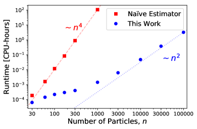
(a)

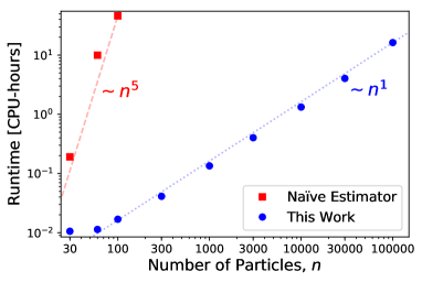
(b)

Figure 3: Timing comparison of the naïve NPCF estimator with that introduced in this work. In the first case, the NPCF is estimated by counting sets of $N$ particles, via (3), weighting by the relevant basis functions (§2). The new estimators exploit hyperspherical harmonic decompositions to reduce the estimator to a sum over pairs. Here, we show results for a variety of choices of $n$, for both 4PCF estimation on the two-sphere (left), and 5PCF estimation in 3D Cartesian space (right). As expected, the runtime of naïve estimator scales as $n^{N}$ (as indicated by the red dotted lines), but the new estimators scale as $n^{2}$ for the 4PCF, or $n$ for the 5PCF. The latter scaling arises since we are dominated by the sum over intermediate momenta $[\boldsymbol{\ell}^{i}]$, rather than the sum over pairs; at larger $n$, we expect a quadratic scaling with $n$. All computations were performed in Julia using 16 CPUs, and we have verified that the measured NPCF components agree to machine precision.

4.1 Cosmic Microwave Background

Cosmic Microwave Background (CMB) radiation encodes a snapshot of the Universe at the epoch of recombination, around $380,000$ years after the Big Bang. This may be probed using microwave satellites such as WMAP and Planck, which map the CMB temperature fluctuations as a function of direction; such observations have been used to place strong constraints on cosmological parameters such as the matter density and Universe’s expansion rate (e.g., 38, 39).

In this setting, the random field in question is the fractional temperature fluctuation on the 2-sphere, $\Theta:\mathbb{S}^{2}\to\mathbb{R}$, i.e. $\mathbb{M}^{D}=\mathbb{S}^{2}$. Conventionally, $\Theta$ is expanded in $D=3$ spherical harmonics as $\Theta(\phi,\theta;\hat{\mathbf{n}})=\sum_{\lambda=0}^{\infty}\sum_{\mu=-\lambda}^{\lambda}\Theta_{\lambda\mu}Y_{\lambda\mu}(\phi,\theta)$, using spherical polar coordinates $\phi\in[0,2\pi)$, $\theta\in[0,\pi)$ relative to some pole on the sphere at position vector $\hat{\mathbf{n}}$. The statistical properties of $\Theta$ are then characterized in terms of the spherical harmonic coefficients $\Theta_{\lambda\mu}$ (often denoted $a_{\lambda\mu}^{T}$). To apply the techniques of this work, we instead expand the temperature fluctuations using the $D=2$ hyperspherical harmonics (§11.2), i.e.

$$\Theta(\mathbf{r};\hat{\mathbf{n}})=\sum_{\ell=0}^{\infty}\Theta_{\ell}(\theta)Y_{\ell}(\phi)\equiv\frac{1}{\sqrt{2\pi}}\sum_{\ell=0}^{\infty}\Theta_{\ell}(\theta)e^{i\ell\phi},$$ (41)

identifying $\ell$ as the total angular momentum and $\theta$ as the radial coordinate relative to $\hat{\mathbf{n}}$, which acts as an origin on $\mathbb{S}^{2}$. This is a convenient basis for computing higher-order clustering statistics on the two-sphere, since (a) it avoids the need for an embedding space, and (b), it provides a natural split into isotropic and anisotropic correlators.

As in (1), the temperature NPCF is defined as a statistical average over $\Theta$:

$$\zeta(\mathbf{r}^{1},\ldots,\mathbf{r}^{N-1})=\mathbb{E}_{\Theta}\left[\Theta(\mathbf{0};\hat{\mathbf{n}})\Theta(\mathbf{r}^{1};\hat{\mathbf{n}})\cdots\Theta(\mathbf{r}^{N-1};\hat{\mathbf{n}})\right];$$ (42)

by statistical homogeneity, this is independent of the choice of origin $\hat{\mathbf{n}}$. (42) may be expanded in the basis of (25), where the $D=2$ basis functions take the form

$$\mathcal{P}^{L}_{\ell^{1}\ldots\ell^{N-1}}(\phi^{1},\ldots,\phi^{N-1}) = (2\pi)^{-(N-1)/2}\mathrm{exp}\left[i(\ell^{1}\phi^{1}+\cdots+\ell^{N-1}\phi^{N-1})\right],$$ (43)

with $\ell^{1}+\cdots+\ell^{N-1}=L$, where $L=0$ for isotropic correlators. Note that no intermediate angular momenta need to be specified due to the coupling rules of (20). As in (34), we may form an $\mathcal{O}(n^{2})$ estimator for the NPCF coefficients:

$$\zeta_{\ell^{1}\ldots\ell^{N-1}}^{L}(\theta^{1},\ldots,\theta^{N-1}) = \frac{1}{4\pi}\int_{\mathbb{S}^{2}}d\Omega_{2}\,\left[\Theta(\hat{\mathbf{n}})a_{\ell^{1}}(\hat{\mathbf{n}};\theta^{1})\cdots a_{\ell^{N-1}}(\hat{\mathbf{n}};\theta^{N-1})\right],$$ (44)

$$a_{\ell}(\hat{\mathbf{n}};\theta) \equiv \frac{1}{\sqrt{2\pi}}\int_{0}^{2\pi}d\phi\,\Theta(\phi,\theta;\hat{\mathbf{n}})e^{i\ell\phi}.$$

The first integral is over all possible choices of origin $\hat{\mathbf{n}}$, whilst the second is over a circle centered at $\hat{\mathbf{n}}$ with radial parameter $\theta$ (which may be discretized into bins, as before).

Such estimators are straightforward to implement and allow efficient computation of the higher-order CMB NPCFs, albeit in a basis somewhat different to that usually adopted. We caution that the $\ell$ indices play a different role to those of the $\lambda$ indices appearing in the standard spherical harmonic expansion of $\Theta$. In our basis, $\ell$ represents angular momentum around an origin on the 2-sphere, whilst $\lambda$ is with reference to the origin of the 2-sphere in the embedding space $\mathbb{R}^{3}$. In practice, this allows us to restrict to much smaller $\ell$ than used conventionally. We further note that the CMB contains also polarization fluctuations. These may be analyzed using an extension of the above formalism, replacing the hyperspherical harmonics with spin-weighted hyperspherical harmonics (e.g., 40, 41).

To give a sense of how the above algorithms work in CMB contexts, we consider a simple problem: estimating the isotropic 4PCF of randomly placed points on the two-sphere. This corresponds to the above scenarios with $N=4$, $D=2$ and a spherical geometry. For this test, we generate a set of $n$ evenly distributed points, and compute the coefficients $\zeta_{\ell^{1}\ell^{2}\ell^{3}}^{0,b^{1}b^{2}b^{3}}$, using $10$ radial bins per dimension with $\cos\theta\in[-0.5,0.5)$ and $\ell_{\rm max}=4$. This leads to a total of $35$ ($120$) angular (radial) components. Timing results for the computation using both the naïve and quadratic estimators (projecting the 4PCF onto the same basis functions in both cases) are shown in Fig. 3(a) for a variety of choices of $n$, using our public Julia code. As expected, the runtime scales as $n^{4}$ for the naïve estimator, which leads to unwieldy computation times even for a few thousand particles. For the estimators introduced in this work, the runtime scales as $n^{2}$ for large $n$, as expected from the algorithm’s complexity.

4.2 Hydrodynamic Turbulence

NPCFs have found significant use in the study of hydrodynamical turbulence. Being a chaotic process, the evolution of the velocity and density fields in a turbulent flow cannot be treated deterministically; rather, they must be analyzed statistically. Furthermore, the density fields of turbulent media are known to be close to log-normal (42), implying that the higher-order NPCFs functions contain a wealth of information, particularly concerning the sonic and Alfvénic Mach numbers (e.g., 43, 44, 45, 15).

One of the simplest observables is the turbulent density field, $\rho:\mathbb{R}^{3}\to\mathbb{R}$, whose $N$-point function is defined in (1). In the absence of any external forcing, we expect the NPCF to be statistically isotropic, thus it can be expanded via (28) in terms of the $D=3$ basis functions with $\boldsymbol{L}=\boldsymbol{0}$. As shown in §11.2, the corresponding one-particle basis functions are just the usual spherical harmonics, $Y_{m\ell}(\hat{\mathbf{r}})$, and their coupling can be expressed in terms of Wigner 3-$j$ symbols.

As before, we may form $\mathcal{O}(n^{2})$ estimators for the NPCF coefficients via (34). As an example, the isotropic 5PCF estimator becomes (ignoring radial binning for clarity)

$$\zeta^{\boldsymbol{0}}_{\ell^{1}\ell^{2}\ell^{12}\ell^{3}\ell^{4}}(r^{1},r^{2},r^{3}) = \frac{1}{V_{3}}(-1)^{\ell^{1}+\ell^{2}+\ell^{3}+\ell^{4}}\sum_{m^{1}m^{2}m^{3}m^{4}}(-1)^{\ell^{12}-m^{12}}\sqrt{2\ell^{12}-1}\begin{pmatrix}{\ell^{1}}&{\ell^{2}}&{\ell^{12}}\\ {m^{1}}&{m^{2}}&{-m^{12}}\end{pmatrix}\begin{pmatrix}{\ell^{12}}&{\ell^{3}}&{\ell^{4}}\\ {m^{12}}&{m^{3}}&{m^{4}}\end{pmatrix}$$ (45)

$$\,\times\,\int_{\mathbb{R}^{3}}d\mathbf{s}\,\left[\rho(\mathbf{s})a_{m^{1}\ell^{1}}(\mathbf{s};r^{1})a_{m^{2}\ell^{2}}(\mathbf{s};r^{2})a_{m^{3}\ell^{3}}(\mathbf{s};r^{3})a_{m^{4}\ell^{4}}(\mathbf{s};r^{4})\right],$$

where $V_{3}$ is the volume of the space, $m^{12}\equiv m^{1}+m^{2}$, and $a_{m\ell}(\mathbf{s};r)=\int_{\mathbb{S}^{2}}d\Omega_{2}\,\rho(\mathbf{s}+\mathbf{r})Y^{*}_{m\ell}(\hat{\mathbf{r}})$. Introducing spin-weighted (or vector) spherical harmonics, the approach may be extended to tensorial correlators, such as those of the velocity field.

Fig. 3(b) presents a practical demonstration of the isotropic 5PCF estimator, applied to $n$ discrete points in 3D. We consider ten radial bins in $[0.1,0.4]$ for uniformly distributed data in a periodic cube of length $1$, and fix $\ell_{\rm max}=4$. In this case, the 5PCF is specified by four radial bin indices and five angular multiplets, as in (45). This gives a total of $210$ radial and $585$ angular components. As before, we find that the runtime of the naïve estimator scales as $n^{N}$, which quickly becomes computationally prohibitive. For the NPCF estimator of this work, the runtime appears to be linear in $n$, rather than quadratic: this occurs since the work is dominated by the $m^{i}$ summations (cf. §33.2), though we expect the $n^{2}$ scaling to dominate for denser samples. In all cases however, our approach is significantly faster than that of the naïve estimator. We note that our algorithm can be further accelerated by gridding the data, and making use of Fourier transforms.

4.3 Large-Scale Structure

The large-scale distribution of matter in the late Universe follows a weakly non-Gaussian distribution and is commonly analyzed using $N$-point statistics (e.g., 46). The underlying space is expected to be flat, homogeneous, and isotropic, and is thus described by the metric of (6) with $k=0$ and $D=3$. A common task in cosmology is the estimation of isotropic NPCFs for the galaxy overdensity field, $\delta_{g}:\mathbb{R}^{3}\to\mathbb{R}$; this proceeds identically to §44.2, except that the data are discrete. Full discussion of this (including implementation in the encore code) is presented in our companion work (16), and allows information to be extracted from the high-order NPCFs, which are otherwise computationally prohibitive to measure.

Due to the effects of redshift-space distortions (e.g., 47), observed galaxy distributions are not isotropic, implying that the decomposition of (28) does not capture all possible NPCF information. However, the statistics are invariant under rotations about an (assumed fixed) line-of-sight, here set to $\hat{\mathbf{x}}^{3}$. For a full treatment, we must instead expand the NPCF using Eq. 25, keeping only terms with $L_{1}=0$ (cf. §22.3):

$$\zeta(\mathbf{r}^{1},\ldots,\mathbf{r}^{N-1})=\sum_{L=0}^{\infty}\sum_{{\boldsymbol{\Lambda}}}\zeta_{\boldsymbol{\Lambda}}^{0L}(r^{1},\ldots,r^{N-1})\mathcal{P}^{0L}_{{\boldsymbol{\Lambda}}}(\hat{\mathbf{r}}^{1},\ldots,\hat{\mathbf{r}}^{N-1}),$$ (46)

writing $L\equiv L_{2}$. As an example, the 3PCF becomes

$$\zeta(\mathbf{r}^{1},\mathbf{r}^{2}) = \sum_{L=0}^{\infty}\sum_{\ell^{1}\ell^{2}}\zeta^{0L}_{\ell^{1}\ell^{2}}(r^{1},r^{2})\mathcal{P}^{0L}_{\ell^{1}\ell^{2}}(\hat{\mathbf{r}}^{1},\hat{\mathbf{r}}^{2}),$$ (47)

$$\mathcal{P}^{0L}_{\ell^{1}\ell^{2}}(\hat{\mathbf{r}}^{1},\hat{\mathbf{r}}^{2}) = (-1)^{\ell^{2}-\ell^{1}}\sqrt{2L+1}\sum_{m}\begin{pmatrix}{\ell^{1}}&{\ell^{2}}&{L}\\ {m}&{-m}&{0}\end{pmatrix}Y_{\ell^{1}m}(\hat{\mathbf{r}}^{1})Y_{\ell^{2}-m}(\hat{\mathbf{r}}^{2}).$$

(cf.  48, 49). Such statistics may be estimated via (34), as before. The above decomposition provides a complete basis for the redshift-space 3PCF (analogous to 49) and extends naturally to higher orders, which have not previously been discussed.

5 Summary

Many areas of research require computation of clustering statistics from continuous or discrete random fields. Perhaps the most prevalent statistic is the $N$-point correlation function (NPCF), defined as the statistical average over $N$ fields in different spatial locations. If the random field is Gaussian-distributed, only the 2PCF is of interest; in the general case, all correlators have non-trivial forms. Given a set of $n$ particles, a naïve estimator for the NPCF components in some basis has $\mathcal{O}(n^{N})$ complexity with respect to $n$. As $N$ increases, this rapidly becomes computationally infeasible to apply: alternative methods must be sought if one wishes to unlock the information contained within higher-order NPCFs.

This work considers NPCF estimation on isotropic and homogeneous manifolds in $D$ dimensions. Under these assumptions (which encompass spherical, flat, and hyperbolic geometries), we show that any function of one position can be expanded in hyperspherical harmonics; a $D$-dimensional analog of the conventional spherical harmonics. These are also eigenstates of the angular momentum operators; utilizing the mathematics of angular momentum addition, we can construct basis functions involving $(N-1)$ points on $\mathbb{S}^{D-1}$ as a sum over products of $(N-1)$ hyperspherical harmonics. This forms a natural angular basis for the NPCF, particularly if the random field is statistically isotropic. The decomposition allows construction of an NPCF estimator that separates into a product of $(N-1)$ spatial integrals; this has $\mathcal{O}(n^{2})$ complexity (with respect to $n$), or $\mathcal{O}(n_{\rm g}\log n_{\rm g})$ using FFTs with $n_{\rm g}$ grid-points. The algorithms have been validated numerically using a new Julia implementation; in all scenarios tested, we find our approach to yield significantly faster measurements of the NPCF coefficients in our angular momentum basis.

Such techniques will allow high-order correlation functions to be computed from data, allowing more complete analysis of phenomena ranging from fluid turbulence to galaxy clustering. Furthermore, since the algorithm can be applied to scenarios with $D\neq 3$, we may consider also the computation of NPCFs on the surface of spheres (relevant e.g., for atmospheric physics), or in higher-dimensional atomic treatments with $D=6$ (e.g., 19). These ideas may be extended further; a case of particular interest is in the correlation functions of random fields with non-zero spin; these are required to describe the statistics of tensor fields such as turbulent velocities and CMB polarization.

We thank David Spergel for encouraging us to write this paper, as well as Robert Cahn, Simone Ferraro, Jiamin Hou, Bhuv Jain, Adam Lidz, Moritz Münchmeyer, Shivam Pandey, Ue-Li Pen, Cristiano Sabiu, Frederik Simons, Sauro Succi, and Wen Yan for insightful discussions. We are additionally indebted to the anonymous referees for insightful feedback. OP acknowledges funding from the WFIRST program through NNG26PJ30C and NNN12AA01C and thanks the Simons Foundation for additional support.

Appendix A Hyperspherical Harmonics

The hyperspherical harmonics are defined by the eigenfunction equation (8), which can be written explicitly as

$$\Delta_{\mathbb{S}^{D-1}}Y(\hat{\mathbf{r}})\equiv\sin^{2-D}\theta_{1}\,\partial_{\theta_{1}}\left[\sin^{D-2}\theta_{1}\,\partial_{\theta_{1}}Y(\hat{\mathbf{r}})\right]+\cdots+\sin^{-2}\theta_{1}\cdots\sin^{-2}\theta_{D-2}\,\partial_{\theta_{D-1}}^{2}Y(\hat{\mathbf{r}}) = -\lambda_{D-1}Y(\hat{\mathbf{r}})$$ (48)

in hyperspherical coordinates. Importantly, the Laplace-Beltrami operator on the $K$-sphere may be written in terms of that on the $(K-1)$-sphere, allowing us to compute the angular basis functions iteratively, first solving for the 1-sphere basis, which can then be used to find the solution on the 2-sphere, et cetera. This leads to the hierarchy $Y^{(K)}(\theta_{1},\ldots,\theta_{K})=\Theta_{K}(\theta_{K})Y^{(K-1)}(\theta_{1},\ldots,\theta_{K-1})$, where

$$\sin^{1-K}\theta_{K}\,\frac{\partial}{\partial\theta_{K}}\left[\sin^{K-1}\theta_{K}\,\frac{\partial\Theta_{K}(\theta_{K})}{\partial\theta_{K}}\right]-\lambda_{K-1}\sin^{-2}\theta_{K}\,\Theta_{K}(\theta_{K})=-\lambda_{K}\Theta_{K}(\theta_{K})$$ (49)

(23), writing the eigenvalue for the $K$-sphere as $\lambda_{K}$. Starting from the 1-sphere basis functions $\Theta_{1}(\theta_{1})=(2\pi)^{-1/2}\mathrm{exp}\left(-i\ell_{1}\theta_{1}\right)$, we can form the full hyperspherical harmonics by solving (49), giving $Y_{\ell_{1}\ldots\ell_{D-1}}(\theta_{1},\ldots,\theta_{D-1})\equiv\Theta_{1}(\theta_{1})\Theta_{2}(\theta_{2})\cdots\Theta_{D-1}(\theta_{D-1})$, with

$$Y_{\ell_{1}\ldots\ell_{D-1}}(\theta_{1},\ldots,\theta_{D-1}) \equiv \Theta_{1}(\theta_{1})\Theta_{2}(\theta_{2})\cdots\Theta_{D-1}(\theta_{D-1}),$$ (50)

$$\Theta_{K}(\theta_{K}) = \sqrt{\frac{2\ell_{K}+K-1}{2}\frac{(\ell_{K}+\ell_{K-1}+K-2)!}{(\ell_{K}-\ell_{K-1})!}}\sin^{1-K/2}\theta_{K}\,P_{\ell_{K}+K/2-1}^{-(\ell_{K-1}+K/2-1)}\left(\cos\theta_{K}\right),\quad(2\leq K\leq D-1),$$

where $P_{L}^{M}(x)$ is an associated Legendre polynomial (e.g., 34, §14.3). The indices $\ell_{i}$ are related to the Laplace-Beltrami eigenvalues of (7) via $\lambda_{K}=\ell_{K}(\ell_{K}+K-1)$ and must satisfy the selection rules of (9).

Under complex conjugation and parity transformations, the hyperspherical harmonics transform as

$$Y_{\ell_{1}\ell_{2}\ldots\ell_{D-1}}^{*}(\hat{\mathbf{r}})=(-1)^{\ell_{1}}Y_{(-\ell_{1})\ell_{2}\ldots\ell_{D-1}}(\hat{\mathbf{r}}),\qquad\mathbb{P}\left[Y_{\ell_{1}\ldots\ell_{D-1}}(\hat{\mathbf{r}})\right]=(-1)^{\ell_{D-1}}Y_{\ell_{1}\ldots\ell_{D-1}}(\hat{\mathbf{r}}),$$ (51)

where the parity operator, $\mathbb{P}$, sends $\mathbf{r}\to-\mathbf{r}$ and thus $\theta_{1}\to\pi+\theta_{1}$, $\theta_{k}\to\pi-\theta_{k}$ for $k>1$. The latter equation can be verified by noting that the action of the parity operator on the basis components of (50) are $\mathbb{P}[\Theta_{1}(\theta_{1})]=(-1)^{\ell_{1}}\Theta_{1}(\theta_{1})$ and $\mathbb{P}[\Theta_{K}(\theta_{K})]=(-1)^{\ell_{K}-\ell_{K-1}}$ for $K>1$.

References

• (1) S Garrett-Roe, P Hamm, Three-point frequency fluctuation correlation functions of the oh stretch in liquid water. \JournalTitleThe Journal of Chemical Physics 128, 104507 (2008).
• (2) JG Berryman, Interpolating and integrating three-point correlation functions on a lattice. \JournalTitleJournal of Computational Physics 75, 86–102 (1988).
• (3) VS DOTSENKO, Three-point correlation functions of the minimal conformal theories coupled to 2d gravity. \JournalTitleModern Physics Letters A 06, 3601–3612 (1991).
• (4) K Hwang, B Schmittmann, RKP Zia, Three-point correlation functions in uniformly and randomly driven diffusive systems. \JournalTitlePhys. Rev. E 48, 800–809 (1993).
• (5) F Šanda, S Mukamel, Multipoint correlation functions for continuous-time random walk models of anomalous diffusion. \JournalTitlePhysical Review E 72, 031108 (2005).
• (6) AW Moore, et al., Fast Algorithms and Efficient Statistics: N-Point Correlation Functions in Mining the Sky, eds. AJ Banday, S Zaroubi, M Bartelmann. p. 71 (2001).
• (7) PJE Peebles, Large Scale Clustering in the Universe in Large Scale Structures in the Universe, eds. MS Longair, J Einasto. Vol. 79, p. 217 (1978).
• (8) S Alam, et al., Testing the theory of gravity with DESI: estimators, predictions and simulation requirements. \JournalTitlearXiv e-prints, arXiv:2011.05771 (2020).
• (9) LL Zhang, UL Pen, Fast n-point correlation functions and three-point lensing application. \JournalTitleNew Astronomy 10, 569–590 (2005).
• (10) CG Sabiu, B Hoyle, J Kim, XD Li, Graph Database Solution for Higher-order Spatial Statistics in the Era of Big Data. \JournalTitleAstrophysical Journal Supplement 242, 29 (2019).
• (11) Z Slepian, DJ Eisenstein, Computing the three-point correlation function of galaxies in O(N2̂) time. \JournalTitleMonthly Notices of the Royal Astronomical Society 454, 4142–4158 (2015).
• (12) I Szapudi, Three-Point Statistics from a New Perspective. \JournalTitleAstrophysical Journal Letters 605, L89–L92 (2004).
• (13) Z Slepian, et al., Detection of baryon acoustic oscillation features in the large-scale three-point correlation function of SDSS BOSS DR12 CMASS galaxies. \JournalTitleMonthly Notices of the Royal Astronomical Society 469, 1738–1751 (2017).
• (14) Z Slepian, et al., The large-scale three-point correlation function of the SDSS BOSS DR12 CMASS galaxies. \JournalTitleMonthly Notices of the Royal Astronomical Society 468, 1070–1083 (2017).
• (15) SKN Portillo, Z Slepian, B Burkhart, S Kahraman, DP Finkbeiner, Developing the 3-point Correlation Function for the Turbulent Interstellar Medium. \JournalTitleAstrophysical Journal 862, 119 (2018).
• (16) OHE Philcox, et al., ENCORE: Estimating Galaxy $N$-point Correlation Functions in $\mathcal{O}(N_{\rm g}^{2})$ Time. \JournalTitlearXiv e-prints, arXiv:2105.08722 (2021).
• (17) S Chatterjee, B Bhui, Homogeneous Cosmological Model in Higher Dimension. \JournalTitleMonthly Notices of the Royal Astronomical Society 247, 57 (1990).
• (18) RM Wald, General relativity. (1984).
• (19) JW Cooper, U Fano, F Prats, Classification of two-electron excitation levels of helium. \JournalTitlePhys. Rev. Lett. 10, 518–521 (1963).
• (20) H Cohl, Fundamental solution of laplace’s equation in hyperspherical geometry. \JournalTitleSymmetry, Integrability and Geometry: Methods and Applications (2011).
• (21) C Frye, CJ Efthimiou, Spherical Harmonics in p Dimensions. \JournalTitlearXiv e-prints, arXiv:1205.3548 (2012).
• (22) JD Louck, Theory of angular momentum in n-dimensional space. \JournalTitleTechnical Report (1960).
• (23) A Higuchi, Symmetric tensor spherical harmonics on the n-sphere and their application to the de sitter group so(n,1). \JournalTitleJournal of Mathematical Physics 28, 1553–1566 (1987).
• (24) A Tichai, R Wirth, J Ripoche, T Duguet, Symmetry reduction of tensor networks in many-body theory I. Automated symbolic evaluation of $SU(2)$ algebra. \JournalTitlearXiv e-prints, arXiv:2002.05011 (2020).
• (25) LC Biedenharn, JD Louck, PA Carruthers, Angular Momentum in Quantum Physics: Theory and Application, Encyclopedia of Mathematics and its Applications. (Cambridge University Press), (1984).
• (26) DA Varshalovich, AN Moskalev, VK Khersonskii, Quantum Theory of Angular Momentum. (1988).
• (27) S Szalay, et al., Tensor product methods and entanglement optimization for ab initio quantum chemistry. \JournalTitlearXiv e-prints, arXiv:1412.5829 (2014).
• (28) A Tichai, R Schutski, GE Scuseria, T Duguet, Tensor-decomposition techniques for ab initio nuclear structure calculations: From chiral nuclear potentials to ground-state energies. \JournalTitlePhysical Review C 99, 034320 (2019).
• (29) P Van Isacker, O(4) Symmetry and Angular Momentum Theory in Four Dimensions, eds. B Gruber, LC Biedenharn, HD Doebner. (Springer US, Boston, MA), pp. 323–340 (1991).
• (30) LC Biedenharn, Wigner coefficients for the r4 group and some applications. \JournalTitleJournal of Mathematical Physics 2, 433–441 (1961).
• (31) J Louck, Angular Momentum Theory, ed. G Drake. (Springer New York, New York, NY), pp. 9–74 (2006).
• (32) MA Caprio, KD Sviratcheva, AE McCoy, Racah’s method for general subalgebra chains: Coupling coefficients of SO(5) in canonical and physical bases. \JournalTitleJournal of Mathematical Physics 51, 093518–093518 (2010).
• (33) G Racah, Group theory and spectroscopy, ed. G Höhler. (Springer Berlin Heidelberg, Berlin, Heidelberg), pp. 28–84 (1965).
• (34) NIST Digital Library of Mathematical Functions (http://dlmf.nist.gov/, Release 1.1.2 of 2021-06-15) (2021) F. W. J. Olver, A. B. Olde Daalhuis, D. W. Lozier, B. I. Schneider, R. F. Boisvert, C. W. Clark, B. R. Miller, B. V. Saunders, H. S. Cohl, and M. A. McClain, eds.
• (35) AV Meremianin, Multipole expansions in four-dimensional hyperspherical harmonics. \JournalTitleJournal of Physics A Mathematical General 39, 3099–3112 (2006).
• (36) RN Cahn, Z Slepian, Isotropic N-Point Basis Functions and Their Properties. \JournalTitlearXiv e-prints, arXiv:2010.14418 (2020).
• (37) A Dutt, V Rokhlin, Fast fourier transforms for nonequispaced data. \JournalTitleSIAM J. Sci. Comput. 14, 1368–1393 (1993).
• (38) E Komatsu, et al., Seven-year Wilkinson Microwave Anisotropy Probe (WMAP) Observations: Cosmological Interpretation. \JournalTitleAstrophysical Journal Supplement 192, 18 (2011).
• (39) Planck Collaboration, et al., Planck 2018 results. VI. Cosmological parameters. \JournalTitleAstronomy and Astrophysics 641, A6 (2020).
• (40) L Dai, M Kamionkowski, D Jeong, Total angular momentum waves for scalar, vector, and tensor fields. \JournalTitlePhysical Review D 86, 125013 (2012).
• (41) M Boyle, How should spin-weighted spherical functions be defined? \JournalTitleJournal of Mathematical Physics 57, 092504 (2016).
• (42) E Vazquez-Semadeni, Hierarchical Structure in Nearly Pressureless Flows as a Consequence of Self-similar Statistics. \JournalTitleAstrophysical Journal 423, 681 (1994).
• (43) G Kowal, A Lazarian, A Beresnyak, Density Fluctuations in MHD Turbulence: Spectra, Intermittency, and Topology. \JournalTitleAstrophysical Journal 658, 423–445 (2007).
• (44) B Burkhart, D Falceta-Gonçalves, G Kowal, A Lazarian, Density Studies of MHD Interstellar Turbulence: Statistical Moments, Correlations and Bispectrum. \JournalTitleAstrophysical Journal 693, 250–266 (2009).
• (45) B Burkhart, S Stanimirović, A Lazarian, G Kowal, Characterizing Magnetohydrodynamic Turbulence in the Small Magellanic Cloud. \JournalTitleAstrophysical Journal 708, 1204–1220 (2010).
• (46) PJE Peebles, The Galaxy and Mass N-Point Correlation Functions: a Blast from the Past in Historical Development of Modern Cosmology, Astronomical Society of the Pacific Conference Series, eds. VJ Martínez, V Trimble, MJ Pons-Bordería. Vol. 252, p. 201 (2001).
• (47) N Kaiser, Clustering in real space and in redshift space. \JournalTitleMonthly Notices of the Royal Astronomical Society 227, 1–21 (1987).
• (48) Z Slepian, DJ Eisenstein, A practical computational method for the anisotropic redshift-space three-point correlation function. \JournalTitleMonthly Notices of the Royal Astronomical Society 478, 1468–1483 (2018).
• (49) NS Sugiyama, S Saito, F Beutler, HJ Seo, A complete FFT-based decomposition formalism for the redshift-space bispectrum. \JournalTitleMonthly Notices of the Royal Astronomical Society 484, 364–384 (2019).