Riemannian Convex Potential Maps

Riemannian Convex Potential Maps: Supplementary Material

Abstract

Modeling distributions on Riemannian manifolds is a crucial component in understanding non-Euclidean data that arises, e.g., in physics and geology. The budding approaches in this space are limited by representational and computational tradeoffs. We propose and study a class of flows that uses convex potentials from Riemannian optimal transport. These are universal and can model distributions on any compact Riemannian manifold without requiring domain knowledge of the manifold to be integrated into the architecture. We demonstrate that these flows can model standard distributions on spheres, and tori, on synthetic and geological data. Our source code is freely available online at github.com/facebookresearch/rcpm.

1 Introduction

Today’s generative models have had wide-ranging successes of modeling non-trivial probability distributions that naturally arise in fields such as physics (Köhler et al., 2019; Rezende et al., 2019), climate science (Mathieu & Nickel, 2020), and reinforcement learning (Haarnoja et al., 2018). Generative modeling on “straight” spaces (i.e., Euclidean) are pretty well-developed and include (continuous) normalizing flows (Rezende & Mohamed, 2015; Dinh et al., 2016; Chen et al., 2018), generative adversarial networks (Goodfellow et al., 2014), and variational auto-encoders (Kingma & Welling, 2014; Rezende et al., 2014).

In many applications however, data resides on spaces with more complicated structure, e.g., Riemannian manifolds such as spheres, tori, and cylinders. Using Euclidean generative models on this data is problematic from two aspects: first, Euclidean models will allocate mass in “infeasible” areas of the space; and second, Euclidean models will often need to squeeze mass in zero volume subspaces. Moreover, knowledge of the space geometry can improve the learning process by incorporating an efficient geometric inductive bias as part of the modeling and learning pipeline.

Flow-based generative models are the state-of-the-art in Euclidean settings and are starting to be extended to Riemannian manifolds (Rezende et al., 2020; Mathieu & Nickel, 2020; Lou et al., 2020). However, in contrast with some models in the Euclidean case (Kong & Chaudhuri, 2020; Huang et al., 2020), the representational capacity and universality of these models is not well-understood. Some of these approaches are efficiently tailored to specific choices of manifolds, but the methods and theory of flows on general Riemannian manifolds are not well-understood.

In this paper we introduce the Riemannian Convex Potential Map (RCPM), a generic model for generative modeling on arbitrary Riemannian manifolds that enjoys universal representational power. RCPM (illustrated in fig. 2) is based on Optimal Transport (OT) over Riemannian manifolds (McCann, 2001; Villani, 2008; Sei, 2013; Rezende et al., 2020) and generalizes the convex potential flows in the Euclidean setting by Huang et al. (2020). We prove that RCPMs are universal on any compact Riemannian manifold, which comes from the fact that our discrete $c$-concave potential functions are universal. Our experimental demonstrations show that RCPMs are competitive and model standard distributions on spheres and tori. We further show a case study in modeling continental drift where we transport Earth’s land mass on the sphere.

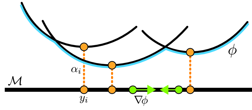
Figure 1: Illustration of a discrete $c$-concave function $\phi$ (blue) over a base manifold ${\mathcal{M}}$ (bold line). These consist of discrete components $\{\alpha_{i},y_{i}\}$ and have a Riemannian gradient $\nabla\phi\in T_{x}{\mathcal{M}}$.

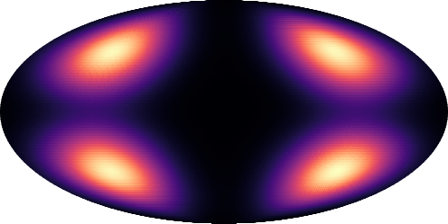
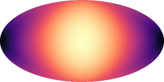
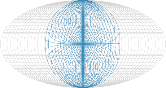
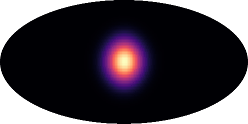
Figure 2: Illustration of a Riemannian convex potential map on a sphere. From left to right: 1) base distribution $\mu$ of a mixture of wrapped Gaussians, 2) learned $c$-convex potential, 3) mesh grid distorted by the exponential map of the Riemannian gradient of the potential, 4) transformed distribution $\nu$.

2 Related Work

Euclidean potential flows.

Most related to our work, is the work by Huang et al. (2020) that leveraged Euclidean optimal transport, parameterized using input convex neural networks (ICNNs) (Amos et al., 2017) to construct universal normalizing flows on Euclidean spaces. Similarly, Korotin et al. (2021); Makkuva et al. (2020) compute optimal transport maps via ICNNs. Riemannian optimal transport replaces the standard Euclidean convex functions with so-called $c$-convex or $c$-concave functions, and the Euclidean translation by exponential map. Unfortunately, the notion of $c$-convex or $c$-concave functions is intricate and a simple characterization of such functions is not known. Our approach is to approximate arbitrary $c$-concave functions on general Riemannian manifolds using discrete $c$-concave functions that are simply the minimum of a finite number of translated squared intrinsic distance functions, see fig. 1. Intuitively, this construction resembles the approximation of a Euclidean concave function as the minimum of a finite collection of affine tangents. Although simple, we prove that discrete $c$-concave functions are in fact dense in the space of $c$-concave functions and therefore replacing general $c$-concave functions with discrete $c$-concave functions leads to a universal Riemannian OT model. Related, Gangbo & McCann (1996) considered OT maps of discrete measures which are defined via discrete $c$-concave functions.

Exponential map flows.

Sei (2013); Rezende et al. (2020) propose distinct parameterizations for $c$-convex functions living on the sphere specifically. The latter applies it to training flows on the sphere using the construction from McCann’s theorem. Our work can be seen as a generalization of the exponential-map approach in Rezende et al. (2020) to arbitrary Riemannian manifolds. In contrast to this work, the maps from our discrete $c$-concave layers are universal.

Other Riemannian flows.

Mathieu & Nickel (2020); Lou et al. (2020) propose extensions of continuous normalizing flows to the Riemannian manifold setting. These are flexible with respect to the choice of manifold, but their representational capacity is not well-understood and solving ODEs on manifolds can be expensive. In parallel, Brehmer & Cranmer (2020) proposed a method for simultaneously learning the manifold data lives on and a normalizing flow on the learned manifold. Bose et al. (2020) consider hyperbolic normalizing flows.

Optimal transport on Riemannian manifolds.

Optimal transport on spherical manifolds has been extensively studied from theoretical standpoints. Figalli & Rifford (2009); Loeper (2009); Kim & McCann (2012) study the regularity (continuity, smoothness) of transport maps on spheres and other non-negatively curved manifolds. Regularity and smoothness are more intricate on negatively curved manifolds, e.g. hyperbolic spaces. Nevertheless, several works demonstrated that transport can be made smooth through a minor change to the Riemannian cost (Lee & Li, 2012). Alvarez-Melis et al. (2020); Hoyos-Idrobo (2020) leverage this to learn transport maps on hyperbolic spaces, in which case maps are parameterized as hyperbolic neural networks.

3 Background

In this section, we introduce the relevant background on normalizing flows and Riemannian optimal transport theory.

3.1 Normalizing flows

Normalizing flows parameterize probability distributions $\nu\in{\mathcal{P}}({\mathcal{M}})$, on a manifold ${\mathcal{M}}$, by pushing a simple base (prior) distribution $\mu\in{\mathcal{P}}({\mathcal{M}})$ through a diffeomorphism $s:{\mathcal{M}}\rightarrow{\mathcal{M}}$.

In turn, sampling from distribution $\nu$ amounts to transforming samples $x$ taken from the base distribution via $s$:

$$y=s(x)\sim\nu,\quad\text{where }x\sim\mu.$$ (1)

In the language of measures, $\nu$ is the push-forward of the base measure $\mu$ through the transformation $s$, denoted by $\nu=s_{\#}\mu$. If densities exist, then they adhere the change of variables formula

$$\nu(y)=\mu(x)|\det J_{s}(x)|^{-1},$$ (2)

where we slightly abuse notation by denoting the densities again as $\mu,\nu$. In practice, a normalizing flow $s$ is often defined as a composition of simpler, primitive diffeomorphisms $s_{1},\ldots,s_{T}:{\mathcal{M}}\rightarrow{\mathcal{M}}$, i.e.,

$$s=s_{T}\circ\cdots\circ s_{1}.$$ (3)

For a more substantial review of computational and representational trade-offs inherent to this class of model on Euclidean spaces, we refer to Papamakarios et al. (2019).

3.2 $c$-convexity and concavity

Let $({\mathcal{M}},g)$ be a smooth compact Riemannian manifold without boundary, and $c(x,y)=\frac{1}{2}d(x,y)^{2}$, where $d(x,y)$ is the intrinsic distance function on the manifold. We use the following generalizations of convex and concave functions:

Definition 1.

A function $\phi:{\mathcal{M}}\rightarrow\mathbb{R}\cup\left\{+\infty\right\}$ is $c$-convex if it is not identically $+\infty$ and there exists $\psi:{\mathcal{M}}\rightarrow\mathbb{R}\cup\left\{\pm\infty\right\}$ such that

$$\phi(x)=\sup_{y\in{\mathcal{M}}}\left(-c(x,y)+\psi(y)\right)$$ (4)

Definition 2.

A function $\phi:{\mathcal{M}}\rightarrow\mathbb{R}\cup\left\{-\infty\right\}$ is $c$-concave if it is not identically $-\infty$ and there exists $\psi:{\mathcal{M}}\rightarrow\mathbb{R}\cup\left\{\pm\infty\right\}$ such that

$$\phi(x)=\inf_{y\in{\mathcal{M}}}\left(c(x,y)+\psi(y)\right)$$ (5)

We denote the space of $c$-concave functions on ${\mathcal{M}}$ as $\widehat{{\mathcal{C}}}({\mathcal{M}})$. We also note that if $\psi$ is $c$-concave, $-\psi$ is $c$-convex, hence c-concavity results can be directly extended into c-convexity results by negation. We also use the $c$-infimal convolution:

$$\psi^{c}(y)=\inf_{x\in{\mathcal{M}}}\left(c(x,y)-\psi(x)\right).$$ (6)

$c$-concave functions $\phi$ satisfy the involution property:

$$\phi^{cc}=\phi.$$ (7)

When ${\mathcal{M}}$ is a product of spheres or a Euclidean space, (e.g., spheres, tori), $\widehat{{\mathcal{C}}}({\mathcal{M}})$ is a convex space (Figalli et al., 2010b; Figalli & Villani, 2011) where a convex combinations of $c$-concave functions are $c$-concave. In the case ${\mathcal{M}}=\mathbb{R}^{d}$ and $c(x,y)=-x^{T}y$, Euclidean concavity is recovered.

3.3 Riemannian Optimal Transport

Optimal transport deals with finding efficient ways to push a base probability measure $\mu\in{\mathcal{P}}({\mathcal{M}})$ to a target measure $\nu\in{\mathcal{P}}({\mathcal{M}})$, i.e., $s_{\#}\mu=\nu$. Often $s$ considered is more general than a diffeormorphism, namely a transport plan which is a bi-measure on ${\mathcal{M}}\times{\mathcal{M}}$.

When ${\mathcal{M}}$ is a smooth compact manifold with no boundary, $\mu,\nu\in{\mathcal{P}}({\mathcal{M}})$, and $\mu$ has density (i.e., is absolutely continuous w.r.t. the volume measure of ${\mathcal{M}}$), Theorem 9 of McCann (2001) shows that there is a unique (up-to $\mu$-zero sets) transport map $t:{\mathcal{M}}\rightarrow{\mathcal{M}}$ that pushes $\mu$ to $\nu$, i.e., $s_{\#}\mu=\nu$, and minimizes the transport cost

$$C(s)=\int_{\mathcal{M}}c(x,s(x))d\mu(x).$$ (8)

Furthermore, this OT map is given by

$$t(x)=\exp_{x}\left[-\nabla\phi(x)\right],$$ (9)

where $\phi$ is a $c$-concave function, $\exp$ is the Riemannian exponential map, and $\nabla$ is the Riemannian gradient. Note that equivalently $t(x)=\exp_{x}\left[\nabla\psi(x)\right]$ for $c$-convex $\psi$.

As a consequence, there always exists a (Borel) mapping $t:{\mathcal{M}}\rightarrow{\mathcal{M}}$ such that $t_{\#}\mu=\nu$ where $t$ is of the form of eq. 9. The issue of regularity and smoothness of OT maps is a delicate one and has been extensively studied (see, e.g., Villani (2008); Figalli et al. (2010b); Figalli & Villani (2011)); in general, OT maps are not smooth, but can be seen as a natural generalization to normalizing flows, relaxing the smoothness of $s$. Henceforth, we will call OT maps “flows.” In fact, our discrete $c$-concave functions, the gradient of which are shown to approximate general OT maps, define piecewise smooth maps.

Constant-speed geodesics $\eta:[0,1]\rightarrow{\mathcal{M}}$ between a sample $x$ (from $\mu$) and $t(x)$ can also be recovered $\mu$-almost everywhere on the manifold (Figalli & Villani, 2011) as

$$\eta(l)=\exp_{x}\left[-l\nabla\phi(x)\right].$$ (10)

For a geodesic starting at $x_{0}\in{\mathcal{M}}$, $\eta(0)=x_{0}$ and $\eta(1)=t(x_{0})$.

4 Riemannian Convex Potential Maps

Our goal is to represent optimal transport maps on Riemannian manifolds $t:{\mathcal{M}}\rightarrow{\mathcal{M}}$. The key idea is to build upon the theory of McCann (2001) and parameterize the space of optimal transport maps by $c$-concave functions $\phi:{\mathcal{M}}\rightarrow{\mathcal{M}}$, see definition 2. Given a $c$-concave function, the map $t$ is computed via eq. 9. This requires computing the intrinsic gradient of $\phi$ and the exponential map on ${\mathcal{M}}$.

4.1 Discrete $c$-concave functions

Let $\left\{y_{i}\right\}_{i\in[m]}\subset{\mathcal{M}}$ be a set of $m$ discrete points, where $[m]=\left\{1,2,\ldots,m\right\}$, and define the function $\psi$ to be

$$\psi(x)=\begin{cases}\alpha_{i}&\text{if }x=y_{i}\\ +\infty&\text{otherwise}\end{cases}$$ (11)

where $\alpha_{i}\in\mathbb{R}$ are arbitrary. Plugging this choice in definition 2 of $c$-concave functions, we get that

$$\phi(x)=\min_{i\in[m]}\left(c(x,y_{i})+\alpha_{i}\right)$$ (12)

is $c$-concave. We denote the collection of these functions over ${\mathcal{M}}$ by $\widehat{{\mathcal{C}}}^{d}({\mathcal{M}})$. We will use this modeling metaphor for parameterizing $c$-concave functions. Our learnable parameters of a single $c$-concave function $\psi$ will consist of

$$\theta=\left\{(y_{i},\alpha_{i})\right\}_{i\in[m]}\subset{\mathcal{M}}\times\mathbb{R}.$$ (13)

Let $i_{\star}=\operatorname*{arg\,min}_{i\in[m]}\left(c(x,y_{i})+\alpha_{i}\right)$. The discrete $c$-concave function in eq. 12 is differentiable, except where two pieces $c(x,y_{i})+\alpha_{i}$ meet, and if $x$ belongs to the cut locus of $y_{i_{\star}}$ on ${\mathcal{M}}$, which is of volume measure zero (Takashi, 1996). Excluding such cases, the gradient of $\phi$ at $x$ is:

$$\nabla_{x}\phi(x) =\nabla_{x}\big{[}c(x,y_{i_{\star}})+\alpha_{\star}\big{]}$$ (14)

$$=\nabla_{x}c(x,y_{i_{\star}})=-\log_{x}(y_{i_{\star}}),$$

where $\log$ is the logarithmic map on the manifold. See fig. 1 for an illustration of a discrete $c$-concave function. Intuitively, the optimal transport generated by discrete $c$-concave functions is piecewise constant as $\exp_{x}(-\nabla_{x}\phi(x))=\exp_{x}(-(-\log_{x}(y_{i_{\star}})))=y_{i_{\star}}$. This can be seen as generalizing semi-discrete optimal transport (Peyre & Cuturi, 2019), which aims at finding transport maps between continuous and discrete probability measures, to the manifold setting.

Relation to the Euclidean concave case.

In the Euclidean setting, i.e., when ${\mathcal{M}}=\mathbb{R}^{d}$ and $c(x,y)=-x^{T}y$, a Euclidean concave (closed) function $\phi$ can be expressed as

$$\phi(x)=\inf_{y\in\mathbb{R}^{d}}\left(-x^{T}y+\psi(y)\right).$$

Replacing $\mathbb{R}^{d}$ with a finite set of points $y_{i}\in\mathbb{R}^{d}$, $i\in[m]$, leads to the discrete Legendre-Fenchel transform (Lucet, 1997); it basically amounts to approximating the concave function $\phi$ via the minimum of a collection of affine functions. This transform can be shown to converge to $\phi$ under refinement (Lucet, 1997). We next prove convergence of discrete $c$-concave functions to their continuous counterparts.

Expressive power of discrete $c$-concave functions.

Let us show that eq. 12 can approximate arbitrary $c$-concave functions $\phi:{\mathcal{M}}\rightarrow\mathbb{R}\cup\left\{\infty\right\}$ on compact manifolds ${\mathcal{M}}$. We will prove the following theorem:

Theorem 1.

For compact, boundaryless, smooth manifold ${\mathcal{M}}$, we have $\widehat{{\mathcal{C}}}^{d}({\mathcal{M}})$ dense in $\widehat{{\mathcal{C}}}({\mathcal{M}})$.

By dense we mean that for every $\hat{\phi}\in\widehat{{\mathcal{C}}}({\mathcal{M}})$ there exists a sequence $\phi_{\epsilon}\in\widehat{{\mathcal{C}}}^{d}({\mathcal{M}})$, where ${\epsilon}\downarrow 0$, so that for almost all $x\in{\mathcal{M}}$ we have that $\phi_{\epsilon}(x)\rightarrow\hat{\phi}(x)$ and $\nabla_{x}\phi_{\epsilon}(x)\rightarrow\nabla_{x}\hat{\phi}(x)$, as ${\epsilon}\downarrow 0$.

The proof is based on a construction of $\phi_{\epsilon}$ using an ${\epsilon}$-net of ${\mathcal{M}}$. A set of points $\left\{y_{i}\right\}_{i\in[m]}\subset{\mathcal{M}}$ is called ${\epsilon}$-net if ${\mathcal{M}}\subset\cup_{i\in[m]}B(y_{i},{\epsilon})$, where $B(y_{i},{\epsilon})$ is the ${\epsilon}$-radius ball centered at $y_{i}$. Formulated differently, every point $y\in{\mathcal{M}}$ has a point in the net that is at-most ${\epsilon}$ distance away. On compact manifolds, for arbitrary ${\epsilon}>0$, there exists a finite ${\epsilon}$-net $\left\{y_{i}\right\}_{i\in[m]}$. Note that $m\rightarrow\infty$ as ${\epsilon}\downarrow 0$, but it is finite for every particular ${\epsilon}$. Our candidate for approximating $\hat{\phi}$ is:

$$\phi_{\epsilon}(x)=\min_{i\in[m]}\left(c(x,y_{i})-\hat{\phi}^{c}(y_{i})\right),\\$$ (15)

where $\hat{\phi}^{c}$ is the infimal $c$-convolution (see eq. 6) of $\hat{\phi}$. The approximation in eq. 15 is motivated by the involution property (eq. 7). $\hat{\phi}=(\hat{\phi}^{c})^{c}$ and therefore

$$\hat{\phi}(x)=\inf_{y\in{\mathcal{M}}}\left(c(x,y)-\hat{\phi}^{c}(y)\right).$$

Proof.

Let $\hat{\phi}:{\mathcal{M}}\rightarrow\mathbb{R}$ be an arbitrary $c$-concave function over ${\mathcal{M}}$. Let ${\epsilon}\downarrow 0$ denote a sequence of positive numbers converging monotonically to zero. We will show that $\phi_{\epsilon}$ defined in eq. 15 converges uniformly to $\hat{\phi}$ over ${\mathcal{M}}$ and furthermore, that their Riemannian gradients $\nabla\phi_{\epsilon}(x)$ converge pointwise to $\nabla\hat{\phi}(x)$ for almost all $x\in{\mathcal{M}}$ (i.e., up to a set of zero volume).

Uniform convergence.

We start by noting that $\hat{\phi}^{c}$ is also $c$-concave by definition, and Lemma 2 in McCann (2001) implies that $\hat{\phi}^{c}$ is $|{\mathcal{M}}|$-Lipschitz, namely

$$\left|\hat{\phi}^{c}(x)-\hat{\phi}^{c}(y)\right|\leq|{\mathcal{M}}|d(x,y),$$

for all $x,y\in{\mathcal{M}}$. We denote by $|{\mathcal{M}}|$ the diameter of ${\mathcal{M}}$, that is:

$$\left|{\mathcal{M}}\right|=\sup_{x,y\in{\mathcal{M}}}d(x,y),$$ (16)

and $|{\mathcal{M}}|<\infty$ since ${\mathcal{M}}$ is compact. In particular $\hat{\phi}^{c}$ is either everywhere infinite (non-interesting case), or is finite (in fact, bounded) over ${\mathcal{M}}$.

Next, we establish an upper bound. For all $x\in{\mathcal{M}}$:

$$\hat{\phi}(x) =\inf_{y\in{\mathcal{M}}}\left(c(x,y)-\hat{\phi}^{c}(y)\right)$$ (17)

$$\leq\min_{i\in[m]}\left(c(x,y_{i})-\hat{\phi}^{c}(y_{i})\right)$$

$$=\phi_{\epsilon}(x).$$

Note that this upper bound is true for all choices of $y_{i}$. Next, we show a tight lower bound.

Furthermore, Lemma 1 in McCann (2001) asserts that $c(x,y)=\frac{1}{2}d(x,y)^{2}$ is also $|{\mathcal{M}}|$-Lipschitz as a function of each of its variables. Therefore, using the ${\epsilon}$-net, we get that for each $x,y\in{\mathcal{M}}$ there exists $i\in[m]$ so that

$$c(x,y)-\hat{\phi}^{c}(y)\geq c(x,y_{i})-\hat{\phi}^{c}(y_{i})-2|{\mathcal{M}}|{\epsilon}$$

leading to

$$\hat{\phi}(x) =\inf_{y\in{\mathcal{M}}}\left(c(x,y)-\hat{\phi}^{c}(y)\right)$$ (18)

$$\geq\min_{i\in[m]}\left(c(x,y_{i})+\hat{\phi}^{c}(y_{i})\right)-2|{\mathcal{M}}|{\epsilon}$$

$$=\phi_{\epsilon}(x)-2|{\mathcal{M}}|{\epsilon}$$

Therefore we have that $\phi_{\epsilon}$ converge uniformly in ${\mathcal{M}}$ to $\hat{\phi}$.

Pointwise convergence of gradients.

Let $O\subset{\mathcal{M}}$ be the set of points where the gradients of $\hat{\phi}$ and $\phi_{\epsilon}$ (for the entire countable sequence ${\epsilon}$) are not defined, then $O$ is of volume-measure zero on ${\mathcal{M}}$. Indeed, the functions $\hat{\phi},\phi_{\epsilon}$ are differentiable almost everywhere on ${\mathcal{M}}$ by Lemmas 2 and 4 in McCann (2001). Furthermore, if we denote by $\hat{t}$ the optimal transport defined by $\hat{\phi}$, as discussed in Chapter 13 in Villani (2008) the set of all $x\in{\mathcal{M}}$ for which $\hat{t}(x)$ belongs to the cut locus is of measure zero. We add this set to $O$, keeping it of measure zero.

Fix $x\in{\mathcal{M}}\setminus O$, and choose an arbitrary $\rho>0$. We show convergence of $\nabla_{x}\phi_{\epsilon}(x)\rightarrow\nabla_{x}\hat{\phi}(x)$ by showing we can take element ${\epsilon}$ small enough so that the two tangent vectors $\nabla_{x}\phi_{\epsilon}(x),\nabla_{x}\hat{\phi}(x)\in T_{x}{\mathcal{M}}$ are at most $\rho$ apart.

Lemma 7 in McCann (2001) shows that the unique minimizer of $h(y)=c(x,y)-\hat{\phi}^{c}(y)$ is achieved at $y_{*}=\exp_{x}[-\nabla_{x}\hat{\phi}(x)]$. In particular, $\nabla_{x}\hat{\phi}(x)=-\log_{x}(y_{\star})$. As explained above, $y_{*}$ is not on the cut locus of $x$.

Recall that $\nabla_{x}c(x,y)=-\log_{x}(y)$ (McCann, 2001), which is a continuous function of $y$ in vicinity of $y_{*}$. Therefore there exists an ${\epsilon}^{\prime}>0$ so that if $y\in B(y_{*},{\epsilon}^{\prime})$ we have that $\left\|-\log_{x}(y)+\log_{x}(y_{*})\right\|<\rho$, where the norm is the Riemannian norm in the tangent space at $x$, i.e., $T_{x}{\mathcal{M}}$.

Consider the set $A_{\delta}=\left\{y\in{\mathcal{M}}\ |\ h(y)<h(y_{*})+\delta\right\}$. Since $h(y)$ is continuous (in fact, Lipschitz) and $y_{*}$ is its unique minimum, we can find a $0<\delta$ sufficiently small so that $A_{\delta}\subset B(y_{*},{\epsilon}^{\prime})$. This means that any $y\notin B(y_{*},{\epsilon}^{\prime})$ satisfies $h(y)\geq h(y_{*})+\delta$. On the other hand, from continuity of $h$ we can find ${\epsilon}<{\epsilon}^{\prime}$ so that all $y\in B(y_{*},{\epsilon})$ we have $h(y)<h(y_{*})+\delta$.

Now consider the element $\phi_{{\epsilon}}$. Due to the ${\epsilon}$-net we know there is at-least one $y_{i}\in B(y_{*},{\epsilon})$ leading to $h(y_{i})<h(y_{*})+\delta$, and as mentioned above every $y\notin B(y_{*},{\epsilon}^{\prime})$ satisfies $h(y)\geq h(y_{*})+\delta$. This means that the $y_{i}$ that achieves the minimum of $h(y_{i})$ among all $i\in[m]$ in eq. 15 has to reside in $B(y_{*},{\epsilon}^{\prime})$, and $\phi_{{\epsilon}}(x)=c(x,y_{i})-\hat{\phi}^{c}(y_{i})$ in a small neighborhood of $x$. Therefore, $\nabla_{x}\phi_{{\epsilon}}(x)=-\log_{x}(y_{i})$. Since $\nabla_{x}\hat{\phi}(x)=-\log_{x}(y_{*})$ and $d(y_{i},y_{*})<{\epsilon}^{\prime}$, our choice of ${\epsilon}^{\prime}$ implies that $\left\|\nabla_{x}\hat{\phi}(x)-\nabla_{x}\phi_{{\epsilon}}(x)\right\|<\rho$. ∎

4.2 RCPM architecture

Now that we have set-up an expressive approximation to $c$-concave functions we can take the same route as Rezende et al. (2020), and define individual flow blocks $s_{j}$, $j\in[T]$ (see eq. 3) using the exponential map as suggested by McCann’s theorem. Each flow block $s_{j}$ is defined as:

$$s_{j}(x) =\exp(-\nabla_{x}\phi_{j}(x)),\quad j=1,\ldots,T$$ (19)

$$\phi_{j}(x) =\min_{i\in[m]}\left(c(x,y^{(j)}_{i})+\alpha^{(j)}_{i}\right).$$ (20)

We learn both locations $y_{i}^{(j)}\in{\mathcal{M}}$ and offsets $\alpha_{i}^{(j)}\in\mathbb{R}$ for $i\in[m]$ and $j\in[T]$; these form our model parameters $\theta$. We also consider multi-layer blocks as detailed later.

4.3 Universality of RCPM

We next build upon theorem 1 to show RCPM is universal. We show that a single block $s$, i.e., eqs. 19 and 20 with $T=1$ can already approximate arbitrary the optimal transport $t:{\mathcal{M}}\rightarrow{\mathcal{M}}$. Due to the theory of McCann (2001) (see sect. 3.3) this means that $s$ can push any absolutely continuous base probability $\mu$ to a general $\nu$ arbitrarily well.

Theorem 2.

If $\mu$, $\nu$ are two probability measures in ${\mathcal{P}}({\mathcal{M}})$ and $\mu$ is absolutely continuous w.r.t volume measure of ${\mathcal{M}}$, then there exists a sequence of discrete $c$-concave potentials $\phi_{\epsilon}$, where ${\epsilon}\downarrow 0$, such that $\exp\left[-\nabla\phi_{\epsilon}\right]\xrightarrow[]{p}t$, where $t$ is the optimal map pushing $\mu$ to $\nu$ and $p$ denotes convergence in probability.

Proof.

Let $\phi_{\epsilon}$ be the sequence from eq. 15. It is enough to show pointwise convergence of $\exp[-\nabla\phi_{\epsilon}(x)]$ to $t(x)=\exp[-\nabla\hat{\phi}(x)]$ for $\mu$-almost every $x$. Note, as above, that the set of points $O\subset{\mathcal{M}}$ where the gradients of $\phi$ and $\phi_{\epsilon}$ are not defined is of $\mu$-measure zero. So fix $x\in{\mathcal{M}}\setminus O$.

Theorem 1 implies that the tangent vector $\nabla_{x}\phi_{\epsilon}(x)\in T_{x}{\mathcal{M}}$ converges in the Riemannian norm over $T_{x}{\mathcal{M}}$ to $\nabla_{x}\phi(x)\in T_{x}{\mathcal{M}}$. Furthermore, from the Hopf-Rinow Theorem $\exp$ is defined over all $T_{x}{\mathcal{M}}$ and it is continuous where it is defined (McCann, 2001). This shows the pointwise convergence. ∎

As a result of theorem 2, the multi-block version of RCPM is also universal, because individual blocks can approximate the identity arbitrarily well according to theorem 1.

5 On Implementing and Training RCPMs

We now describe how to train Riemannian convex potential maps and how to increase their flexibility and expressivity through architectural choices preserving $c$-concavity.

5.1 Variants of RCPM

Our basic model is multi-block $s=s_{T}\circ\cdots\circ s_{1}$, where $s_{i}$ are defined in eqs. 19 and 20. We also consider two variants of this model. Let us denote $\sigma(s)=\min\left\{0,s\right\}$, the concave analog of ReLU.

Multi-layer block on convex spaces.

First, in some manifolds, $c$-concave functions form a convex space, that is convex combination of $c$-concave functions is again $c$-concave. Examples of such spaces include Euclidean spaces, spheres (Sei, 2013), and product of spheres (e.g., tori) (Figalli et al., 2010a). One possibility to enrich our discrete $c$-concave model in such spaces is to convex combine and compose multiple $c$-concave potentials which preserves $c$-concavity, similar in spirit to ICNN (Amos et al., 2017). In more detail, we define the $c$-concave potential of a single block $\varphi_{j}$, $j\in[T]$, to be a convex combination and composition of several discrete $c$-concave functions. For brevity let $\varphi=\varphi_{j}$, and define $\varphi=\psi_{K}$, where $\psi_{K}$ is defined by:

$$\psi_{0} =0,$$ (21)

$$\psi_{k} =(1-w_{k-1})\phi_{k-1}+w_{k-1}\sigma(\psi_{k-1}),$$

where $k\in[K]$, $w_{k}\in[0,1]$ are learnable weights, and $\phi_{k}\in\widehat{{\mathcal{C}}}^{d}({\mathcal{M}})$ are discrete $c$-concave functions used to define the $j$-th block. The RCPMs from sect. 4.2 can be reproduced with $K=1$. In general RCPMs in this case are composed by $T$ blocks, each is built out of $K$ discrete $c$-concave function.

Identity initialization.

In the general case (i.e., even in manifolds where $c$-concave functions are not a convex space) one can still define

$$\varphi_{j}(x)=\sigma(\phi_{j}(x)).$$ (22)

We note that if all $\alpha_{i}\geq 0$ at initialization, $\sigma(\phi_{j}(x))\equiv 0$. In this case, we claim that the initial flow is the identity map, that is $s(x)=x$. Indeed, the gradient of a constant function vanishes everywhere, and by definition of the OT, $s(x)=\exp_{x}[0]=x$.

5.2 Learning

We now discuss how to train the proposed flow model. We denote by $\nu_{\theta}=s_{\#}\mu$, the prior density pushed by our RCPM model $s$, with parameters $\theta$. To learn a target distribution $\nu$ we consider either minimizing the KL divergence between the generated distribution $\nu_{\theta}$ and the data distribution $\nu$:

$$\text{KL}(\nu_{\theta}|\nu)=\mathbb{E}_{\nu_{\theta}(x)}\big{[}\log\nu_{\theta}(x)-\log\nu(x)\big{]}$$ (23)

or, minimizing the negative log-likelihood under the model:

$$\text{NLL}(\theta)=-\mathbb{E}_{\nu(x)}\log\mu_{\theta}(x).$$ (24)

We optimize these with gradient-based methods.

For low-dimensional manifolds, the Jacobian log-determinants appearing in the computation of KL/likelihood losses can be exactly computed efficiently. For higher-dimensional manifolds, stochastic trace estimation techniques can be leveraged (Huang et al., 2020).

Depending on the considered application, it may be more practical to parameterize either the forward mapping (from base to target), or the backward mapping (from target to base). For instance, in the density estimation context, the backward map from target samples to base samples is typically parameterized, and can be trained by maximum likelihood (minimizing NNL) using eq. 24.

5.3 Smoothing via the soft-min operation

While the proposed layers $s_{i}$ are universal, they are defined using the gradients of the discrete $c$-concave potentials that take the form $\nabla_{x}\phi(x)=-\log_{x}(y_{i})$, where $y_{i}$ is the argument minimizing the r.h.s. in eq. 12 (see also eq. 14). This means that the $\alpha_{i}$ do not transfer gradients. Intuitively, considering fig. 1, the $\alpha_{i}$ represent the heights of the different $c$-concave pieces and since we only work with their derivatives, the heights are not “seen” by the optimizer. Furthermore, potential gradients $\nabla_{x}\phi$ are discontinuous at meeting points of $c$-concave pieces.

We alleviate both problems by replacing the $\min$ operation by a soft-min operation, $\min_{\gamma}$, similarly to Cuturi & Blondel (2017). The soft-min operation $\min_{\gamma}$ is defined as

$$\min\nolimits_{\gamma}(a_{1},\ldots,a_{n})=-\gamma\log\sum_{i=1}^{n}\exp\left(-\frac{a_{i}}{\gamma}\right).$$ (25)

In the limit $\gamma\rightarrow 0$, $\min_{\gamma}\rightarrow\min$. While $c$-concavity is not guaranteed to be preserved by this modification, it is recovered in the $\gamma\rightarrow 0$ limit. Also, gradients with respect to offsets are not zero anymore, and $\alpha_{i}^{(j)}$ are optimized through the training process.

5.4 Discussion

We now discuss some practice-theory gaps, and mark interesting open questions and future work directions.

Model smoothing and optimization.

The construction in Section $4$, i.e., exponential map of a discrete $c$-concave function, is an optimal transport map and universal in the sense that it can approximate any OT between an absolutely continuous $\mu$ and arbitrary $\nu$, over a compact Riemannian manifold. It is not, however, a diffeomorphism. As a practical way of optimizing this model to approximate arbitrary $\nu$ we suggested smoothing the min operation with soft-min. If this, now a differentiable function, is $c$-concave then the smoothed version leads to a diffeomorphism (flow). While we are unable to prove that the soft version is $c$-concave, we verified numerically that it indeed leads to a diffeomorphism (see fig. 8, Appendix). We leave the question of whether the soft-min operator preserves $c$-convexity on the sphere and more general manifolds to future work. Furthermore, it is worth noting that the proposed model can potentially be optimized with other methods than as a flow, for instance by directly optimizing the Wasserstein loss similarly to Makkuva et al. (2019) in the Euclidean case, or semi-discrete transport methods (Peyre & Cuturi, 2019). Both would not require the map to be a diffeomorphism. We leave such directions to future work as well.

Scalability.

We follow Rezende et al. (2020), which relies on reformulating the log-determinant in terms of the Jacobian expressed via an orthonormal basis of the tangent space. The Jacobian determinant term is similar to the Euclidean case suggesting that the high dimensional case can reuse techniques from Huang et al. (2020). Table 2 shows our running times are comparable to Rezende et al. (2020).

6 Experiments

This section empirically demonstrates the practicality and flexibility of RCPMs. We consider synthetic manifold learning tasks similar to Rezende et al. (2020); Lou et al. (2020) on both spheres and tori, and a real-life application over the sphere. We cover the different use cases of RCPMs: density estimation, mapping estimation and geodesic transport.

Table 1: We trained a RCPM to optimize the KL on the 4-mode dataset shown in fig. 3 and compare the KL and ESS to the Möbius-spline flow (MS) and exponential-map sum-of-radial flow (EMSRE) from Rezende et al. (2020). We report the mean and standard derivation from 10 trials of the RCPM.

Model	KL [nats]	ESS
Möbius-spline Flow	0.05 (0.01)	90%
Radial Flow	0.10 (0.10)	85%
RCPM	0.003 (0.0004)	99.3%

Table 2: Comparison of the runtime per training iteration of our model with Rezende et al. over 1000 trials with batch size of 256.

Method	Runtime (sec/iteration)
Radial ($N_{T}=1$, $K=12$)	$2.05\cdot 10^{-3}\pm 1.33\cdot 10^{-4}$
Radial ($N_{T}=6$, $K=5$)	$6.26\cdot 10^{-3}\pm 2.95\cdot 10^{-4}$
Radial ($N_{T}=24$, $K=1$)	$1.92\cdot 10^{-2}\pm 5.24\cdot 10^{-4}$
RCPM ($N_{T}=5$, $K=68$)	$8.79\cdot 10^{-3}\pm 1.81\cdot 10^{-4}$

6.1 Synthetic Sphere Experiments

KL training.

Our first experiment is taken from Rezende et al. (2020), the task is to train a Riemannian flow generating a $4$-modal distribution defined on the ${\mathcal{S}}^{2}$ sphere via a reverse-mode KL minimization. This experiment allows quantitative comparison of the different models’ theoretical and practical expressiveness. We report results obtained with their best performing models: a Möbius-spline flow and a radial flow. The latter is an exponential-map flow with radial layers ($24$ block of $1$ component). We train a $5$-block RCPM. The exponential map and the intrinsic distance required for RCPMs are closed-form for the sphere. More implementation details are provided in app. C.

True	RCPMs

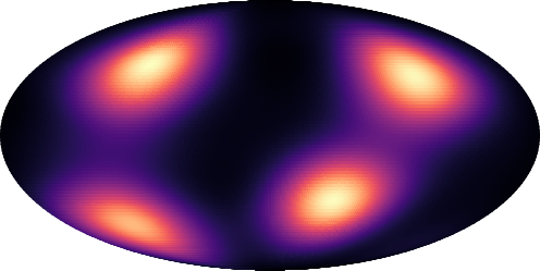
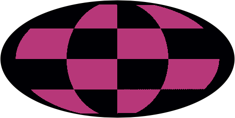
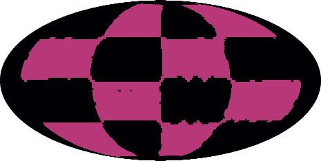
Figure 3: Learned RCPMs on the sphere. Following Rezende et al. (2020), we learn the first density with the reverse KL, and following Lou et al. (2020), we learn the second with maximum likelihood.

Results are logged in table 1. Notably, our model significantly outperforms both baseline models with a KL of $0.003$, almost an order of magnitude smaller than the runner-up with a KL of $0.05$. This highlights the expressive power of the RCPM model class. We also provide a visualization of the trained RCPM in fig. 3 (top row), where we show KDE estimates performed in spherical coordinates with a bandwidth of 0.2. Finally, table 2 compares the runtime per training iteration of our model with Rezende et al. (2020)’s models over 1000 trials with a batch size of 256. Our model’s speed is comparable to theirs while leading to significantly improved KL/ESS.

Likelihood training.

We demonstrate an RCPM trained via maximum likelihood on a more challenging dataset, the checkerboard, also studied in Lou et al. (2020). Figure 3 (bottom) shows the RCPM generated density on the right. We found visualizing the density of our model challenging because some regions had unusually high density values around the poles. We hence binarized the density plot. We provide the original density in fig. 9 (Supplementary).

6.2 Torus

Base	RCPM	Target

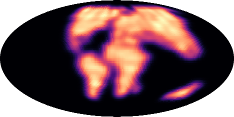
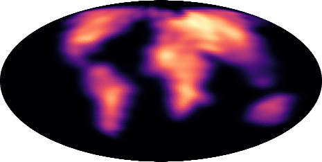
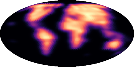
Figure 4: We trained a 7-block RCPM flow to learn to map a base density over ground mass on earth of $90$ million years ago such a density over current earth. To learn, we minimize the KL divergence between the model and the target distribution.

True	RCPM

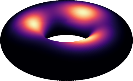
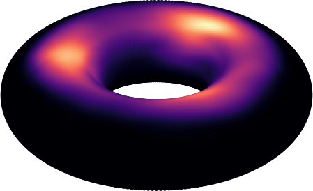
Figure 5: We trained an RCPM $\nu_{\theta}$ to learn a $3$-modal density $\nu$ on the torus $T^{2}={\mathcal{S}}^{1}\times{\mathcal{S}}^{1}$ (KL: $0.03$, ESS: $94.7$).

We now consider an experiment on the torus: ${\mathcal{T}}^{2}={\mathcal{S}}^{1}\times{\mathcal{S}}^{1}$. The exponential map and intrinsic distance required for RCPMs are known in closed-form. The exponential map flows in Rezende et al. (2020) do not apply to this setting as their $c$-concave layers are specific to the sphere.

We train a 6-block RCPM model (with 1 layer per block) by KL minimization. As can be inspected from fig. 5, the RCPM model is able to recover the target density accurately, and the model achieves a KL of $0.03$ and an ESS of $94.7$.

6.3 Case Study: Continental Drift

Finally, we consider a real-world application of our model on geological data in the context of continental drift (Wilson, 1963). We aim to demonstrate the versatility and flexibility of the framework with three distinct settings: mapping estimation, density estimation, and geodesic transport, all through the lens of RCPMs.

Mapping estimation.

We begin with mapping estimation. We aim to learn a flow $t$ mapping the base distribution of ground mass on earth $90$ million years ago (fig. 4, left), to a ground mass distribution on current earth (fig. 4, right) – the target. We train a $7$-blocks RCPM with $3$-layers blocks (see sect. 5.1) by minimizing the KL divergence between the model and target distributions. In fig. 4 (Middle), we show the RCPM result, where it successfully learns to recover the target density over current earth. Hence, the mapping $t$ can be used to map mass from “old” earth to current earth.

Transport geodesics.

We demonstrate the use of transport geodesics induced by exponential-map flows. We train a $1$-block RCPM which allows to recover approximations of optimal-transport geodesics following eq. 10. These curves are induced by transport mappings $\exp(t\nabla\phi),t\in[0,1]$, which we visualize for a grid of starting points $x_{0}$ on the sphere in fig. 6. Such geodesics illustrate the optimal transport evolution of earth ground across times. This relates to the well-known and studied geological process of continental drift (Wilson, 1963). North-American and Eurasian tectonic plates move away from each other at a small rate per year, which is illustrated in eq. 10. Denote as “junction” the junction between Eurasian and North-American continents in “old” earth. We observe that particles $x_{0}$ located at the right of the junction will have geodesics transporting them towards the right, while particles located at the left of such junction will be transported towards the left, which is the expected behavior given the evolution of continental locations across time (see fig. 4 left and right).

Density estimation.

Finally, we consider RCPMs as density estimation tools. In this setting, we aim to learn a flow from a known base distribution (e.g., uniform on the sphere) to a target distribution (e.g., distribution of mass over earth) given samples from the latter. We train an RCPM model with $6$ blocks (and $1$ layer per block) by maximum likelihood. We show the results for this experiment in fig. 7. We observe that the model is able to recover the distribution of mass on current earth.

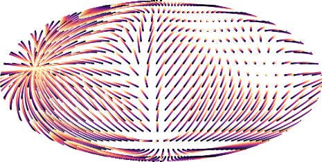
Figure 6: Plot of the transport geodesics arising from a 1-block RCPM trained in the setting of fig. 4, and following eq. 10. We observe that samples stretch according to continental movements.

True	RCPM

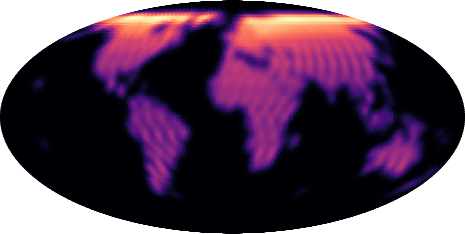
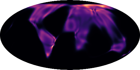
Figure 7: We trained a 6-block RCPM in the density estimation setting. The base distribution is the uniform distribution on the sphere and the target $\nu$ is the ground of current earth.

7 Conclusion

In this paper, we propose to build flows on compact Riemannian manifolds following the celebrated theory of McCann (2001), that is using exponential map applied to gradients of $c$-concave functions. Our main contribution is observing that the rather intricate space of $c$-concave functions over arbitrary compact Riemannian manifold can be approximated with discrete $c$-concave functions. We provide a theoretical result showing that discrete $c$-concave functions are dense in the space of $c$-concave functions. We use this theoretical result to prove that maps defined via a discrete $c$-concave potentials are universal. Namely, can approximate arbitrary optimal transports between an absolutely continuous source distribution and arbitrary target distribution on the manifold.

We build upon this theory to design a practical model, RCPM, that can be applied to any manifold where the exponential map and the intrinsic distance are known, and enjoys maximal expressive power. We experimented with RCPM, and used it to train flows on spheres and tori, on both synthetic and real data. We observed that RCPM outperforms previous approaches on standard manifold flow tasks. We also provided a case study demonstrating the potential of RCPMs for applications in geology.

Future work includes training flows on more general manifolds, e.g., manifolds defined with signed distance functions, and using RCPM on other manifold learning tasks where the expressive power of RCPM can potentially make a difference. One particular interesting venue is generalizing the estimation of barycenters (means) of probability measures on Euclidean spaces to the Riemannian setting through the use of discrete $c$-concave functions.

Appendix A Manifold Operations

We briefly describe manifold operations, on a Riemannian manifold ${\mathcal{M}}$ with metric $g$, used in this paper. Specifically, we define the exponential map $\exp$ and the intrinsic manifold distance $d_{{\mathcal{M}}}$.

Exponential map.

Let $x\in{\mathcal{M}}$, $v\in T_{x}{\mathcal{M}}$ and consider the unique geodesic $\gamma:[0,1]\rightarrow{\mathcal{M}}$ such that $\gamma(0)=x$ and $\gamma^{\prime}(0)=v$. The exponential map at $x$, $\exp_{x}:T_{x}{\mathcal{M}}\rightarrow{\mathcal{M}}$, is defined as

$$\exp_{x}(v)=\gamma(1).$$ (26)

Intrinsic distance.

Define the length of a curve $\gamma:[0,1]\rightarrow{\mathcal{M}}$ as

$$L(\gamma)=\int_{0}^{1}\left\|\gamma^{\prime}(t)\right\|_{g}dt,$$ (27)

where $\left\|\gamma^{\prime}(t)\right\|_{g}$ means taking the norm of the velocity $\gamma^{\prime}(t)$ at $T_{\gamma(t)}{\mathcal{M}}$ with respect to the metric $g$ of the manifold ${\mathcal{M}}$. Then, the intrinsic distance $d_{{\mathcal{M}}}$ between $x,y\in{\mathcal{M}}$ is:

$$d_{{\mathcal{M}}}(x,y)=\inf_{\gamma}L(\gamma)$$ (28)

where the $\inf$ is over curves $\gamma:[0,1]\rightarrow{\mathcal{M}}$ where $\gamma(0)=x$ and $\gamma(1)=y$. If ${\mathcal{M}}$ is complete (see e.g., Hopf-Rinow Theorem) the intrinsic distance is realized by a geodesic.

Sphere.

On the $n$-sphere ${\mathcal{S}}^{n}$, the exponential map and the intrinsic distance are provided as closed-form expressions. If $x,y\in{\mathcal{S}}^{n}$ and $v\in T_{x}{\mathcal{S}}^{n}$,

$$\exp_{x}(v)=x\cos(\left\|v\right\|)+\frac{v}{\left\|v\right\|}\sin(\left\|v\right\|)$$ (29)

$$d_{{\mathcal{S}}^{n}}(x,y)=\arccos(x^{T}y),$$ (30)

where $\left\|\cdot\right\|$ is the standard Euclidean norm.

Product manifolds.

We now consider operations on product manifolds of the form ${\mathcal{M}}={\mathcal{M}}_{1}\times\ldots\times{\mathcal{M}}_{l}$. The squared intrinsic distance is simply

$$d^{2}_{{\mathcal{M}}}(x,y)=d^{2}_{{\mathcal{M}}_{1}}(x_{1},y_{1})+\ldots+d^{2}_{{\mathcal{M}}_{l}}(x_{l},y_{l}).$$ (31)

Here $x=(x_{1},\ldots,x_{l})$, and $x_{j}\in{\mathcal{M}}_{j},\ \ j\in[l]$ (and similarly for $y$). The exponential map on the product manifold is the cartesian product of exponential maps on the individual manifolds. An instantiation of such product that will be considered in experiments is the torus ${\mathcal{S}}^{1}\times{\mathcal{S}}^{1}$. In that case, we can use eqs. 29 and 30 to get the exponential map and squared intrinsic distance in closed-form.

Appendix B Proof of c-concavity of the multi-layer potential

Proof.

The proof is by induction. Constant functions are c-concave, hence $\psi_{0}$ is c-concave. Also, $\psi_{1}=(1-w_{0})\phi_{0}$ is c-concave by the assumption of convexity of the space of $c$-concave functions. Next, assuming $\psi_{k-1}(x)$ is c-concave, $\sigma(\psi_{k-1})$ is also c-concave (because $\sigma$ preserves $c$-concavity), and $\psi_{k}(x)$ is c-concave because convex combinations of $c$-concave functions are $c$-concave. In conclusion, $\varphi=\psi_{K}$ is $c$-concave ∎

Appendix C Additional experimental and implementation details

C.1 Synthetic Sphere

We conducted a hyper-parameter search over the parameters in table 3 to find the flows used in our demonstrations and experiments. We report results from the best hyper-parameters obtained by randomly sampling the space of parameters. The $\alpha$ values are initialized from ${\mathcal{U}}[\alpha_{\rm min},\alpha_{\rm min}+\alpha_{\rm range}]$. Also, $\gamma_{1}$ corresponds to the softing coefficient of the soft-min operation of discrete $c$-concave potentials, and $\gamma_{2}$ to the softing coefficient of the soft-min operation in the identity initialization (see sects. 5.1 and 5.3).

Table 3: Hyper-parameter sweep for our sphere results

Adam
learning rate	[$10^{-6}$, $10^{-1}$]
$\beta_{1}$	[0.1, 0.3, 0.5, 0.7, 0.9]
$\beta_{2}$	[0.1, 0.3, 0.5, 0.7, 0.9, 0.99, 0.999]
Flow Hyper-parameters
Nb. of Components $y_{i}$	[50, 1000]
$\alpha_{\rm min}$	[$10^{-5}$, 10]
$\alpha_{\rm range}$	[$10^{-3}$, 1]
$\gamma_{1}$	[0.01, 0.05, 0.1, 0.5]
$\gamma_{2}$	[None, 0.01, 0.05, 0.1, 0.5]

We now verify empirically whether the RPCM define diffeomorphisms in practice. We compute Jacobian log-determinants of the flow trained on the $4$-modal density taken from Rezende et al. (2020) for $10^{6}$ points uniformly sampled on the sphere, and observe that all these are positive (see fig. 8).

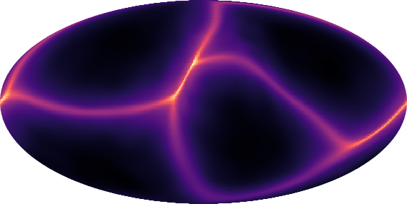
Figure 8: Jacobian log-determinants for points uniformly sampled on the sphere.

Binarized checkerboard density.

We found it difficult to visualize the learned density of our model on the checkerboard because a few regions have unusually high values that mess up the ranges of the colormap. For visualization purposes, we binarize the density values by taking the portion of the density greater than the uniform density. Figure 9 shows the original and binarized densities of our models.

Original Density	Binarized Density

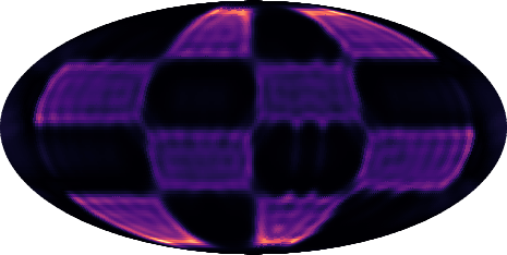
Figure 9: Binarized density of the sphere checkerboard

C.2 Torus

Model.

We provide details on the model used in the torus demonstration. The RCPM is composed of $6$ single-layer blocks of $200$ components, and the softing parameter is set to $0.5$. Adam’s learning rate is set to $6e^{-4}$ and $\beta$ to $(0.9,0.99)$.

Data.

The target density is of a form inspired by the target densities in Rezende et al. (2020)):

$$p(\theta_{1},\theta_{2}) =\frac{1}{3}\sum_{i=1}^{3}p_{i}(\theta_{1},\theta_{2})$$ (32)

$$p_{i}(\theta_{1},\theta_{2}) \propto\exp{[\cos(\theta_{1}-a^{1}_{i})+\cos(\theta_{2}-a^{2}_{i})]}$$ (33)

where $a_{1}=[4.18,6.7],a_{2}=[4.18,4.7],a_{3}=[4.18,2.7]$, and $\theta_{1},\theta_{2}\in[0,2\pi]$.

C.3 Continental Drift

Mapping estimation.

We continue with details on the model used in the mapping estimation setting of the continental drift case study. The RCPM is composed of $7$ blocks containing each $3$ layers with $200$ components, and the softing coefficient is set to $0.2$. Adam’s learning rate is set to $2e^{-3}$ and $\beta=(0.9,0.99)$.

Transport geodesics.

We now discuss the transport geodesics setting. The RCPM is composed of a single block (hence allowing to recover the optimal transport geodesics) containing $3$ layers with $200$ components, and the softing coefficient is set to $\gamma=0.2$. Adam’s learning rate is set to $2e^{-3}$ and $\beta=(0.9,0.99)$.

Density estimation.

Finally, we provide details on the model used in the density estimation setting. The RCPM is composed of $6$ single-layer blocks containing each $400$ components, and the softing coefficient is set to $6e^{-2}$. Adam’s learning rate is set to $2e^{-3}$ and $\beta=(0.9,0.99)$.

Data.

The earth densities are obtained by leveraging the code from https://github.com/cgarciae/point-cloud-mnist-2D to turn Mollweide earth images into spherical point clouds, converting to Euclidean coordinates, and applying kernel density estimation to such point clouds both for visualization, and to get log-probabilities when they are required (e.g., in the mapping estimation setting, where access to log-probabilities from the base – old earth – is needed to train the model).

References

- Alvarez-Melis et al. (2020) Alvarez-Melis, D., Mroueh, Y., and Jaakkola, T. Unsupervised hierarchy matching with optimal transport over hyperbolic spaces. In Proceedings of the Twenty Third International Conference on Artificial Intelligence and Statistics, pp. 1606–1617, 2020.
- Amos et al. (2017) Amos, B., Xu, L., and Kolter, J. Z. Input convex neural networks. In International Conference on Machine Learning, pp. 146–155, 2017.
- Bose et al. (2020) Bose, J., Smofsky, A., Liao, R., Panangaden, P., and Hamilton, W. Latent variable modelling with hyperbolic normalizing flows. In International Conference on Machine Learning, pp. 1045–1055. PMLR, 2020.
- Bradbury et al. (2018) Bradbury, J., Frostig, R., Hawkins, P., Johnson, M. J., Leary, C., Maclaurin, D., Necula, G., Paszke, A., VanderPlas, J., Wanderman-Milne, S., and Zhang, Q. JAX: composable transformations of Python+NumPy programs, 2018. URL http://github.com/google/jax.
- Brehmer & Cranmer (2020) Brehmer, J. and Cranmer, K. Flows for simultaneous manifold learning and density estimation. arXiv preprint arXiv:2003.13913, 2020.
- Chen et al. (2018) Chen, R. T. Q., Rubanova, Y., Bettencourt, J., and Duvenaud, D. Neural ordinary differential equations. In Proceedings of the 32nd International Conference on Neural Information Processing Systems, pp. 6572–6583, 2018.
- Cuturi & Blondel (2017) Cuturi, M. and Blondel, M. Soft-dtw: A differentiable loss function for time-series. In Proceedings of the 34th International Conference on Machine Learning - Volume 70, pp. 894–903, 2017.
- Dinh et al. (2016) Dinh, L., Sohl-Dickstein, J., and Bengio, S. Density estimation using real nvp. arXiv preprint arXiv:1605.08803, 2016.
- Figalli & Rifford (2009) Figalli, A. and Rifford, L. Continuity of optimal transport maps and convexity of injectivity domains on small deformations of s2. Communications on Pure and Applied Mathematics: A Journal Issued by the Courant Institute of Mathematical Sciences, 62(12):1670–1706, 2009.
- Figalli & Villani (2011) Figalli, A. and Villani, C. Optimal Transport and Curvature, pp. 171–217. Springer Berlin Heidelberg, Berlin, Heidelberg, 2011. ISBN 978-3-642-21861-3. doi: 10.1007/978-3-642-21861-3˙4. URL https://doi.org/10.1007/978-3-642-21861-3_4.
- Figalli et al. (2010a) Figalli, A., Kim, Y.-H., and McCann, R. Regularity of optimal transport maps on multiple products of spheres. Journal of the European Mathematical Society, 15, 06 2010a. doi: 10.4171/JEMS/388.
- Figalli et al. (2010b) Figalli, A., Kim, Y.-H., and McCann, R. Regularity of optimal transport maps on multiple products of spheres. Journal of the European Mathematical Society, 15, 06 2010b. doi: 10.4171/JEMS/388.
- Gangbo & McCann (1996) Gangbo, W. and McCann, R. J. The geometry of optimal transportation. Acta Math., 177(2):113–161, 1996. doi: 10.1007/BF02392620. URL https://doi.org/10.1007/BF02392620.
- Goodfellow et al. (2014) Goodfellow, I. J., Pouget-Abadie, J., Mirza, M., Xu, B., Warde-Farley, D., Ozair, S., Courville, A., and Bengio, Y. Generative adversarial nets. In Proceedings of the 27th International Conference on Neural Information Processing Systems - Volume 2, pp. 2672–2680, 2014.
- Haarnoja et al. (2018) Haarnoja, T., Hartikainen, K., Abbeel, P., and Levine, S. Latent space policies for hierarchical reinforcement learning. In Proceedings of the 35th International Conference on Machine Learning, pp. 1851–1860, 2018.
- Hoyos-Idrobo (2020) Hoyos-Idrobo, A. Aligning hyperbolic representations: an optimal transport-based approach. arXiv: Machine Learning, 2020.
- Huang et al. (2020) Huang, C.-W., Chen, R. T. Q., Tsirigotis, C., and Courville, A. Convex potential flows: Universal probability distributions with optimal transport and convex optimization, 2020.
- Hunter (2007) Hunter, J. D. Matplotlib: A 2d graphics environment. Computing in science & engineering, 9(3):90, 2007.
- Jones et al. (2014) Jones, E., Oliphant, T., and Peterson, P. SciPy: Open source scientific tools for Python. 2014.
- Kim & McCann (2012) Kim, Y.-H. and McCann, R. J. Towards the smoothness of optimal maps on riemannian submersions and riemannian products (of round spheres in particular). Journal für die reine und angewandte Mathematik, 2012(664):1–27, 2012.
- Kingma & Welling (2014) Kingma, D. P. and Welling, M. Auto-encoding variational bayes. In 2nd International Conference on Learning Representations, 2014.
- Kluyver et al. (2016) Kluyver, T., Ragan-Kelley, B., Pérez, F., Granger, B. E., Bussonnier, M., Frederic, J., Kelley, K., Hamrick, J. B., Grout, J., Corlay, S., et al. Jupyter notebooks-a publishing format for reproducible computational workflows. In ELPUB, pp. 87–90, 2016.
- Köhler et al. (2019) Köhler, J., Klein, L., and Noé, F. Equivariant flows: sampling configurations for multi-body systems with symmetric energies. ArXiv, abs/1910.00753, 2019.
- Kong & Chaudhuri (2020) Kong, Z. and Chaudhuri, K. The expressive power of a class of normalizing flow models. In Proceedings of the Twenty Third International Conference on Artificial Intelligence and Statistics, pp. 3599–3609, 2020.
- Korotin et al. (2021) Korotin, A., Egiazarian, V., Asadulaev, A., Safin, A., and Burnaev, E. Wasserstein-2 generative networks. In International Conference on Learning Representations, 2021. URL https://openreview.net/forum?id=bEoxzW_EXsa.
- Lee & Li (2012) Lee, P. W. Y. and Li, J. New examples satisfying ma-trudinger-wang conditions. SIAM J. Math. Anal., 44(1):61–73, 2012. doi: 10.1137/110820543. URL https://doi.org/10.1137/110820543.
- Loeper (2009) Loeper, G. On the regularity of solutions of optimal transportation problems. Acta Math., 202(2):241–283, 2009. doi: 10.1007/s11511-009-0037-8. URL https://doi.org/10.1007/s11511-009-0037-8.
- Lou et al. (2020) Lou, A., Lim, D., Katsman, I., Huang, L., Jiang, Q., Lim, S. N., and De Sa, C. M. Neural manifold ordinary differential equations. Advances in Neural Information Processing Systems, 33, 2020.
- Lucet (1997) Lucet, Y. Faster than the fast legendre transform, the linear-time legendre transform. Numerical Algorithms, 16(2):171–185, 1997.
- Makkuva et al. (2020) Makkuva, A., Taghvaei, A., Oh, S., and Lee, J. Optimal transport mapping via input convex neural networks. In Proceedings of the 37th International Conference on Machine Learning, pp. 6672–6681, 2020.
- Makkuva et al. (2019) Makkuva, A. V., Taghvaei, A., Oh, S., and Lee, J. D. Optimal transport mapping via input convex neural networks. arXiv preprint arXiv:1908.10962, 2019.
- Mathieu & Nickel (2020) Mathieu, E. and Nickel, M. Riemannian continuous normalizing flows. Advances in Neural Information Processing Systems, 33, 2020.
- McCann (2001) McCann, R. J. Polar factorization of maps on riemannian manifolds. Geometric & Functional Analysis GAFA, 11(3):589–608, 2001.
- McKinney (2012) McKinney, W. Python for data analysis: Data wrangling with Pandas, NumPy, and IPython. ” O’Reilly Media, Inc.”, 2012.
- Oliphant (2006) Oliphant, T. E. A guide to NumPy, volume 1. Trelgol Publishing USA, 2006.
- Oliphant (2007) Oliphant, T. E. Python for scientific computing. Computing in Science & Engineering, 9(3):10–20, 2007.
- Papamakarios et al. (2019) Papamakarios, G., Nalisnick, E. T., Rezende, D. J., Mohamed, S., and Lakshminarayanan, B. Normalizing flows for probabilistic modeling and inference. abs/1912.02762, 2019.
- Peyre & Cuturi (2019) Peyre, G. and Cuturi, M. Computational optimal transport: With applications to data science. Foundations and Trends in Machine Learning, 11(5-6):355–607, 2019.
- Rezende & Mohamed (2015) Rezende, D. and Mohamed, S. Variational inference with normalizing flows. In Proceedings of the 32nd International Conference on Machine Learning, pp. 1530–1538, 2015.
- Rezende et al. (2014) Rezende, D. J., Mohamed, S., and Wierstra, D. Stochastic backpropagation and approximate inference in deep generative models. In Proceedings of the 31st International Conference on Machine Learning, pp. 1278–1286, 2014.
- Rezende et al. (2019) Rezende, D. J., Racanière, S., Higgins, I., and Toth, P. Equivariant hamiltonian flows. In ML for Physical Sciences, NeurIPS 2019 Worshop, 2019.
- Rezende et al. (2020) Rezende, D. J., Papamakarios, G., Racanière, S., Albergo, M. S., Kanwar, G., Shanahan, P. E., and Cranmer, K. Normalizing flows on tori and spheres. arXiv preprint arXiv:2002.02428, 2020.
- Sei (2013) Sei, T. A jacobian inequality for gradient maps on the sphere and its application to directional statistics. Communications in Statistics-Theory and Methods, 42(14):2525–2542, 2013.
- Takashi (1996) Takashi, S. Riemannian geometry / Takashi Sakai ; translated by Takashi Sakai. Translations of mathematical monographs. American Mathematical Society, Providence, R.I, 1996. ISBN 0-8218-0284-4.
- Van Der Walt et al. (2011) Van Der Walt, S., Colbert, S. C., and Varoquaux, G. The numpy array: a structure for efficient numerical computation. Computing in Science & Engineering, 13(2):22, 2011.
- Van Rossum & Drake Jr (1995) Van Rossum, G. and Drake Jr, F. L. Python reference manual. Centrum voor Wiskunde en Informatica Amsterdam, 1995.
- Villani (2008) Villani, C. Optimal transport: old and new, volume 338. Springer Science & Business Media, 2008.
- Wilson (1963) Wilson, J. T. Continental drift. Scientific American, 208(4):86–103, 1963. ISSN 00368733, 19467087. URL http://www.jstor.org/stable/24936535.
- Yadan (2019) Yadan, O. Hydra - a framework for elegantly configuring complex applications. Github, 2019. URL https://github.com/facebookresearch/hydra.