MADE: Exploration via Maximizing Deviation from Explored Regions

Abstract

In online reinforcement learning (RL), efficient exploration remains particularly challenging in high-dimensional environments with sparse rewards. In low-dimensional environments, where tabular parameterization is possible, count-based upper confidence bound (UCB) exploration methods achieve minimax near-optimal rates. However, it remains unclear how to efficiently implement UCB in realistic RL tasks that involve non-linear function approximation. To address this, we propose a new exploration approach via maximizing the deviation of the occupancy of the next policy from the explored regions. We add this term as an adaptive regularizer to the standard RL objective to balance exploration vs. exploitation. We pair the new objective with a provably convergent algorithm, giving rise to a new intrinsic reward that adjusts existing bonuses. The proposed intrinsic reward is easy to implement and combine with other existing RL algorithms to conduct exploration. As a proof of concept, we evaluate the new intrinsic reward on tabular examples across a variety of model-based and model-free algorithms, showing improvements over count-only exploration strategies. When tested on navigation and locomotion tasks from MiniGrid and DeepMind Control Suite benchmarks, our approach significantly improves sample efficiency over state-of-the-art methods. Our code is available at https://github.com/tianjunz/MADE.

1 Introduction

Online RL is a useful tool for an agent to learn how to perform tasks, particularly when expert demonstrations are unavailable and reward information needs to be used instead Sutton and Barto (2018). To learn a satisfactory policy, an RL agent needs to effectively balance between exploration and exploitation, which remains a central question in RL (Ecoffet et al., 2019; Burda et al., 2018b). Exploration is particularly challenging in environments with sparse rewards. One popular approach to exploration is based on intrinsic motivation, often applied by adding an intrinsic reward (or bonus) to the extrinsic reward provided by the environment. In provable exploration methods, bonus often captures the value estimate uncertainty and the agent takes an action that maximizes the upper confidence bound (UCB) Agrawal and Jia (2017); Azar et al. (2017); Jaksch et al. (2010); Kakade et al. (2018); Jin et al. (2018). In tabular setting, UCB bonuses are often constructed based on either Hoeffding’s inequality, which only uses visitation counts, or Bernstein’s inequality, which uses value function variance in addition to visitation counts. The latter is proved to be minimax near-optimal in environments with bounded rewards Jin et al. (2018); Menard et al. (2021) as well as bounded total reward Zhang et al. (2020b) and reward-free settings Ménard et al. (2020); Kaufmann et al. (2021); Jin et al. (2020a); Zhang et al. (2020c). It remains an open question how one can efficiently compute confidence bounds to construct UCB bonus in non-linear function approximation. Furthermore, Bernstein-style bonuses are often hard to compute in practice beyond tabular setting, due to difficulties in computing value function variance.

In practice, various approaches are proposed to design intrinsic rewards: visitation pseudo-count bonuses estimate count-based UCB bonuses using function approximation (Bellemare et al., 2016; Burda et al., 2018b), curiosity-based bonuses seek states where model prediction error is high, uncertainty-based bonuses (Pathak et al., 2019; Shyam et al., 2019) adopt ensembles of networks for estimating variance of the Q-function, empowerment-based approaches (Klyubin et al., 2005; Gregor et al., 2016; Salge et al., 2014; Mohamed and Rezende, 2015) lead the agent to states over which the agent has control, and information gain bonuses (Kim et al., 2018) reward the agent based on the information gain between state-action pairs and next states.

Although the performance of practical intrinsic rewards is good in certain domains, empirically they are observed to suffer from issues such as detachment, derailment, and catastrophic forgetting Agarwal et al. (2020a); Ecoffet et al. (2019). Moreover, these methods usually lack a clear objective and can get stuck in local optimum Agarwal et al. (2020a). Indeed, the impressive performance currently achieved by some deep RL algorithms often revolves around manually designing dense rewards Brockman et al. (2016), complicated exploration strategies utilizing a significant amount of domain knowledge Ecoffet et al. (2019), or operating in the known environment regime Silver et al. (2017); Moravčík et al. (2017).

Motivated by current practical challenges and the gap between theory and practice, we propose a new algorithm for exploration by maximizing deviation from explored regions. This yields a practical algorithm with strong empirical performance. To be specific, we make the following contributions:

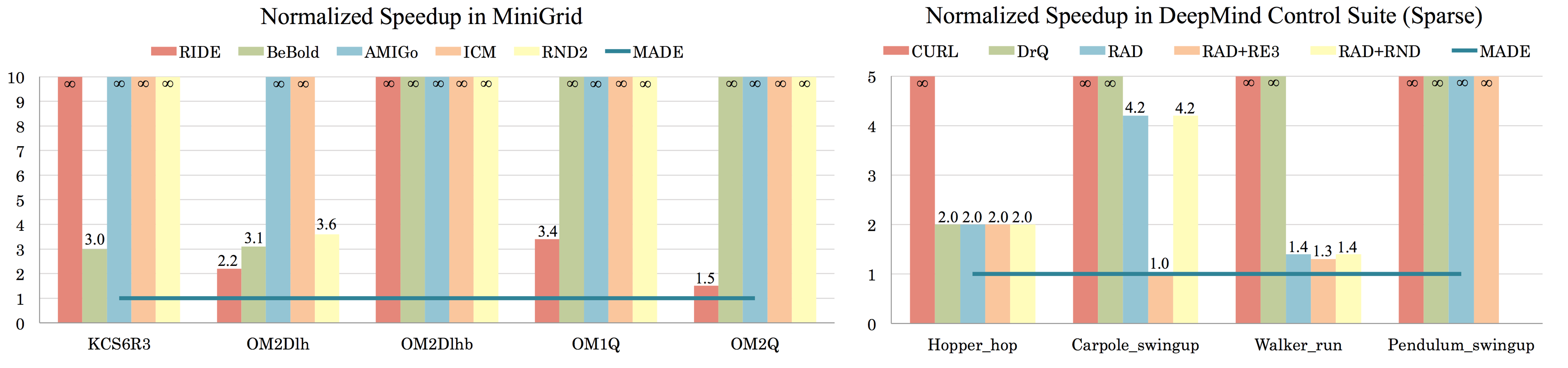
Figure 1: Normalized samples use of different methods with respect to MADE (smaller values are better). MADE consistency achieves a better sample efficiency compared to all other baselines. Infinity means the method fails to achieve maximum reward in given steps.

1. Exploration via maximizing deviation

Our approach is based on modifying the standard RL objective (i.e. the cumulative reward) by adding a regularizer that adaptively changes across iterations. The regularizer can be a general function depending on the state-action visitation density and previous state-action coverage. We then choose a particular regularizer that MAximizes the DEviation (MADE) of the next policy visitation $d^{\pi}$ from the regions covered by prior policies $\rho^{k}_{\text{cov}}$:

$$L_{k}(d^{\pi})={J(d^{\pi})}+{\tau_{k}\sum_{s,a}\sqrt{\tfrac{d^{\pi}(s,a)}{\rho^{k}_{\text{cov}}(s,a)}}}.$$ (1)

Here, $k$ is the iteration number, $J(d^{\pi})$ is the standard RL objective, and the regularizer encourages $d^{\pi}(s,a)$ to be large when $\rho^{k}_{\text{cov}}(s,a)$ is small. We give an algorithm for solving the regularized objective and prove that with access to an approximate planning oracle, it converges to the global optimum. We show that objective (1) results in an intrinsic reward that can be easily added to any RL algorithm to improve performance, as suggested by our empirical studies. Furthermore, the intrinsic reward applies a simple modification to the UCB-style bonus that considers prior visitation counts. This simple modification can also be added to existing bonuses in practice.

2. Tabular studies

In the special case of tabular parameterization, we show that MADE only applies some simple adjustments to the Hoeffding-style count-based bonus. We compare the performance of MADE to Hoeffding and Bernstein bonuses in three different RL algorithms, for the exploration task in the stochastic diabolical bidirectional lock Agarwal et al. (2020a); Misra et al. (2020), which has sparse rewards and local optima. Our results show that MADE robustly improves over the Hoeffding bonus and is competitive to the Bernstein bonus, across all three RL algorithms. Interestingly, MADE bonus and exploration strategy appear to be very close to the Bernstein bonus, without computing or estimating variance, suggesting that MADE potentially captures some environmental structures. Additionally, we empirically show that MADE regularizer can improve the optimization rate in policy gradient methods.

3. Experiments on MiniGrid and DeepMind Control Suite

We empirically show that MADE works well when combined with model-free (IMAPLA (Espeholt et al., 2018), RAD (Laskin et al., 2020)) and model-based (Dreamer (Hafner et al., 2019)) RL algorithms, greatly improving the sample efficiency over existing baselines. When tested in the procedurally-generated MiniGrid environments, MADE manages to converge with two to five times fewer samples compared to state-of-the-art method BeBold (Zhang et al., 2020a). In DeepMind Control Suite (Tassa et al., 2020), we build upon the model-free method RAD (Laskin et al., 2020) and the model-based method Dreamer (Hafner et al., 2019), improving the return up to 150 in 500K steps compared to baselines. Figure 1 shows normalized sample size to achieve maximum reward with respect to our algorithm.

2 Background

Markov decision processes.

An infinite-horizon discounted MDP is described by a tuple $M=(\mathcal{S},\mathcal{A},P,r,\rho,\gamma)$, where $\mathcal{S}$ is the state space, $\mathcal{A}$ is the action space, $P:\mathcal{S}\times\mathcal{A}\mapsto\Delta(\mathcal{S})$ is the transition kernel, $r:\mathcal{S}\times\mathcal{A}\mapsto[0,1]$ is the (extrinsic) reward function, $\rho:\mathcal{S}\mapsto\Delta(\mathcal{S})$ is the initial distribution, and $\gamma\in[0,1)$ is the discount factor. A stationary (stochastic) policy $\pi\in\Delta(\mathcal{A}\mid\mathcal{S})$ specifies a distribution over actions in each state. Each policy $\pi$ induces a visitation density over state-action pairs $d^{\pi}:\mathcal{S}\times\mathcal{A}\mapsto[0,1]$ defined as $d^{\pi}_{\rho}(s,a)\coloneqq(1-\gamma)\sum_{t=0}^{\infty}\gamma^{t}\operatorname{\mathbb{P}}_{t}(s_{t}=s,a_{t}=a;\pi)$, where $\operatorname{\mathbb{P}}_{t}(s_{t}=s,a_{t}=a;\pi)$ denotes $(s,a)$ visitation probability at step $t$, starting at $s_{0}\sim\rho(\cdot)$ and following $\pi$. An important quantity is the value a policy $\pi$, which is the discounted sum of rewards $V^{\pi}(s)\coloneqq\operatorname{\mathbb{E}}[\sum_{t=0}^{\infty}\gamma^{t}r_{t}\;|\;s_{0}=s,a_{t}\sim\pi(\cdot\mid s_{t})\text{ for all }t\geq 0]$ starting at state $s\in\mathcal{S}$.

Policy mixture.

For a sequence of policies $\mathcal{C}^{k}=(\pi_{1},\dots,\pi_{k})$ with corresponding mixture distribution $w^{k}\in\Delta_{k-1}$, the policy mixture $\pi_{\operatorname*{mix},k}=(\mathcal{C}^{k},w^{k})$ is obtained by first sampling a policy from $w^{k}$ and then following that policy over subsequent steps Hazan et al. (2019). The mixture policy induces a state-action visitation density according to $d^{\pi_{\operatorname*{mix}}}(s,a)=\sum_{i=1}^{k}w_{i}^{k}d^{\pi_{i}}(s,a).$ While the $\pi_{\operatorname*{mix}}$ may not be stationary in general, there exists a stationary policy $\pi^{\prime}$ such that $d^{\pi^{\prime}}=d^{\pi_{\operatorname*{mix}}}$; see Puterman (1990) for details.

Online reinforcement learning.

Online RL is the problem of finding a policy with a maximum value from an unknown MDP, using samples collected during exploration. Oftentimes, the following objective is considered, which is a scalar summary of the performance of policy $\pi$:

$$J_{M}(\pi)\coloneqq\operatorname{\mathbb{E}}_{s\sim\rho}[V^{\pi}(s)]=({1-\gamma})^{-1}\operatorname{\mathbb{E}}_{(s,a)\sim d^{\pi}_{\rho}(\cdot,\cdot)}[r(s,a)].$$ (2)

We drop index $M$ when it is clear from context. We denote an optimal policy by $\pi^{\star}\in\operatorname*{arg\,max}_{\pi}J(\pi)$ and use the shorthand $V^{\star}\coloneqq V^{\pi^{\star}}$ to denote the optimal value function. It is straightforward to check that $J(\pi)$ can equivalently be represented by the expectation of the reward over the visitation measure of $\pi$. We slightly abuse the notation and sometimes write $J(d^{\pi})$ to denote the RL objective.

3 Adaptive regularization of the RL objective

3.1 Regularization to guide exploration

In online RL, the agent faces a dilemma in each state: whether it should select a seemingly optimal policy (exploit) or it should explore different regions of the MDP. To allow flexibility in this choice and trade-off between exploration and exploitation, we propose to add a regularizer to the standard RL objective that changes throughout iterations of an online RL algorithm:

$$L_{k}(d^{\pi})=\underbrace{J(d^{\pi})}_{\text{exploitation}}+\tau_{k}\underbrace{R(d^{\pi};\{d^{\pi_{i}}\}_{i=1}^{k})}_{\text{exploration}}.$$ (3)

Here, $R(d^{\pi};\{d^{\pi_{i}}\}_{i=1}^{k})$ is a function of state-action visitation of $\pi$ as well as the visitation of prior policies $\pi_{1},\dots,\pi_{k}$. The temperature parameter $\tau_{k}$ determines the strength of regularization. Objective (3) is a population objective in the sense that it does not involve empirical estimations affected by the randomness in sample collection. In the following section, we give our particular choice of regularizer and discuss how this objective can describe some popular exploration bonuses. We then provide a convergence guarantee for the regularized objective in Section 3.2.

3.2 Exploration via maximizing deviation from policy cover

We develop our exploration strategy MADE based on a simple intuition: maximizing the deviation from the explored regions, i.e. all states and actions visited by prior policies. We define policy cover at iteration $k$ to be the density over regions explored by policies $\pi_{1},\dots,\pi_{k}$, i.e. $\rho_{\text{cov}}^{k}(s,a)\coloneqq\frac{1}{k}\sum_{i=1}^{k}d^{\pi_{i}}(s,a).$ We then design our regularizer to encourage $d^{\pi}$ to be different from $\rho_{\text{cov}}^{k}$:

$$R_{k}(d^{\pi};\{d^{\pi_{i}}\}_{i=1}^{k})=\sum_{s,a}\sqrt{\frac{d^{\pi}(s,a)}{\rho_{\text{cov}}^{k}(s,a)}}.$$ (4)

It is easy to check that the maximizer of above function is $d^{\pi}(s,a)\propto\frac{1}{\rho_{\text{cov}}^{k}(s,a)}$. Our motivation behind this particular deviation is that it results in a simple modification of UCB bonus in tabular case.

We now compute the reward yielded by the new objective. First, define a policy mixture $\pi_{\operatorname*{mix},k}$ with policy sequence $(\pi_{1},\dots,\pi_{k})$ and weights $((1-\eta)^{k-1},(1-\eta)^{k-2}\eta,(1-\eta)^{k-3}\eta,,\dots,\eta)$ for $\eta>0$. Let $d^{\pi_{\operatorname*{mix},k}}$ be the visitation density of $\pi_{\operatorname*{mix},k}$. We compute the total reward at iteration $k$ by taking the gradient of the new objective with respect to $d^{\pi}$ at $d^{\pi_{\operatorname*{mix},k}}$:

$$r_{k}(s,a)=(1-\gamma)\nabla_{d}L_{k}(d)\big{|}_{d={d}^{\pi_{\operatorname*{mix},k}}}={r(s,a)}+(1-\gamma)\tau_{k}\nabla_{d}R_{k}(d;\{d^{\pi_{i}}\}_{i=1}^{k})\big{|}_{d={d}^{\pi_{\operatorname*{mix},k}}},$$ (5)

which gives the following reward

$$r_{k}(s,a)=r(s,a)+\frac{(1-\gamma)\tau_{k}/2}{\sqrt{d^{\pi_{\operatorname*{mix},k}}(s,a)\rho_{\text{cov}}^{k}(s,a)}}.$$ (6)

The intrinsic reward above is constructed based on two densities: $\rho_{\text{cov}}^{k}$ a uniform combination of past visitation densities and $\hat{d}^{\pi_{\operatorname*{mix},k}}$ a (almost) geometric mixture of the past visitation densities. As we will discuss shortly, policy cover $\rho^{k}_{\text{cov}}(s,a)$ is related to the visitation count of $(s,a)$ pair in previous iterations and resembles count-based bonuses Bellemare et al. (2016); Jin et al. (2018) or their approximates such as RND Burda et al. (2018b). Therefore, for an appropriate choice of $\tau_{k}$, MADE intrinsic reward decreases as the number of visitations increases.

MADE intrinsic reward is also proportional to $1/\sqrt{d^{\pi_{\operatorname*{mix},k}}(s,a)}$, which can be viewed as a correction applied to the count-based bonus. In effect, due to the decay of weights in $\pi_{\operatorname*{mix},k}$, the above construction gives a higher reward to $(s,a)$ pairs visited earlier. Experimental results suggest that this correction may alleviate major difficulties in sparse reward exploration, namely detachment and catastrophic forgetting, by encouraging the agent to revisit forgotten states and actions.

Empirically, MADE’s intrinsic reward is computed based on estimates $\hat{d}^{\pi_{\operatorname*{mix},k}}$ and $\hat{\rho}_{\text{cov}}^{k}$ from data collected by iteration $k$. Furthermore, practically we consider a smoothed version of the above regularizer by adding $\lambda>0$ to both numerator and denominator; see Equation (7).

MADE intrinsic reward in tabular case.

In tabular setting, the empirical estimation of policy cover is simply $\hat{\rho}^{k}_{\text{cov}}(s,a)={N_{k}(s,a)}/{N_{k}}$, where $N_{k}(s,a)$ is the visitation count of $(s,a)$ pair and $N_{k}$ is the total count by iteration $k$. Thus, MADE simply modifies the Hoeffding-type bonus via the mixture density and has the following form: $\propto 1/\sqrt{\hat{d}^{\pi_{\operatorname*{mix},k}}(s,a)N_{k}(s,a)}$.

Bernstein bonus is another tabular UCB bonus that modifies Hoeffding bonus via an empirical estimate of the value function variance. Bernstein bonus is shown to improve over Hoeffding count-only bonus by exploiting additional environment structure Zanette and Brunskill (2019) and close the gap between algorithmic upper bounds and information-theoretic limits up to logarithmic factors Zhang et al. (2020b, c). However, a practical and efficient implementation of a bonus that exploits variance information in non-linear function approximation parameterization still remains an open question; see Section 6 for further discussion. On the other hand, our proposed modification based on the mixture density can be easily and efficiently incorporated with non-linear parameterization.

Deriving some popular bonuses from regularization.

We now discuss how the regularization in (3) can describe some popular bonuses. Exploration bonuses that only depend on state-action visitation counts can be expressed in the form (3) by setting the regularizer a linear function of $d^{\pi}$ and the exploration bonus $r_{i}(s,a)$, i.e., $R_{k}(d^{\pi};\{d^{\pi_{i}}\}_{i=1}^{k})=\sum_{s,a}d^{\pi}(s,a)r_{i}(s,a)$. It is easy to check that taking the gradient of the regularizer with respect to $d^{\pi}$ recovers $r_{i}(s,a)$. As another example, one can set the regularizer to Shannon entropy $R_{k}(d^{\pi};\{d^{\pi_{i}}\}_{i=1}^{k})=-\sum_{s,a}d^{\pi}(s,a)\log d^{\pi}(s,a)$, which gives the intrinsic reward $-\log d^{\pi}(s,a)$ (up to an additive constant) and recovers the result in the work Zhang et al. (2021).

Algorithm 1 Policy computation for adaptively regularized objective

1:Inputs: Iteration count $K$, planning error $\epsilon_{p}$, visitation density error $\epsilon_{d}$.

2:Initialize policy mixture $\pi_{\operatorname*{mix},1}=$ with $\mathcal{C}_{1}=(\pi_{1})$ and $w^{1}=(1)$

3:for $k=1,\dots,K$ do

4:     Estimate the visitation density $\hat{d}^{\pi_{\operatorname*{mix},k}}$ of $\pi_{\operatorname*{mix},k}$ via a visitation density oracle.

5:     Compute reward $r_{k}(s,a)={r(s,a)}+(1-\gamma){\tau_{k}\nabla_{d}R_{k}(d;\{\pi_{i}\}_{i=1}^{k})\big{|}_{d=\hat{d}^{\pi_{\operatorname*{mix},k}}}}$.

6:     Run approximate planning on modified MDP $M^{k}=(\mathcal{S},\mathcal{A},P,r_{k},\gamma)$ and return $\pi_{k+1}$.

7:     Update policy mixture $\mathcal{C}^{k+1}=(C_{k},\pi_{k+1})$ and $w^{k+1}=((1-\eta)w^{k},\eta)$.

8:Return: $\pi_{\operatorname*{mix},K}=(\mathcal{C}^{k},w^{k})$.

3.3 Solving the regularized objective

We pair MADE objective with the algorithm proposed by Hazan et al. (2019) extended to the adaptive objective. We provide convergence guarantees for Algorithm 1 in the following theorem whose proof is given in Appendix A.1.

Theorem 1.

Consider the following regularizer for (3) with $\lambda>0$ and a valid visitation density $d$

$$R_{\lambda}(d;\{d^{\pi_{i}}\}_{i=1}^{k})=\sum_{s,a}\sqrt{\frac{d(s,a)+\lambda}{\rho^{k}_{\text{cov}}(s,a)+\lambda}},$$ (7)

Set $\tau_{k}=\tau/k^{c}$, where $0<\tau<1$ and $c>0$. For any $\epsilon>0$, there exists $\eta,\epsilon_{p},\epsilon_{d},c,$ $B$ such that $\pi_{\operatorname*{mix},K}$ returned by Algorithm 1 after $K\geq\eta^{-1}\log(10B\epsilon^{-1})$ iterations satisfies $L_{k}(d^{\pi_{\operatorname*{mix},K}})\geq\max_{\pi}L_{k}(d^{\pi})-\epsilon.$

Remark 1.

One does not need to maintain the functional forms of past policies to estimate $\hat{d}^{\pi_{\operatorname*{mix},k}}$. Practically, one may truncate the dataset to a (prioritized) buffer and estimate the density over that buffer.

Figure 2: A stochastic bidirectional lock. In this environment, the agent starts at $s_{0}$ and enters one of the chains based on the selected action. Each chain has a positive reward at the end, $H$ good states, and $H$ dead states. Both actions available to the agent lead it to the dead state, one with probability one and the other with probability $p<1$.

4 A tabular study

We first study the performance of MADE in tabular toy examples. In the Bidirectional Lock experiment, we compare MADE to theoretically guaranteed Hoeffding-style and Bernstein-style bonuses in a sparse reward exploration task. In the Chain MDP, we investigate whether MADE’s regularizer (4) provides any benefits in improving optimization rate in policy gradient methods.

4.1 Exploration in bidirectional lock

We consider a stochastic version of the bidirectional diabolical combination lock (Figure 3), which is considered a particularly difficult exploration task in tabular setting Misra et al. (2020); Agarwal et al. (2020a). This environment is challenging because: (1) positive rewards are sparse, (2) a small negative reward is given when transiting to a good state and thus, moving to a dead state is locally optimal, and (3) the agent may forget to explore one chain and get stuck in local minima upon receiving an end reward in one lock Agarwal et al. (2020a).

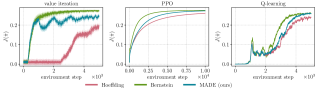
Figure 3: Performance of different count-based methods in the stochastic bidirectional lock environment. MADE performs better than the Hoeffding bonus and is comparable to the Bernstein bonus.

RL algorithms and exploration strategies.

We compare the performance of Hoeffding and Bernstein bonuses Jin et al. (2018) to MADE in three different RL algorithms. To implement MADE in tabular setting, we simply use two buffers: one that stores all past state-action pairs to estimate $\rho_{\text{cov}}$ and another one that only maintains the most recent $B$ pairs to estimate $d_{\mu}^{\pi}$. We use empirical counts to estimate both densities, which give a bonus $\propto 1/\sqrt{N_{k}(s,a)B_{k}(s,a)}$, where $N_{k}(s,a)$ is the total count and $B_{k}(s,a)$ is the recent buffer count of $(s,a)$ pair. We combine three bonuses with three RL algorithms: (1) value iteration with bonus He et al. (2020), (2) proximal policy optimization (PPO) with a model Cai et al. (2020), and (3) Q-learning with bonus Jin et al. (2018).

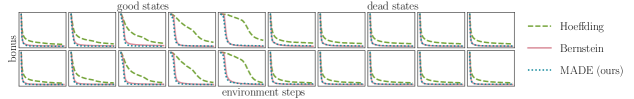
Figure 4: Values of Hoeffding, Bernstein, and MADE exploration bonus for all states and action $1$ over environment steps in the bidirectional lock MDP. MADE bonus values closely follows Bernstein bonus values.

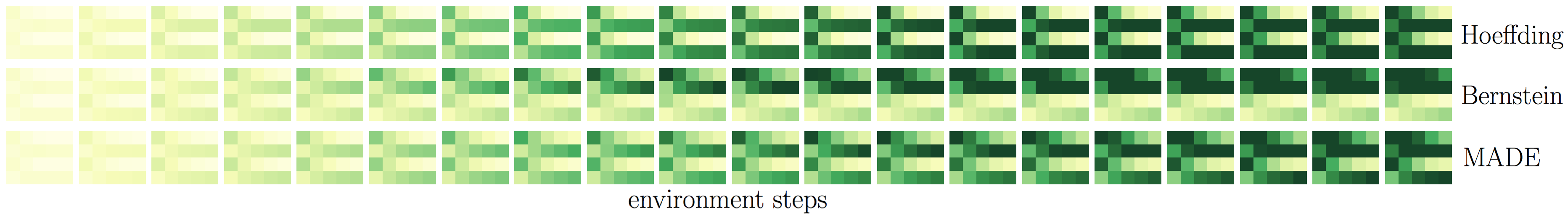
Figure 5: Heatmap of visitation counts in the bidirectional lock, plotted every $200$ iterations. The exploration strategy of MADE appears to be closet to the Bernstein bonus.

Results.

Figure 3 summarizes our results showing MADE improves over the Hoeffding bonus and is competitive to the Bernstein bonus in all three algorithms. Unlike Bernstein bonus that is hard to compute beyond tabular setting, MADE bonus design is simple and can be effectively combined with any deep RL algorithm. The experimental results suggest several interesting properties for MADE. First, MADE applies a simple modification to the Hoeffding bonus which improves the performance. Second, as illustrated in Figures 4 and 5, bonus values and exploration pattern of MADE is somewhat similar to the Bernstein bonus. This suggests that MADE may capture some structural information of the environment, similar to Bernstein bonus, which captures certain environmental properties such as the degree of stochasticity Zanette and Brunskill (2019).

4.2 Policy gradient in a chain MDP

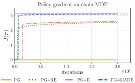
Figure 6: A deterministic chain MDP that suffers from vanishing gradients Agarwal et al. (2019). We consider a constrained tabular policy parameterization with $\pi(a|s)=\theta_{s,a}$ and $\sum_{a}\theta_{s,a}=1$. The agent always starts from $s_{0}$ and the only non-zero reward is $r(s_{H+1},a_{1})$ = 1.

We consider the chain MDP (Figure 6) presented in Agarwal et al. (2019), which suffers from vanishing gradients with policy gradient approach Sutton et al. (1999) as a positive reward is only achieved if the agent always takes action $a_{1}$. This leads to an exponential iteration complexity lower bound on the convergence of vanilla policy gradient approach even with access to exact gradients Agarwal et al. (2019). In this environment the agent always starts at state $s_{0}$ and recent guarantees on the global convergence of exact policy gradients are vacuous Bhandari and Russo (2019); Agarwal et al. (2019); Mei et al. (2020). This is because the rates depend on the ratio between the optimal and learned visitation densities, known as concentrability coefficient Kakade and Langford (2002); Scherrer (2014); Geist et al. (2017); Rashidinejad et al. (2021), or the ratio between the optimal visitation density and initial distribution Agarwal et al. (2019).

RL algorithms.

Since our goal in this experiment is to investigate the optimization effects and not exploration, we assume access to exact gradients. In this setting, we consider MADE regularizer with the form $\sum_{s,a}\sqrt{d^{\pi}(s,a)}$. Note that policy gradients take gradient of the objective with respect to the policy parameters $\theta$ and not $d^{\pi}$. We compare optimizing the policy gradient objective with four methods: vanilla version PG (e.g. uses policy gradient theorem (Williams, 1992; Sutton et al., 1999; Konda and Tsitsiklis, 2000)), relative policy entropy regularization PG+RE (Agarwal et al., 2019), policy entropy regularization PG+E (Mnih et al., 2016; Mei et al., 2020), and MADE regularization.

Results.

Figure 6 illustrates our results on policy gradient methods. As expected Agarwal et al. (2019), the vanilla version has a very slow convergence rate. Both entropy and relative entropy regularization methods are proved to achieve a linear convergence rate of $\exp(-t)$ in the iteration count $t$ Mei et al. (2020); Agarwal et al. (2019). Interestingly, MADE seems to outperforms the policy entropy regularizers, quickly converging to a globally optimal policy.

5 Experiments on MiniGrid and DeepMind Control Suite

In addition to the tabular setting, MADE can also be integrated with various model-free and model-based deep RL algorithms such as IMPALA (Espeholt et al., 2018), RAD (Lee et al., 2019a), and Dreamer (Hafner et al., 2019). As we will see shortly, MADE exploration strategy on MiniGrid (Chevalier-Boisvert et al., 2018) and DeepMind Control Suite (Tassa et al., 2020) tasks achieves state-of-the-art sample efficiency.

For a practical estimation of $\rho^{k}_{\text{cov}}$ and $d^{\pi_{\operatorname*{mix},k}}$, we adopt the two buffer idea described in the tabular setting. However, since now the state space is high-dimensional, we use RND (Burda et al., 2018b) to estimate $N_{k}(s,a)$ (and thus $\rho^{k}_{\text{cov}}$) and use a variational auto-encoder (VAE) to estimate $d^{\pi_{\operatorname*{mix},k}}$. Specifically, for RND, we minimize the difference between a predictor network $\phi^{\prime}({s,a})$ and a randomly initialized target network $\phi({s,a})$ and train it in an online manner as the agent collects data. We sample data from the recent buffer $\mathcal{B}$ to train a VAE. The length of $\mathcal{B}$ is a design choice for which we do an ablation study. Thus, the intrinsic reward in deep RL setting takes the following form

$$(1-\gamma)\tau_{k}\frac{\left\lVert\phi({s,a})-\phi^{\prime}({s,a})\right\rVert}{\sqrt{{d^{\pi_{\operatorname*{mix},k}}(s,a)}}}.$$

Model-free RL baselines.

We consider several baselines in MiniGrid: IMPALA (Espeholt et al., 2018) is a variant of policy gradient algorithms which we use as the training baseline; ICM (Pathak et al., 2017) learns a forward and reverse model for predicting state transition and uses the forward model prediction error as intrinsic reward; RND (Burda et al., 2018b) trains a predictor network to mimic a randomly initialized target network as discussed above; RIDE (Raileanu and Rocktäschel, 2020) learns a representation similar to ICM and uses the difference of learned representations along a trajectory as intrinsic reward; AMIGo (Campero et al., 2020) learns a teacher agent to assign intrinsic reward; BeBold (Zhang et al., 2020a) adopts a regulated difference of novelty measure using RND. In DeepMind Control Suite, we consider RE3 (Seo et al., 2021) as a baseline which uses a random encoder for state embedding followed by a $k$-nearest neighbour bonus for a maximum state coverage objective.

Model-based RL baselines.

MADE can be combined with model-based RL algorithms to improve sample efficiency. For baselines, we consider Dreamer, which is a well-known model-based RL algorithm for DeepMind Control Suite, as well as Dreamer+RE3, which includes RE3 bonus on top of Dreamer.

MADE achieves state-of-the-art results on both navigation and locomotion tasks by a substantial margin, greatly improving the sample efficiency of the RL exploration in both model-free and model-based methods. Further details on experiments and exact hyperparameters are provided in Appendix B.

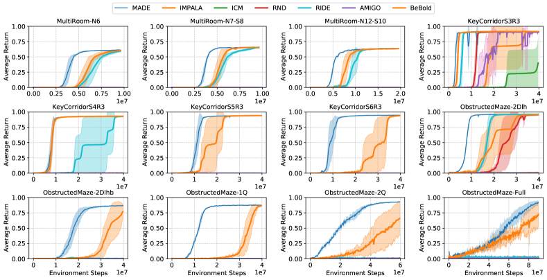
Figure 7: Results for various hard exploration tasks from MiniGrid. MADE successfully solves all the environments while other algorithms (except for BeBold) fail to solve several environments. MADE finds the optimal solution with 2-5 times fewer samples, yielding a much better sample efficiency.

5.1 Model-free RL on MiniGrid

MiniGrid (Chevalier-Boisvert et al., 2018) is a widely used benchmark for exploration in RL. Despite having symbolic states and a discrete action space, MiniGrid tasks are quite challenging. The easiest task is MultiRoom (MR) in which the agent needs to navigate to the goal by going to different rooms connected by the doors. In KeyCorridor (KC), the agent needs to search around different rooms to find the key and then use it to open the door. ObstructedMaze (OM) is a harder version of KC where the key is hidden in a box and sometimes the door is blocked by an obstruct. In addition to that, the entire environment is procedurally-generated. This adds another layer of difficulty to the problem.

From Figure 7 we can see that MADE manages to solve all the challenging tasks within 90M steps while all other baselines (except BeBold) only solve up to 50% of them. Compared to BeBold, MADE uses significantly (2-5 times) fewer samples.

5.2 Model-free RL on DeepMind Control

We also test MADE on image-based continuous control tasks of DeepMind Control Suite (Tassa et al., 2020), which is a collection of diverse control tasks such as Pendulum, Hopper, and Acrobot with realistic simulations. Compared to MiniGrid, these tasks are more realistic and complex as they involve stochastic transitions, high-dimensional states, and continuous actions. For baselines, we build our algorithm on top of RAD (Lee et al., 2019a), a strong model-free RL algorithm with a competitive sample efficiency. We compare our approach with ICM, RND, as well as RE3, which is the SOTA algorithm. Note that we compare MADE to very strong baselines. Other algorithms such as DrQ (Kostrikov et al., 2020), CURL (Srinivas et al., 2020), ProtoRL (Yarats et al., 2021), SAC+AE (Yarats et al., 2019)) perform worse based on the results reported in the original papers. MADE show consistent improvement in sample efficiency: 2.6 times over RAD+RE3, 3.3 times over RAD+RND, 19.7 times over CURL, 15.0 times over DrQ and 3.8 times over RAD.

From Figure 8, we can see that MADE consistently improves sample efficiency compared to all baselines. For these tasks, RND and ICM do not perform well and even fail on Cartpole-Swingup. RE3 achieves a comparable performance in two tasks, however, its performance on Pendulum-Swingup, Quadruped-Run, Hopper-Hop and Walker-Run is significantly worse than MADE. For example, in Pendulum-Swingup, MADE achieves a reward of around 800 in only 30K steps while RE3 requires 300k samples. In Quadruped-Run, there is a 150 reward gap between MADE and RE3, which seems to be still enlarging. These tasks show the strong performance of MADE in model-free RL.

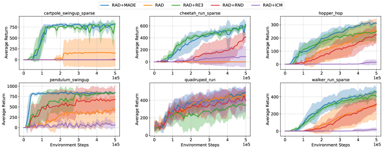
Figure 8: Results for several DeepMind control suite locomotion tasks. Comparing to all baselines, the performance of MADE is consistently better. Sometimes baseline methods even fail to solve the task.

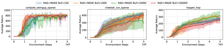
Figure 9: Ablation study on buffer size in MADE. The optimal buffer size varies in different tasks. We found buffer size of 10000 empirically works consistently reasonable.

Ablation study.

We study how the buffer length affects the performance of our algorithm in some DeepMind Control tasks. Results illustrated in Figure 9 show that for different tasks the optimal buffer length is slightly different. We empirically found that using a buffer length of 1000 consistently works well across different tasks.

5.3 Model-based RL on DeepMind Control

We also empirically verify the performance of MADE combined with the SOTA model-based RL algorithm Dreamer (Hafner et al., 2019). We compare MADE with Dreamer and Dreamer combined with RE3 in Figure 10. Results show that MADE has great sample efficiency in Cheetah-Run-Sparse, Hopper-Hop and Pendulum-Swingup environments. For example, in Hopper-Hop, MADE achieves more than 100 higher return than RE3 and 250 higher return than Dreamer, achieving a new SOTA result.

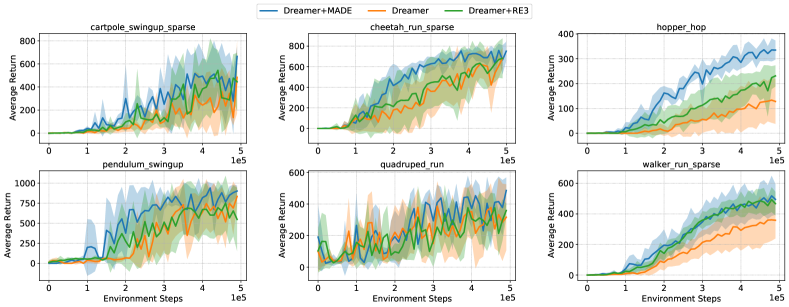
Figure 10: Results for DeepMind control suite locomotion tasks in model-based RL setting. Comparing to all baselines, the performance of MADE is consistently better. Some baseline methods even fail to solve the task.

6 Related work

Provable optimistic exploration.

Most provable exploration strategies are based on optimism in the face of uncertainty (OFU) principle. In tabular setting, model-based exploration algorithms include variants of UCB Kearns and Singh (2002); Brafman and Tennenholtz (2002), UCRL Lattimore and Hutter (2012); Jaksch et al. (2010); Zanette and Brunskill (2019); Kaufmann et al. (2021); Ménard et al. (2020), and Thompson sampling Xiong et al. (2021); Agrawal and Jia (2017); Russo (2019) and value-based methods include optimistic Q-learning Jin et al. (2018); Wang et al. (2019b); Strehl et al. (2006); Liu and Su (2020); Menard et al. (2021) and value-iteration with UCB Azar et al. (2017); Zhang et al. (2020b, c); Jin et al. (2020a). These methods are recently extended to linear MDP setting leading to a variety of model-based Zhou et al. (2020a); Ayoub et al. (2020); Jia et al. (2020); Zhou et al. (2020b), value-based Wang et al. (2019a); Jin et al. (2020b), and policy-based algorithms Cai et al. (2020); Zanette et al. (2021); Agarwal et al. (2020a). Going beyond linear function approximation, systematic exploration strategies are developed based on structural assumptions on MDP such as low Bellman rank Jiang et al. (2017) and block MDP Du et al. (2019). These methods are either computationally intractable Jiang et al. (2017); Sun et al. (2019); Ayoub et al. (2020); Zanette et al. (2020); Yang et al. (2020); Dong et al. (2021); Wang et al. (2020) or are only oracle efficient Feng et al. (2020); Agarwal et al. (2020b). The recent work Feng et al. (2021) provides a sample efficient approach with non-linear policies, however, the algorithm requires maintaining the functional form of all prior policies.

Practical exploration via intrinsic reward.

Apart from previously-discussed methods, other works give intrinsic reward based on the difference in (abstraction of) consecutive states Zhang et al. (2019); Marino et al. (2019); Raileanu and Rocktäschel (2020). However, this approach is inconsistent: the intrinsic reward does not converge to zero and thus, even with infinite samples, the final policy does not maximize the RL objective. Other intrinsic rewards try to estimate pseudo-counts Bellemare et al. (2016); Tang et al. (2017); Burda et al. (2018b, a); Ostrovski et al. (2017); Badia et al. (2020), inspired by count-only UCB bonus. Though favoring novel states, practically these methods might suffer from detachment and derailment Ecoffet et al. (2019, 2020), and forgetting Agarwal et al. (2020a). More recent works propose a combination of different criteria. RIDE (Raileanu and Rocktäschel, 2020) learns a representation via a curiosity criterion and uses the difference of consecutive states along the trajectory as the bonus. AMIGo (Campero et al., 2020) learns a teacher agent for assigning rewards for exploration. Go-Explore (Ecoffet et al., 2019) explicitly decouples the exploration and exploitation stages, yielding a more sophisticated algorithm with many hand-tuned hyperparameters.

Maximum entropy exploration.

Another line of work encourages exploration via maximizing some type of entropy. One category maximizes policy entropy Mnih et al. (2016) or relative entropy Agarwal et al. (2019) in addition to the RL objective. The work of Flet-Berliac et al. (2021) modifies the RL objective by introducing an adversarial policy which results in the next policy to move away from prior policies while staying close to the current policy. In contrast, our approach focuses on the regions explored by prior policies as opposed to the prior policies themselves. Recently, effects of policy entropy regularization have been studied theoretically Neu et al. (2017); Geist et al. (2019). In policy gradient methods with access to exact gradients, policy entropy regularization results in faster convergence by improving the optimization landscape Mei et al. (2020, 2021); Ahmed et al. (2019); Cen et al. (2020). Another category considers maximizing the entropy of state or state-action visitation densities such as Shannon entropy Hazan et al. (2019); Islam et al. (2019); Lee et al. (2019b); Seo et al. (2021) or Rényi entropy Zhang et al. (2021). Empirically, our approach achieves better performance over entropy-based methods.

Other exploration strategies.

Besides intrinsic motivation, other strategies are also fruitful in encouraging the RL agent to visit a wide range of states. One example is exploration by injecting noise to the action action space Lillicrap et al. (2015); Osband et al. (2016); Hessel et al. (2017); Osband et al. (2019) or parameter space Fortunato et al. (2018); Plappert et al. (2018). Another example is the reward-shaping category, in which diverse goals are set to guide exploration Colas et al. (2019); Florensa et al. (2018); Nair et al. (2018); Pong et al. (2020).

7 Discussion

We introduce a new exploration strategy MADE based on maximizing deviation from explored regions. We show that by simply adding a regularizer to the original RL objective, we get an easy-to-implement intrinsic reward which can be incorporated with any RL algorithm. We provide a policy computation algorithm for this objective and prove that it converges to a global optimum, provided that we have access to an approximate planner. In tabular setting, MADE consistently improves over the Hoeffding bonus and shows competitive performance to the Bernstein bonus, while the latter is impractical to compute beyond tabular. We conduct extensive experiments on MiniGrid, showing a significant (over 5 times) reduction of the required sample size. MADE also performs well in DeepMind Control Suite when combined with both model-free and model-based RL algorithms, achieving SOTA sample efficiency results. One limitation of the current work is that it only uses the naive representations of states (e.g., one-hot representation in tabular case). In fact, exploration could be conducted much more efficiently if MADE is implemented with a more compact representation of states. We leave this direction to future work.

Appendix A Convergence analysis of Algorithm 1

In this section, we provide a convergence rate analysis for Algorithm 1. Similar to Hazan et al. [2019], Algorithm 1 has access to an approximate density oracle and an approximate planner defined below:

• Visitation density oracle: We assume access to an approximate density estimator that takes in a policy $\pi$ and a density approximation error $\epsilon_{d}\geq 0$ as inputs and returns $\hat{d}^{\pi}$ such that $\|d^{\pi}-\hat{d}^{\pi}\|_{\infty}\leq\epsilon_{d}$.

• Approximate planning oracle: We assume access to an approximate planner that, given any MDP $M$ and error tolerance $\epsilon_{p}\geq 0$, returns a policy $\pi$ such that $J_{M}(\pi)\geq\max_{\pi}J_{M}(\pi)-\epsilon_{p}$.

A.1 Proof of Theorem 1

We first give the following proposition that captures certain properties of the proposed objective. The proof is postponed to the end of this section.

Proposition 1.

Consider the following regularization for $\lambda>0$

$$R_{\lambda}(d;\{d^{\pi_{i}}\}_{i=1}^{k})=\sum_{s,a}\sqrt{\frac{d(s,a)+\lambda}{\rho_{\text{cov}}(s,a)+\lambda}},$$

with $\tau_{k}=\tau/k^{c}$ where $\tau<1,c>0$. There exist constants $\beta,B,$ and $\xi$ that only depend on MDP parameters and $\lambda$ such that $L_{k}(d)\coloneqq J(d)+\tau_{k}R_{\lambda}(d;\{d^{\pi_{i}}\}_{i=1}^{k})$ satisfies the following regularity conditions for all $k\geq 1$, an appropriate choice of $c$, and valid visitation densities $d$ and $d^{\prime}$:

1. $L_{k}(d)$ is concave in $d$;

2. $L_{k}(d)$ is $\beta$-smooth: $\|\nabla L_{k}(d)-\nabla L_{k}(d^{\prime})\|_{\infty}\leq\beta\|d-d^{\prime}\|_{\infty},\quad-\beta I\preceq\nabla^{2}L_{k}(d)\preceq\beta I;$

3. $L_{k}(d)$ is $B$-bounded: $L_{k}(d)\leq B,\quad\|\nabla L_{k}(d)\|_{\infty}\leq B$;

4. There exists $\delta_{k}$ such that $\max_{d}L_{k+1}(d)-L_{k}(d)\leq\delta_{k}$ and we have $\sum_{i=0}^{k}(1-\eta)^{i}\delta_{k-i}\leq\tau\xi.$

Taking the above proposition as given for the moment, we prove Theorem 1 following steps similar to those of Hazan et al. [2019, Theorem 4.1]. By construction of the mixture density $d^{\pi_{\operatorname*{mix},k}}$, we have

$$d^{\pi_{\operatorname*{mix},k}}=(1-\eta)d^{\pi_{\operatorname*{mix},k-1}}+\eta d^{\pi_{k}}.$$

Combining the above equation with the $\beta$-smoothness of $L_{k}(d)$ yields

$$L_{k}(d^{\pi_{\operatorname*{mix},k}}) =L_{k}((1-\eta)d^{\pi_{\operatorname*{mix},k-1}}+\eta d^{\pi_{k}})$$

$$\geq L_{k}(d^{\pi_{\operatorname*{mix},k-1}})+\eta\langle d^{\pi_{k}}-d^{\pi_{\operatorname*{mix},k-1}},\nabla L_{k}(d^{\pi_{\operatorname*{mix},k-1}})\rangle-\eta^{2}\beta\|d^{\pi_{k}}-d^{\pi_{\operatorname*{mix},k-1}}\|_{2}^{2}$$

$$\geq L_{k}(d^{\pi_{\operatorname*{mix},k-1}})+\eta\langle d^{\pi_{k}}-d^{\pi_{\operatorname*{mix},k-1}},\nabla L_{k}(d^{\pi_{\operatorname*{mix},k-1}})\rangle-4\eta^{2}\beta.$$ (8)

Here the last inequality uses $\|d^{\pi_{k}}-d^{\pi_{\operatorname*{mix},k-1}}\|_{2}\leq 2$. By property (ii), we bound $\langle d^{\pi_{k}},\nabla L_{k}(d^{\pi_{\operatorname*{mix},k-1}})\rangle$ according to

$$\langle d^{\pi_{k}},\nabla L_{k}(d^{\pi_{\operatorname*{mix},k-1}})\rangle \geq\langle d^{\pi_{k}},\nabla L_{k}(\hat{d}^{\pi_{\operatorname*{mix},k-1}})\rangle-\beta\|d^{\pi_{\operatorname*{mix},k-1}}-\hat{d}^{\pi_{\operatorname*{mix},k-1}}\|_{\infty}$$

$$\geq\langle d^{\pi_{k}},\nabla L_{k}(\hat{d}^{\pi_{\operatorname*{mix},k-1}})\rangle-\beta\epsilon_{d},$$ (9)

where in the last step we used the density oracle approximation error. Recall that we defined $r_{k}=(1-\gamma)\nabla L_{k}(\hat{d}^{\pi_{\operatorname*{mix},k-1}})$. Since $\pi_{k}$ returned by the approximate planning oracle is an $\epsilon_{p}$-optimal policy in $M^{k}$, we have $(1-\gamma)^{-1}\langle d^{\pi_{k}},r_{k}\rangle\geq(1-\gamma)^{-1}\langle d^{\pi},r_{k}\rangle-\epsilon_{p}$ for any policy $\pi$, including $\pi^{\star}$. Therefore,

$$\langle d^{\pi_{k}},\nabla L_{k}(d^{\pi_{\operatorname*{mix},k-1}})\rangle \geq\langle d^{\pi^{\star}},\nabla L_{k}(\hat{d}^{\pi_{\operatorname*{mix},k-1}})\rangle-\epsilon_{p}-\beta\epsilon_{d}$$

$$\geq\langle d^{\pi^{\star}},\nabla L_{k}(d^{\pi_{\operatorname*{mix},k-1}})\rangle-\epsilon_{p}-2\beta\epsilon_{d},$$ (10)

where we used the density oracle approximation error once more in the second step. Going back to inequality (8), we further bound $L_{k}(d^{\pi_{\operatorname*{mix},k}})$ by

$$L_{k}(d^{\pi_{\operatorname*{mix},k}}) \geq L_{k}(d^{\pi_{\operatorname*{mix},k-1}})+\eta\langle d^{\pi_{k}}-d^{\pi_{\operatorname*{mix},k-1}},\nabla L_{k}(d^{\pi_{\operatorname*{mix},k-1}})\rangle-4\eta^{2}\beta$$

$$\geq L_{k}(d^{\pi_{\operatorname*{mix},k-1}})+\eta\langle d^{\pi^{\star}}-d^{\pi_{\operatorname*{mix},k-1}},\nabla L_{k}(d^{\pi_{\operatorname*{mix},k-1}})\rangle-\eta\epsilon_{p}-2\eta\beta\epsilon_{d}-4\eta^{2}\beta$$

$$\geq(1-\eta)L_{k}(d^{\pi_{\operatorname*{mix},k-1}})+\eta L_{k}(d^{\pi^{\star}})-4\eta^{2}\beta-\eta\epsilon_{p}-2\eta\beta\epsilon_{d},$$

where the last inequality is by concavity of $L_{k}(d)$. Therefore,

$$L_{k}(d^{\pi^{\star}})-L_{k}(d^{\pi_{\operatorname*{mix},k}})\leq(1-\eta)[L_{k}(d^{\pi^{\star}})-L_{k}(d^{\pi_{\operatorname*{mix},k-1}})]+2\eta\beta\epsilon_{d}+\eta\epsilon_{p}+4\eta^{2}\beta.$$

By assumption (iv), we write

$$L_{K+1}(d^{\pi^{\star}})-L_{K+1}(d^{\pi_{\operatorname*{mix},K}}) \leq L_{K}(d^{\pi^{\star}})-L_{K}(d^{\pi_{\operatorname*{mix},K}})+2\delta_{K}$$

$$\leq(1-\eta)[L_{K}(d^{\pi^{\star}})-L_{K}(d^{\pi_{\operatorname*{mix},K-1}})]+2\delta_{K}+2\eta\beta\epsilon_{d}+\eta\epsilon_{p}+4\eta^{2}\beta$$

$$\leq Be^{-\eta K}+2\beta\epsilon_{d}+\epsilon_{p}+4\eta\beta+2\sum_{i=0}^{K}(1-\eta)^{i}\delta_{K-i}$$

$$\leq Be^{-\eta K}+2\beta\epsilon_{d}+\epsilon_{p}+4\eta\beta+2\tau\xi.$$

It is straightforward to check that setting $\eta\leq 0.1\epsilon\beta^{-1},\epsilon_{p}\leq 0.1\epsilon,\epsilon_{d}\leq 0.1\epsilon\beta^{-1},\tau\leq 0.1\epsilon,$ and the number of iterations $K\geq\eta^{-1}\log(10B\epsilon^{-1})$ yields the claim of Theorem 1.

Remark 2.

Since the temperature parameter $\tau_{k}$ in Proposition 1 goes to zero as $k$ increases, one can show that the expected value of policy returned by Algorithm 1 converges to the maximum performance $J(\pi^{\star})$.

Proof of Proposition 1..

For claim (ii), observe that $\nabla^{2}L_{k}(d)$ is a diagonal matrix whose $(s,a)$ diagonal term is given by

$$(\nabla^{2}L_{k}(d))_{s,a}=\frac{-\tau}{4k^{c}}\times\frac{1}{(d(s,a)+\lambda)^{3/2}(\rho_{\text{cov}}(s,a)+\lambda)^{1/2}}.$$

The diagonal elements are bounded by $-1/(4\lambda^{2})\leq(\nabla^{2}L_{k}(d))_{s,a}\leq\frac{1}{4\lambda^{2}}=:\beta$. Furthermore, by Taylor’s theorem, one has

$$\|\nabla L_{k}(d)-\nabla L_{k}(d^{\prime})\|_{\infty}\leq\max_{(s,a),\alpha\in[0,1]}(\nabla^{2}L_{k}(\alpha d+(1-\alpha)d^{\prime}))\|d-d^{\prime}\|_{\infty}\leq\beta\|d-d^{\prime}\|_{\infty}.$$

Claim (i) is immediate from the above calculation as the Hessian $\nabla^{2}L_{k}(d)$ is negative definite. Claim (iii) may be verified by explicit calculation:

$$\sum_{s,a}d(s,a)r(s,a)+\frac{\tau}{k^{c}}\sum_{s,a}\sqrt{\frac{d(s,a)+\lambda}{\rho_{\text{cov}}(s,a)+\lambda}}\leq SA\left(1+\sqrt{\frac{1+\lambda}{\lambda}}\right)=:B.$$

For claim (iv), we have

$$L_{k+1}(d)-L_{k}(d)\leq\sum_{s,a}\frac{\tau}{(k+1)^{c}}\sqrt{\frac{d(s,a)+\lambda}{\rho_{\text{cov}}(s,a)+\lambda}}\leq\frac{SA\tau}{(k+1)^{c}}\sqrt{\frac{1+\lambda}{\lambda}}=:\delta_{k}$$

We have

$$\sum_{i=0}^{k}(1-\eta)^{i}\delta_{k-i}=\tau SA\sqrt{\frac{1+\lambda}{\lambda}}\sum_{i=0}^{k}\frac{(1-\eta)^{i}}{(k-i+1)^{c}}.$$

For example, for $c=2$, the above sum is bounded by $\sum_{n=1}^{\infty}1/n^{2}=\pi^{2}/6$. Thus, one can set $\xi\coloneqq\frac{\pi^{2}SA}{6}\sqrt{\frac{1+\lambda}{\lambda}}$. ∎

Appendix B Experimental details

Source code is included in the supplemental material.

B.1 Bidirectional lock

Environment.

For the bidirectional lock environment, one of the locks (randomly chosen) gives a larger reward of $1$ and the other lock gives a reward of $0.1$. Further details on this environment can be found in the work Agarwal et al. [2020a].

Exploration bonuses.

We consider three exploration bonuses:

• Hoeffding-style bonus is equal to

  $$\frac{V_{\max}}{\sqrt{N_{k}(s,a)}},$$

  for every $s\in\mathcal{S},a\in\mathcal{A}$, where $V_{\max}$ is the maximum possible value in an environment which we set to 1 for bidirectional lock.

• We use a Bernstein-style bonus

  $$\sqrt{\frac{\text{Var}_{s^{\prime}\sim P_{k}(\cdot\mid s,a)}V_{k}(s^{\prime})}{N_{k}(s,a)}}+\frac{1}{N_{k}(s,a)}$$

  based on the bonus proposed by He et al. [2020]. $P_{k}$ denotes an empirical estimation of transitions $P_{k}(s^{\prime}|s,a)=N_{k}(s,a,s^{\prime})/N_{k}(s,a)$, where $N_{k}(s,a,s^{\prime})$ is the number of samples on transiting to $s^{\prime}$ starting from state $s$ and taking action $a$.

• MADE’s bonus is set to the following in tabular setting:

  $$\frac{1}{\sqrt{N_{k}(s,a)B_{k}(s,a)}}.$$

Algorithms.

Below, we describe details on each tabular algorithm.

• Value iteration. We implement discounted value iteration given in He et al. [2020] with all three bonuses.

• PPO. We implement a tabular version of the algorithm in Cai et al. [2020], which is based on PPO with bonus. Specifically, the algorithm has the following steps: (1) sampling a new trajectory by running the stochastic policy $\pi_{k}$, (2) updating the empirical transition estimate $P_{k}$ and exploration bonus, (3) computing Q-function $Q_{k}$ of $\pi_{k}$ over an MDP $M_{k}$ with empirical transitions $P_{k}$ and total reward $r_{k}$ which is a sum of extrinsic reward and exploration bonus, and (4) updating the policy according to $\pi_{k+1}(a|s)\propto\pi_{k}(a|s)\exp(\alpha_{k}Q_{k}(s,a))$, where $\alpha_{k}=\sqrt{2\log(A)/HK}$ based on Cai et al. [2020, Theorem 13.1].

• Q-learning. We implement Q-learning with bonus based on the algorithms given by Jin et al. [2018].

B.2 Chain MDP

For the chain MDP described in Section 4.2, we use $H=8$ and discount factor $\gamma=H/(H+1)$. We run policy gradient for a tabular softmax policy parameterization $\pi(s|a)=\theta_{s,a}$ with the following RL objectives. Since we use a simplex parameterization, we run projected gradient ascent.

• Vanilla PG. The vanilla version simply considers the standard RL objective $J(\pi_{\theta})$. For the gradient $\nabla_{\theta}J(\pi_{\theta})$, see e.g. Agarwal et al. [2019, Equation (32)].

• PG with relative policy entropy regularization. We use the objective (with the additive constant dropped) given in Agarwal et al. [2019, Equation (12)]:

  $$L(\pi_{\theta})\coloneqq J(\pi_{\theta})+\tau_{k}\sum_{s,a}\log\pi_{\theta}(a|s).$$

  Here, index $k$ denotes the policy gradient step. This form of regularization is more aggressive than the policy entropy regularized objective discussed next. Partial derivatives of the above objective are simply

  $$\frac{\partial L(\pi_{\theta})}{\partial\theta_{s,a}}=\frac{\partial J(\pi_{\theta})}{\partial\theta_{s,a}}+\tau_{k}\frac{1}{\theta_{s,a}},$$

  where the first term is analogous to the vanilla policy gradient.

• PG with policy entropy regularization. Policy entropy regularized objective Williams and Peng [1991], Mnih et al. [2016], Nachum et al. [2017], Mei et al. [2020] is

  $$L(\pi_{\theta})\coloneqq J(\pi_{\theta})-\tau_{k}(1-\gamma)^{-1}\operatorname{\mathbb{E}}_{(s,a)\sim d^{\pi_{\theta}}_{\rho}(\cdot,\cdot)}[\log\pi_{\theta}(a|s)].$$

  The gradient of the regularizer of the above objective is given in Lemma 1.

• PG with MADE’s regularization. For MADE, we use the following objective

  $$L(\pi_{\theta})\coloneqq J(\pi_{\theta})-\tau_{k}\sum_{s,a}\sqrt{d^{\pi}(s,a)}.$$

  The gradient of MADE’s regularizer is computed in Lemma 2.

For all regularized objectives, we set $\tau_{k}=0.1/\sqrt{k}$.

B.3 MiniGrid

We follow RIDE [Campero et al., 2020] and use the same hyperparameters for all the baselines. For ICM, RND, IMPALA, RIDE, BeBold and MADE, we use the learning rate $10^{-4}$, batch size $32$, unroll length $100$, RMSProp optimizer with $\epsilon=0.01$ and momentum $0$. For entropy cost hyperparameters, we use 0.0005 for all the baselines except AMIGo. We provide the entropy cost for AMIGo below. We also test different values $\{0.01,0.02,0.05,0.1,0.5\}$ for the temperature hyperparameter in MADE. The best hyperparameters we found for each method are as follows. For Bebold, RND, and MADE we use intrinsic reward scaling factor of 0.1 for all environments. For ICM we use intrinsic reward scaling factor of 0.1 for KeyCorridor environments and 0.5 for the others. Hyperparameters in RIDE are exactly the same as ICM. For AMIGo, we use an entropy cost of $0.0005$ for the student agent, and an entropy cost of $0.01$ for the teacher agent.

B.4 DeepMind Control Suite

Environment.

We use the publicly available environment DeepMind Control Suite [Tassa et al., 2020] without any modification (Figure 11). Following the task design of RE3 [Seo et al., 2021], we use Cheetah_Run_Sparse and Walker_Run_Sparse.

Figure 11: Visualization of various tasks in DeepMind Control Suite. DeepMind Control Suite includes image-based control tasks with physics simulation. We mainly experiment on locomotion tasks in this environment.

Model-free RL implementations.

For the experiments, we use the baselines of RAD [Laskin et al., 2020], and we conduct a hyperparameter search over certain factors:

• RND. We search for the temperature parameter $\tau_{k}$ over $\{0.001,0.01,0.05,0.1,0.5,10.0\}$ and choose the best for each task. Specifically we use $\tau_{k}=0.1$ for Pendulum_Swingup and
  Cheetah_Run_Sparse, $\tau_{k}=10$ for Cartpole_Swingup_Sparse, and $\tau_{k}=0.05$ for others.

• ICM. We search for the temperature parameter $\tau_{k}$ over $\{0.001,0.01,0.05,0.1,0.5,1.0\}$ and choose the best for each task. Specifically we select $\tau_{k}=1.0$ for Cheetah_Run_Sparse and $\tau_{k}=0.1$ for the others. For the total loss used in training the networks, to balance the coefficient between forward loss and inverse loss, we follow the convention and use $L_{\mathrm{all}}=0.2\cdot L_{\mathrm{forward}}+0.8\cdot L_{\mathrm{inverse}}$, where $L_{\mathrm{forward}}$ is the loss of predicting the next state given current state-action pair and $L_{\mathrm{inverse}}$ is the loss for predicting the action given the current state and the next state.

• RE3. We use an initial scaling factor $\tau_{0}=0.05$ (the scaling factor of $\tau_{k}$ at step 0) and decay it afterwards in each step. Note that we use the number of clusters $M=3$ with a decaying factor on the reward $\rho=\{0.00001,0.000025\}$. Therefore, the final intrinsic reward scaling factor becomes: $\tau_{k}=\tau_{0}e^{-\rho k}$.

• MADE. We search for the temperature parameter $\tau_{k}$ over $\{0.001,0.01,0.05,0.1,0.5\}$ and choose the best for each task. Specifically we select $\tau_{k}=0.05$ for Cartpole_Swingup_Sparse,
  Walker_Run_Sparse and Cheetah_Run_Sparse, $\tau_{k}=0.5$ for Hopper_Hop and Pendulum_Swingup, and $\tau_{k}=0.001$ for Quadruped_Run.

We use the same network architecture for all the algorithms. Specifically, the encoder consists of 4 convolution layers with ReLU activations. There are kernels of size 3 × 3 with 32 channels for all layers, and stride 1 except for the first layer which has stride 2. The embedding is then followed by a LayerNorm.

Model-based Rl implementation

Here we provide implementation details for the model-based RL experiments. We adopt Dreamer as a baseline and build all the algorithms on top of that.

• RE3. For RE3, we follow the hyperparameters given in the original paper. We use an initial scaling factor $\tau_{0}=0.1$ without decaying $\tau_{k}$ afterwards. The number of clusters is set to $M=50$. We use a decaying factor on the reward $\rho=0$.

• MADE. We search for the temperature parameter $\tau_{k}$ over $\{0.0005,0.01,0.05,0.1,0.5\}$ and choose the best for each map. Specifically we use 0.5 for Cartpole_Swingup_Sparse, Cheetah_Run_Sparse and Hopper_Hop, 0.01 for Walker_Run_Sparse and Pendulum_Swingup and 0.0005 for Quadruped_Run.

Appendix C Gradient computations

In this section we compute the gradients for policy entropy and MADE regularizers used in the chain MDP experiment. Before presenting the lemmas, we define two other visitation densities. The state visitation density $d^{\pi}:\mathcal{S}\rightarrow[0,1]$ is defined as

$$d^{\pi}(s)\coloneqq(1-\gamma)\sum_{t=0}^{\infty}\gamma^{t}\operatorname{\mathbb{P}}_{t}(s_{t}=s;\pi),$$

where $\operatorname{\mathbb{P}}_{t}(s_{t}=s;\pi)$ denotes the probability of visiting $s$ at step $t$ starting at $s_{0}\sim\rho(\cdot)$ following policy $\pi$. The state-action visitation density starting at $(s^{\prime},a^{\prime})$ is denoted by

$$d^{\pi}_{s^{\prime},a^{\prime}}(s,a)\coloneqq(1-\gamma)\sum_{t=0}^{\infty}\gamma^{t}\operatorname{\mathbb{P}}_{t}(s_{t}=s,a_{t}=a;\pi,s_{0}=s^{\prime},a_{0}=a^{\prime}).$$

The following lemma computes the gradient of policy entropy with respect to policy parameters.

Lemma 1.

For a policy $\pi$ parameterized by $\theta$, the gradient of the policy entropy

$$R(\pi_{\theta})\coloneqq-\operatorname{\mathbb{E}}_{(s,a)\sim d^{\pi_{\theta}}_{\rho}(\cdot,\cdot)}[\log\pi_{\theta}(a|s)],$$

with respect to $\theta$ is given by

$$\nabla_{\theta}R(\pi_{\theta})=\operatorname{\mathbb{E}}_{(s,a)\sim d^{\pi_{\theta}}_{\rho}(\cdot,\cdot)}\left[\nabla_{\theta}\log\pi(a|s)\left(\frac{1}{1-\gamma}\langle d^{\pi}_{s,a},-\log\pi\rangle\right)-\log\pi(a|s)\right].$$

Proof.

By chain rule, we write

$$\nabla_{\theta}R(\pi_{\theta})=-\sum_{s,a}\nabla_{\theta}d^{\pi}(s,a)\log\pi(a|s)+\sum_{s,a}d^{\pi}(s,a)\nabla_{\theta}\log\pi(a|s)=-\sum_{s,a}\nabla_{\theta}d^{\pi}(s,a)\log\pi(a|s).$$

The second equation uses the fact that $\operatorname{\mathbb{E}}_{x\sim p(\cdot)}[\nabla_{\theta}\log p(x)]=0$ for any density $p$ and that $d^{\pi}(s,a)=d^{\pi}(s)\pi(a|s)$ as laid out below:

$$\sum_{s,a}d^{\pi}(s,a)\nabla_{\theta}\log\pi(a|s)=\sum_{s}d^{\pi}(s)\sum_{a}\pi(a|s)\nabla_{\theta}\log\pi(a|s)=0.$$

By another application of chain rule, one can write

$$\nabla_{\theta}d^{\pi}(s,a)=\nabla_{\theta}[d^{\pi}(s)\pi(a|s)]=\nabla_{\theta}d^{\pi}(s)\pi(a|s)+d^{\pi}(s,a)\nabla_{\theta}\log\pi(a|s).$$

We further simplify $\nabla_{\theta}R(\pi_{\theta})$ according to

$$\nabla_{\theta}R(\pi_{\theta}) =-\sum_{s,a}\nabla_{\theta}d^{\pi}(s,a)\log\pi(a|s)$$

$$=-\sum_{s,a}\nabla_{\theta}d^{\pi}(s)\pi(a|s)\log\pi(a|s)-\sum_{s,a}d^{\pi}(s,a)\nabla_{\theta}\log\pi(a|s)\log\pi(a|s).$$

We substitute $\nabla_{\theta}d^{\pi}(s)$ based on Zhang et al. [2021, Lemma D.1]:

$$\nabla_{\theta}R(\pi_{\theta})= -\frac{1}{1-\gamma}\sum_{s^{\prime},a^{\prime}}d^{\pi}(s^{\prime},a^{\prime})\nabla_{\theta}\log(a^{\prime}|s^{\prime})\sum_{s,a}d_{s^{\prime},a^{\prime}}(s,a)\log\pi(a|s)$$

$$\quad-\sum_{s,a}d^{\pi}(s,a)\nabla_{\theta}\log\pi(a|s)\log\pi(a|s)$$

$$= \operatorname{\mathbb{E}}_{(s,a)\sim d^{\pi_{\theta}}_{\rho}(\cdot,\cdot)}\left[\nabla_{\theta}\log\pi(a|s)\left(\frac{1}{1-\gamma}\langle d^{\pi}_{s,a},-\log\pi\rangle\right)-\log\pi(a|s)\right],$$

where $\langle d^{\pi}_{s,a},-\log\pi\rangle$ denotes the inner product between vectors $d^{\pi}_{s,a}$ and $-\log\pi$. This completes the proof. ∎

The following lemma computes the gradient of MADE regularizer with respect to policy parameters.

Lemma 2.

For a policy $\pi$ parameterized by $\theta$, the gradient of the regularizer

$$R(\pi_{\theta})\coloneqq\sum_{s,a}\sqrt{d^{\pi}(s,a)},$$

with respect to $\theta$ is given by

$$\nabla_{\theta}R(\pi_{\theta})=\frac{1}{2}\operatorname{\mathbb{E}}_{(s,a)\sim d^{\pi}(\cdot,\cdot)}\left[\nabla_{\theta}\log\pi(a|s)\left(\frac{1}{1-\gamma}\langle d^{\pi}_{s,a},\frac{1}{\sqrt{d^{\pi}}}\rangle+\frac{1}{\sqrt{d^{\pi}(s,a)}}\right)\right].$$

Proof.

The proof is similar to that of Zhang et al. [2021, Lemma D.3]. We write $\nabla_{\theta}d^{\pi}(s,a)=\nabla_{\theta}d^{\pi}(s)\pi(a|s)+d^{\pi}(s,a)\nabla_{\theta}\log\pi(a|s)$ and conclude based on Zhang et al. [2021, Lemma D.1] that

$$\nabla_{\theta}R(\pi_{\theta})= \frac{1}{2}\sum_{s,a}\frac{\nabla_{\theta}d^{\pi}(s,a)}{\sqrt{d^{\pi}(s,a)}}$$

$$= \frac{1}{2(1-\gamma)}\sum_{s^{\prime},a^{\prime}}d^{\pi}(s^{\prime},a^{\prime})\nabla_{\theta}\log\pi(a^{\prime}|s^{\prime})\sum_{s,a}d^{\pi}_{s^{\prime},a^{\prime}}(s,a)\frac{1}{\sqrt{d^{\pi}(s,a)}}$$

$$\quad+\frac{1}{2}\sum_{s,a}d^{\pi}(s,a)\nabla_{\theta}\log\pi(a|s)\frac{1}{\sqrt{d^{\pi}(s,a)}}$$

$$= \frac{1}{2}\operatorname{\mathbb{E}}_{(s,a)\sim d^{\pi}(\cdot,\cdot)}\left[\nabla_{\theta}\log\pi(a|s)\left(\frac{1}{1-\gamma}\langle d^{\pi}_{s,a},\frac{1}{\sqrt{d^{\pi}}}\rangle+\frac{1}{\sqrt{d^{\pi}(s,a)}}\right)\right].$$

∎

References

- Agarwal et al. [2019] Alekh Agarwal, Sham M Kakade, Jason D Lee, and Gaurav Mahajan. On the theory of policy gradient methods: Optimality, approximation, and distribution shift. arXiv preprint arXiv:1908.00261, 2019.
- Agarwal et al. [2020a] Alekh Agarwal, Mikael Henaff, Sham Kakade, and Wen Sun. PC-PG: Policy cover directed exploration for provable policy gradient learning. arXiv preprint arXiv:2007.08459, 2020a.
- Agarwal et al. [2020b] Alekh Agarwal, Sham Kakade, Akshay Krishnamurthy, and Wen Sun. Flambe: Structural complexity and representation learning of low rank MDPs. arXiv preprint arXiv:2006.10814, 2020b.
- Agrawal and Jia [2017] Shipra Agrawal and Randy Jia. Optimistic posterior sampling for reinforcement learning: Worst-case regret bounds. In Proceedings of the 31st International Conference on Neural Information Processing Systems, pages 1184–1194, 2017.
- Ahmed et al. [2019] Zafarali Ahmed, Nicolas Le Roux, Mohammad Norouzi, and Dale Schuurmans. Understanding the impact of entropy on policy optimization. In International Conference on Machine Learning, pages 151–160. PMLR, 2019.
- Ayoub et al. [2020] Alex Ayoub, Zeyu Jia, Csaba Szepesvari, Mengdi Wang, and Lin Yang. Model-based reinforcement learning with value-targeted regression. In International Conference on Machine Learning, pages 463–474. PMLR, 2020.
- Azar et al. [2017] Mohammad Gheshlaghi Azar, Ian Osband, and Rémi Munos. Minimax regret bounds for reinforcement learning. In International Conference on Machine Learning, pages 263–272. PMLR, 2017.
- Badia et al. [2020] Adrià Puigdomènech Badia, Pablo Sprechmann, Alex Vitvitskyi, Daniel Guo, Bilal Piot, Steven Kapturowski, Olivier Tieleman, Martín Arjovsky, Alexander Pritzel, Andew Bolt, et al. Never give up: Learning directed exploration strategies. arXiv preprint arXiv:2002.06038, 2020.
- Bellemare et al. [2016] Marc Bellemare, Sriram Srinivasan, Georg Ostrovski, Tom Schaul, David Saxton, and Remi Munos. Unifying count-based exploration and intrinsic motivation. In Advances in neural information processing systems, pages 1471–1479, 2016.
- Bhandari and Russo [2019] Jalaj Bhandari and Daniel Russo. Global optimality guarantees for policy gradient methods. arXiv preprint arXiv:1906.01786, 2019.
- Brafman and Tennenholtz [2002] Ronen I Brafman and Moshe Tennenholtz. R-max: A general polynomial time algorithm for near-optimal reinforcement learning. Journal of Machine Learning Research, 3(Oct):213–231, 2002.
- Brockman et al. [2016] Greg Brockman, Vicki Cheung, Ludwig Pettersson, Jonas Schneider, John Schulman, Jie Tang, and Wojciech Zaremba. Openai gym. arXiv preprint arXiv:1606.01540, 2016.
- Burda et al. [2018a] Yuri Burda, Harri Edwards, Deepak Pathak, Amos Storkey, Trevor Darrell, and Alexei A Efros. Large-scale study of curiosity-driven learning. arXiv preprint arXiv:1808.04355, 2018a.
- Burda et al. [2018b] Yuri Burda, Harrison Edwards, Amos Storkey, and Oleg Klimov. Exploration by random network distillation. arXiv preprint arXiv:1810.12894, 2018b.
- Cai et al. [2020] Qi Cai, Zhuoran Yang, Chi Jin, and Zhaoran Wang. Provably efficient exploration in policy optimization. In International Conference on Machine Learning, pages 1283–1294. PMLR, 2020.
- Campero et al. [2020] Andres Campero, Roberta Raileanu, Heinrich Küttler, Joshua B Tenenbaum, Tim Rocktäschel, and Edward Grefenstette. Learning with AMIGo: Adversarially motivated intrinsic goals. arXiv preprint arXiv:2006.12122, 2020.
- Cen et al. [2020] Shicong Cen, Chen Cheng, Yuxin Chen, Yuting Wei, and Yuejie Chi. Fast global convergence of natural policy gradient methods with entropy regularization. arXiv preprint arXiv:2007.06558, 2020.
- Chevalier-Boisvert et al. [2018] Maxime Chevalier-Boisvert, Lucas Willems, and Suman Pal. Minimalistic gridworld environment for OpenAI Gym. https://github.com/maximecb/gym-minigrid, 2018.
- Colas et al. [2019] Cédric Colas, Pierre Fournier, Mohamed Chetouani, Olivier Sigaud, and Pierre-Yves Oudeyer. CURIOUS: Intrinsically motivated modular multi-goal reinforcement learning. In International conference on machine learning, pages 1331–1340. PMLR, 2019.
- Dong et al. [2021] Kefan Dong, Jiaqi Yang, and Tengyu Ma. Provable model-based nonlinear bandit and reinforcement learning: Shelve optimism, embrace virtual curvature. arXiv preprint arXiv:2102.04168, 2021.
- Du et al. [2019] Simon Du, Akshay Krishnamurthy, Nan Jiang, Alekh Agarwal, Miroslav Dudik, and John Langford. Provably efficient RL with rich observations via latent state decoding. In International Conference on Machine Learning, pages 1665–1674. PMLR, 2019.
- Ecoffet et al. [2019] Adrien Ecoffet, Joost Huizinga, Joel Lehman, Kenneth O Stanley, and Jeff Clune. Go-explore: A new approach for hard-exploration problems. arXiv preprint arXiv:1901.10995, 2019.
- Ecoffet et al. [2020] Adrien Ecoffet, Joost Huizinga, Joel Lehman, Kenneth O Stanley, and Jeff Clune. First return then explore. arXiv preprint arXiv:2004.12919, 2020.
- Espeholt et al. [2018] Lasse Espeholt, Hubert Soyer, Remi Munos, Karen Simonyan, Volodymir Mnih, Tom Ward, Yotam Doron, Vlad Firoiu, Tim Harley, Iain Dunning, et al. Impala: Scalable distributed deep-RL with importance weighted actor-learner architectures. arXiv preprint arXiv:1802.01561, 2018.
- Feng et al. [2020] Fei Feng, Ruosong Wang, Wotao Yin, Simon S Du, and Lin Yang. Provably efficient exploration for reinforcement learning using unsupervised learning. Advances in Neural Information Processing Systems, 33, 2020.
- Feng et al. [2021] Fei Feng, Wotao Yin, Alekh Agarwal, and Lin F Yang. Provably correct optimization and exploration with non-linear policies. arXiv preprint arXiv:2103.11559, 2021.
- Flet-Berliac et al. [2021] Yannis Flet-Berliac, Johan Ferret, Olivier Pietquin, Philippe Preux, and Matthieu Geist. Adversarially guided actor-critic. In International Conference on Learning Representations, 2021.
- Florensa et al. [2018] Carlos Florensa, David Held, Xinyang Geng, and Pieter Abbeel. Automatic goal generation for reinforcement learning agents. In International conference on machine learning, pages 1515–1528. PMLR, 2018.
- Fortunato et al. [2018] Meire Fortunato, Mohammad Gheshlaghi Azar, Bilal Piot, Jacob Menick, Ian Osband, Alex Graves, Vlad Mnih, Remi Munos, Demis Hassabis, Olivier Pietquin, et al. Noisy networks for exploration. International Conference on Learning Representations, 2018.
- Geist et al. [2017] Matthieu Geist, Bilal Piot, and Olivier Pietquin. Is the Bellman residual a bad proxy? In Proceedings of the 31st International Conference on Neural Information Processing Systems, pages 3208–3217, 2017.
- Geist et al. [2019] Matthieu Geist, Bruno Scherrer, and Olivier Pietquin. A theory of regularized Markov decision processes. In International Conference on Machine Learning, pages 2160–2169. PMLR, 2019.
- Gregor et al. [2016] Karol Gregor, Danilo Jimenez Rezende, and Daan Wierstra. Variational intrinsic control. arXiv preprint arXiv:1611.07507, 2016.
- Hafner et al. [2019] Danijar Hafner, Timothy Lillicrap, Jimmy Ba, and Mohammad Norouzi. Dream to control: Learning behaviors by latent imagination. arXiv preprint arXiv:1912.01603, 2019.
- Hazan et al. [2019] Elad Hazan, Sham Kakade, Karan Singh, and Abby Van Soest. Provably efficient maximum entropy exploration. In International Conference on Machine Learning, pages 2681–2691, 2019.
- He et al. [2020] Jiafan He, Dongruo Zhou, and Quanquan Gu. Nearly minimax optimal reinforcement learning for discounted MDPs. arXiv preprint arXiv:2010.00587, 2020.
- Hessel et al. [2017] Matteo Hessel, Joseph Modayil, Hado Van Hasselt, Tom Schaul, Georg Ostrovski, Will Dabney, Dan Horgan, Bilal Piot, Mohammad Azar, and David Silver. Rainbow: Combining improvements in deep reinforcement learning. arXiv preprint arXiv:1710.02298, 2017.
- Islam et al. [2019] Riashat Islam, Zafarali Ahmed, and Doina Precup. Marginalized state distribution entropy regularization in policy optimization. arXiv preprint arXiv:1912.05128, 2019.
- Jaksch et al. [2010] Thomas Jaksch, Ronald Ortner, and Peter Auer. Near-optimal regret bounds for reinforcement learning. Journal of Machine Learning Research, 11(4), 2010.
- Jia et al. [2020] Zeyu Jia, Lin Yang, Csaba Szepesvari, and Mengdi Wang. Model-based reinforcement learning with value-targeted regression. In Learning for Dynamics and Control, pages 666–686. PMLR, 2020.
- Jiang et al. [2017] Nan Jiang, Akshay Krishnamurthy, Alekh Agarwal, John Langford, and Robert E Schapire. Contextual decision processes with low Bellman rank are PAC-learnable. In International Conference on Machine Learning, pages 1704–1713. PMLR, 2017.
- Jin et al. [2018] Chi Jin, Zeyuan Allen-Zhu, Sebastien Bubeck, and Michael I Jordan. Is Q-learning provably efficient? In Proceedings of the 32nd International Conference on Neural Information Processing Systems, pages 4868–4878, 2018.
- Jin et al. [2020a] Chi Jin, Akshay Krishnamurthy, Max Simchowitz, and Tiancheng Yu. Reward-free exploration for reinforcement learning. In International Conference on Machine Learning, pages 4870–4879. PMLR, 2020a.
- Jin et al. [2020b] Chi Jin, Zhuoran Yang, Zhaoran Wang, and Michael I Jordan. Provably efficient reinforcement learning with linear function approximation. In Conference on Learning Theory, pages 2137–2143. PMLR, 2020b.
- Kakade and Langford [2002] Sham Kakade and John Langford. Approximately optimal approximate reinforcement learning. In In Proc. 19th International Conference on Machine Learning. Citeseer, 2002.
- Kakade et al. [2018] Sham Kakade, Mengdi Wang, and Lin F Yang. Variance reduction methods for sublinear reinforcement learning. arXiv preprint arXiv:1802.09184, 2018.
- Kaufmann et al. [2021] Emilie Kaufmann, Pierre Ménard, Omar Darwiche Domingues, Anders Jonsson, Edouard Leurent, and Michal Valko. Adaptive reward-free exploration. In Algorithmic Learning Theory, pages 865–891. PMLR, 2021.
- Kearns and Singh [2002] Michael Kearns and Satinder Singh. Near-optimal reinforcement learning in polynomial time. Machine learning, 49(2):209–232, 2002.
- Kim et al. [2018] Hyoungseok Kim, Jaekyeom Kim, Yeonwoo Jeong, Sergey Levine, and Hyun Oh Song. Emi: Exploration with mutual information. arXiv preprint arXiv:1810.01176, 2018.
- Klyubin et al. [2005] Alexander S Klyubin, Daniel Polani, and Chrystopher L Nehaniv. All else being equal be empowered. In European Conference on Artificial Life, pages 744–753. Springer, 2005.
- Konda and Tsitsiklis [2000] Vijay R Konda and John N Tsitsiklis. Actor-critic algorithms. In Advances in neural information processing systems, pages 1008–1014. Citeseer, 2000.
- Kostrikov et al. [2020] Ilya Kostrikov, Denis Yarats, and Rob Fergus. Image augmentation is all you need: Regularizing deep reinforcement learning from pixels. arXiv preprint arXiv:2004.13649, 2020.
- Laskin et al. [2020] Michael Laskin, Kimin Lee, Adam Stooke, Lerrel Pinto, Pieter Abbeel, and Aravind Srinivas. Reinforcement learning with augmented data. arXiv preprint arXiv:2004.14990, 2020.
- Lattimore and Hutter [2012] Tor Lattimore and Marcus Hutter. PAC bounds for discounted MDPs. In International Conference on Algorithmic Learning Theory, pages 320–334. Springer, 2012.
- Lee et al. [2019a] Kimin Lee, Kibok Lee, Jinwoo Shin, and Honglak Lee. Network randomization: A simple technique for generalization in deep reinforcement learning. arXiv preprint arXiv:1910.05396, 2019a.
- Lee et al. [2019b] Lisa Lee, Benjamin Eysenbach, Emilio Parisotto, Eric Xing, Sergey Levine, and Ruslan Salakhutdinov. Efficient exploration via state marginal matching. arXiv preprint arXiv:1906.05274, 2019b.
- Lillicrap et al. [2015] Timothy P Lillicrap, Jonathan J Hunt, Alexander Pritzel, Nicolas Heess, Tom Erez, Yuval Tassa, David Silver, and Daan Wierstra. Continuous control with deep reinforcement learning. arXiv preprint arXiv:1509.02971, 2015.
- Liu and Su [2020] Shuang Liu and Hao Su. Regret bounds for discounted MDPs. arXiv preprint arXiv:2002.05138, 2020.
- Marino et al. [2019] Kenneth Marino, Abhinav Gupta, Rob Fergus, and Arthur Szlam. Hierarchical RL using an ensemble of proprioceptive periodic policies. In International Conference on Learning Representations, 2019. URL https://openreview.net/forum?id=SJz1x20cFQ.
- Mei et al. [2020] Jincheng Mei, Chenjun Xiao, Csaba Szepesvari, and Dale Schuurmans. On the global convergence rates of softmax policy gradient methods. In International Conference on Machine Learning, pages 6820–6829. PMLR, 2020.
- Mei et al. [2021] Jincheng Mei, Yue Gao, Bo Dai, Csaba Szepesvari, and Dale Schuurmans. Leveraging non-uniformity in first-order non-convex optimization. arXiv preprint arXiv:2105.06072, 2021.
- Ménard et al. [2020] Pierre Ménard, Omar Darwiche Domingues, Anders Jonsson, Emilie Kaufmann, Edouard Leurent, and Michal Valko. Fast active learning for pure exploration in reinforcement learning. arXiv preprint arXiv:2007.13442, 2020.
- Menard et al. [2021] Pierre Menard, Omar Darwiche Domingues, Xuedong Shang, and Michal Valko. UCB momentum Q-learning: Correcting the bias without forgetting. arXiv preprint arXiv:2103.01312, 2021.
- Misra et al. [2020] Dipendra Misra, Mikael Henaff, Akshay Krishnamurthy, and John Langford. Kinematic state abstraction and provably efficient rich-observation reinforcement learning. In International conference on machine learning, pages 6961–6971. PMLR, 2020.
- Mnih et al. [2016] Volodymyr Mnih, Adria Puigdomenech Badia, Mehdi Mirza, Alex Graves, Timothy Lillicrap, Tim Harley, David Silver, and Koray Kavukcuoglu. Asynchronous methods for deep reinforcement learning. In International conference on machine learning, pages 1928–1937, 2016.
- Mohamed and Rezende [2015] Shakir Mohamed and Danilo Jimenez Rezende. Variational information maximisation for intrinsically motivated reinforcement learning. In Advances in neural information processing systems, pages 2125–2133, 2015.
- Moravčík et al. [2017] Matej Moravčík, Martin Schmid, Neil Burch, Viliam Lisỳ, Dustin Morrill, Nolan Bard, Trevor Davis, Kevin Waugh, Michael Johanson, and Michael Bowling. Deepstack: Expert-level artificial intelligence in heads-up no-limit poker. Science, 356(6337):508–513, 2017.
- Nachum et al. [2017] Ofir Nachum, Mohammad Norouzi, Kelvin Xu, and Dale Schuurmans. Bridging the gap between value and policy based reinforcement learning. In Proceedings of the 31st International Conference on Neural Information Processing Systems, pages 2772–2782, 2017.
- Nair et al. [2018] Ashvin V Nair, Vitchyr Pong, Murtaza Dalal, Shikhar Bahl, Steven Lin, and Sergey Levine. Visual reinforcement learning with imagined goals. Advances in Neural Information Processing Systems, 31:9191–9200, 2018.
- Neu et al. [2017] Gergely Neu, Anders Jonsson, and Vicenç Gómez. A unified view of entropy-regularized Markov decision processes. arXiv preprint arXiv:1705.07798, 2017.
- Osband et al. [2016] Ian Osband, Charles Blundell, Alexander Pritzel, and Benjamin Van Roy. Deep exploration via bootstrapped DQN. In Advances in neural information processing systems, pages 4026–4034, 2016.
- Osband et al. [2019] Ian Osband, Benjamin Van Roy, Daniel J Russo, and Zheng Wen. Deep exploration via randomized value functions. Journal of Machine Learning Research, 20(124):1–62, 2019.
- Ostrovski et al. [2017] Georg Ostrovski, Marc G Bellemare, Aaron van den Oord, and Rémi Munos. Count-based exploration with neural density models. arXiv preprint arXiv:1703.01310, 2017.
- Pathak et al. [2017] Deepak Pathak, Pulkit Agrawal, Alexei A Efros, and Trevor Darrell. Curiosity-driven exploration by self-supervised prediction. In Proceedings of the IEEE Conference on Computer Vision and Pattern Recognition Workshops, pages 16–17, 2017.
- Pathak et al. [2019] Deepak Pathak, Dhiraj Gandhi, and Abhinav Gupta. Self-supervised exploration via disagreement. arXiv preprint arXiv:1906.04161, 2019.
- Plappert et al. [2018] Matthias Plappert, Rein Houthooft, Prafulla Dhariwal, Szymon Sidor, Richard Y Chen, Xi Chen, Tamim Asfour, Pieter Abbeel, and Marcin Andrychowicz. Parameter space noise for exploration. International Conference on Learning Representations, 2018.
- Pong et al. [2020] Vitchyr Pong, Murtaza Dalal, Steven Lin, Ashvin Nair, Shikhar Bahl, and Sergey Levine. Skew-Fit: State-covering self-supervised reinforcement learning. In International Conference on Machine Learning, pages 7783–7792. PMLR, 2020.
- Puterman [1990] Martin L Puterman. Markov decision processes. Handbooks in operations research and management science, 2:331–434, 1990.
- Raileanu and Rocktäschel [2020] Roberta Raileanu and Tim Rocktäschel. RIDE: Rewarding impact-driven exploration for procedurally-generated environments. arXiv preprint arXiv:2002.12292, 2020.
- Rashidinejad et al. [2021] Paria Rashidinejad, Banghua Zhu, Cong Ma, Jiantao Jiao, and Stuart Russell. Bridging offline reinforcement learning and imitation learning: A tale of pessimism. arXiv preprint arXiv:2103.12021, 2021.
- Russo [2019] Daniel Russo. Worst-case regret bounds for exploration via randomized value functions. arXiv preprint arXiv:1906.02870, 2019.
- Salge et al. [2014] Christoph Salge, Cornelius Glackin, and Daniel Polani. Empowerment: An introduction. In Guided Self-Organization: Inception, pages 67–114. Springer, 2014.
- Scherrer [2014] Bruno Scherrer. Approximate policy iteration schemes: A comparison. In International Conference on Machine Learning, pages 1314–1322. PMLR, 2014.
- Seo et al. [2021] Younggyo Seo, Lili Chen, Jinwoo Shin, Honglak Lee, Pieter Abbeel, and Kimin Lee. State entropy maximization with random encoders for efficient exploration. arXiv preprint arXiv:2102.09430, 2021.
- Shyam et al. [2019] Pranav Shyam, Wojciech Jaśkowski, and Faustino Gomez. Model-based active exploration. In International Conference on Machine Learning, pages 5779–5788, 2019.
- Silver et al. [2017] David Silver, Julian Schrittwieser, Karen Simonyan, Ioannis Antonoglou, Aja Huang, Arthur Guez, Thomas Hubert, Lucas Baker, Matthew Lai, Adrian Bolton, et al. Mastering the game of Go without human knowledge. nature, 550(7676):354–359, 2017.
- Srinivas et al. [2020] Aravind Srinivas, Michael Laskin, and Pieter Abbeel. Curl: Contrastive unsupervised representations for reinforcement learning. arXiv preprint arXiv:2004.04136, 2020.
- Strehl et al. [2006] Alexander L Strehl, Lihong Li, Eric Wiewiora, John Langford, and Michael L Littman. PAC model-free reinforcement learning. In Proceedings of the 23rd international conference on Machine learning, pages 881–888, 2006.
- Sun et al. [2019] Wen Sun, Nan Jiang, Akshay Krishnamurthy, Alekh Agarwal, and John Langford. Model-based RL in contextual decision processes: PAC bounds and exponential improvements over model-free approaches. In Conference on Learning Theory, pages 2898–2933. PMLR, 2019.
- Sutton and Barto [2018] Richard S Sutton and Andrew G Barto. Reinforcement learning: An introduction. MIT press, 2018.
- Sutton et al. [1999] Richard S Sutton, David McAllester, Satinder Singh, and Yishay Mansour. Policy gradient methods for reinforcement learning with function approximation. In Proceedings of the 12th International Conference on Neural Information Processing Systems, pages 1057–1063, 1999.
- Tang et al. [2017] Haoran Tang, Rein Houthooft, Davis Foote, Adam Stooke, OpenAI Xi Chen, Yan Duan, John Schulman, Filip DeTurck, and Pieter Abbeel. #Exploration: A study of count-based exploration for deep reinforcement learning. In Advances in neural information processing systems, pages 2753–2762, 2017.
- Tassa et al. [2020] Yuval Tassa, Saran Tunyasuvunakool, Alistair Muldal, Yotam Doron, Piotr Trochim, Siqi Liu, Steven Bohez, Josh Merel, Tom Erez, Timothy Lillicrap, et al. dm_control: Software and tasks for continuous control. arXiv preprint arXiv:2006.12983, 2020.
- Wang et al. [2020] Ruosong Wang, Russ R Salakhutdinov, and Lin Yang. Reinforcement learning with general value function approximation: Provably efficient approach via bounded Eluder dimension. Advances in Neural Information Processing Systems, 33, 2020.
- Wang et al. [2019a] Yining Wang, Ruosong Wang, Simon S Du, and Akshay Krishnamurthy. Optimism in reinforcement learning with generalized linear function approximation. arXiv preprint arXiv:1912.04136, 2019a.
- Wang et al. [2019b] Yuanhao Wang, Kefan Dong, Xiaoyu Chen, and Liwei Wang. Q-learning with UCB exploration is sample efficient for infinite-horizon MDP. In International Conference on Learning Representations, 2019b.
- Williams [1992] Ronald J Williams. Simple statistical gradient-following algorithms for connectionist reinforcement learning. Machine learning, 8(3-4):229–256, 1992.
- Williams and Peng [1991] Ronald J Williams and Jing Peng. Function optimization using connectionist reinforcement learning algorithms. Connection Science, 3(3):241–268, 1991.
- Xiong et al. [2021] Zhihan Xiong, Ruoqi Shen, and Simon S Du. Randomized exploration is near-optimal for tabular MDP. arXiv preprint arXiv:2102.09703, 2021.
- Yang et al. [2020] Zhuoran Yang, Chi Jin, Zhaoran Wang, Mengdi Wang, and Michael I Jordan. Bridging exploration and general function approximation in reinforcement learning: Provably efficient kernel and neural value iterations. arXiv preprint arXiv:2011.04622, 2020.
- Yarats et al. [2019] Denis Yarats, Amy Zhang, Ilya Kostrikov, Brandon Amos, Joelle Pineau, and Rob Fergus. Improving sample efficiency in model-free reinforcement learning from images. arXiv preprint arXiv:1910.01741, 2019.
- Yarats et al. [2021] Denis Yarats, Rob Fergus, Alessandro Lazaric, and Lerrel Pinto. Reinforcement learning with prototypical representations. arXiv preprint arXiv:2102.11271, 2021.
- Zanette and Brunskill [2019] Andrea Zanette and Emma Brunskill. Tighter problem-dependent regret bounds in reinforcement learning without domain knowledge using value function bounds. In International Conference on Machine Learning, pages 7304–7312. PMLR, 2019.
- Zanette et al. [2020] Andrea Zanette, Alessandro Lazaric, Mykel Kochenderfer, and Emma Brunskill. Learning near optimal policies with low inherent Bellman error. In International Conference on Machine Learning, pages 10978–10989. PMLR, 2020.
- Zanette et al. [2021] Andrea Zanette, Ching-An Cheng, and Alekh Agarwal. Cautiously optimistic policy optimization and exploration with linear function approximation. arXiv preprint arXiv:2103.12923, 2021.
- Zhang et al. [2021] Chuheng Zhang, Yuanying Cai, and Longbo Huang Jian Li. Exploration by maximizing Rényi entropy for reward-free RL framework. Proceedings of the AAAI Conference on Artificial Intelligence, 2021.
- Zhang et al. [2019] Jingwei Zhang, Niklas Wetzel, Nicolai Dorka, Joschka Boedecker, and Wolfram Burgard. Scheduled intrinsic drive: A hierarchical take on intrinsically motivated exploration. arXiv preprint arXiv:1903.07400, 2019.
- Zhang et al. [2020a] Tianjun Zhang, Huazhe Xu, Xiaolong Wang, Yi Wu, Kurt Keutzer, Joseph E Gonzalez, and Yuandong Tian. BeBold: Exploration beyond the boundary of explored regions. arXiv preprint arXiv:2012.08621, 2020a.
- Zhang et al. [2020b] Zihan Zhang, Xiangyang Ji, and Simon S Du. Is reinforcement learning more difficult than bandits? a near-optimal algorithm escaping the curse of horizon. arXiv preprint arXiv:2009.13503, 2020b.
- Zhang et al. [2020c] Zihan Zhang, Yuan Zhou, and Xiangyang Ji. Almost optimal model-free reinforcement learning via reference-advantage decomposition. Advances in Neural Information Processing Systems, 33, 2020c.
- Zhou et al. [2020a] Dongruo Zhou, Quanquan Gu, and Csaba Szepesvari. Nearly minimax optimal reinforcement learning for linear mixture Markov decision processes. arXiv preprint arXiv:2012.08507, 2020a.
- Zhou et al. [2020b] Dongruo Zhou, Jiafan He, and Quanquan Gu. Provably efficient reinforcement learning for discounted MDPs with feature mapping. arXiv preprint arXiv:2006.13165, 2020b.