CT Image Synthesis Using Weakly Supervised Segmentation and Geometric Inter-Label Relations For COVID Image Analysis

Abstract

While medical image segmentation is an important task for computer aided diagnosis, the high expertise requirement for pixelwise manual annotations makes it a challenging and time consuming task. Since conventional data augmentations do not fully represent the underlying distribution of the training set, the trained models have varying performance when tested on images captured from different sources. Most prior work on image synthesis for data augmentation ignore the interleaved geometric relationship between different anatomical labels. We propose improvements over previous GAN-based medical image synthesis methods by learning the relationship between different anatomical labels. We use a weakly supervised segmentation method to obtain pixel level semantic label map of images which is used learn the intrinsic relationship of geometry and shape across semantic labels. Latent space variable sampling results in diverse generated images from a base image and improves robustness. We use the synthetic images from our method to train networks for segmenting COVID-19 infected areas from lung CT images. The proposed method outperforms state-of-the-art segmentation methods on a public dataset. Ablation studies also demonstrate benefits of integrating geometry and diversity.

I Introduction

The novel Coronavirus Disease (COVID-19) pandemic has had a significant adverse impact on the global stage since the first reported cases in December 2019 [156, 27]. It has infected more than $4.5$ million people resulting in more than $315,000$ deaths across $210$ countries. The gold standard for COVID-19 screening is the reverse-transcription polymerase chain reaction (RT-PCR) test. Equipment shortage and strict testing requirements limit rapid and accurate screening of the general populace, in addition to reports of RT-PCR testing exhibiting high false negative rates [28, 14, 93, 21, 8, 10, 68, 41, 102, 34]. Radiological imaging such as Xrays and computed tomography (CT) have emerged as a useful tool in early COVID-19 screening by achieving high sensitivity (with RT-PCR results as reference) [28, 60, 172, 128, 82, 58, 46] and demonstrating robustness in diagnosis, follow-up assessment, and evaluation of disease evolution [137, 57, 96, 77, 78, 97, 100].

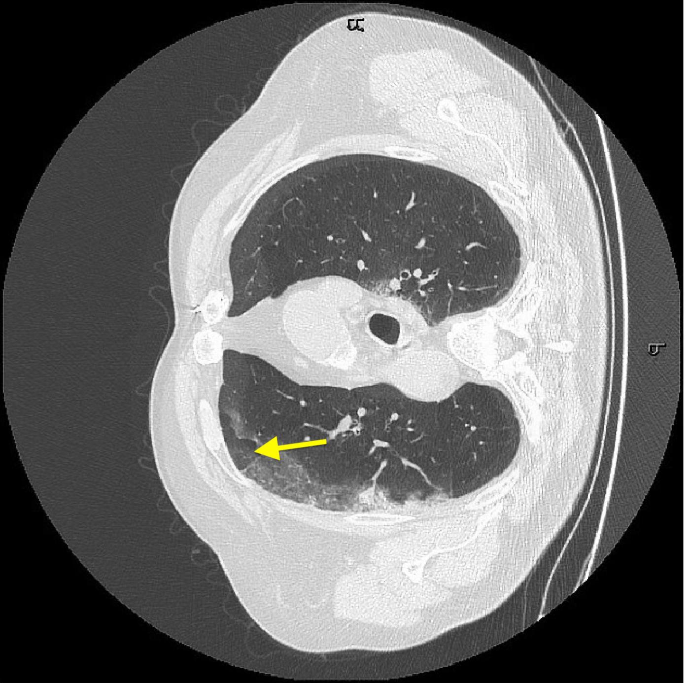
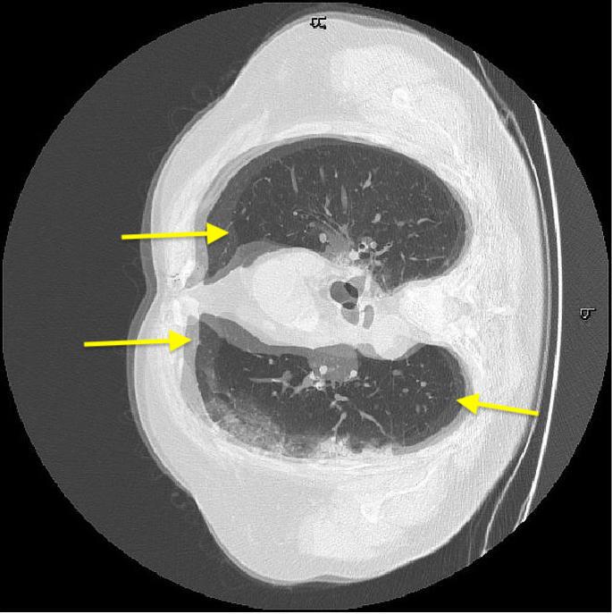
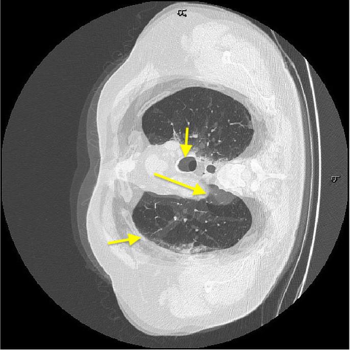
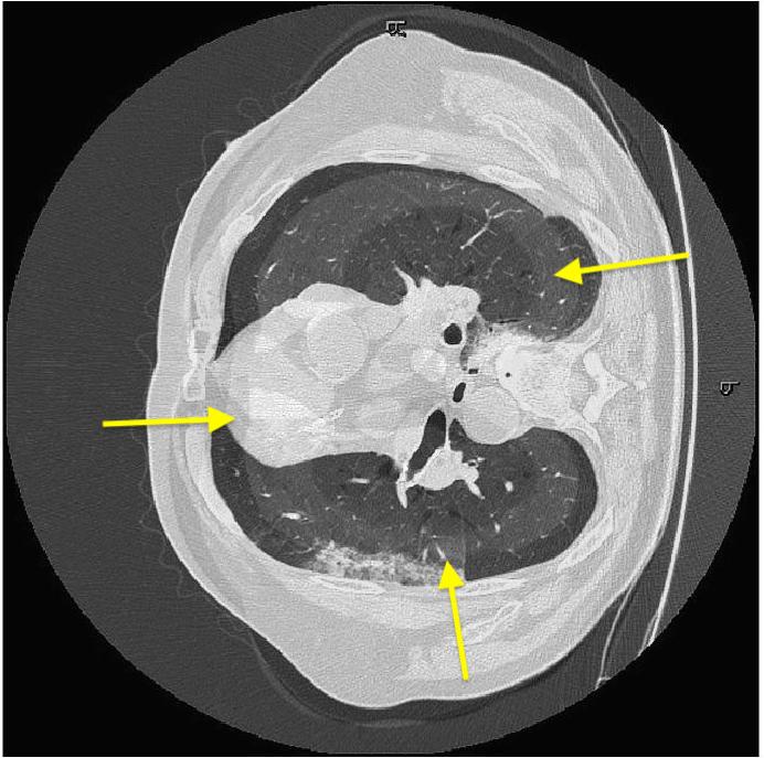
Although X-rays can be quickly acquired, CT screening provides a richer 3D view of the lung better suited for diagnosis. Recent studies of [28, 163, 54, 53, 56, 52, 122, 120, 118] provide evidence that CT scans (Figure 1) can be used to identify COVID-19 biomarkers such as ground-glass opacity (GGO) in the early stage, and pulmonary consolidation in the late stage. Thus qualitative evaluation of infection and longitudinal changes in CT scans can provide useful and important information for detecting COVID-19.

Recent methods such as [148, 132, 70, 40, 15, 160, 92, 75, 95, 142, 154, 72, 9] have proposed deep learning (DL) systems to detect COVID-19 patients from CT/Xray. Wang et al. proposed COVID-Net to identify COVID-19 cases from chest xrays [157, 143, 65, 144, 74, 136, 134, 153, 146]. [165, 105, 145, 104, 171, 81, 80, 79, 101] proposed an anomaly detection model to assist radiologists in analyzing a large databse of chest X-ray images. [162, 127, 43, 99, 141, 98, 109, 140, 55] developed a location-attention oriented model to calculate the infection probability of COVID-19 from CT images while a weakly-supervised DL method was developed in [169, 76, 126, 124, 125, 123, 49, 51, 155] for 3D CT volumes.

In comparison to classification (or diagnosis) related works, segmentation of pathological regions (e.g., infection areas) has received less attention [[16, 147, 50, 47, 121, 115, 116, 117, 119, 112]]. Segmentation of infected regions from CT is challenging due to: 1) high variation in texture, size and position of infections in CT scans. For example, consolidations are small leading to many false-negatives. 2) Low inter-class variance. GGO boundaries often have low contrast and blurred appearances making their identification a challenge for algorithms. 3) Difficulties in collecting a large labeled database within a a short time frame for DL systems.

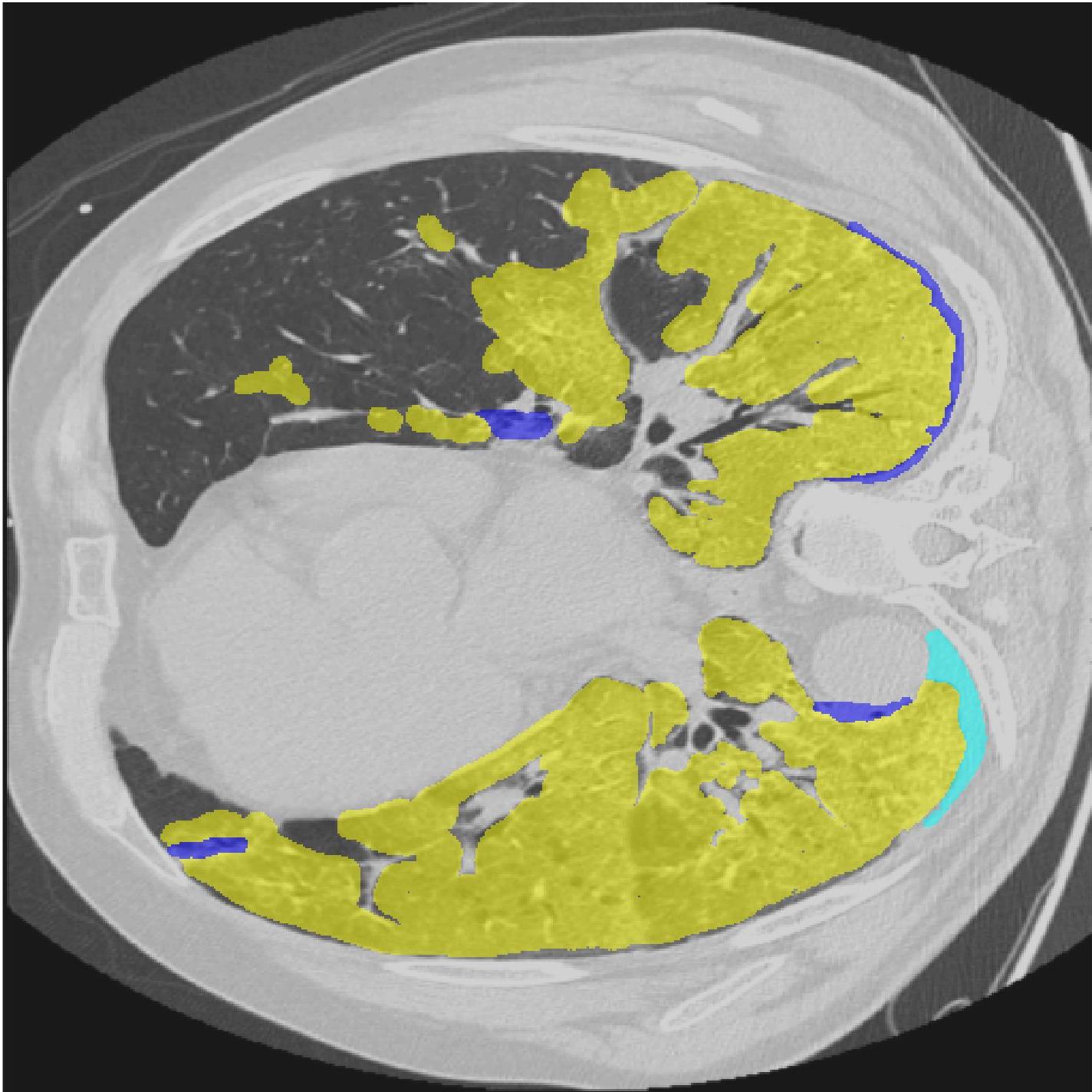
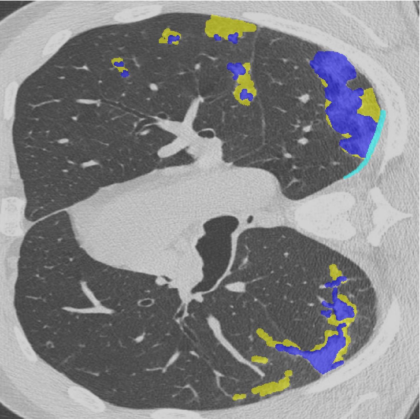
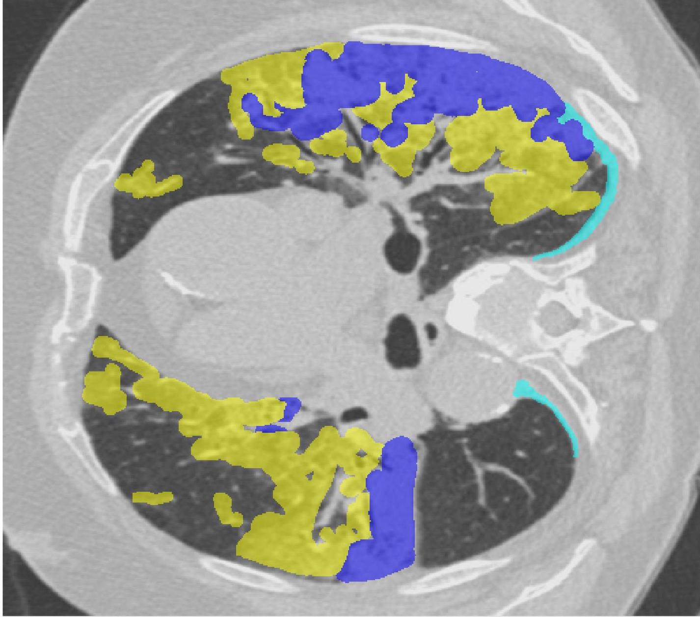
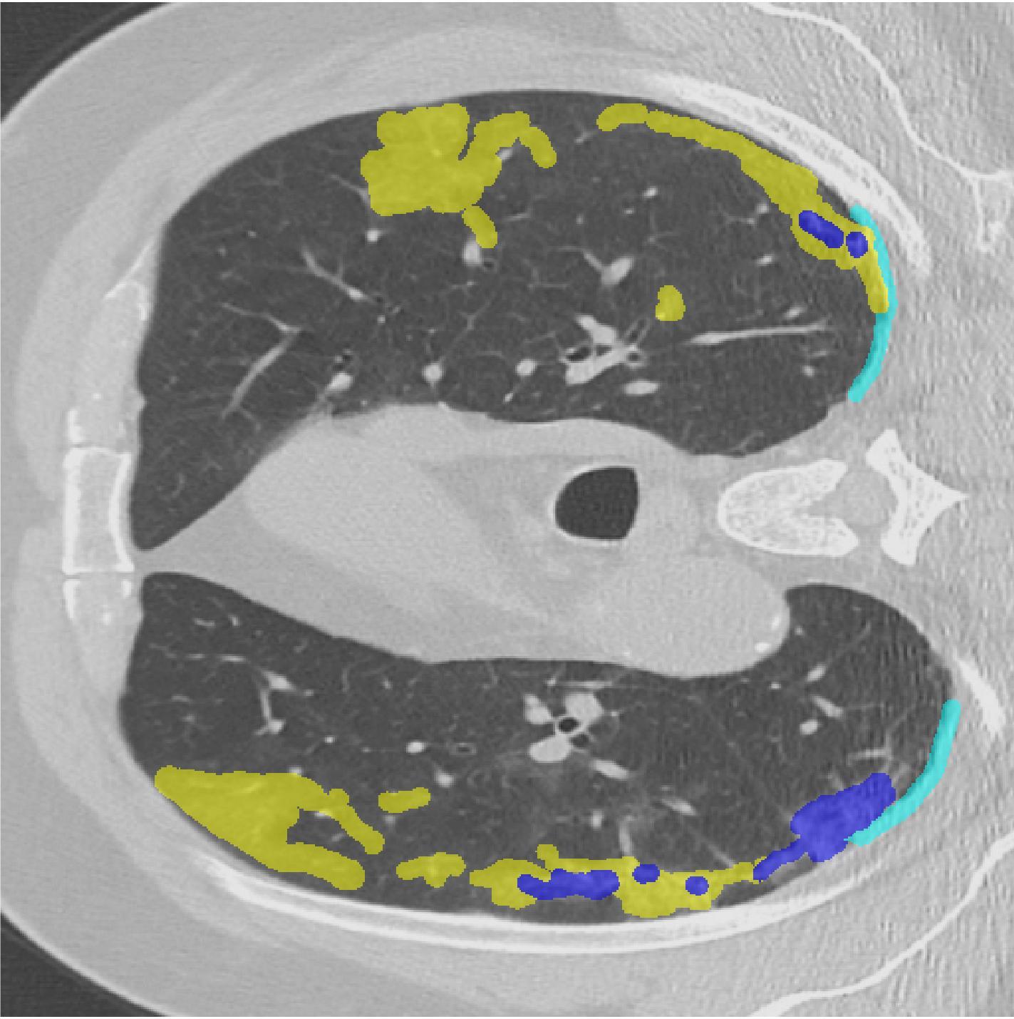
Furthermore, acquiring high quality pixel-level annotation of lung infections in CT scans is expensive and time-consuming. Manual delineation of lung infections is tedious and time-consuming, and infection annotations is a highly subjective task. Large scale dataset annotations for segmentation require pixel labels, which is time consuming and involves high degree of clinical expertise. The problem is particularly acute for pathological images (as in the case of COVID infections) since it is difficult to obtain diverse images for less prevalent disease conditions, necessitating data augmentation. We propose a generative adversarial network (GAN) based approach for pathological image augmentation and demonstrate its efficacy in COVID pathological region segmentation. Figure 2 shows example cases of synthetic images generated by our method and other competing techniques.

(a)	(b)	(c)	(d)	(e)

Figure 1: Example of images showing disease pathologies such as ground glass opacity, consolidation and pleural effusion.

(a)	(b)	(c)	(d)	(e)

Figure 2: (a) Base image with lung and infection regions highlighted; Example of generated images using: (b) Our proposed $GeoGAN$ method; (c) [166]; (d) $DAGAN$ method by [1]; (e) $cGAN$ method by [71]. Artifact regions are indicated by yellow arrows.

Traditional augmentations such as image rotations or deformations have limited benefit as they do not fully represent the underlying data distribution of the training set and are sensitive to parameter choices. Recent data augmentation methods of [25, 131, 11, 113, 108, 106, 114, 129, 103, 69, 139, 39, 32, 33, 13, 73, 62, 63] use generative adversarial network (GAN), [[23]], and show moderate success for medical image classification. However, they have limited relevance for segmentation since they do not model geometric relation between different organs and most augmentation approaches do not differentiate between normal and diseased samples. Hence there is a need for augmentation methods that consider the geometric relation between different anatomical regions and generate distinct images for diseased and normal cases.

II Related Work

II-A Chest CT Segmentation

Segmentation of lungs from chest CT scans is a widely explored topic [150, 12, 61, 91, 67, 42, 22] since it facilitates diagnosis and quantification of lung diseases [24]. [36, 110, 66, 59, 64, 5, 83, 84, 48] use support vector machines (SVM) to detect lung nodules from CT scans.Nodule extraction is challenging due to similar appearance with the background. Deep learning algorithms have been able to overcome this challenge by learning powerful discriminative features. [159, 88, 4, 87, 3, 89, 90] use CNNs to segment lung nodules from heterogeneous CT scans. [31, 86, 85, 107, 94, 20, 2, 111, 26, 135] make use of GAN-synthesized data to improve the performance of a discriminative model for pathological lung segmentation. [30] employ two deep networks to segment lung tumors from CT scans by adding multiple residual streams of varying resolutions.

II-B Deep Learning For Imaging Based COVID-19 Analysis

[158] use a modified inception network of [152] for classifying COVID-19 patients and normal controls. Instead of directly training on complete CT images, they trained the network on the regions of interest, which are identified by two radiologists based on the features of pneumonia. [17] use CT images to train a U-Net++ [170] for identifying COVID-19 patients that performs comparably with expert radiologists. DL approaches have also been used for segmenting infection regions in lung CT [19] and for lung infection quantification [132, 16, 147] of COVID-19.

II-C Data Augmentation (DA)

While conventional augmentation approaches (such as rotation, scaling, etc) can generate a large database, they do not add much data diversity. They are also sensitive to parameter values [18], variation in image resolution, appearance and quality [45]. Recent DL based methods trained with synthetic images outperform those trained with standard DA over classification and segmentation tasks. [1] proposed DAGAN for image generation in few shot learning systems. [166] proposed a learning-based registration method to register images to an atlas, use corresponding deformation field to deform a segmentation mask and obtain new data. [71] used conditional GAN (cGAN) for generating informative synthetic chest Xray images conditioned on a perturbed input mask.

GANs have also been used for generating synthetic retinal images in [167] and brain magnetic resonance images (MRI) in [25, 149], image registration [93] and generating higher strength MRI from their low strength acquisition counterparts [164]. Generated images have implicit variations in intensity distribution but there is no explicit attempt to model attributes such as shape variations that are important to capture different conditions across a population. [130] augmented medical images with simulated anatomical variations but demonstrate inconsistent performance based on transformation functions and parameter settings.

II-D Image Generation Using Uncertainty

[35] used approximate Bayesian inference for parameter uncertainty estimation in scene understanding, but did not capture complex correlations between different labels. [44] proposed a method to generate different samples using an ensemble of $M$ networks while [138] present a single network with $M$ heads for image generation. [151] proposed a method based on conditional variational autoencoders (cVAE) to model segmentation masks, which improves the quality of generated images. In probabilistic UNet [38], cVAE is combined with UNet [133] to generate multiple segmentation masks, although with limited diversity since randomness is introduced at highest resolution only. [6] introduced a framework to generate images with a greater diversity by injecting randomness at multiple levels.

II-E Our Contribution

Since annotating medical images is a time consuming task, it is challenging to obtain manually annotated segmentation masks to model the geometrical relation between different labels in the image. To overcome this challenge we propose to use a weakly supervised segmentation approach to generate labeled segmentation maps. The generated segmentation maps are then used to model the geometric relationship between the different pathological regions.

Based on the premise that improved data augmentation yields better segmentation performance in a DL system, we hypothesize that improved generation of synthetic images is possible by considering the intrinsic relationships between shape and geometry of anatomical structures [7]. In this paper we present a Geometry-Aware Shape Generative Adversarial Network (GeoGAN) that learns to generate plausible images of the desired anatomy (e.g.,COVID infected areas in the lung) while preserving learned relationships between geometry and shape. We make the following contributions:

1. Incorporating geometry information contributes to generation of realistic and qualitatively different medical images and shapes compared to standard DA. Other works such as [71, 167] do not incorporate this geometric relationship between anatomical parts.

2. Use of uncertainty sampling and conditional shape generation on class labels to introduce diversity in the mask generation process. Compared to previous methods we introduce diversity at different stages (different from [71, 167, 38]) and introduce an auxiliary classifier (different from [6, 151] ) for improving the quality and accuracy of generated images.

III Method

Our augmentation method: 1) models geometric relationship between multiple segmentation labels; 2) preserves disease class label of original image to learn disease specific appearance and shape characteristics; and 3) introduces diversity in the image generation process through uncertainty sampling. We demonstrate our method’s capability by training it on a dataset of CT lung images having annotations of COVID infected areas. However, in real world scenarios it is difficult to find datasets with such detailed annotations, especially in the case of COVID-19. Hence we introduce a weakly supervised segmentation (WSS) step that segments a CT image into different labeled regions using only the image labels of prevalent pathologies. The resulting label map enables us to learn the geometric relationship between different labels, which is essential to synthesize realistic images for data augmentation.

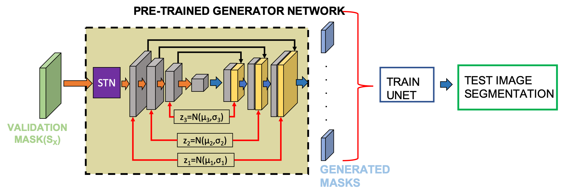
Figure 3 shows the training workflow using a modified UNet based generator network. The set of images and their WSS-obtained segmentation masks are used to train the generator while the discriminator provides feedback to improve the generator output. Figure 4 depicts generation of synthetic images after training is complete and their subsequent use in training a UNet for image segmentation at test time.

Figure 3: Overview of the steps in the training stage of our method. The images ($X$) and corresponding segmentation masks ($S_{X}$) are input to a STN whose output is fed to the generator network. Generator network is based on UNet architecture, and diversity through uncertainty sampling is injected at different levels. The generated mask $S_{X}^{{}^{\prime}}$ is fed to the discriminator which evaluates its accuracy based on $L_{class}$, $L_{shape}$ and $L_{adv}$. The provided feedback is used for weight updates to obtain the final model.

Figure 4: Depiction of mask generation. The trained generator network is used on validation set base images and masks to generate new images that are used to train a segmentation network (UNet or Dense UNet). The model then segments infected regions from test images.

III-A Weakly Supervised Segmentation

In order to obtain pixel labels from the image labels in a weakly supervised setting we solve a instance-level classification problem where pixels are instances. Subsequently, existing well-developed fully supervised segmentation methods can be applied. We use a combined Multiple Instance Learning (cMIL) for instance classification [161]. The image is split into $N\times N$ grids (instances) of equal size where instances from the same image are in the same bag. In cMIL, two MIL-based classifiers with different instance selection criteria ($Max-Max$ and $Max-Min$) are used to select instances to construct the instance-level dataset for subsequent classification.

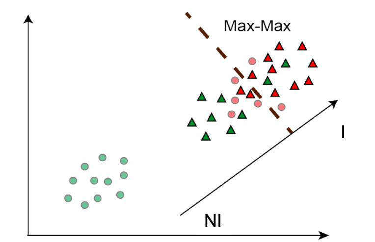
The selected instance can be considered as the representative of its corresponding image, which determines the image class.If the image is labeled ‘infected’ ($I$) we reason that at least one instance is infected. On the other hand, if the label of the image is ‘not infected’ ($NI$), all the instances in it are $NI$. For both $I$ and $NI$ images, $Max-Max$ selects the instance with maximum $I$ response. As shown in Figures 5 (a) and (b), during the training stage the $Max-Max$ criterion will select the instance with maximum $I$ response as the $NI$ example from the $NI$ samples. Therefore, the model trained with these data would give a decision boundary biased towards $I$ leading to misclassification of $I$ instances with lower responses (as shown by light red circles). For example, $I$ instances with similar appearances to $NI$ may get misclassified.

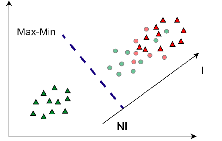
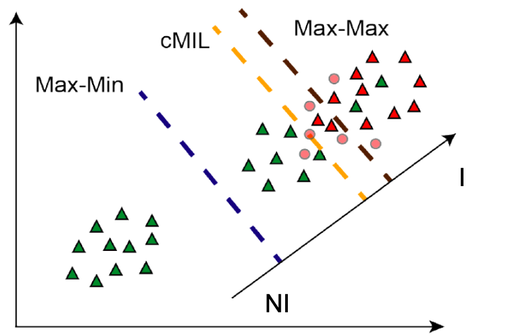
$Max-Min$ acts as a countermeasure that selects the instances with the highest $I$ response for $I$ images and the instances with the lowest response for $NI$ images. As shown in Figure 5(c), $Max-Min$ tends to have an opposite effect compared to $Max-Max$. Therefore, in cMIL we combine these two criteria to obtain a balanced instance-level dataset to be used in fully supervised learning (see Figure5 (d)). It is worth noting that, for $NI$ images, although each instance is $NI$, we only use the selected instances to avoid data imbalance.

Using a ResNet-50 architecture we train the two MIL-based classifiers separately under the same configuration: in the forward pass, we use the $Max-Max$ (or $Max-Min$ for the other classifier) criterion to select one instance from each bag based on their predictions, and the prediction of the selected instance is regarded as the prediction of the image. In the backpropagation step, we use the cross entropy loss between the image-level label and the prediction of the selected instance to update the classifier’s parameters. The loss function for each classifier is defined as follows:

$$Loss=-\sum_{j}\left(y_{j}\log\hat{p}_{j}+(1-y_{j})\log(1-\hat{p}_{j})\right),$$ (1)

where $\hat{p}_{j}=S_{criterion}(\{f(b_{i})\})$, $b_{i}$ are the instances in image $j$, $f$ is the classifier, $S_{criterion}\in\{Max-Max,Max-Min\}$. $S_{criterion}$ selects the target instance using the defined criterion, $y_{j}$ is the image-level label.

For Max-Max criterion:

$$S_{Max-Max}(\{f(b_{i})\})=\max_{i}{f(b_{i})}$$ (2)

For Max-Min criterion:

$$S_{Max-Min}({f(b_{i})})=\begin{cases}\max_{i}{f(b_{i})}&\text{if}~{}y=1\\ \min_{i}{f(b_{i})}&\text{if}~{}y=0\end{cases}$$ (3)

After training, we feed the same training data into the two trained classifiers and select the instances under the corresponding criterion, then the predictions are considered as their labels. We combine the instances selected by the two trained classifiers to construct the final fully supervised instance-level dataset. Note that we discard those potentially confusing samples whose predicted labels are different from their corresponding image-level labels.

Retrain and Relabel

Once the instance-level dataset is selected, we train an instance classifier in a fully supervised manner. Similar to cMIL we use a ResNet-50 and name this step as retrain. Then, we split the original image into latticed instances and relabel them using the trained instance-level classification model. For each image, we obtain $N^{2}$ high-quality instance labels from a single image-level label.

III-A1 Segmentation

With enriched supervision information, the instance level labels are directly assigned to the corresponding pixels, producing approximate pixel-level labels. Therefore, we can train segmentation models in a fully supervised way using well-developed architectures such as UNet++ [170].

Training with Image-Level Constraints

In order to maximize the utility of the original image-level supervision information, in the retrain step, we can add the original image-level data as one additional input source going through the classifier. The image-level constraint is imposed under Max-Max and Max-Min criteria to the instance level, the total loss is defined as the sum of the retrain loss and the constraint loss:

$$Loss=w_{1}\times Loss_{constrain}+w_{2}\times Loss_{retrain}$$ (4)

where $w_{1}$ and $w_{2}$ are the weights of the two losses. We set $w_{1}=w_{2}$ in our experiments.

$$Loss_{constrain}=-\sum_{S_{criterion}}(y\log\hat{p}+(1-y)\log(1-\hat{p})),$$ (5)

where $\hat{p}=S_{criterion}({f(b_{i})})$, $b_{i}$ represents the selected instance, $f$ is the image-level constrain route, $S_{criterion}\in\{Max-Max,Max-Min\}$, and $y$ is the image-level label.

$$Loss_{retrain}=-\sum_{j}(y_{j}\log\hat{y}_{j}+(1-y_{j})log(1-\hat{y}_{j}))$$ (6)

where $\hat{y}_{j}=g(n_{j})$, $n_{j}$ represents the input instance, $g$ is the retrain route, and $y_{j}$ is the instance-level label.

(a)	(b)
(c)	(d)

Figure 5: Intuition behind two instance selection criteria named $Max-Max$ and $Max-Min$. Red and green circles represent the $I$ and $NI$ instances, respectively. We use triangles to represent the selected instances, and circles with light colors to represent the instances that are not selected. Each dotted line represents the decision boundary of the classifier, which is trained with the selected instances. Each ellipse represents an image (or a bag in MIL). cMIL, which combines $Max-Max$ and $Max-Min$, achieves a better decision boundary.

III-B Geometry Aware Shape Generation

Let us denote an input image as $x$, the corresponding segmentation masks as $s_{x}$ and the disease class label of $x$ as $l_{x}$. Our method learns to generate a new image and segmentation label map from a base image and its corresponding mask. The first stage is a spatial transformer network (STN) [29] that transforms the base mask to a new shape with different attributes of location, scale and orientation. The transformations used to obtain new segmentation mask $s_{x}^{{}^{\prime}}$ are applied to $x$ to get corresponding transformed image $x^{{}^{\prime}}$. Since the primary aim of our approach is to learn contours and other shape specific information of anatomical regions, a modified UNet architecture as the generator network effectively captures hierarchical information of shapes. It also makes it easier to introduce diversity at different levels of image abstraction.

The generator $\textbf{G}_{g}$ takes input $\textbf{s}_{x}$ and a desired label vector of output mask $c_{g}$ to output an affine transformation matrix A via a STN, i.e., $\textbf{G}_{g}$($\textbf{s}_{x},c_{g})=\textbf{A}$. A is used to generate $s_{x}^{{}^{\prime}}$ and $x^{{}^{\prime}}$. The discriminator $\textbf{D}_{class}$ determines whether output image preserves the desired label $c_{g}$ or not. The discriminator $\textbf{D}_{g}$ is tasked with ensuring that the generated masks and images are realistic. Let the minimax criteria between $\textbf{G}_{g}$ and $\textbf{D}_{g}$ be $\min_{\textbf{G}_{g}}\max_{\textbf{D}_{g}}\textbf{L}_{g}(\textbf{G}_{g},\textbf{D}_{g})$. The loss function $\textbf{L}_{g}$ has three components

$$L_{g}=L_{adv}+\lambda_{1}{L}_{class}+\lambda_{2}{L}_{shape}$$ (7)

where 1) $\textbf{L}_{adv}$ is an adversarial loss to ensure $\textbf{G}_{g}$ outputs realistic deformations; 2) $\textbf{L}_{class}$ ensures generated image has characteristics of the target output class label (disease or normal); and 3) $\textbf{L}_{shape}$ ensures new masks have realistic shapes. $\lambda_{1},\lambda_{2}$ balance each term’s contribution.

Adversarial loss

- $\textbf{L}_{adv}(\textbf{G}_{g},\textbf{D}_{g})$: The STN outputs $\widetilde{A}$, a prediction for A conditioned on $\textbf{s}_{x}$ and a new semantic map $\textbf{s}_{x}\oplus\widetilde{A}(\textbf{s}_{x})$ is generated. $\textbf{L}_{adv}$ is defined as:

$$\begin{split}L_{adv}(G_{g},D_{g})=\mathbb{E}_{x}\left[\log D_{g}(\textbf{s}_{x}\oplus\widetilde{A}(\textbf{s}_{x}))\right]\\ +\mathbb{E}_{\textbf{s}_{x}}\left[\log(1-D_{g}(\textbf{s}_{x}\oplus\widetilde{A}(\textbf{s}_{x})))\right],\end{split}$$ (8)

Classification Loss

- $\textbf{L}_{class}$: The affine transformation A is applied to the base image x to obtain the generated image $\textbf{x}^{{}^{\prime}}$. We add an auxiliary classifier when optimizing both $\textbf{G}_{g}$ and $\textbf{D}_{g}$ and define the classification loss as,

$$L_{class}=\mathbb{E}_{\textbf{x}^{{}^{\prime}},c_{g}}[-\log D_{class}(c_{g}|x^{\prime})],$$ (9)

where the term $D_{class}(c_{g}|x^{\prime})$ represents a probability distribution over classification labels computed by $D$.

Shape Loss

-$\textbf{L}_{shape}$: We intend to preserve the relative geometric arrangement between the different labels. The generated mask has regions with different assigned segmentation labels because the base mask (from which the image was generated) already has labeled layers. Let us denote by $s_{i}$ the image region (or pixels) in $\textbf{s}_{x}$ assigned label $i$. Consider another set of pixels, $s_{j}$, assigned label $j$. We calculate $P_{shape}(l_{i}|s_{j},s_{i})$, which is, given regions $s_{i},s_{j}$, the pairwise probability of $s_{i}$ being label $i$. If $n$ denotes the total number of labels, for every label $i$ we calculate the $n-1$ such probability values and repeat it for all $n$ labels. Thus

$$L_{shape}=\frac{1}{n\times(n-1)}\sum_{i,j}^{i\neq j}P_{shape};~{}(i,j)\in\{1,\cdots,n\}$$ (10)

The probability value is determined from a pre-trained modified VGG16 architecture to compute $L_{shape}$ where the input has two separate maps corresponding to the label pair. Each map’s foreground has only the region of the corresponding label and other labels considered background. The conditional probability between the pair of label maps enables the classifier to implicitly capture geometrical relationships and volume information between the label pair without the need to define explicit features. The geometric relation between different labels will vary for infected and non-infected cases, which is effectively captured by our approach. To get the pre-trained VGG16 network we used a separate dataset of $24$ images with its WSS generated segmentation maps.

III-C Sample Diversity From Uncertainty Sampling

The generated mask $s_{x}^{\prime}$ is obtained by fusing $L$ levels of the generator $G_{g}$ (as shown in Figure 3), each of which is associated with a latent variable $z_{l}$. We use probabilistic uncertainty sampling to model conditional distribution of segmentation masks and use separate latent variables at multi-resolutions to factor inherent uncertainties. The hierarchical approach introduces diversity at different stages and influences different features (e.g., low level features at the early layers and abstract features in the later layers). Denoting the generated mask as $s$ for simplicity, we obtain conditional distribution $p(s|x)$ for $L$ latent levels as:

$$\begin{split}p(s|x)=\int p(s|z_{1},\cdots,z_{L})p(z_{1}|z_{2},x)\cdots\\ p(z_{L-1}|z_{L},x)p(z_{L}|x)dz_{1}\cdots dz_{L}.\end{split}$$ (11)

Latent variable $z_{l}$ models diversity at resolution $2^{-l+1}$ of the original image (e.g. $z_{1}$ and $z_{3}$ denote the original and $1/4$ image resolution). A variational approximation $q(z|s,x)$ approximates the posterior distribution $p(z|s,x)$ where $z=\{z_{1},...,z_{L}\}$. $\log p(s|x)=L(s|x)+KL(q(z|s,x)||p(z|s,x))$, where $L$ is the evidence lower bound, and $KL(.,.)$ is the Kullback-Leibler divergence. The prior and posterior distributions are parameterized as normal distributions $\mathcal{N}(z|\mu,\sigma)$.

Figure 3 shows example implementation for $L=3$. We use $6$ resolution levels and $L=4$ latent levels. Figure 3 shows the latent variables $z_{l}$ forming skip connections in a UNet architecture such that information between the image and segmentation output goes through a sampling step. The latent variables are not mapped to a 1-D vector to preserve the structural relationship between them, and this substantially improves segmentation accuracy. $z_{l}$’s dimensionality is $r_{x}2^{-l+1}\times r_{y}2^{-l+1}$, where $r_{x}$ , $r_{y}$ are image dimensions.

IV Experimental Results

IV-A Dataset Description

We use the following three different segmentation datasets:

CT Segmentation Dataset 1 (CTSeg1): The dataset consists of 100 axial CT images from different COVID-19 patients. All the CT images were collected by the Italian Society of Medical and Interventional Radiology. A radiologist segmented the CT images with $3$ labels: ground-glass (mask value =1), consolidation (=2) and pleural effusion (=3).

CT Segmentation Dataset 2 (CTSeg2): The second dataset is collected from $9$ axial volumetric CTs. It includes whole volumes and both positive and negative slices ($373$ out of the total of $829$ slices have been evaluated by a radiologist as positive and segmented).

CT Segmentation Dataset 3 (CTSeg3): This dataset contains $20$ labeled COVID-19 CT scans. Left lung, right lung, and infections are labeled by two radiologists and verified by an experienced radiologist.

IV-B Experimental Setup, Baselines and Metrics

Our method has the following steps: 1) Use the default training, validation, and test folds of the dataset. 2) Use training images to train the image generator. 3) Generate shapes from the training set and train UNet++ segmentation network [170] on the generated images. 4) Use trained UNet++ to segment test images. 5) Repeat the above steps for different data augmentation methods. Our model is implemented in PyTorch, on a NVIDIA TITAN X GPU. We trained all models using Adam optimiser [37] with a learning rate of $10^{-3}$ and batch-size of $16$. Batch-normalisation was used. The values of parameters $\lambda_{1}$ and $\lambda_{2}$ in Eqn. 7 were set by a detailed grid search on a separate dataset of $14$ volumes that was not used for training or testing. They were varied between $[0,1]$ in steps of $0.05$ by fixing $\lambda_{1}$ and varying $\lambda_{2}$ for the whole range. This was repeated for all values of $\lambda_{1}$. The best segmentation accuracy was obtained for $\lambda_{1}=0.92$ and $\lambda_{2}=0.9$, which were our final parameter values.

We denote our method as $GeoGAN_{WSS}$ (Geometry Aware GANs using the weakly supervised segmentation component), and compare it’s performance against other methods such as: 1) rotation, translation and scaling (denoted as DA-Data Augmentation); 2) $DAGAN$ - data augmentation GANs of [1]; 3) $cGAN$ - the conditional GAN based method of [71]; 4) $Zhao$- the atlas registration method of [166]; 5) $GeoGAN_{Manual}$ - Geometry Aware GANs using the manual segmentation maps for image synthesis. Segmentation performance is evaluated in terms of Dice Metric (DM), Hausdorff Distance (HD) and Mean Absolute error (MAE). DM of $1$ indicates perfect overlap and $0$ indicates no overlap, while lower values of MAE indicate better segmentation performance.

Algorithm Baselines.

The following variants of our method were used for ablation studies:

1. GeoGAN${}_{noL_{class}}$- GeoGAN_WSS without classification loss (Eqn.9).

2. GeoGAN${}_{noL_{shape}}$- GeoGAN_WSS without shape relationship modeling term (Eqn.10).

3. GeoGAN_NoSamp - GeoGAN_WSS without uncertainty sampling for injecting diversity to determine sampling’s relevance to the final network performance.

IV-C Efficacy of Weakly Supervised Semantic Segmentation

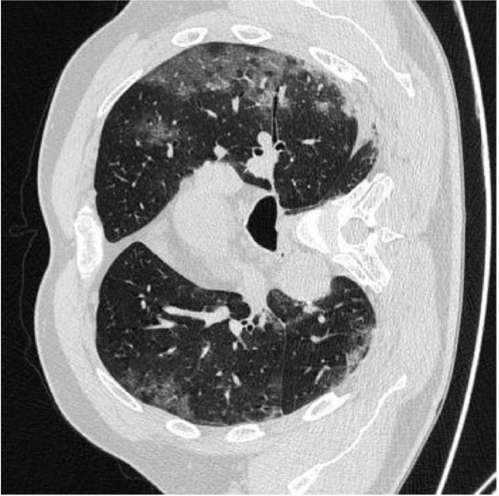
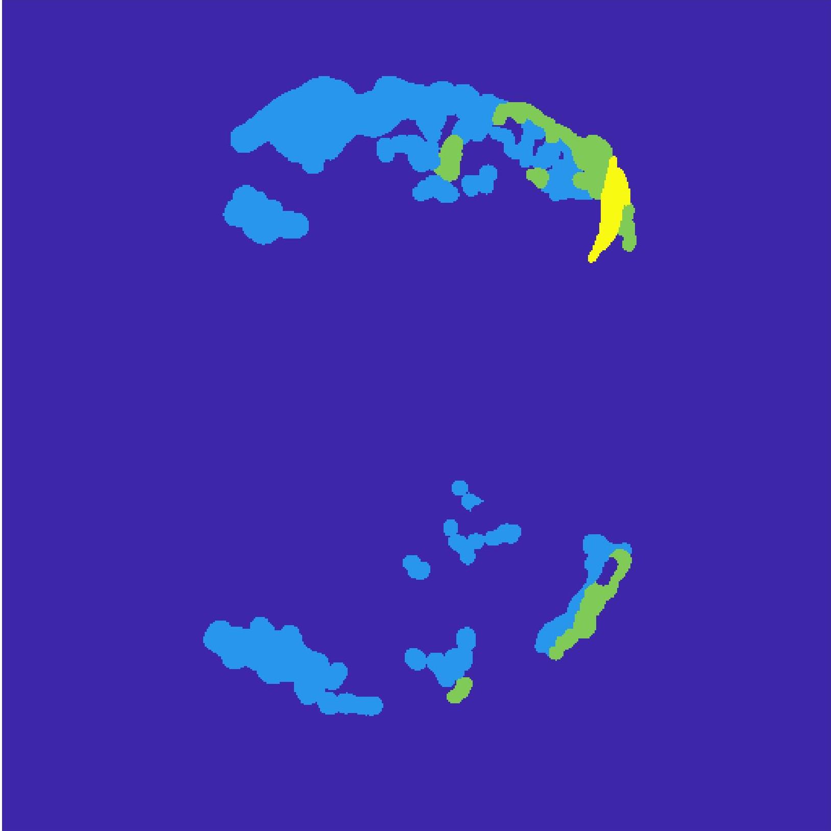
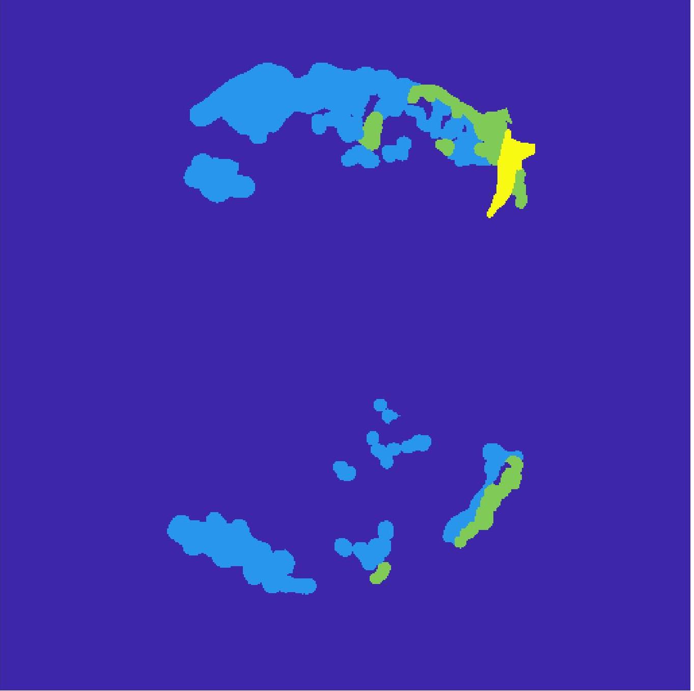
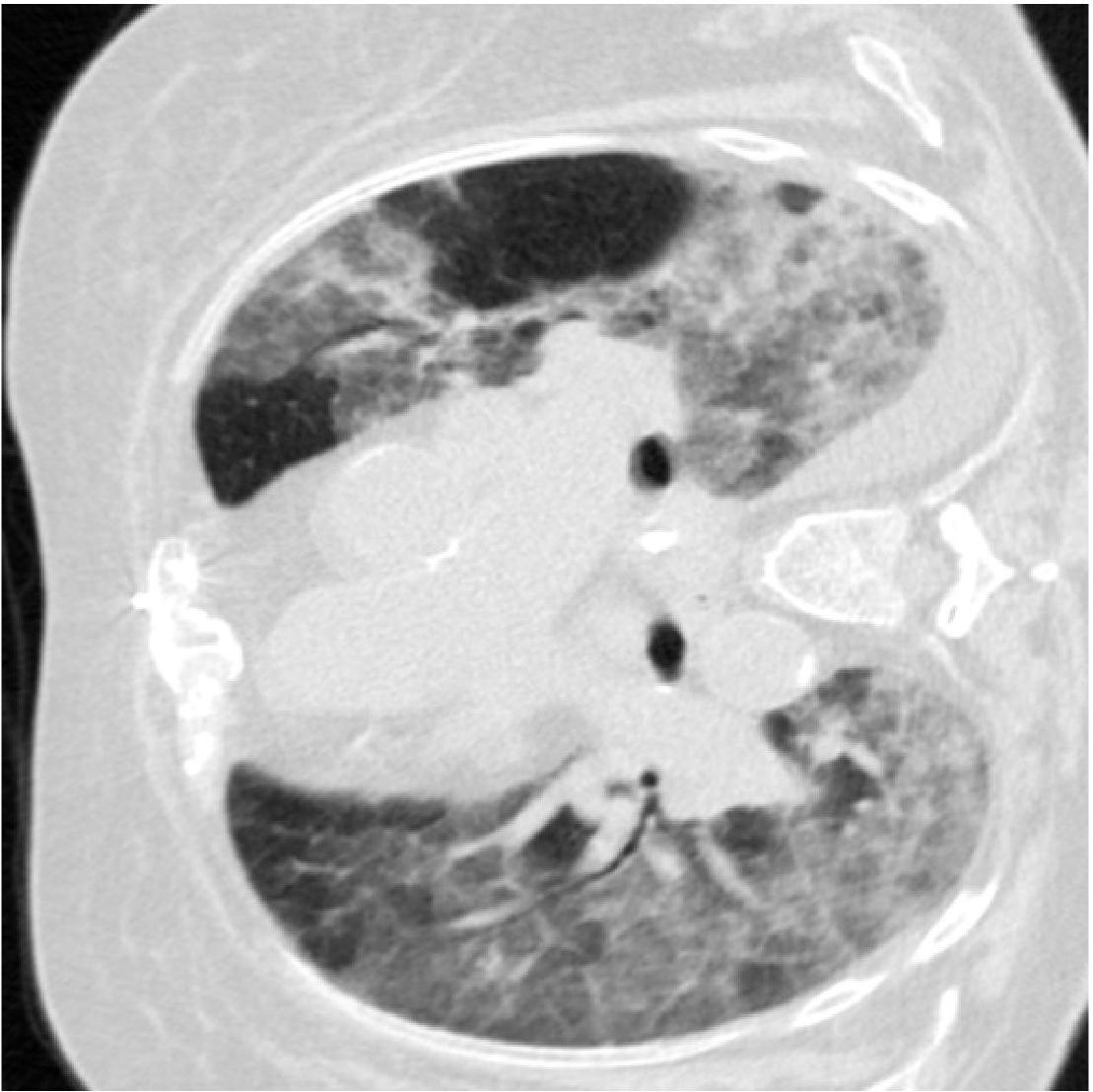
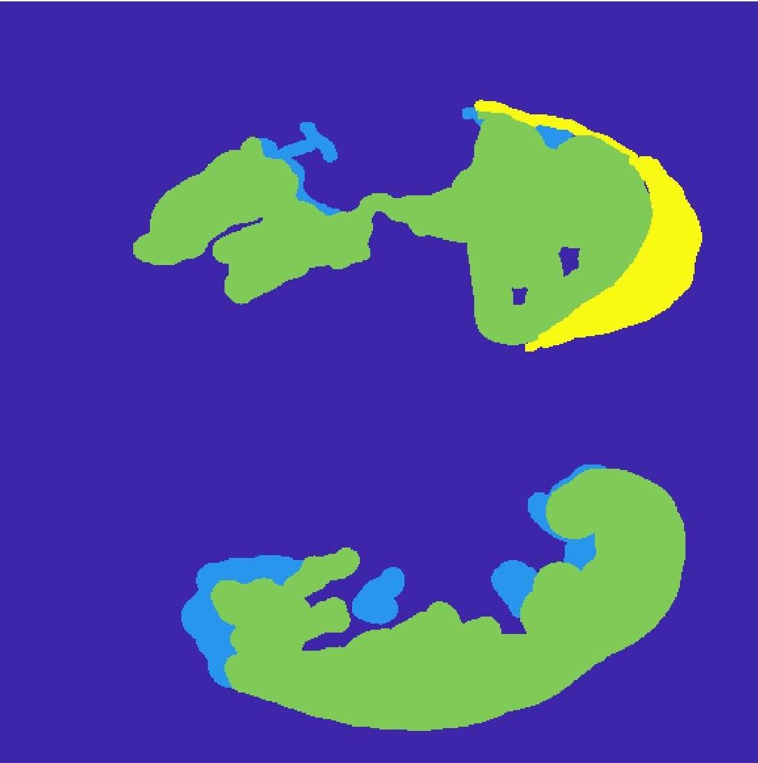
To quantify the accuracy of the weakly supervised segmentation step we compare the segmentation output with the manual segmentations and obtain $DM=0.926$, and $HD=6.5$ mm. These numbers indicate very good agreement with the expert’s manual annotations. Figure 6 shows two examples of an image, its ground truth label map, and the label map obtained from the weakly supervised segmentation step. We observe that the WSS map closely resembles the manual map with small regions of oversegmentation. Oversegmented label maps recover the entire annotated area and hence enable GeoGAN to learn the full range of geometrical relations between different labels. On the other hand, oversegmented maps also let the algorithm learn noisy features due to the fact that non-diseased regions are included as infections.

(a)	(b)	(c)

Figure 6: Results for weakly supervised segmentation compared to ground truth maps. (a) CT image; (b) manual ground truth segmentation label map; (c) label map generated by our weakly supervised approach. Light blue is label $1$ - ground glass opacity; Green is label $2$ - consolidation; Yellow is label $3$- pleural effusion.

IV-D Segmentation Results And Analysis

We hypothesize that a good image augmentation method should capture the different complex relationships between different labels, with the generated images leading to improvement in segmentation accuracy. Table I shows the average DM and MAE for different augmentation methods on the $CTSeg1$ dataset for infection regions. We also report the performance of the recent approach of [19] on the same dataset.

Table I shows the $p$ values comparing the results of all methods with $GeoGAN_{WSS}$ (except [19] since we do not have access to all segmentation masks). Results of $GeoGAN_{Manual}$ denote the best performance obtained with a given network since they are trained on clinician provide manual segmentation maps. $GeoGAN_{WSS}$’s results show that the WSS component is very accurate in obtaining semantic segmentation and can be used effectively where manual segmentation maps are unavailable.

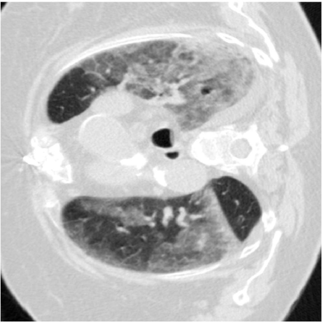
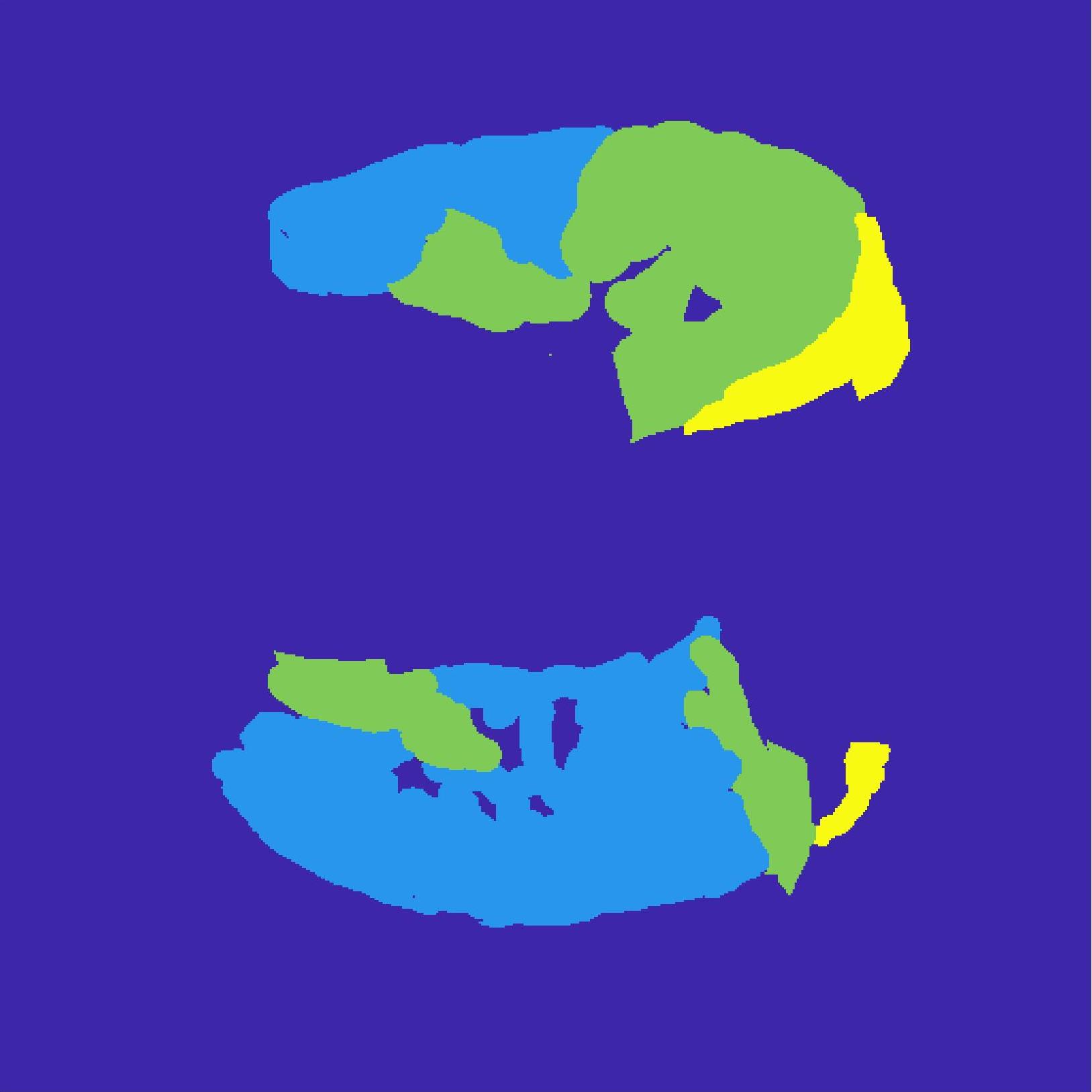
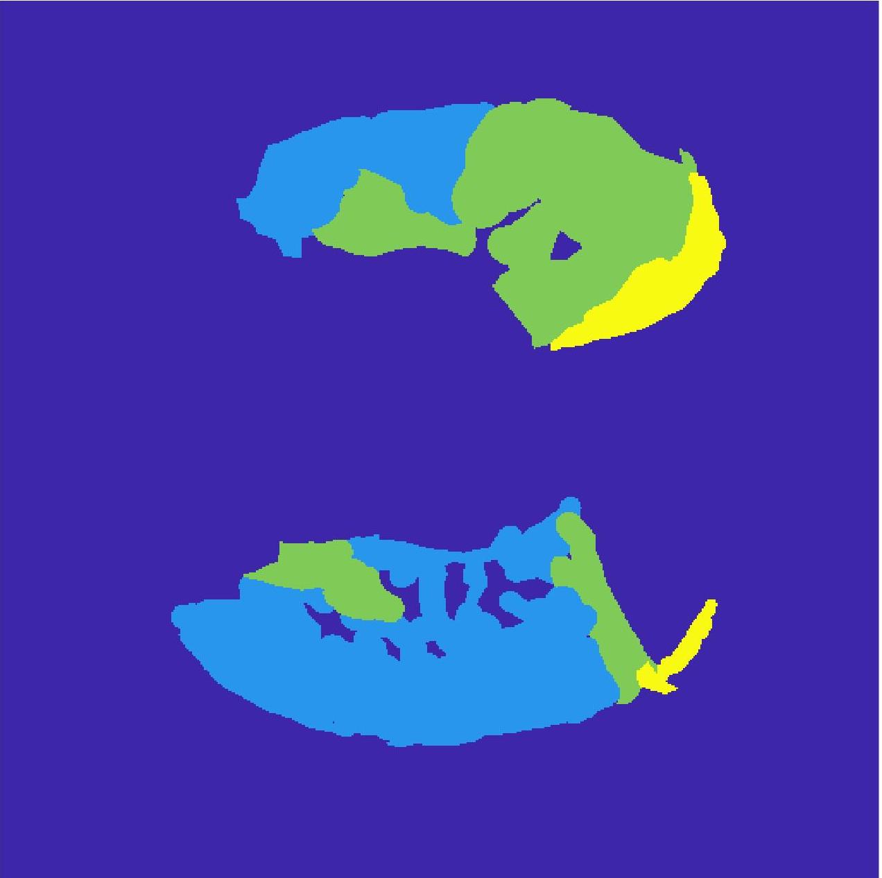
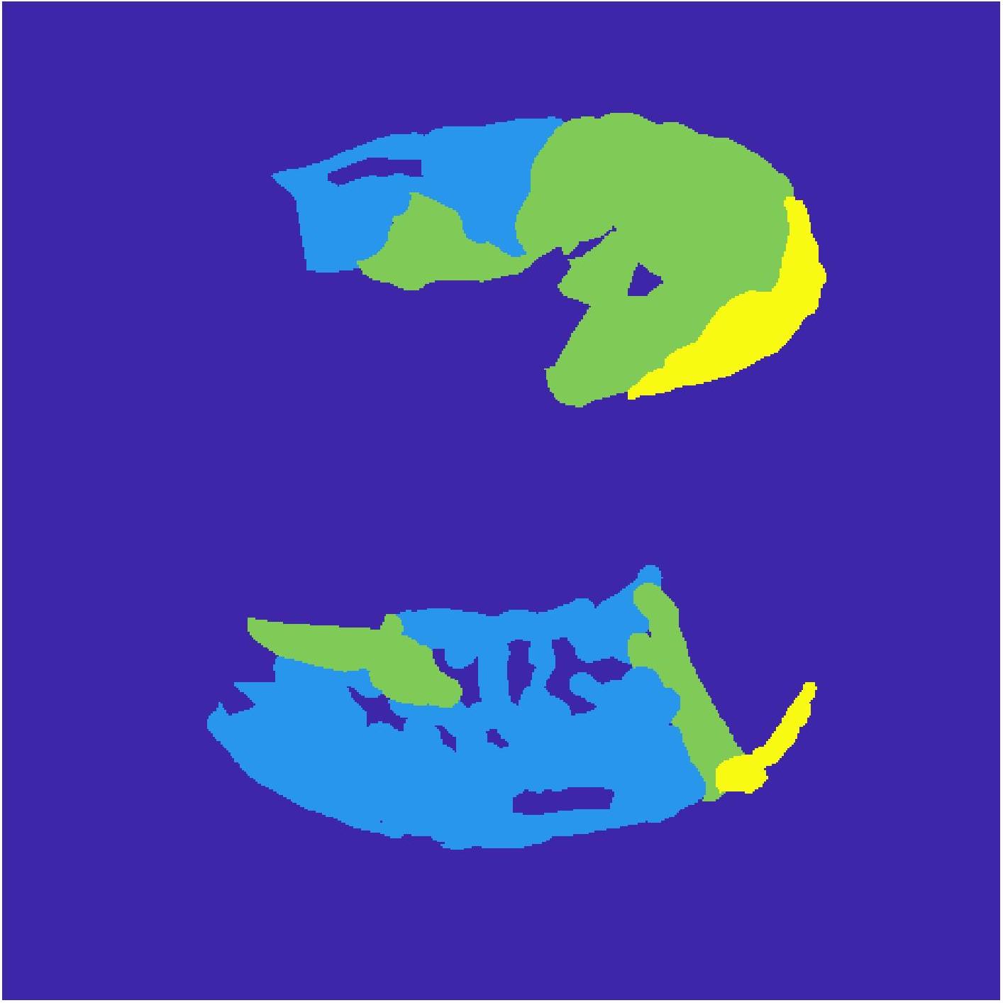
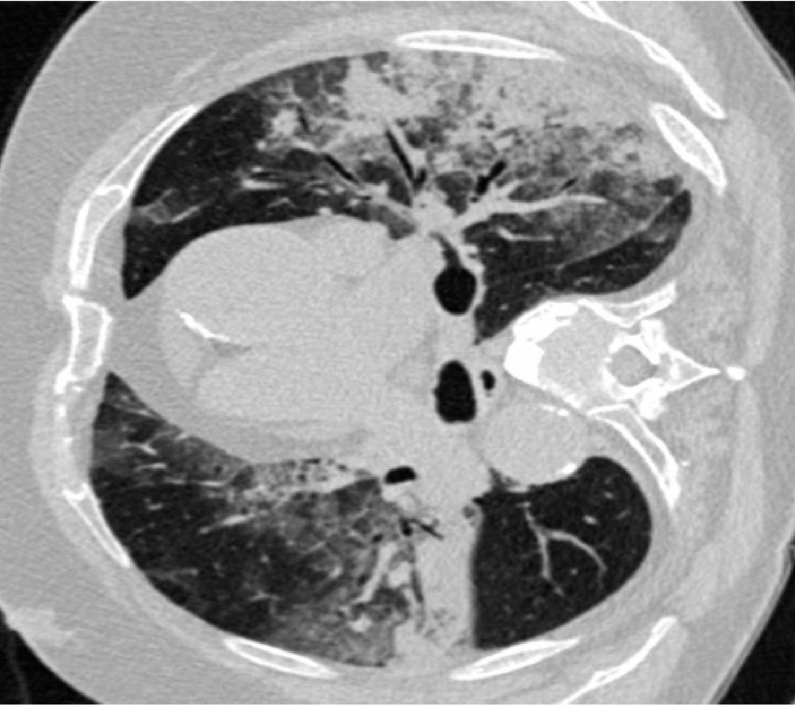
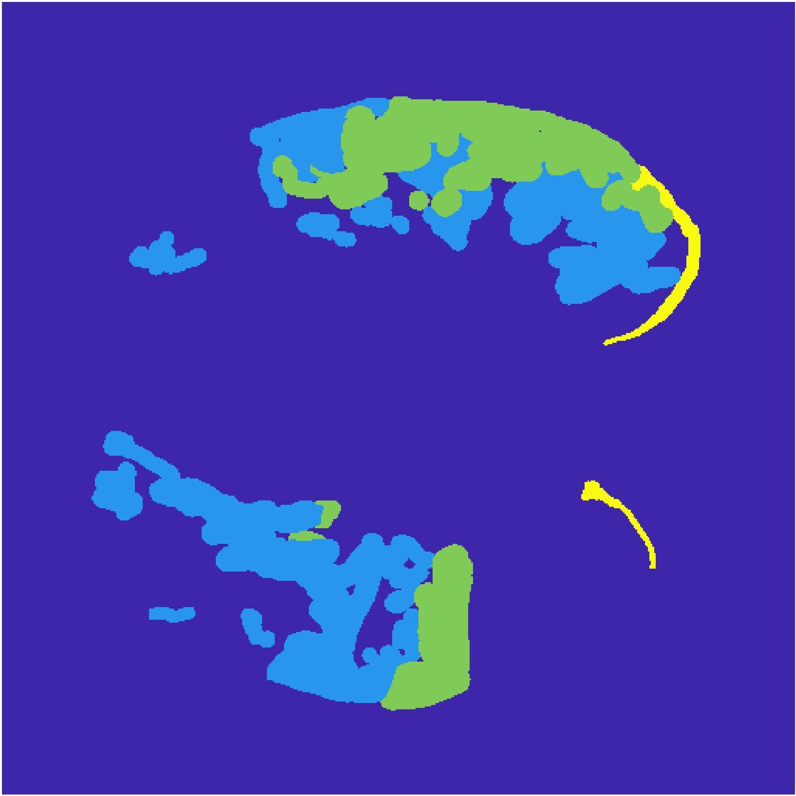
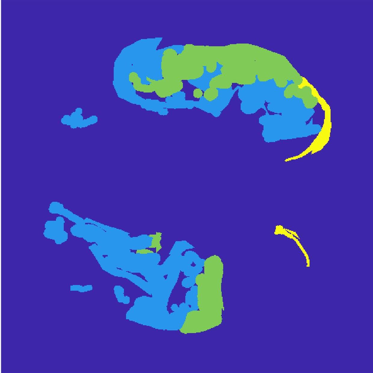
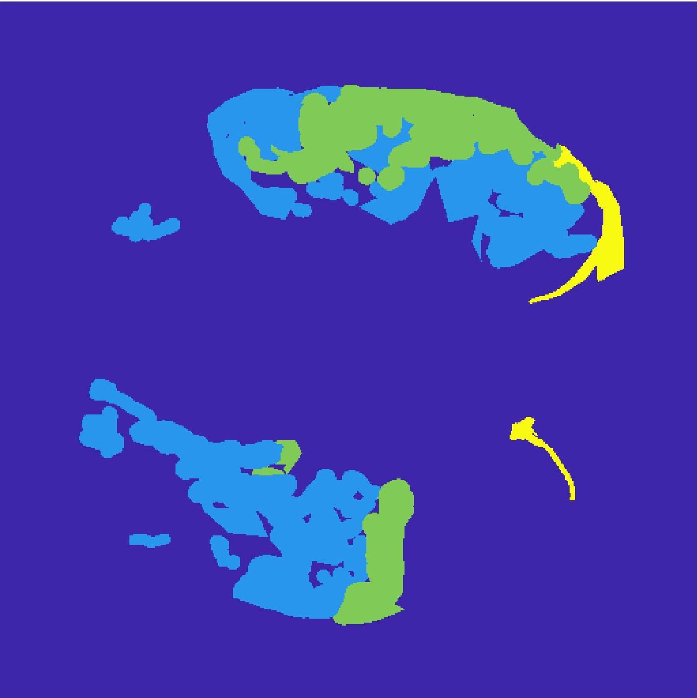
Figure 7 shows the segmentation results using a UNet++ trained on images from different methods. Figure 7 (a) shows the test image and Figure 7 (b) shows the manual mask. Figures 7 (c)-(f) show, respectively, the segmentation masks obtained by GeoGAN_WSS, [166], $DAGAN$ and $cGAN$.

Subsequently, in Tables II,III we show results of $GeoGAN_{WSS}$ (denoted as $GeoGAN$ for brevity) for datasets $CTSeg2$ and $CTSeg3$. Our method outperforms baseline conventional data augmentation and other competing methods by a significant margin. GeoGAN_WSS’s DM is higher than the DM value of the best performing method. We also perform better than [19] on $CTSeg1$, which uses semi-supervised approaches to outperform a UNet++ architecture (using conventional data augmentation). Our results clearly show that with better augmentation techniques we can do better than state of the art segmentation network architectures.

GeoGAN’s superior segmentation accuracy is attributed to it’s capacity to learn geometrical relationship between different labels (through $L_{shape}$) much better than competing methods. Thus our attempt to model the intrinsic geometrical relationships between different labels could generate superior quality masks.

	Comparison approaches				Proposed
	DA	DAGAN	cGAN	Zhao	GeoGANWSS	GeoGANManual	[19]
DM	0.704	0.719	0.738	0.752	0.781	0.789	0.764
	(0.17)	(0.12)	(0.09)	(0.08)	(0.05)	(0.03)	-
p	0.006	0.004	0.0005	0.0003	-	0.11	-
MAE	0.097	0.088	0.083	0.071	0.058	0.053	0.064
	(0.018)	(0.015)	(0.015)	(.017)	(.013)	(.012)	-
HD	13.9	12.7	10.9	9.1	8.3	8.2	-
	(4.1)	(3.9)	(3.8)	(3.1)	(2.4)	(2.3)	-

TABLE I: COVID Segmentation results for $CTSeg1$ dataset. Mean and standard deviation (in brackets) are shown. Best results per metric is shown in bold. $p$ values are with respect to $GeoGAN_{WSS}$

(a)	(b)	(c)	(d)	(e)	(f)

Figure 7: Segmentation results on the $CTSeg1$ dataset: (a) original test images; (b) manual segmentation masks. Masks generated using data generated by: (c) GeoGAN; (d) Zhao [166]; (e) $DAGAN$; (f) $cGAN$. The two rows correspond to two different images.

	Comparison approaches				Proposed
	DA	DAGAN	cGAN	Zhao	GeoGAN
DM	0.708	0.727	0.761	0.774	0.809
	(0.15)	(0.13)	(0.10)	(0.09)	(0.07)
HD	14.2	12.4	11.2	9.4	8.7
	(4.4)	(3.7)	(3.2)	(3.0)	(2.7)
MAE	0.112	0.094	0.088	0.079	0.073
	(0.011)	(0.009)	(0.010)	(0.008)	(0.006)
p	0.0007	0.005	0.0001	0.01	-

TABLE II: COVID Segmentation results for $CTSeg2$ dataset. Mean and standard deviation (in brackets) are shown. Best results per metric is shown in bold. $p-$values are with respect to GeoGAN.

	Comparison approaches				Proposed
	DA	DAGAN	cGAN	Zhao	GeoGAN
DM	0.723	0.762	0.779	0.793	0.815
	(0.12)	(0.10)	(0.13)	(0.08)	(0.05)
HD	13.7	12.4	11.2	9.0	7.8
	(4.2)	(3.6)	(3.9)	(3.3)	(3.1)
MAE	0.097	0.089	0.081	0.077	0.069
	(0.009)	(0.010)	(0.008)	(0.006)	(0.005)
p	0.008	0.003	0.009	0.01	-

TABLE III: COVID Segmentation results for $CTSeg3$ dataset. Mean and standard deviation (in brackets) are shown. Best results per metric is shown in bold.$p-$values are with respect to GeoGAN.

IV-E Ablation Studies.

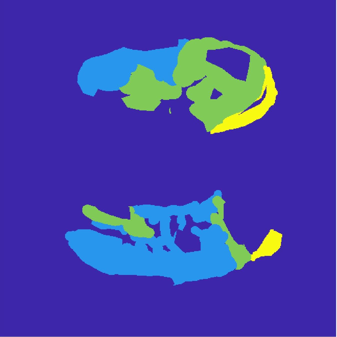
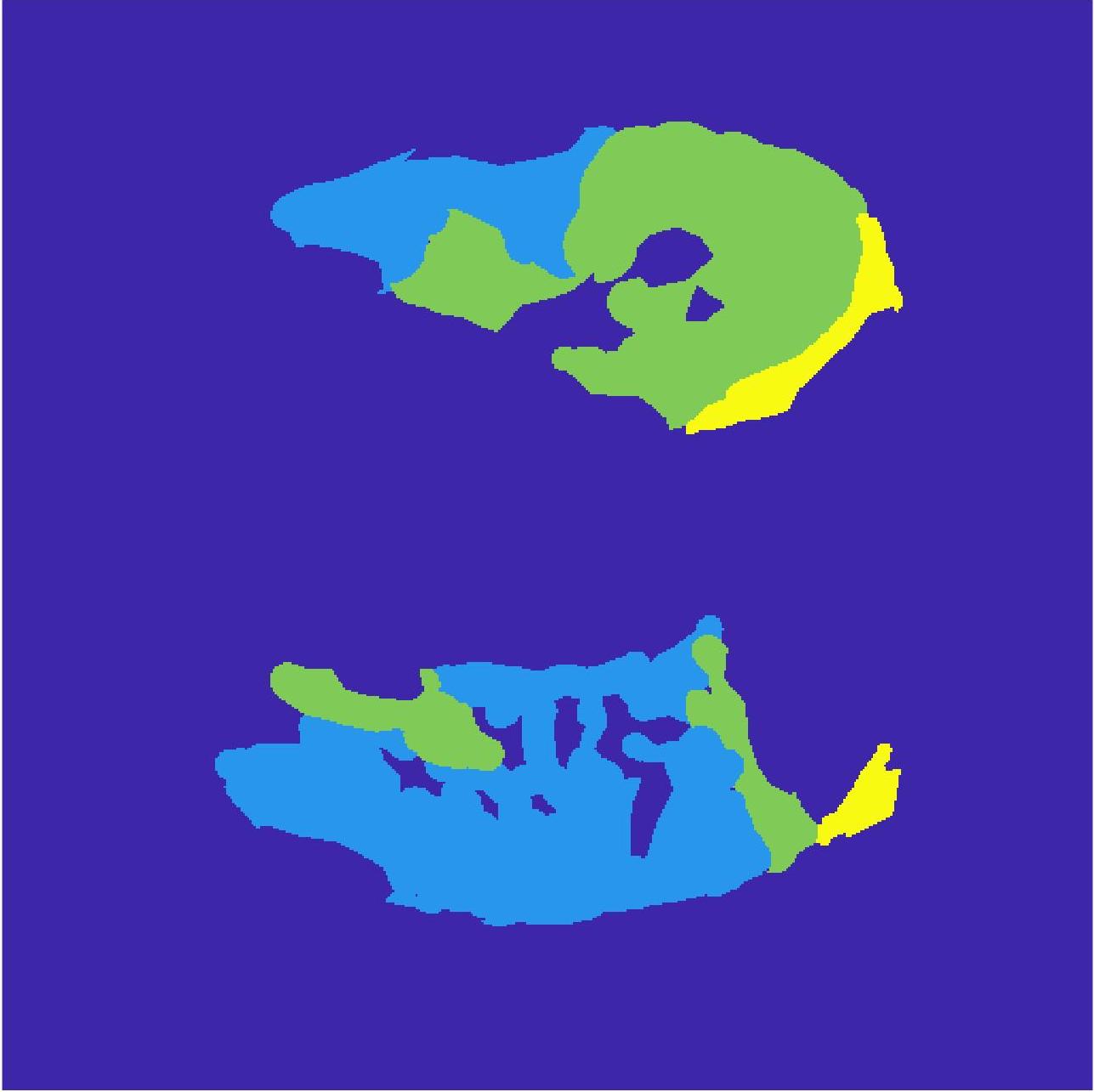
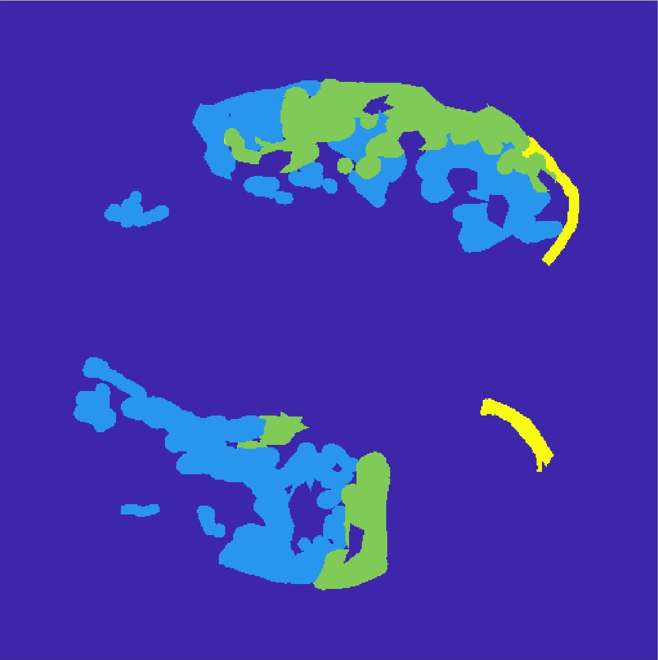
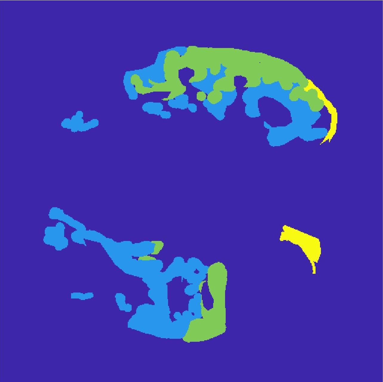
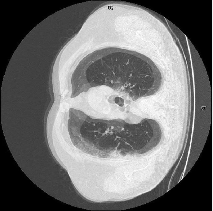
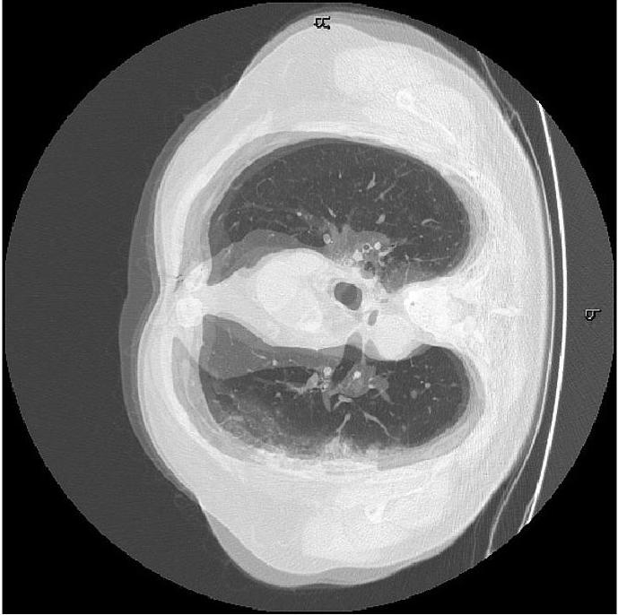
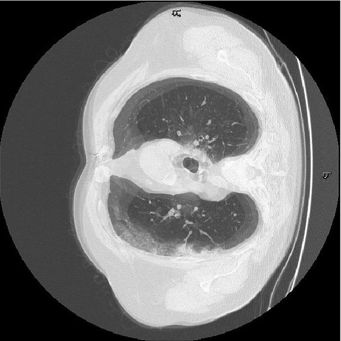
Table IV shows the segmentation results for different ablation studies. Figure 8 shows the segmentation mask obtained by different baselines for the same image shown in Figure 7 (a). The segmentation outputs are quite different from the ground truth and the one obtained by GeoGAN. In some cases the normal regions in the layers are included as pathological area, while parts of the infected region are not segmented with the pathological region. Either case is undesirable for disease diagnosis and quantification. Thus, different components of our cost functions are integral to the method’s performance and excluding one or more of classification loss, geometric loss and sampling loss adversely affects segmentation performance.

(a)	(b)	(c)

Figure 8: Segmentation results for ablation experiments on $CTSeg1$: (a) $GeoGAN_{noL_{shape}}$; (b) $GeoGAN_{noL_{cls}}$; (c) $GeoGAN_{noSamp}$. The two rows correspond to the images shown in the two rows of Figure 7 (a).

	GeoGAN	GeoGAN	GeoGAN
	${}_{noL_{cls}}$	${}_{noL_{shape}}$	noSamp
DM	0.752(0.07)	0.759(0.09)	0.758(0.09)
HD	9.5(3.0)	9.2(3.3)	9.0(3.2)
MAE	0.078	0.080	0.079
p	0.001	0.001	0.0009

TABLE IV: Mean and standard deviation (in brackets) of segmentation results from ablation studies on COVID CT images from the $CTSeg1$ database. HD is in mm. $p-$values are with respect to GeoGAN.

(a)	(b)	(c)

Figure 9: Generated images for ablation study methods: (a) $GeoGAN_{noL_{cls}}$; (b) $GeoGAN_{noL_{shape}}$; (c) $GeoGAN_{noSamp}$. The corresponding generated images for other methods are shown in Figure 2.

IV-F Classification Results

Table V summarizes the performance of different methods on the public challenge dataset of [168] consisting of $349$ CT images labeled as being COVID-19 positive. These CT images have different sizes and come from $216$ patients. All of them are resized to $512\times 512$. We train GeoGAN_WSS on the training set, generate more images, train classifiers on the training images and apply it on the test set. The leaderboard can be accessed here. For all test submissions Accuracy (ACC), F1 score (F1) and area under curve (AUC) are calculated, while the ranking is based on the F1 score. We use a DenseNet-121 architecture and employed GeoGAN_WSS augmentation for the final results. Using conventional data augmentation we got the following values: F1=0.931,ACC=0.934,AUC=0.961, which would have placed us $6^{th}$ in the current leaderboard. However, by using GeoGAN_WSS our results are ranked third although we obtain the highest AUC and ACC values, while being very close to the top ranked method in terms of F1 score. For the completeness of the paper we would have liked to report the $p-$values at 95% confidence. However we are unable to do so since we do not have access to the results of other methods.

	Rank 1	Rank 2	Rank 3	Rank 4	Rank 5
			(GeoGANWSS)
ACC	0.939	0.953	0.961	0.956	0.945
F1	0.967	0.964	0.963	0.953	0.943
AUC	0.965	0.987	0.991	0.987	0.946

TABLE V: Classification results on the public COVID-19 CT classification challenge dataset.

In a second set of classification experiments we used the $CTSeg1$ dataset to generate augmentation images and train a classifier for detection COVID positive and negative cases. The classifier was used to classify images from the $CTSeg2$ and $CTSeg3$ datasets. Images from the two datasets were intensity normalized and combined into one dataset. We add COVID negative images from the challenge dataset to get an almost equal distribution of positive and negative cases in the training and test sets. The classification results on the test set are summarized in Table VI for DenseNet-121, and Table VII for ResNet-50.

An important component of our method is the WSS step which generates segmentation maps for a given image. For the classification dataset we do not have manual segmentation labels (from the challenge dataset) to verify the accuracy of our WSS method. However, the method’s performance is reflected in the final classification performance which is better than other augmentation methods.

	GeoGAN	[166]	DAGAN	cGAN	GeoGANwClass	GeoGANwShape	GeoGANwSamp
Spe	0.931	0.916	0.893	0.881	0.873	0.869	0.877
	(0.023)	(0.028)	(0.031)	(0.024)	(0.030)	(0.035)	(0.038)
Sen	0.942	0.923	0.906	0.890	0.884	0.882	0.890
	(0.031)	(0.029)	(0.036)	(0.033)	(0.029)	(0.031)	(0.035)
Acc	0.938	0.920	0.902	0.887	0.881	0.877	0.886
	(0.026)	(0.030)	(0.033)	(0.036)	(0.032)	(0.034)	(0.034)
AUC	0.967	0.946	0.928	0.917	0.912	0.904	0.911
	(0.019)	(0.023)	(0.026)	(0.025)	(0.027)	(0.031)	(0.033)

TABLE VI: Classification results using the DenseNet-121 architecture. Values indicate mean(standard deviation). The best results are highlighted in bold.

	GeoGAN	[166]	DAGAN	cGAN	GeoGANwClass	GeoGANwShape	GeoGANwSamp
Spe	0.915	0.901	0.864	0.857	0.849	0.842	0.850
	(0.037)	(0.039)	(0.042)	(0.044)	(0.041)	(0.046)	(0.048)
Sen	0.924	0.907	0.872	0.864	0.855	0.851	0.858
	(0.036)	(0.040)	(0.041)	(0.045)	(0.043)	(0.047)	(0.046)
Acc	0.921	0.906	0.869	0.862	0.853	0.848	0.855
	(0.032)	(0.037)	(0.039)	(0.041)	(0.038)	(0.043)	(0.042)
AUC	0.943	0.927	0.887	0.883	0.876	0.870	0.877
	(0.024)	(0.028)	(0.029)	(0.031)	(0.035)	(0.034)	(0.035)

TABLE VII: Classification results using the ResNet-50 architecture. Values indicate mean(standard deviation). The best results are highlighted in bold.

V Conclusion

We propose a novel approach to generate plausible COVID-19 CT images by incorporating relationship between segmentation labels to guide the shape generation process. Diversity is introduced in the image generation process through uncertainty sampling. Comparative results show that the augmented dataset from $GeoGAN$ outperforms standard data augmentation and other competing methods, when applied to segmentation of COVID-19 affected pathological regions in CT images. We show that synergy between shape, classification and sampling terms lead to improved segmentation and each of these terms is equally important in generating realistic shapes.

Despite the good performance of our method we observe failure cases when the base images are noisy due to inherent characteristics of the image acquisition procedure. Our method is also useful to generate realistic images for educating clinicians, where targeted synthetic images (e.g. generation of complex cases, or disease mimickers) can be used to speed-up training.

References

- [1] Antreas Antoniou, Amos Storkey, and Harrison Edwards. Data augmentation generative adversarial networks. In arXiv preprint arXiv:1711.04340,, 2017.
- [2] BJ Antony, S Sedai, D Mahapatra, and R Garnavi. Real-time passive monitoring and assessment of pediatric eye health. In US Patent App. 16/178,757, 2020.
- [3] P.R. Bastide, I.F. Kiral-Kornek, D. Mahapatra, S. Saha, A. Vishwanath, and S. Von Cavallar. Machine learned optimizing of health activity for participants during meeting times. In US Patent App. 15/426,634, 2018.
- [4] P.R. Bastide, I.F. Kiral-Kornek, D. Mahapatra, S. Saha, A. Vishwanath, and S. Von Cavallar. Visual health maintenance and improvement. In US Patent 9,993,385, 2018.
- [5] P.R. Bastide, I.F. Kiral-Kornek, D. Mahapatra, S. Saha, A. Vishwanath, and S. Von Cavallar. Crowdsourcing health improvements routes. In US Patent App. 15/611,519, 2019.
- [6] Christian F. Baumgartner, Kerem C. Tezcan, Krishna Chaitanya, Andreas M. Hötker, Urs J. Muehlematter, Khoschy Schawkat, Anton S. Becker, Olivio Donati, and Ender Konukoglu. Phiseg: Capturing uncertainty in medical image segmentation. In Proc. MICCAI(2), pages 119–127, 2019.
- [7] Fred L. Bookstein. Integration, disintegration, and self-similarity: Characterizing the scales of shape variation in landmark data. Evolutionary Biology, 42(4):395–426, 2015.
- [8] B. Bozorgtabar, D. Mahapatra, and J-P. Thiran. Exprada: Adversarial domain adaptation for facial expression analysis. In Press Pattern Recognition, 100:15–28, 2020.
- [9] B. Bozorgtabar, D. Mahapatra, J.-P. Thiran, and L. Shao. SALAD: Self-supervised aggregation learning for anomaly detection on x-rays. In In Proc. MICCAI, pages 468–478, 2020.
- [10] B. Bozorgtabar, D. Mahapatra, H. von Teng, A. Pollinger, L. Ebner, J-P. Thiran, and M. Reyes. Informative sample generation using class aware generative adversarial networks for classification of chest xrays. Computer Vision and Image Understanding, 184:57–65, 2019.
- [11] Behzad Bozorgtabar, Dwarikanath Mahapatra, Hendrik von Teng, Alexander Pollinger, Lucas Ebner, Jean-Philipe Thiran, and Mauricio Reyes. Informative sample generation using class aware generative adversarial networks for classification of chest xrays. Computer Vision and Image Understanding, 184:57–65, 2019.
- [12] B. Bozorgtabar, D. Mahapatra, H. von Teng, A. Pollinger, L. Ebner, J-P. Thiran, and M. Reyes. Informative sample generation using class aware generative adversarial networks for classification of chest xrays. In arXiv preprint arXiv:1904.10781, 2019.
- [13] B. Bozorgtabar, D. Mahapatra, G. Vray, and J.-P. Thiran. Anomaly detection on x-rays using self-supervised aggregation learning. In arXiv preprint arXiv:2010.09856, 2020.
- [14] B. Bozorgtabar, D. Mahapatra, I. Zlobec, T.T. Rau, and J.P. Thiran. Computational pathology. Frontiers in Medicine, 7, 2020.
- [15] B. Bozorgtabar, M. Saeed Rad, D. Mahapatra, and J-P. Thiran. Syndemo: Synergistic deep feature alignment for joint learning of depth and ego-motion. In In Proc. IEEE ICCV, 2019.
- [16] S. Chaganti, A. Balachandran, and et. al. Quantification of tomographic patterns associated with covid-19 from chest ct. In arXiv, 2020.
- [17] J. Chen, L. Wu, and et al. Deep learning-based model for detecting 2019 novel coronavirus pneumonia on high-resolution computed tomography: a prospective study. In medRxiv, 2020.
- [18] Alexey Dosovitskiy, Philipp Fischer, Jost Tobias Springenberg, Martin Riedmiller, and Thomas Brox. Discriminative unsupervised feature learning with exemplar convolutional neural networks. IEEE Trans. Patt. Anal. Mach. Intell., 38(9):1734–1747, 2016.
- [19] Deng-Ping Fan, Tao Zhou, Ge-Peng Ji, Yi Zhou, Geng Chen, Huazhu Fu, Jianbing Shen, and Ling Shao. Inf-net: Automatic covid-19 lung infection segmentation from ct scans. arXiv preprint arXiv:2004.14133, 2020.
- [20] R Garnavi, D Mahapatra, PK Roy, and RB Tennakoon. System and method to teach and evaluate image grading performance using prior learned expert knowledge base. In US Patent App. 10,657,838, 2020.
- [21] Z. Ge, D. Mahapatra, X. Chang, Z. Chen, L. Chi, and H. Lu. Improving multi-label chest x-ray disease diagnosis by exploiting disease and health labels dependencies. In press Multimedia Tools and Application, pages 1–14, 2019.
- [22] Z. Ge, D. Mahapatra, S. Sedai, R. Garnavi, and R. Chakravorty. Chest x-rays classification: A multi-label and fine-grained problem. In arXiv preprint arXiv:1807.07247, 2018.
- [23] Ian Goodfellow, Jean Pouget-Abadie, Mehdi Mirza, Bing Xu, David Warde-Farley, Sherjil Ozair, Aaron Courville, and Yoshua Bengio. Generative adversarial nets. In Advances in neural information processing systems, pages 2672–2680, 2014.
- [24] P. M. Gordaliza, A. Munoz-Barrutia, M. Abella, M. Desco, S. Sharpe, and J. J. Vaquero. Unsupervised ct lung image segmentation of a mycobacterium tuberculosis infection model. Scientific Reports, 8(1):1–10, 2018.
- [25] Changhee Han, Hideaki Hayashi, Leonardo Rundo, Ryosuke Araki, Wataru Shimoda, Shinichi Muramatsu, Yujiro Furukawa, Giancarlo Mauri, and Hideki Nakayama. Gan-based synthetic brain mr image generation. In 2018 IEEE 15th International Symposium on Biomedical Imaging (ISBI 2018), pages 734–738. IEEE, 2018.
- [26] J De Hoog, D Mahapatra, R Garnavi, and F Jalali. Personalized monitoring of injury rehabilitation through mobile device imaging. In US Patent App. 16/589,046, 2021.
- [27] C. Huang, Y. Wang, and et al. Clinical features of patients infected with 2019 novel coronavirus in wuhan, china,. The Lancet, 395(10223):497–506, 2020.
- [28] C. Huang, Y. Wang, and et al. Clinical features of patients infected with 2019 novel coronavirus in wuhan, china,. The Lancet, 395(10223):497–506, 2020.
- [29] Max Jaderberg, Karen Simonyan, Andrew Zisserman, and Koray Kavukcuoglu. Spatial transformer networks. In NIPS, pages –, 2015.
- [30] J. Jian, Y.-C. Hu, and et. al. Multiple resolution residually connected feature streams for automatic lung tumor segmentation from ct images. IEEE Trans. Med. Imag., 38(1):134–144, 2018.
- [31] D. Jin, Z. Xu, Y. Tang, A. P. Harrison, and D. J. Mollura. Ct-realistic lung nodule simulation from 3d conditional generative adversarial networks for robust lung segmentation. In Proc. MICCAI, pages 732–740, 2018.
- [32] L Ju, X Wang, L Wang, T. Liu, X. Zhao, T. Drummond, D. Mahapatra, and Z. Ge. Relational subsets knowledge distillation for long-tailed retinal diseases recognition. In arXiv preprint arXiv:2104.11057, 2021.
- [33] L Ju, X Wang, L Wang, D Mahapatra, X Zhao, M Harandi, T Drummond, Tongliang Liu, and Zongyuan Ge. Improving medical image classification with label noise using dual-uncertainty estimation. In arXiv preprint arXiv:2103.00528, 2020.
- [34] Lie Ju, Xin Wang, Xin Zhao, Huimin Lu, Dwarikanath Mahapatra, Paul Bonnington, and Zongyuan Ge. Synergic adversarial label learning for grading retinal diseases via knowledge distillation and multi-task learning. IEEE JBHI, 100:1–14, 2020.
- [35] Alex Kendall, Vijay Badrinarayanan, and Roberto Cipolla. Bayesian segnet: Model uncertainty in deep convolutional encoder-decoder architectures for scene understanding. In arXiv:1511.02680, 2015.
- [36] M. Keshani, Z. Azimifar, F. Tajeripour, and R. Boostani. Lung nodule segmentation and recognition using svm classifier and active contour modeling: A complete intelligent system. Computers in Biology and Medicine, 43(4):287–300, 2013.
- [37] Diederik P. Kingma and Jimmy Ba. Adam: A method for stochastic optimization. In arXiv preprint arXiv:1412.6980,, 2014.
- [38] Simon A. A. Kohl, Bernardino Romera-Paredes, Clemens Meyer, Jeffrey De Fauw, Joseph R. Ledsam, Klaus H. Maier-Hein, S. M. Ali Eslami, Danilo Jimenez Rezende, and Olaf Ronneberger. A probabilistic u-net for segmentation of ambiguous images. In Proc. NIPS, pages 6965–6975, 2018.
- [39] S. Kuanar, V. Athitsos, D. Mahapatra, and A. Rajan. Multi-scale deep learning architecture for nucleus detection in renal cell carcinoma microscopy image. In arXiv preprint arXiv:2104.13557, 2021.
- [40] S. Kuanar, V Athitsos, D. Mahapatra, K.R. Rao, Z. Akhtar, and D. Dasgupta. Low dose abdominal ct image reconstruction: An unsupervised learning based approach. In In Proc. IEEE ICIP, pages 1351–1355, 2019.
- [41] Shiba Kuanar, Dwarikanath Mahapatra, Monalisa Bilas, and KR Rao. Multi-path dilated convolution network for haze and glow removal in night time images. The Visual Computer, pages 1–14, 2021.
- [42] S. Kuanar, K.R. Rao, D. Mahapatra, and M. Bilas. Night time haze and glow removal using deep dilated convolutional network. In arXiv preprint arXiv:1902.00855, 2019.
- [43] H. Kuang, B. Guthier, M. Saini, D. Mahapatra, and A. El Saddik. A real-time smart assistant for video surveillance through handheld devices. In In Proc: ACM Intl. Conf. Multimedia, pages 917–920, 2014.
- [44] Balaji Lakshminarayanan, Alexander Pritzel, and Charles Blundell. Simple and scalable predictive uncertainty estimation using deep ensembles. In Proc. NIPS, pages 6402–6413, 2017.
- [45] Kelvin K. Leung, Matthew J. Clarkson, Johnathon W. Bartlett, Shona Clegg, Clifford R. Jack Jr, Michael W. Weiner, Nick C. Fox, Sebastien Ourselin, and A. D. N. Initiative. Robust atrophy rate measurement in alzheimer’s disease using multi-site serial mri: tissue-specific intensity normalization and parameter selection. Neuroimage, 50(2):516–523, 2010.
- [46] Z. Li, D. Mahapatra, J.Tielbeek, J. Stoker, L. van Vliet, and F.M. Vos. Image registration based on autocorrelation of local structure. IEEE Trans. Med. Imaging, 35(1):63–75, 2016.
- [47] D. Mahapatra. Neonatal brain mri skull stripping using graph cuts and shape priors. In In Proc: MICCAI workshop on Image Analysis of Human Brain Development (IAHBD), 2011.
- [48] Dwarikanath Mahapatra. Registration and segmentation methodology for perfusion mr images: Application to cardiac and renal images. -, pages –, 2011.
- [49] D. Mahapatra. Cardiac lv and rv segmentation using mutual context information. In Proc. MICCAI-MLMI, pages 201–209, 2012.
- [50] D. Mahapatra. Groupwise registration of dynamic cardiac perfusion images using temporal information and segmentation information. In In Proc: SPIE Medical Imaging, 2012.
- [51] D. Mahapatra. Landmark detection in cardiac mri using learned local image statistics. In Proc. MICCAI-Statistical Atlases and Computational Models of the Heart. Imaging and Modelling Challenges (STACOM), pages 115–124, 2012.
- [52] D. Mahapatra. Skull stripping of neonatal brain mri: Using prior shape information with graphcuts. J. Digit. Imaging, 25(6):802–814, 2012.
- [53] D. Mahapatra. Cardiac image segmentation from cine cardiac mri using graph cuts and shape priors. J. Digit. Imaging, 26(4):721–730, 2013.
- [54] D. Mahapatra. Cardiac mri segmentation using mutual context information from left and right ventricle. J. Digit. Imaging, 26(5):898–908, 2013.
- [55] D. Mahapatra. Graph cut based automatic prostate segmentation using learned semantic information. In Proc. IEEE ISBI, pages 1304–1307, 2013.
- [56] D. Mahapatra. Joint segmentation and groupwise registration of cardiac perfusion images using temporal information. J. Digit. Imaging, 26(2):173–182, 2013.
- [57] D. Mahapatra. Automatic cardiac segmentation using semantic information from random forests. J. Digit. Imaging., 27(6):794–804, 2014.
- [58] D. Mahapatra. Combining multiple expert annotations using semi-supervised learning and graph cuts for medical image segmentation. Computer Vision and Image Understanding, 151(1):114–123, 2016.
- [59] D. Mahapatra. Consensus based medical image segmentation using semi-supervised learning and graph cuts. In arXiv preprint arXiv:1612.02166, 2017.
- [60] D. Mahapatra. Semi-supervised learning and graph cuts for consensus based medical image segmentation. Pattern Recognition, 63(1):700–709, 2017.
- [61] D. Mahapatra. Amd severity prediction and explainability using image registration and deep embedded clustering. In arXiv preprint arXiv:1907.03075, 2019.
- [62] D. Mahapatra. Registration of histopathogy images using structural information from fine grained feature maps. In arXiv preprint arXiv:2007.02078, 2020.
- [63] D. Mahapatra. Interpretability-driven sample selection using self supervised learning for disease classification and segmentation. In arXiv preprint arXiv:2104.06087, 2021.
- [64] D. Mahapatra, K. Agarwal, R. Khosrowabadi, and D.K. Prasad. Recent advances in statistical data and signal analysis: Application to real world diagnostics from medical and biological signals. In Computational and mathematical methods in medicine, 2016.
- [65] D. Mahapatra, B. Antony, S. Sedai, and R. Garnavi. Deformable medical image registration using generative adversarial networks. In In Proc. IEEE ISBI, pages 1449–1453, 2018.
- [66] D. Mahapatra and B. Bozorgtabar. Retinal vasculature segmentation using local saliency maps and generative adversarial networks for image super resolution. In arXiv preprint arXiv:1710.04783, 2017.
- [67] D. Mahapatra and B. Bozorgtabar. Progressive generative adversarial networks for medical image super resolution. In arXiv preprint arXiv:1902.02144, 2019.
- [68] D. Mahapatra, B. Bozorgtabar, and R. Garnavi. Image super-resolution using progressive generative adversarial networks for medical image analysis. Computerized Medical Imaging and Graphics, 71:30–39, 2019.
- [69] D. Mahapatra, B. Bozorgtabar, and J.-P. Thiran L. Shao. Pathological retinal region segmentation from oct images using geometric relation based augmentation. In arXiv preprint arXiv:2003.14119, 2020.
- [70] D. Mahapatra, B. Bozorgtabar, and L. Shao. Pathological retinal region segmentation from oct images using geometric relation based augmentation. In In Proc. IEEE CVPR, pages 9611–9620, 2020.
- [71] Dwarikanath Mahapatra, Behzad Bozorgtabar, Jean-Phillipe Thiran, and Mauricio Reyes. Efficient active learning for image classification and segmentation using a sample selection and conditional generative adversarial network. In MICCAI, pages 580–588, 2018.
- [72] D. Mahapatra, B. Bozorgtabar, J.-P. Thiran, and L. Shao. Structure preserving stain normalization of histopathology images using self supervised semantic guidance. In In Proc. MICCAI, pages 309–319, 2020.
- [73] D. Mahapatra, B. Bozorgtabar, J.-P. Thiran, and L. Shao. Structure preserving stain normalization of histopathology images using self supervised semantic guidance. In arXiv preprint arXiv:2008.02101, 2020.
- [74] D. Mahapatra, S. Bozorgtabar, S. Hewavitahranage, and R. Garnavi. Image super resolution using generative adversarial networks and local saliencymaps for retinal image analysis,. In In Proc. MICCAI, pages 382–390, 2017.
- [75] D. Mahapatra, S. Bozorgtabar, J.-P. Thiran, and M. Reyes. Efficient active learning for image classification and segmentation using a sample selection and conditional generative adversarial network. In In Proc. MICCAI (2), pages 580–588, 2018.
- [76] D. Mahapatra and J.M. Buhmann. Automatic cardiac rv segmentation using semantic information with graph cuts. In Proc. IEEE ISBI, pages 1094–1097, 2013.
- [77] D. Mahapatra and J.M. Buhmann. Analyzing training information from random forests for improved image segmentation. IEEE Trans. Imag. Proc., 23(4):1504–1512, 2014.
- [78] D. Mahapatra and J.M. Buhmann. Prostate mri segmentation using learned semantic knowledge and graph cuts. IEEE Trans. Biomed. Engg., 61(3):756–764, 2014.
- [79] D. Mahapatra and J.M. Buhmann. A field of experts model for optic cup and disc segmentation from retinal fundus images. In In Proc. IEEE ISBI, pages 218–221, 2015.
- [80] D. Mahapatra and J. Buhmann. Obtaining consensus annotations for retinal image segmentation using random forest and graph cuts. In In Proc. OMIA, pages 41–48, 2015.
- [81] D. Mahapatra and J. Buhmann. Visual saliency based active learning for prostate mri segmentation. In In Proc. MLMI, pages 9–16, 2015.
- [82] D. Mahapatra and J. Buhmann. Visual saliency based active learning for prostate mri segmentation. SPIE Journal of Medical Imaging, 3(1), 2016.
- [83] D. Mahapatra, R Garnavi, P.K. Roy, and R.B. Tennakoon. System and method to teach and evaluate image grading performance using prior learned expert knowledge base. In US Patent App. 15/459,457, 2018.
- [84] D. Mahapatra, R Garnavi, P.K. Roy, and R.B. Tennakoon. System and method to teach and evaluate image grading performance using prior learned expert knowledge base. In US Patent App. 15/814,590, 2018.
- [85] D. Mahapatra, R Garnavi, S. Sedai, and P.K. Roy. Joint segmentation and characteristics estimation in medical images. In US Patent App. 15/234,426, 2017.
- [86] D. Mahapatra, R Garnavi, S. Sedai, and P.K. Roy. Retinal image quality assessment, error identification and automatic quality correction. In US Patent 9,779,492, 2017.
- [87] D. Mahapatra, R Garnavi, S. Sedai, and R.B. Tennakoon. Classification of severity of pathological condition using hybrid image representation. In US Patent App. 15/426,634, 2018.
- [88] D. Mahapatra, R Garnavi, S. Sedai, and R.B. Tennakoon. Generating an enriched knowledge base from annotated images. In US Patent App. 15/429,735, 2018.
- [89] D. Mahapatra, R Garnavi, S. Sedai, R.B. Tennakoon, and R. Chakravorty. Early prediction of age related macular degeneration by image reconstruction. In US Patent App. 15/854,984, 2018.
- [90] D. Mahapatra, R Garnavi, S. Sedai, R.B. Tennakoon, and R. Chakravorty. Early prediction of age related macular degeneration by image reconstruction. In US Patent 9,943,225, 2018.
- [91] D. Mahapatra and Z. Ge. Combining transfer learning and segmentation information with gans for training data independent image registration. In arXiv preprint arXiv:1903.10139, 2019.
- [92] D. Mahapatra and Z. Ge. Training data independent image registration with gans using transfer learning and segmentation information. In In Proc. IEEE ISBI, pages 709–713, 2019.
- [93] D. Mahapatra and Z. Ge. Training data independent image registration using generative adversarial networks and domain adaptation. Pattern Recognition, 100:1–14, 2020.
- [94] D. Mahapatra, Z. Ge, and S. Sedai. Joint registration and segmentation of images using deep learning. In US Patent App. 16/001,566, 2019.
- [95] D. Mahapatra, Z. Ge, S. Sedai, and R. Chakravorty. Joint registration and segmentation of xray images using generative adversarial networks. In In Proc. MICCAI-MLMI, pages 73–80, 2018.
- [96] D. Mahapatra, S. Gilani, and M.K. Saini. Coherency based spatio-temporal saliency detection for video object segmentation. IEEE Journal of Selected Topics in Signal Processing., 8(3):454–462, 2014.
- [97] D. Mahapatra, J.Tielbeek, J.C. Makanyanga, J. Stoker, S.A. Taylor, F.M. Vos, and J.M. Buhmann. Automatic detection and segmentation of crohn’s disease tissues from abdominal mri. IEEE Trans. Med. Imaging, 32(12):1232–1248, 2013.
- [98] D. Mahapatra, J.Tielbeek, J.C. Makanyanga, J. Stoker, S.A. Taylor, F.M. Vos, and J.M. Buhmann. Active learning based segmentation of crohn’s disease using principles of visual saliency. In Proc. IEEE ISBI, pages 226–229, 2014.
- [99] D. Mahapatra, J.Tielbeek, J.C. Makanyanga, J. Stoker, S.A. Taylor, F.M. Vos, and J.M. Buhmann. Combining multiple expert annotations using semi-supervised learning and graph cuts for crohn’s disease segmentation. In In Proc: MICCAI-ABD, 2014.
- [100] D. Mahapatra, J.Tielbeek, F.M. Vos, and J.M. Buhmann. A supervised learning approach for crohn’s disease detection using higher order image statistics and a novel shape asymmetry measure. J. Digit. Imaging, 26(5):920–931, 2013.
- [101] D. Mahapatra, Z. Li, F.M. Vos, and J.M. Buhmann. Joint segmentation and groupwise registration of cardiac dce mri using sparse data representations. In In Proc. IEEE ISBI, pages 1312–1315, 2015.
- [102] Dwarikanath Mahapatra, Alexander Poellinger, Ling Shao, and Mauricio Reyes. Interpretability-driven sample selection using self supervised learning for disease classification and segmentation. IEEE TMI, pages 1–15, 2021.
- [103] D. Mahapatra, A. Routray, and C. Mishra. An active snake model for classification of extreme emotions. In IEEE International Conference on Industrial Technology (ICIT), pages 2195–2199, 2006.
- [104] D. Mahapatra, P.K. Roy, S. Sedai, and R. Garnavi. A cnn based neurobiology inspired approach for retinal image quality assessment. In In Proc. EMBC, pages 1304–1307, 2016.
- [105] D. Mahapatra, P.K. Roy, S. Sedai, and R. Garnavi. Retinal image quality classification using saliency maps and cnns. In In Proc. MICCAI-MLMI, pages 172–179, 2016.
- [106] D. Mahapatra, S. Roy, and Y. Sun. Retrieval of mr kidney images by incorporating spatial information in histogram of low level features. In In 13th International Conference on Biomedical Engineering, 2008.
- [107] D. Mahapatra, S. Saha, A. Vishwanath, and P.R. Bastide. Generating hyperspectral image database by machine learning and mapping of color images to hyperspectral domain. In US Patent App. 15/949,528, 2019.
- [108] D. Mahapatra, M.K. Saini, and Y. Sun. Illumination invariant tracking in office environments using neurobiology-saliency based particle filter. In IEEE ICME, pages 953–956, 2008.
- [109] D. Mahapatra, P. Schffler, J. Tielbeek, F.M. Vos, and J.M. Buhmann. Semi-supervised and active learning for automatic segmentation of crohn’s disease. In Proc. MICCAI, Part 2, pages 214–221, 2013.
- [110] D. Mahapatra, S. Sedai, and R. Garnavi. Elastic registration of medical images with gans. In arXiv preprint arXiv:1805.02369, 2018.
- [111] D. Mahapatra, S. Sedai, and K. Halupka. Uncertainty region based image enhancement. In US Patent App. 10,832,074, 2020.
- [112] D. Mahapatra and Y. Sun. Nonrigid registration of dynamic renal MR images using a saliency based MRF model. In Proc. MICCAI, pages 771–779, 2008.
- [113] D. Mahapatra and Y. Sun. Registration of dynamic renal mr images using neurobiological model of saliency. In Proc. ISBI, pages 1119–1122, 2008.
- [114] D. Mahapatra and Y. Sun. Using saliency features for graphcut segmentation of perfusion kidney images. In In 13th International Conference on Biomedical Engineering, 2008.
- [115] D. Mahapatra and Y. Sun. Joint registration and segmentation of dynamic cardiac perfusion images using mrfs. In Proc. MICCAI, pages 493–501, 2010.
- [116] D. Mahapatra and Y. Sun. An mrf framework for joint registration and segmentation of natural and perfusion images. In Proc. IEEE ICIP, pages 1709–1712, 2010.
- [117] D. Mahapatra and Y. Sun. Retrieval of perfusion images using cosegmentation and shape context information. In Proc. APSIPA Annual Summit and Conference (ASC), 2010.
- [118] D. Mahapatra and Y. Sun. Rigid registration of renal perfusion images using a neurobiology based visual saliency model. EURASIP Journal on Image and Video Processing., pages 1–16, 2010.
- [119] D. Mahapatra and Y. Sun. A saliency based mrf method for the joint registration and segmentation of dynamic renal mr images. In Proc. ICDIP, 2010.
- [120] D. Mahapatra and Y. Sun. Mrf based intensity invariant elastic registration of cardiac perfusion images using saliency information. IEEE Trans. Biomed. Engg., 58(4):991–1000, 2011.
- [121] D. Mahapatra and Y. Sun. Orientation histograms as shape priors for left ventricle segmentation using graph cuts. In In Proc: MICCAI, pages 420–427, 2011.
- [122] D. Mahapatra and Y. Sun. Integrating segmentation information for improved mrf-based elastic image registration. IEEE Trans. Imag. Proc., 21(1):170–183, 2012.
- [123] D. Mahapatra, J. Tielbeek, J.M. Buhmann, and F.M. Vos. A supervised learning based approach to detect crohn’s disease in abdominal mr volumes. In Proc. MICCAI workshop Computational and Clinical Applications in Abdominal Imaging(MICCAI-ABD), pages 97–106, 2012.
- [124] D. Mahapatra, J. Tielbeek, F.M. Vos, and J.M. Buhmann . Crohn’s disease tissue segmentation from abdominal mri using semantic information and graph cuts. In Proc. IEEE ISBI, pages 358–361, 2013.
- [125] D. Mahapatra, J. Tielbeek, F.M. Vos, and J.M. Buhmann. Localizing and segmenting crohn’s disease affected regions in abdominal mri using novel context features. In Proc. SPIE Medical Imaging, 2013.
- [126] D. Mahapatra, J. Tielbeek, F.M. Vos, and J.M. Buhmann. Weakly supervised semantic segmentation of crohn’s disease tissues from abdominal mri. In Proc. IEEE ISBI, pages 832–835, 2013.
- [127] D. Mahapatra, F.M. Vos, and J.M. Buhmann. Crohn’s disease segmentation from mri using learned image priors. In In Proc. IEEE ISBI, pages 625–628, 2015.
- [128] D. Mahapatra, F.M. Vos, and J.M. Buhmann. Active learning based segmentation of crohns disease from abdominal mri. Computer Methods and Programs in Biomedicine, 128(1):75–85, 2016.
- [129] D. Mahapatra, S. Winkler, and S.C. Yen. Motion saliency outweighs other low-level features while watching videos. In SPIE HVEI., pages 1–10, 2008.
- [130] Fausto Milletari, Nassir Navab, and Seyed-Ahmad Ahmadi. V-net: Fully convolutional neural networks for volumetric medical im- age segmentation. In Proc. Int. Conf. on 3D vision, pages 565–571, 2016.
- [131] Christopher Nielsen and Michal Okoniewski. Gan data augmentation through active learning inspired sample acquisition. In Proceedings of the IEEE Conference on Computer Vision and Pattern Recognition Workshops, pages 109–112, 2019.
- [132] V. Rajinikanth, N. Dey, and et al. Harmony-search and otsu based system for coronavirus disease (covid-19) detection using lung ct scan images,. https://arxiv.org/abs/2004.03431. Online; accessed 15 May 2020.
- [133] Olaf Ronneberger, Phillip Fischer, and Thomas Brox. U-net: Convolutional networks for biomedical image segmentation. In In Proc. MICCAI, pages 234–241, 2015.
- [134] P. Roy, R. Chakravorty, S. Sedai, D. Mahapatra, and R. Garnavi. Automatic eye type detection in retinal fundus image using fusion of transfer learning and anatomical features. In In Proc. DICTA, pages 1–7, 2016.
- [135] P.K. Roy, D. Mahapatra, R. Garnavi, and R.B. Tennakoon. System and method to teach and evaluate image grading performance using prior learned expert knowledge base. In US Patent App. 10,984,674, 2021.
- [136] P. Roy, R. Tennakoon, K. Cao, S. Sedai, D. Mahapatra, S. Maetschke, and R. Garnavi. A novel hybrid approach for severity assessment of diabetic retinopathy in colour fundus images,. In In Proc. IEEE ISBI, pages 1078–1082, 2017.
- [137] G. D. Rubin, L. B. Haramati, and et al. The role of chest imaging in patient management during the covid-19 pandemic: A multinational consensus statement from the fleischner society. Radiology, 201365, 2020.
- [138] Christian Rupprecht, Iro Laina, Robert DiPietro, Maximilian Baust, Federico Tombari, Nassir Navab, and Gregory D. Hager. Learning in an uncertain world: Representing ambiguity through multiple hypotheses. In Proc. CVPR, pages 3591–3600, 2017.
- [139] M. Saini, B. Guthier, H. Kuang, D. Mahapatra, and A.E. Saddik. szoom: A framework for automatic zoom into high resolution surveillance videos. In arXiv preprint arXiv:1909.10164, 2019.
- [140] P. Schffler, D. Mahapatra, J. Tielbeek, F.M. Vos, J. Makanyanga, D.A. Pends, C.Y. Nio, J. Stoker, S.A. Taylor, and J.M. Buhmann. A model development pipeline for crohns disease severity assessment from magnetic resonance images. In In Proc: MICCAI-ABD, 2013.
- [141] P. Schffler, D. Mahapatra, J. Tielbeek, F.M. Vos, J. Makanyanga, D.A. Pends, C.Y. Nio, J. Stoker, S.A. Taylor, and J.M. Buhmann. Semi automatic crohns disease severity assessment on mr imaging. In In Proc: MICCAI-ABD, 2014.
- [142] S. Sedai, D. Mahapatra, B. Antony, and R. Garnavi. Joint segmentation and uncertainty visualization of retinal layers in optical coherence tomography images using bayesian deep learning. In In Proc. MICCAI-OMIA, pages 219–227, 2018.
- [143] S. Sedai, D. Mahapatra, Z. Ge, R. Chakravorty, and R. Garnavi. Deep multiscale convolutional feature learning for weakly supervised localization of chest pathologies in x-ray images. In In Proc. MICCAI-MLMI, pages 267–275, 2018.
- [144] S. Sedai, D. Mahapatra, S. Hewavitharanage, S. Maetschke, and R. Garnavi. Semi-supervised segmentation of optic cup in retinal fundus images using variational autoencoder,. In In Proc. MICCAI, pages 75–82, 2017.
- [145] S. Sedai, P.K. Roy, D. Mahapatra, and R. Garnavi. Segmentation of optic disc and optic cup in retinal fundus images using shape regression. In In Proc. EMBC, pages 3260–3264, 2016.
- [146] S. Sedai, P.K. Roy, D. Mahapatra, and R. Garnavi. Segmentation of optic disc and optic cup in retinal images using coupled shape regression. In In Proc. MICCAI-OMIA, pages 1–8, 2016.
- [147] F. Shan, Y. Gao, and et. al. Lung infection quantification of covid-19 in ct images with deep learning. In arXiv, 2020.
- [148] F. Shi, J. Wang, and et al. Review of artificial intelligence techniques in imaging data acquisition, segmentation and diagnosis for covid-19. https://arxiv.org/abs/2004.02731. Online; accessed 15 May 2020.
- [149] Hoo-Chang Shin, Neil A Tenenholtz, Jameson K Rogers, Christopher G Schwarz, Matthew L Senjem, Jeffrey L Gunter, Katherine Andriole, and Mark Michalski. Medical Image Synthesis for Data Augmentation and Anonymization using Generative Adversarial Networks. In Proc. MICCAI-SASHIMI, 2018.
- [150] I. Sluimer, A. Schilham, M. Prokop, and B. Van Ginneken. Computer analysis of computed tomography scans of the lung: a survey. IEEE Trans. Med. Imag., 25(4):385–405, 2006.
- [151] Kihuk Sohn, Honglak Lee, and Xinchen Yan. Learning structured output representation using deep conditional generative models. In Proc. NIPS, pages 3483–3491, 2015.
- [152] C. Szegedy, W. Liu, and et al. Going deeper with convolutions. In CVPR, pages 1–9, 2015.
- [153] R. Tennakoon, D. Mahapatra, P. Roy, S. Sedai, and R. Garnavi. Image quality classification for dr screening using convolutional neural networks. In In Proc. MICCAI-OMIA, pages 113–120, 2016.
- [154] J. Tong, D. Mahapatra, P. Bonnington, T. Drummond, and Z. Ge. Registration of histopathology images using self supervised fine grained feature maps. In In Proc. MICCAI-DART Workshop, pages 41–51, 2020.
- [155] F. M. Vos, J. Tielbeek, R. Naziroglu, Z. Li, P. Schffler, D. Mahapatra, Alexander Wiebel, C. Lavini, J. Buhmann, H. Hege, J. Stoker, and L. van Vliet. Computational modeling for assessment of IBD: to be or not to be? In Proc. IEEE EMBC, pages 3974–3977, 2012.
- [156] C. Wang, P. W. Horby, F. G. Hayden, and G. F. Gao. A novel coronavirus outbreak of global health concern. The Lancet, 395(10223):470–473, 2020.
- [157] L. Wang and A. Wong. Covid-net: A tailored deep convolutional neural network design for detection of covid-19 cases from chest radiography images,. https://arxiv.org/abs/2003.09871. Online; accessed 15 May 2020.
- [158] S. Wang, B. Kang, and et al. A deep learning algorithm using ct images to screen for corona virus disease (covid-19). In medRxiv, 2020.
- [159] S. Wang, M. Zhou, and et. al. Central focused convolutional neural networks: Developing a data-driven model for lung nodule segmentation. Medical Image Analysis, 40(1):172–183, 2017.
- [160] Y. Xing, Z. Ge, R. Zeng, D. Mahapatra, J. Seah, M. Law, and T. Drummond. Adversarial pulmonary pathology translation for pairwise chest x-ray data augmentation. In In Proc. MICCAI, pages 757–765, 2019.
- [161] G. Xu, Z. Song, Z. Sun, C. Ku, Z. Yang, C. Liu, S. Wang, J. Ma, and W. Xu. CAMEL: A weakly supervised learning framework for histopathology image segmentation. In Proc. ICCV, pages 10682–10691, 2019.
- [162] X. Xu, X. Jiang, and et. al. Deep learning system to screen coronavirus disease 2019 pneumonia. In arXiv, 2020.
- [163] Z. Ye, Y. Zhang, Y. Wang, Z. Huang, and B. Song. Chest ct manifestations of new coronavirus disease 2019 (covid-19): a pictorial review,. Eurpean Radiology, 2019(37):1–9, 2020.
- [164] Xin Yi, Ekta Walia, and Paul Babyn. Generative adversarial network in medical imaging: A review. Med. Imag. Anal., 58, 2019.
- [165] J. Zhang, Y. Xie, Y. Li, C. Shen, and Y. Xiao. Covid-19 screening on chest x-ray images using deep learning based anomaly detection. In arXiv, 2020.
- [166] Amy Zhao, Guha Balakrishnan, Fredo Durand, John V. Guttag, and Adrian V. Dalca. Data augmentation using learned transforms for one-shot medical image segmentation. In In Proc. CVPR, pages 8543–8552, 2019.
- [167] He Zhao, Huiqi Li, Sebastian Maurer-Stroh, and LiCheng. Synthesizing retinal and neuronal images with generative adversarial nets. Med. Imag. Anal, 49:14–26, 2018.
- [168] Jinyu Zhao, Yichen Zhang, Xuehai He, and Pengtao Xie. Covid-ct-dataset: a ct scan dataset about covid-19. arXiv preprint arXiv:2003.13865, 2020.
- [169] C. Zheng, X. Deng, and et. al. Deep learning-based detection for covid-19 from chest ct using weak label. In medrXiv, 2020.
- [170] Z. Zhou, M. M. R. Siddiquee, N. Tajbakhsh, and J. Liang. Unet++: Redesigning skip connections to exploit multiscale features in image segmentation. IEEE Trans. Med. Imag., pages 1–10, 2019.
- [171] J. Zilly, J. Buhmann, and D. Mahapatra. Boosting convolutional filters with entropy sampling for optic cup and disc image segmentation from fundus images. In In Proc. MLMI, pages 136–143, 2015.
- [172] J. Zilly, J.M. Buhmann, and D. Mahapatra. Glaucoma detection using entropy sampling and ensemble learning for automatic optic cup and disc segmentation. In Press Computerized Medical Imaging and Graphics, 55(1):28–41, 2017.