The most precise quantum thermoeletric

Abstract

Thermodynamic Uncertainty Relations (TURs) place lower bounds on the noise-to-signal ratio (precision) of currents in nanoscale devices. Originally formulated for classical time-homogeneous Markov processes, these relations, can be violated in quantum-coherent devices. However, the extent to which these may occur still represent a missing piece of the puzzle. In this Letter we provide the definitive answer for the class of quantum thermoelectric devices operating in the steady-state regime. Using coherent scattering theory beyond linear response, together with analytical optimization techniques, we rigorously prove that the transmission function which minimizes the variance of steady-state currents, for fixed averages, is a collection of boxcar functions. This allows us to show that TURs can be violated by arbitrarily large amounts, depending on the temperature and chemical potential gradients, thus providing guidelines to the design of optimal devices.

Introduction– The laws of thermodynamics impose a universal trade-off relation between output power, efficiency and dissipation of any heat engine. Achieving Carnot efficiency requires infinitely slow processes, with vanishing dissipation, but also zero output power. Conversely, finite power requires non-equilibrium conditions, where the efficiency is reduced and dissipation is increased Carnot (1824). However, the miniaturization march that has characterized technology over the past fifty years is pushing devices towards the meso- and nano-scale. Examples include thermoelectric engines or photovoltaic devices, able to inter-convert electrical power and heat at the microscopic level. In such systems, fluctuations become significant and represent a new ingredient, which must be included in a proper thermodynamic description. The extent to which these fluctuations will impact the device’s performance is still under investigation, but it is clear it will be significant Verley et al. (2014); Pietzonka and Seifert (2017); Denzler and Lutz (2020a, b); Miller et al. (2020a, b); Denzler et al. (2021).

A benchmark result in this direction was recently provided by the so-called Thermodynamic Uncertainty Relations (TURs) Barato and Seifert (2015); Gingrich et al. (2016); Pietzonka et al. (2016); Horowitz and Gingrich (2019). These are inequalities, which relate the noise-to-signal ratio (or precision) of any thermodynamic current (such as heat or work) to the total entropy production rate, a measure of irreversibility, or dissipation. In their simplest form, TURs take the form

$$\frac{\Delta_{I}^{2}}{I^{2}}\geqslant\frac{2}{\sigma},$$ (1)

where $\Delta_{I}^{2}$ denotes the variance of a current, $I$ its corresponding mean value and $\sigma$ the average entropy production rate. TURs highlight the role of fluctuations as a new ingredient in the thermodynamic description. Since the right-hand side of (1) is inversely proportional to $\sigma$, it establishes that to increase precision, one must pay a price in the form of dissipation Pietzonka and Seifert (2017).

Eq. (1) was derived for classical Markov processes. And recently, a series of studies have shown that it can be violated in quantum-coherent systems  Agarwalla and Segal (2018a); Ptaszyński (2018); Saryal et al. (2019); Guarnieri et al. (2019); Liu and Segal (2019); Cangemi et al. (2020); Ehrlich and Schaller (2021); Kalaee et al. (2021); Saryal et al. (2021); Liu and Segal (2021), opening the possibility that quantum mechanics could in principle be exploited to further curb down the fluctuations. However, the amount by which these violations can occur still remains an open question. For instance, Ref. Ehrlich and Schaller (2021) has recently provided an example showing that arbitrarily large violations can be obtained in a thermoelectric device at very high chemical potential gradients.

Part of the problem is that, to this day, no universal quantum formulation of the TUR exists. A partial answer was provided in Refs. Merhav and Kafri (2010); Proesmans and Broeck (2017); Potts and Samuelsson (2019); Van Vu and Hasegawa (2020); Proesmans and Horowitz (2019); Timpanaro et al. (2019); Hasegawa and Vu (2019), in which it was shown that fluctuation theorems lead to a modified TUR for integrated charges. Similarly, Ref. Guarnieri et al. (2019) found that an arbitrary quantum system close to linear response should obey a bound similar to (1), but with $1/\sigma$ instead of $2/\sigma$ in the rhs. Refs. Hasegawa (2021a, b, 2020), on the other hand, derived TUR-like inequalities for continuously measured quantum systems. These bounds hold for generic non-linear response, but are based on different quantities than the entropy production rate. Finally, an insightful approach based on the Gallavotti-Cohen symmetry of cumulant generating functions was developed in Ref. Agarwalla and Segal (2018b); Saryal et al. (2019), where it was shown that the relative signs of higher order cumulants crucially affect the possibility of obtaining TUR violations.

In this Letter we provide a definitive answer to the problem of TUR violations for the class of quantum thermoelectrics devices. We do so by finding, out of all possible processes, which has the smallest possible variance $\Delta_{I}^{2}$, for fixed $I$ and $\sigma$. Thermoelectrics are the main scenario where TUR violations have been studied Saryal et al. (2021); Ptaszyński (2018); Agarwalla and Segal (2018a); Liu and Segal (2019); Saryal et al. (2019); Ehrlich and Schaller (2021). They are also particularly convenient because the steady-state operation can be fully characterized by a certain energy-dependent transmission function $\mathcal{T}(\epsilon)$. Using concave optimization, we analytically show that the optimal transmission function is a collection of boxcar (rectangular) functions. A single boxcar transmission function has a long history in quantum thermoelectrics. Most notably, it appears in finding maximally efficient engines, as put forth in Whitney (2014). And it can also lead to large TUR violations, as shown in Ehrlich and Schaller (2021). Our results contain these as particular cases. But, in general, we find that the optimal process is usually a (complex) collection of multiple boxcars. Using our results, we show quite generally that it is possible to obtain arbitrarily large violations of the TUR (1). However, close to linear response, we find a bound which is always tighter than (1), reducing to it only in some particular cases. We illustrate the usefulness of our results through several examples.

Formal framework– We consider a meso- or nanoscale quantum system, e.g. a quantum dot array, simultaneously coupled to two macroscopic fermionic reservoirs at different inverse temperatures $\beta_{i}=1/T_{i}$ and chemical potentials $\mu_{i}$ ($i=L,R$), as depicted in Fig. 1. Within the Landauer-Büttiker formalism, the (non-equilibrium) steady-state regime is fully characterized by a transmission function $\mathcal{T}(\epsilon)\in[0,1]$. The particle and energy currents are given by Datta (1997)

$$I=\int d\epsilon~{}\mathcal{T}(\epsilon)~{}\Delta f(\epsilon),\qquad J=\int d\epsilon~{}\mathcal{T}(\epsilon)~{}\epsilon~{}\Delta f(\epsilon),$$ (2)

where $\Delta f(\epsilon)=f_{L}(\epsilon)-f_{R}(\epsilon)$, with $f_{i}(\epsilon)=(e^{\beta_{i}(\epsilon-\mu_{i})}+1)^{-1}$ denoting the Fermi-Dirac distributions of the left and right reservoirs. The entropy production rate is given by Yamamoto and Hatano (2015) $\sigma=-\delta_{\beta}J+\delta_{\beta\mu}I\geqslant 0$, where $\delta_{\beta}=\beta_{L}-\beta_{R}$ and $\delta_{\beta\mu}=\beta_{L}\mu_{L}-\beta_{R}\mu_{R}$. Finally, fluctuations around the mean values can be obtained by means of the Levitov-Lesovik full counting statistics formalism Levitov and Lesovik (1993). For concreteness, we focus on the variance of the particle current $\Delta_{I}^{2}$, which is given by

$$\Delta_{I}^{2}=\!\!\!\int d\epsilon~{}\mathcal{T}(\epsilon)\left[f_{L}(\epsilon)+f_{R}(\epsilon)-2f_{R}(\epsilon)f_{L}(\epsilon)-\mathcal{T}(\epsilon)\Delta f^{2}(\epsilon)\right],$$ (3)

Similar considerations can be made for the fluctuations of other currents, e.g. of energy. Moreover, all ideas can be readily extended to systems involving multiple transport channels, such as spin-dependent transmission functions.

The goal of this work is to find the transmission function which minimizes $\Delta_{I}^{2}$ for fixed $I$ and $\sigma$. Since $\sigma=-\delta_{\beta}~{}J+\delta_{\beta\mu}~{}I$, one can equivalently fix $I$ and $J$. In fact, our main theorem below holds for an arbitrary number of constraints, provided they are linear in $\mathcal{T}(\epsilon)$.

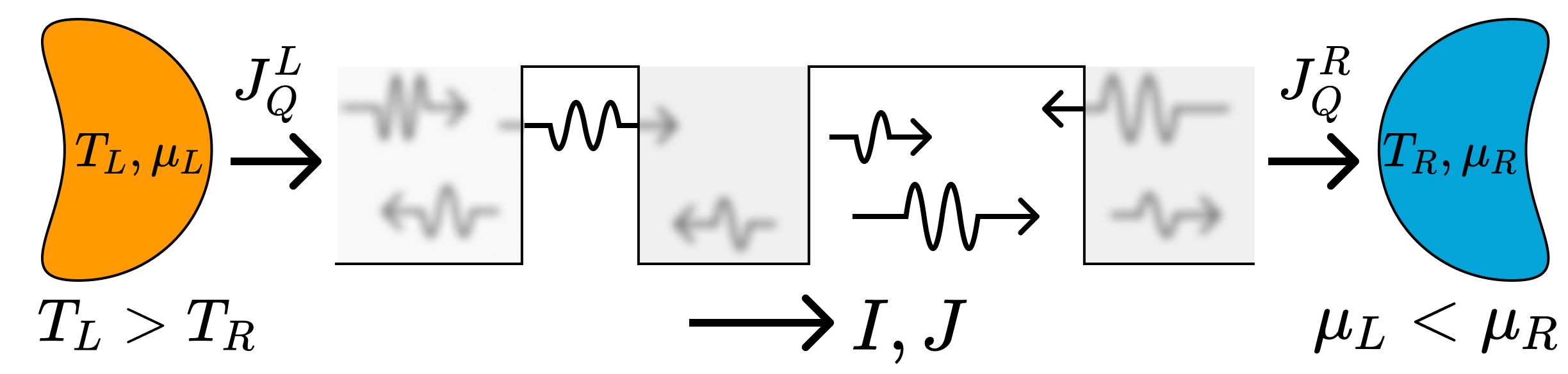
Figure 1: The transport properties across a thermoelectric device is determined by a transmission function $\mathcal{T}(\epsilon)$. In this letter we determine the $\mathcal{T}(\epsilon)$ which minimizes the fluctuations (variance) in the current, for fixed average energy and particle currents.

Thermoelectrics can also be viewed as autonomous thermal engines. The output power, associated to chemical work, is $P=-\delta_{\mu}I$, where $\delta_{\mu}=\mu_{L}-\mu_{R}$, while the heat current to each bath is given by $J_{Q}^{i}=J-\mu_{i}I$ (Fig. 1). For concreteness, we assume always $T_{L}>T_{R}$. The system will then operate as an engine when $P,J_{Q}^{L},J_{Q}^{R}>0$, in which case the efficiency is $\eta=P/J_{Q}^{L}$ Yamamoto and Hatano (2015). This interpretation allows us to draw a connection with the seminal results of Ref. Whitney (2014), which considered the transmission function maximizing the efficiency for a fixed output power. Fixing $P$ is tantamount to fixing $I$. Hence, maximizing $\eta=-\delta_{\mu}I/(J-\mu_{L}I)$ is equivalent to minimizing $J$. The problem in Whitney (2014) can thus be rephrased as which transmission function minimizes $J$ for fixed $I$.

A crucial difference with respect to our case, however, is that $\Delta_{I}^{2}$ is a non-linear (quadratic) functional of $\mathcal{T}$. Moreover, it is also a concave one. Standard tools, such as Lagrange multipliers, therefore do not apply. Intuitively speaking, the minimum of a concave function, defined on an interval, is at the boundary of said interval, not somewhere in the middle, as in the convex case. A similar argument can be made to the problem at hand, but involving a functional of $\mathcal{T}(\epsilon)$, which can be viewed as a function defined on an infinite dimensional space.

Main results– The main result of this Letter can be condensed into the following theorem (see the Supplemental Material Sup for the rigorous proof):

Theorem 1: The transmission function $\mathcal{T}(\epsilon)$ which minimizes $\Delta_{I}^{2}$ [Eq. (3)] for any number of linear constraints is a collection of boxcars, with $\mathcal{T}(\epsilon)$ being either 0 or 1; that is,

$$\mathcal{T}_{\rm opt}(\epsilon)=\sum\limits_{i}\theta(\epsilon-a_{i})\theta(b_{i}-\epsilon),$$ (4)

where $\theta(x)$ is the Heaviside function and $a_{i},b_{i}\in[-\infty,+\infty]$ are the boxcars boundary points, that are fixed by the linear constraints.

The proof holds true for an arbitrary number of linear constraints. The fact that the optimal $\mathcal{T}(\epsilon)$ is either 0 or 1 implies we can substitute $\mathcal{T}^{2}=\mathcal{T}$ in Eq. (3), and express it as $\Delta_{I}^{2}=\sum_{i}\int_{a_{i}}^{b_{i}}d\epsilon~{}g(\epsilon)$, where $g(\epsilon)=f_{L}(1-f_{L})+f_{R}(1-f_{R})$. The remaining problem may now be solved using standard Lagrange-Karush-Kuhn-Tucker multipliers Gass (1985); Boyd and Vandenberghe (2004) to locate the points $a_{i},b_{i}$. From now on, we focus on the particular case where $I$ and $J$ are fixed. This leads to our second main result Sup :

Theorem 2: The position of the optimal boxcars is determined by the regions in energy for which

$$g(\epsilon)\leqslant(\lambda\epsilon+\eta)\Delta f(\epsilon),$$ (5)

where $\lambda$ and $\eta$ are the Lagrange multipliers introduced to fix $I$ and $J$.

Since the problem is framed in terms of Lagrange multipliers, one should interpret $I(\eta,\lambda)$ and $J(\eta,\lambda)$ as functions of $\eta,\lambda$. A given choice of $\eta,\lambda$ fixes the optimal boxcar, which in turn fixes $I$ and $J$. In practice, of course, what we want is to work with fixed $I,J$, which thus requires determining the inverse functions $\eta(I,J)$ and $\lambda(I,J)$. This has to be done numerically. We developed a Python library for doing so, which can be downloaded at pyt . The calculations are facilitated by the fact that, as we show in Sup , $I$ is monotonic in $\eta$, and $J$ in $\lambda$. Once the optimal boxcar is determined for a given $I,J$, the minimal variance $\Delta_{I,{\rm opt}}^{2}$ is computed from Eq. (3), with $\mathcal{T}=\mathcal{T}_{\rm opt}$. Since the latter is by construction the smallest possible variance out of all transmission functions, it follows that $\Delta_{I}^{2}\geqslant\Delta_{I,{\rm opt}}^{2}$ for any other model. This therefore represents a generalized TUR bound. And, in addition, also establishes which process saturates it.

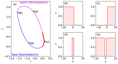
Figure 2: (a) When $(T_{L},T_{R},\mu_{L},\mu_{R})=(1,0.2,-1,1/2)$, the allowed values of $I$ and $J$, for any possible transmission function, must lie within the region formed by the curves $J_{\rm min}(I)$ and $J_{\rm max}(I)$, with $I\in[I_{\rm min},I_{\rm max}]$. The thick red part of the curve denotes the region where the system operates as an engine ($P=-\delta_{\mu}I>0$ and $J_{Q}^{L}=J-\mu_{L}I>0$). (b)-(e) Examples of boxcars at different points along the boundary. (b) $I_{\rm min}$, (c) $I_{\rm max}$, (d) $J_{\rm min}(I)$ (e) $J_{\rm max}(I)$.

Limiting cases- For each parameters set $(T_{L},T_{R},\mu_{L},\mu_{R})$, the currents $I$ and $J$ in Eq. (2) can only take values within a finite interval, irrespective of what the transmission function is. An example is shown in Fig. 2(a). Before studying the predictions of Theorems 1 and 2, it is thus convenient to establish the boundaries of this region, and then study the corresponding boxcars within them.

The particle current $I$ is bounded by two values, $I_{\rm min}$ and $I_{\rm max}$, which can be found directly from Eq. (2) by noting that $\Delta f(\epsilon)$ changes sign only once, at the point $\epsilon_{0}=\delta_{\beta\mu}/\delta_{\beta}$. Hence, $I_{\rm min/max}$ will have optimal transmission functions $\mathcal{T}(\epsilon)$ given by boxcars starting at $\epsilon_{0}$ and extending to either $\pm\infty$, respectively. These are illustrated in Figs. 2(b) and (c).

For a given $I\in[I_{\rm min},I_{\rm max}]$, the energy current $J$ will in turn be bounded by extremal values $J_{\rm min}(I)$ and $J_{\rm max}(I)$. At these lines, the solutions of Eq. (5), which minimize $\Delta_{I}^{2}$, therefore also extremize $J$. Since $I,J$, are monotonic in $\eta,\lambda$, the extrema $J_{\rm min}(I)$ and $J_{\rm max}(I)$ must occur for $\eta,\lambda\to\pm\infty$. Due to the lhs of Eq. (5) being always non-negative and finite, in this limit the condition reduces to $(\lambda\epsilon+\eta)\Delta f(\epsilon)\geqslant 0$. This expression changes sign twice, at $\epsilon_{0}$ and $\epsilon_{1}=-\eta/\lambda$ (the actual value of $\epsilon_{1}$ can be determined implicitly as a function of $I$). The curve $J_{\rm min}(I)$ corresponds to a compact boxcar in the interval $[\epsilon_{0},\epsilon_{1}]$, as illustrated in Fig. 2(d). This is precisely the “best thermoelectric” (or “most efficient”) in Ref. Whitney (2014). Conversely, the curve $J_{\rm max}(I)$ (which is the “worst thermoelectric”) is associated with the complementary boxcar, i.e. one which is 0 in $[\epsilon_{0},\epsilon_{1}]$ and 1 otherwise (Fig. 2(e)). Interestingly, we therefore see that our results also encompass those of Whitney (2014) as a particular case. However, we call attention to that fact that along these boundaries the system will not necessarily be operating as an engine. It will only do so in the region highlighted by a red thick line in Fig. 2(a).

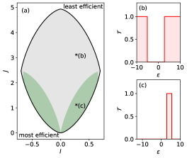
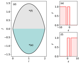
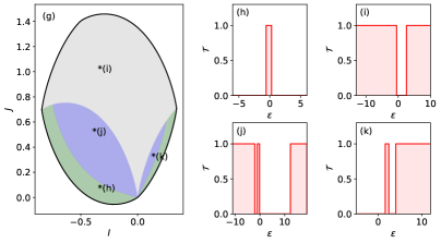
Figure 3: Examples of possible boxcar configurations. The large plots represent the allowed value of $I$ and $J$ for different sets $(T_{L},T_{R},\mu_{L},\mu_{R})$, with the colors separating regions where the boxcars are topologically different (see text). The small plots are examples of optimal boxcars in different regions. (a)-(c) $(T_{L},T_{R},\mu_{L},\mu_{R})=(2,1,0,0)$. (d)-(f) $(1,1,-1,1)$ (g)-(k) $(1,0.2,0.1,0.6)$.

Numerical examples- For values of $I,J$ inside the region defined by $J_{\rm min/max}(I)$, the shape of the boxcar must be determined numerically from Eq. (5). Due to the intricate dependence on $(T_{L},T_{R},\mu_{L},\mu_{R})$, this may result in complex boxcar shapes. Several examples are shown in Fig. 3: (a)-(c) corresponds to $\mu_{L}=\mu_{R}$; (d)-(f) to $T_{L}=T_{R}$; and (g)-(k) to a bias in both affinities. It is also possible to determine regions in the $I-J$ plane where the boxcar topology changes, represented by colored regions in Figs. 3(a),(d),(g). The boundary between these regions correspond to those values of $\lambda,\eta$ where the number of roots of $g-(\lambda\epsilon+\eta)\Delta f$ changes (see Sup for details). The largest number of boxcars we have been able to find is 3, as in Fig. 3(j). This is related to the type of constraints we are imposing. If the variance of some other current is studied, or if additional linear constraints are imposed (e.g. in the case of spin-dependent transport channels), more complex boxcars can in principle occur.

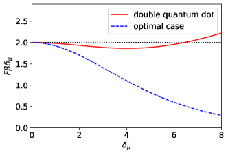
Figure 4: Red-solid: Fano factor $F=\Delta_{I}^{2}/I$, in units of $(\beta\delta_{\mu})^{-1}$, for the double quantum-dot in Eq. (6), as a function of $\delta_{\mu}$. Violations of the TUR (1) occur when this falls below 2 Ptaszyński (2018). Blue-dashed: Fano factor for the minimal variance process, computed using our framework. Parameters: $\Gamma=0.1$, $\Omega=0.05$, $\omega=0$, $\beta_{L}=\beta_{R}=1$ and $\mu_{R}=-\mu_{L}=\delta_{\mu}/2$.

Physical models- Our framework yields the transmission function with the smallest variance, for a fixed $I$ and $J$. In the examples in Figs. 2 and 3, we have chosen $I,J$ arbitrarily, by selecting points within the physically allowed region. In practice, however, one is often more interested in situations where $I$ and $J$ stem from a concrete physical model. That is, they are determined from Eq. (2) by some given transmission function $\mathcal{T}(\epsilon)$. One may then ask how does the variance associated to this transmission function fare with respect to the optimal one (obtained from Theorems 1 and 2)?

To illustrate this idea, we consider the problem studied in Ref. Ptaszyński (2018), which discussed violations of the TUR (1) in the case of a resonant double quantum-dot system, characterized by the transmission function

$$\mathcal{T}_{d}(\epsilon)=\frac{\Gamma^{2}\Omega^{2}}{|(\epsilon-\omega+i\Gamma/2)^{2}-\Omega^{2}|^{2}},$$ (6)

where $\Gamma$ is the system-bath coupling strength, $\omega$ is the excitation frequency of each dot and $\Omega$ the inter-dot hopping constant. For simplicity, we fix $T_{L}=T_{R}$ and $\mu_{R}=-\mu_{L}=\delta_{\mu}/2$.

TUR violations can be quantified by analyzing the Fano factor $F=\Delta_{I}^{2}/|I|$. Since $\sigma=\beta\delta_{\mu}I$ in this case, we see that the TUR (1) would correspond to $F\geqslant 2/(\beta\delta_{\mu})$. Violations thus occur when $F\beta\delta_{\mu}<2$. Results for the double quantum dot are shown in Fig. 4, in red-solid lines, as a function of $\delta_{\mu}$. The violations are generally small, of at most $1.86$ in this case. This, of course, depends on the choices of parameters, but other results reported in the literature are roughly of the same magnitude Saryal et al. (2021); Ptaszyński (2018); Agarwalla and Segal (2018a); Liu and Segal (2019); Saryal et al. (2019); Ehrlich and Schaller (2021). In contrast, the blue-dashed line represents the Fano factor obtained from Eq. (5). This corresponds to the same values of $I,J$ (and $\sigma$) as the red curve, but with the smallest possible $\Delta_{I,{\rm opt}}^{2}$ allowed over all transmission functions. As can be seen, $F\beta\delta_{\mu}$ is now monotonically decreasing with $\delta_{\mu}$, and tends to zero at infinite bias. Consequently, far from linear response, arbitrary violations of the TUR are possible. Conversely, close to $\delta_{\mu}\sim 0$, one recovers $F\beta\delta_{\mu}=2$.

Since $\beta_{L}=\beta_{R}=\beta$ and $\mu_{R}=-\mu_{L}=\delta_{\mu}/2$, this scenario is located exactly at the boundary between the gray and cyan curves in Fig. 3(d). The optimal transmission function is found to be a single boxcar of the form $[-a/2,a/2]$ . For boxcars of this form, it is actually possible to determine the optimal Fano factor $F_{\rm opt}=\Delta_{I,{\rm opt}}^{2}/|I|$ analytically, by directly computing the integrals in Eqs. (2) and (3). The result is $F_{\rm opt}=2(1-f_{L}-f_{R})/[\ln f_{R}(1-f_{R})f_{L}(1-f_{L})]$, where $f_{L(R)}=f_{L(R)}(a/2)$ are the Fermi-Dirac functions of each bath, evaluated at the right-end of the boxcar.

Linear regime- The results above illustrate that, far from linear response, it is impossible to bound $\Delta_{I}^{2}$ in terms only of $I$ and $\sigma$. In fact, our results just showed that far from linear response, arbitrary violations of the TUR are possible (similarly to what was found in Ehrlich and Schaller (2021)). Conversely, one may naturally ask whether the situation simplifies in the linear regime. We parametrize $\beta_{L}=\beta-\delta_{\beta}/2$, $\beta_{R}=\beta+\delta_{\beta}/2$, and $\beta_{L}\mu_{L}=\beta\mu-\delta_{\beta\mu}/2$, $\beta_{R}\mu_{R}=\beta\mu+\delta_{\beta\mu}/2$. Using this in both sides of Eq. (5) yields $g(\epsilon)\simeq 2f(1-f)$ and $\Delta f\simeq(\delta_{\beta}\epsilon-\delta_{\beta\mu})f(1-f)$, where $f=(e^{\beta(\epsilon-\mu)}+1)^{-1}$ is the Fermi-Dirac distribution associated to the mean temperature and chemical potential. Hence, the position of the boxcars is now determined by $2\leqslant(\lambda\epsilon+\eta)(\delta_{\beta}\epsilon-\delta_{\beta\mu})$, which is a quadratic equation. The optimal transmission function must therefore be either a single boxcar, in an interval $[a,b]$ (as in Fig. 2(d)), or two boxcars in $(-\infty,a]$ and $[b,\infty)$ (as in Fig. 2(e)). The actual values of $a$ and $b$ are determined by fixing $I$ and $J$.

To determine the behavior of the TUR in the linear regime, we expand Eq. (2) in powers of $\delta_{\beta}$ and $\delta_{\beta\mu}$. This allows us to write $I=\delta_{\beta}\theta_{1}-\delta_{\beta\mu}\theta_{0}$ and $J=\delta_{\beta}\theta_{2}-\delta_{\beta\mu}\theta_{1}$, where $\theta_{n}=\int_{B}d\epsilon~{}\epsilon^{n}f(1-f)$, and $B$ denotes the boxcar in question. The variance (3), on the other hand, becomes $\Delta_{I}^{2}=2\theta_{0}$. Combining this with $\sigma=-\delta_{\beta}J+\delta_{\beta\mu}I$ then yields

$$\frac{\Delta_{I}^{2}\sigma}{I^{2}}=2+\frac{2\delta_{\beta}^{2}}{I^{2}}(\theta_{0}\theta_{2}-\theta_{1}^{2}).$$ (7)

This result actually holds for any boxcar; the only assumption is linear response. If $\delta_{\beta}=0$, as in Fig. 4, then the linear response limit is exactly $2$, which is the TUR (1). Conversely, if $\delta_{\beta}\neq 0$, using Jensen’s inequality one may show that $\theta_{0}\theta_{2}\geqslant\theta_{1}^{2}$. Hence, the rhs of (7) will be strictly larger than 2. This means that, at linear response the TUR (1) does indeed hold; however, it is generally loose, unless $\delta_{\beta}=0$.

Discussion. In this paper we have provided a definitive answer to the question of TUR violations in quantum thermoelectrics. We showed that, beyond linear response, no bound exists which relate $\Delta_{I}^{2}$ only to $I$ and $\sigma$; instead, the trade-off relation involving these quantities becomes dependent on the system parameters. Our approach addresses this issue by determining what is the optimal process; i.e., out of all possible processes allowed in Nature, which one yields the smallest possible variance for a fixed $I$ and $\sigma$? We believe this represents a very insightful question. First, it yields more general bounds, not necessarily related only to $I$ and $\sigma$. And second, and most importantly, it actually tells us which process is the optimal one.

Recently, there has been growing interest in this kind of approach. Irrespective of whether or not achieving the optimal process is easy, knowing what it is provides a benchmark which must be satisfied by any other process. For instance, Ref. Cavina et al. (2016) determined the probability distribution maximizing work extraction in the single shot-scenario. This was later studied experimentally in Maillet et al. (2019), which performed a process that was not exactly optimal, but got extremely close.

The design of transmission functions in quantum thermoelectrics is a relevant technological problem. Our results introduce fluctuations as a new ingredient to the mix. It provides, to our knowledge, the only known route for designing transmission functions with target power and efficiency, but also minimizing fluctuations.

Acknowledgements– GTL acknowledges the financial support of the São Paulo Funding Agency FAPESP (Grants No. 2017/50304-7, 2017/07973-5 and 2018/12813-0), the Gridanian Research Council (GRC), and the Brazilian funding agency CNPq (Grant No. INCT-IQ 246569/2014-0). G. G. acknowledges support from FQXi and DFG FOR2724 and also from the European Union Horizon 2020 research and innovation programme under the Marie Sklodowska-Curie grant agreement No. 101026667.

This supplemental material contains the rigorous proof of Theorems 1 and 2 of the main text. The problem consists in minimizing the variance $\Delta_{I}^{2}$ [Eq. (3)] subject to a set of linear (in $\mathcal{T}$) constraints; in our case, fixed $I$ and $J$. Formally, this may be written as the following mathematical optimization problem:

$$\mbox{Minimize }\int_{-\infty}^{\infty}f(x)\beta(x)-f(x)^{2}\gamma(x)^{2}\mathrm{d}x\quad\mbox{subject to}$$

$$\int_{-\infty}^{\infty}f(x)\alpha_{i}(x)\mathrm{d}x=\phi_{i},\,\,\,i=1,\ldots,n\quad\mbox{and}\quad 0\leq f(x)\leq 1\,\,\forall\,\,x\in\mathds{R}$$ (S1)

This is a concave functional of $f(x)$, which therefore requires specific methods in order to be tackled.

In what follows, we start by fixing the necessary notations and definitions employed throughout this Supplementary Material. The proofs of Theorems 1 and 2 are then given in Secs. II and III, respectively. A series of additional remarks and details are finally provided in Sec. IV.

I Notations, Definitions and Standing Hypotheses

To make things precise, we make the following hypothesis and definitions:

• We will denote by $\widetilde{\mathcal{R}}$ the set of functions $f:\mathds{R}\rightarrow\mathds{R}$ that are bounded and such that for every compact interval $[a,b]$, $f$ has only finitely many discontinuities in $[a,b]$. Furthermore, we will denote by $\mathcal{R}$ the subset of $\widetilde{\mathcal{R}}$ where $\mathrm{Im}(f)\subseteq[0,1]$.

• $\alpha_{i}$, $\beta$ and $\gamma$ will always denote functions in $\widetilde{\mathcal{R}}$, such that

  $$\int_{-\infty}^{\infty}|\alpha_{i}(x)|\mathrm{d}x,\quad\int_{-\infty}^{\infty}|\beta(x)|\mathrm{d}x\quad\mbox{and}\quad\int_{-\infty}^{\infty}\gamma(x)^{2}\mathrm{d}x$$

  are all finite and such that $\alpha_{i}(x)\neq 0$, $\beta(x)\neq 0$ and $\gamma(x)\neq 0$ almost everywhere.

• We define the following functionals acting on functions in $\mathcal{R}$:

  $$\mathcal{C}_{i}[f]=\int_{-\infty}^{\infty}f(x)\alpha_{i}(x)\mathrm{d}x,\quad i=1,\ldots,n\quad\quad\quad\quad\quad\quad\mathcal{Q}[f]=\int_{-\infty}^{\infty}f(x)\beta(x)-f(x)^{2}\gamma(x)^{2}\mathrm{d}x$$

  $$\mathcal{L}[f]=\int_{-\infty}^{\infty}f(x)(\beta(x)-\gamma(x)^{2})\mathrm{d}x\quad\quad\quad\mbox{and}\quad\quad\quad\mathcal{B}[f]=\int_{-\infty}^{\infty}\gamma(x)^{2}f(x)(1-f(x))\mathrm{d}x$$

  The functionals $\mathcal{C}_{i}$ are the ones that give us the constraints in (S1), while $\mathcal{Q}$ is the one to be optimized. As we will see further on, the functional $\mathcal{L}$ can be regarded as a linearized version of $\mathcal{Q}$. Finally, $\mathcal{B}[f]$ can be used as a measure of how far $f$ is from being a boxcar.

• We will be using the following jargon from optimization theory Gass (1985); Boyd and Vandenberghe (2004):

  • A feasible point (function) of an optimization problem is a point (function) that obeys all the constraints.

  • The feasible region is the set of all feasible points (functions).

  • The optimal value is the value of the desired extremum.

  • An optimal point (function) is a feasible point (function) that attains the desired extremum.

• The feasible region for the problem (S1) will be denoted $\mathcal{F}$:

  $$\mathcal{F}=\left\{f\in\mathcal{R}\mbox{ such that }\mathcal{C}_{i}[f]=\phi_{i}\,\forall\,i\right\},$$

• We will denote by $\mathsf{Q}$ and $\mathsf{L}$ the optimal values minimizing $\mathcal{Q}$ and $\mathcal{L}$ respectively, given the constraints $\mathcal{C}_{i}$:

  $$\mathsf{Q}=\inf_{f\in\mathcal{F}}\mathcal{Q}[f]\quad\quad\mbox{and}\quad\quad\mathsf{L}=\inf_{f\in\mathcal{F}}\mathcal{L}[f]$$

  Note that the hypothesis made about $\beta$ and $\gamma$ imply that $\mathsf{Q}$ and $\mathsf{L}$ must be finite when $\mathcal{F}\neq\varnothing$.

• We will denote by $\mathcal{D}(F)$ the set of discontinuities of a function $F:\mathds{R}\rightarrow\mathds{R}$

• Finally, we recall the definition of oscillation of a function $f$ in an interval (as used in Analysis):

  $$\omega_{f}(I)=\sup_{x\in I}f(x)-\inf_{x\in I}f(x)$$

II Proof of theorem 1

We start by proving theorem 1, namely

Theorem 1.

The transmission function $\mathcal{T}(\epsilon)$ which minimizes $\Delta_{I}^{2}$ [Eq. (3)] for any number of linear constraints is a collection of boxcars, with $\mathcal{T}(\epsilon)$ being either 0 or 1; that is,

$$\mathcal{T}_{\rm opt}(\epsilon)=\sum\limits_{i}\theta(\epsilon-a_{i})\theta(b_{i}-\epsilon),$$

where $\theta(x)$ is the Heaviside function and $a_{i},b_{i}\in[-\infty,+\infty]$ are the boxcars boundary points that are fixed by the linear constraints in question.

This will actually be accomplished by proving the following statement (using the notations we just defined):

If $$f\in\mathcal{F} \mathcal{Q}[f]\leq\mathsf{Q}+\delta \mathcal{B}[f]\leq\delta$$ is such that , then (S2)

Proof.

As a first step we will show that if $f\in\mathcal{F}$, then for all $\varepsilon>0$ there exist $g,h\in\mathcal{F}$ such that $\mathcal{Q}[g]\leq\mathcal{Q}[f]$, $\mathcal{L}[h]\leq\mathcal{L}[f]$ and $\mathcal{B}[g],\mathcal{B}[h]\leq\varepsilon$. To see this, let us consider $\eta>0$, an arbitrary positive number and $[a,b]$ a compact interval. Since $f\in\mathcal{R}$, then $\mathcal{D}(f)\cap[a,b]$ is finite and there exist $D$ open intervals $I_{1},\ldots,I_{D}$, all of which have measures less than $\eta$ and such that if $\mathcal{I}=\bigcup_{i}I_{i}$, then $\mathcal{D}(f)\cap[a,b]\subseteq\mathcal{I}$. As a consequence $f$ has no discontinuities on $\mathcal{J}=[a,b]\setminus\mathcal{I}$. As such, every point $x\in\mathcal{J}$ has an open interval $N_{x}$ containing it, such that the oscillation of $f$ in this interval, $\omega_{f}(N_{x})$ is less than $\eta$. Since the $N_{x}$ form an open cover of $\mathcal{J}$ and $\mathcal{J}$ is compact, then there exists a subcover that is finite: $M_{1},\ldots,M_{C}$.

Let us consider a partition $\Pi$ of the interval $[a,b]$, such that all the endpoints of the $I_{k}$ and the $M_{k}$ intervals that lie in $[a,b]$ are included and none of the subintervals has a measure larger than $\eta$. We will denote by $J_{i}$ the $N$ open subintervals of $\Pi$ such that $\omega_{f}<\eta$ and by $K_{i}$ the remaining ones. Note that the measure of the union of the $J_{i}$ must be at least $b-a-D\eta$ and hence the measure for the union of the $K_{i}$ is at most $D\eta$.

We then define the constants

$$f^{(-)}_{i}=\inf_{x\in J_{i}}f(x),\quad\quad f^{(+)}_{i}=\sup_{x\in J_{i}}f(x),\quad\quad\mbox{and}\quad\quad m_{i}=1-f^{(+)}_{i}+f^{(-)}_{i}$$

the integrals

$$a_{i,j}=\int_{J_{j}}\alpha_{i}(x)\mathrm{d}x,\quad\quad\quad\quad\quad\quad b_{j}=-\int_{J_{j}}f^{(-)}_{j}(\beta(x)+(f^{(-)}_{j}-2f(x))\gamma(x)^{2})\mathrm{d}x,$$

$$c_{j}=m_{j}\int_{J_{j}}(\beta(x)+2(f^{(-)}_{j}-f(x))\gamma(x)^{2})\mathrm{d}x,\quad\quad\quad\quad\quad\quad d_{j}=m_{j}^{2}\int_{J_{j}}\gamma(x)^{2}\mathrm{d}x,$$

$$b^{\prime}_{j}=-\int_{J_{j}}f^{(-)}_{j}(\beta(x)-\gamma(x)^{2})\mathrm{d}x,\quad\quad\quad\quad\quad\quad c^{\prime}_{j}=m_{j}\int_{J_{j}}(\beta(x)-\gamma(x)^{2})\mathrm{d}x$$

and the functions

$$F_{\lambda}(x)=\left\{\begin{array}[]{ll}f(x)-f^{(-)}_{i}+m_{i}\lambda_{i}&\mbox{if }x\in J_{i}\\ f(x)&\mbox{otherwise}\end{array}\right.$$

It follows that if $0\leq\lambda_{i}\leq 1$, then $F_{\lambda}\in\mathcal{R}$ and we also have

$$\mathcal{C}_{i}[F_{\lambda}]=\phi_{i}+\sum_{j}a_{i,j}(m_{j}\lambda_{j}-f^{(-)}_{j}),\quad\quad\quad\quad\quad\quad\mathcal{Q}[F_{\lambda}]=\mathcal{Q}[f]+\sum_{j}(b_{j}+c_{j}\lambda_{j}-d_{j}\lambda_{j}^{2})\quad\quad\mbox{and}$$

$$\mathcal{L}[F_{\lambda}]=\mathcal{L}[f]+\sum_{j}(b^{\prime}_{j}+c^{\prime}_{j}\lambda_{j}).$$

Furthermore, if $\mu_{i}=\nicefrac{{f^{(-)}_{i}}}{{m_{i}}}$ for every $i$ such that $m_{i}\neq 0$ ($\mu_{i}$ can be any value in $[0,1]$ if $m_{i}=0$), then we have $F_{\mu}=f$. Consider then the following concave programming problems:

Minimize

$$\sum_{j}(b_{j}+c_{j}\lambda_{j}-d_{j}\lambda_{j}^{2})\mbox{ subject to the constraints}$$

$$\sum_{j}a_{i,j}(m_{j}\lambda_{j}-f^{(-)}_{j})=0\quad\quad\mbox{and}\quad\quad 0\leq\lambda_{i}\leq 1\,\forall\,i$$ (S3)

and

Minimize

$$\sum_{j}(b^{\prime}_{j}+c^{\prime}_{j}\lambda_{j})\mbox{ subject to the constraints}$$

$$\sum_{j}a_{i,j}(m_{j}\lambda_{j}-f^{(-)}_{j})=0\quad\quad\mbox{and}\quad\quad 0\leq\lambda_{i}\leq 1\,\forall\,i$$ (S4)

Since $F_{\mu}=f$, then $(\mu_{1},\ldots,\mu_{N})$ is a feasible point for both (S3) and (S4) corresponding in both cases to a value 0 for the objective function. As a consequence, if $\nu=(\nu_{1},\ldots,\nu_{N})$ and $\sigma=(\sigma_{1},\ldots,\sigma_{N})$ are optimal points for (S3) and (S4) respectively, it follows that $\mathcal{C}_{i}[F_{\nu}]=\mathcal{C}_{i}[F_{\sigma}]=\phi_{i}$, while $\mathcal{Q}[F_{\nu}]\leq\mathcal{Q}[f]$ and $\mathcal{L}[F_{\sigma}]\leq\mathcal{L}[f]$. So we need to show that we can choose $\eta$ and $[a,b]$ in such a way that $\mathcal{B}[F_{\nu}],\mathcal{B}[F_{\sigma}]\leq\varepsilon$. In what follows $\xi$ means either $\nu$ or $\sigma$ (the argument is identical). To see why we can make $\mathcal{B}[F_{\xi}]\leq\varepsilon$, note that in both cases the feasible region $R$ will be the intersection of a hypercube $[0,1]^{N}$ and $n$ hyperplanes defining the linear constraints. Since there is always an extremal point of the feasible region where the optimum of a concave problem is attained Horst and Tuy (1993), then one needs only to look for the extremal points of $R$. Since $R$ is a polytope, the extremal points are the vertexes, which in this case are all points where at least $N-n$ coordinates are either 0 or 1, implying that $\xi$ has at least $N-n$ coordinates that are either 0 or 1. In turn, this implies that

• If $x\in J_{i}$ and $\xi_{i}=0$, then $0\leq F_{\xi}\leq\eta$

• If $x\in J_{i}$ and $\xi_{i}=1$, then $1-\eta\leq F_{\xi}\leq 1$

• If $x\in J_{i}$ but $\xi_{i}\neq 0,1$, then we can only say $0\leq F_{\xi}\leq 1$

Assuming $\eta<\nicefrac{{1}}{{2}}$, it follows that

$$\mathcal{B}[F_{\xi}]=\int_{-\infty}^{\infty}\gamma(x)^{2}F_{\xi}(x)(1-F_{\xi}(x))\mathrm{d}x=\underbrace{\int_{-\infty}^{a}\ldots+\int_{b}^{\infty}\ldots}_{\mathcal{B}_{1}}+\underbrace{\sum_{i}\int_{K_{i}}\ldots}_{\mathcal{B}_{2}}+\underbrace{\sum_{j}\int_{J_{j}}\ldots}_{\mathcal{B}_{3}}$$

where we simply broke the integral over different intervals. Since the integral $\int_{-\infty}^{\infty}\gamma(x)^{2}\mathrm{d}x$ is finite (from our hypotheses) and $0\leq F_{\xi}(x)(1-F_{\xi}(x))\leq 1$, then it is trivial that we can choose $[a,b]$ such that $\mathcal{B}_{1}\leq\nicefrac{{\varepsilon}}{{3}}$ by choosing a sufficiently large interval. Since the measure of $\bigcup_{i}K_{i}$ is at most $D\eta$ and $\gamma(x)^{2}$ is bounded (again from our hypotheses), then one can easily bound $\mathcal{B}_{2}$:

$$\mathcal{B}_{2}=\sum_{i}\int_{K_{i}}\gamma(x)^{2}F_{\xi}(x)(1-F_{\xi}(x))\mathrm{d}x\leq\sum_{i}\int_{K_{i}}\Gamma\mathrm{d}x\leq D\eta\Gamma$$

where $\Gamma$ is any upper bound for $\gamma(x)^{2}$. So we can take $\mathcal{B}_{2}\leq\nicefrac{{\varepsilon}}{{3}}$ by choosing a sufficiently small $\eta$ (namely $\eta\leq\nicefrac{{\varepsilon}}{{3D\Gamma}}$). Finally, $\mathcal{B}_{3}$ can be bounded in a similar way, because if $\eta<\nicefrac{{1}}{{2}}$ and $x\in J_{i}$ (where $\xi_{i}=0$ or 1), then $F_{\xi}(x)(1-F_{\xi}(x))\leq\eta(1-\eta)\leq\eta$. Furthermore, the measure of the $J_{i}$ intervals where $\xi_{i}\neq 0,1$ is at most $n\eta$. So:

$$\mathcal{B}_{3}=\sum_{j}\int_{J_{j}}\gamma(x)^{2}F_{\xi}(x)(1-F_{\xi}(x))\mathrm{d}x=\!\!\sum_{\begin{subarray}{c}j\\ \xi_{j}=0\text{ or }1\end{subarray}}\int_{J_{j}}\gamma(x)^{2}F_{\xi}(x)(1-F_{\xi}(x))\mathrm{d}x+\!\!\sum_{\begin{subarray}{c}j\\ \xi_{j}\neq 0,1\end{subarray}}\int_{J_{j}}\gamma(x)^{2}F_{\xi}(x)(1-F_{\xi}(x))\mathrm{d}x\leq$$

$$\leq\sum_{\begin{subarray}{c}j\\ \xi_{j}=0\text{ or }1\end{subarray}}\int_{J_{j}}\Gamma\eta\mathrm{d}x+\!\!\sum_{\begin{subarray}{c}j\\ \xi_{j}\neq 0,1\end{subarray}}\int_{J_{j}}\Gamma\mathrm{d}x\leq\Gamma\eta\left(b-a+n\right)$$

So we can take $\mathcal{B}_{3}\leq\nicefrac{{\varepsilon}}{{3}}$ by making $\eta$ sufficiently small ($\eta\leq\nicefrac{{\varepsilon}}{{3\Gamma(b-a+n)}}$). It follows that by taking $[a,b]$ large enough and $\eta\leq\min\left\{\nicefrac{{1}}{{2}},\nicefrac{{\varepsilon}}{{3D\Gamma}},\nicefrac{{\varepsilon}}{{3\Gamma(b-a+n)}}\right\}$ we get $\mathcal{B}[F_{\xi}]\leq\varepsilon$ (so $g=F_{\nu}$ and $h=F_{\sigma}$)

The second step in the proof is that this implies that $\mathsf{Q}=\mathsf{L}$. Let $\delta,\varepsilon>0$ and let $u\in\mathcal{F}$ be such that $\mathcal{L}[u]\leq\mathsf{L}+\delta$. By what we just proved, there exists $U\in\mathcal{F}$ such that $\mathcal{L}[U]\leq\mathcal{L}[u]\leq\mathsf{L}+\delta$ and $\mathcal{B}[U]\leq\varepsilon$. We now call attention to the fact that $\mathcal{Q}=\mathcal{L}+\mathcal{B}$, so we have

$$\mathsf{Q}\leq\mathcal{Q}[U]=\mathcal{L}[U]+\mathcal{B}[U]\leq\mathsf{L}+\delta+\varepsilon$$

Since this is true for any $\delta,\varepsilon>0$ it implies $\mathsf{Q}\leq\mathsf{L}$. On the other hand, if $v\in\mathcal{F}$ is such that $\mathcal{Q}[v]\leq\mathsf{Q}+\delta$, then there exists $V\in\mathcal{F}$ such that $\mathcal{Q}[V]\leq\mathcal{Q}[v]\leq\mathsf{Q}+\delta$ and $\mathcal{B}[V]\leq\varepsilon$. So

$$\mathsf{L}\leq\mathcal{L}[V]=\mathcal{Q}[V]-\mathcal{B}[V]\leq\mathsf{Q}+\delta$$

because $\mathcal{B}[V]\geq 0$. Once again, since this is true for any $\delta,\varepsilon>0$ it implies $\mathsf{L}\leq\mathsf{Q}$ and hence that $\mathsf{L}=\mathsf{Q}$.

This leads us to the last step of the proof. Let $\phi\in\mathcal{F}$ be such that $\mathcal{Q}[\phi]\leq\mathsf{Q}+\delta$, then we have

$$\mathcal{L}[\phi]+\mathcal{B}[\phi]\leq\mathsf{Q}+\delta\Rightarrow\mathcal{B}[\phi]\leq\delta+\mathsf{Q}-\mathcal{L}[\phi]=\delta+\mathsf{L}-\mathcal{L}[\phi]\leq\delta$$

∎

What we proved here is an actual proof of the statement in the main text, because it means that as we consider transmission functions that are closer and closer to being optimal ($\mathcal{Q}[\mathcal{T}]\rightarrow\mathsf{Q}$) we will be taking $\delta\rightarrow 0$ and hence these transmission functions are getting closer and closer to being a boxcar ($\mathcal{B}[\mathcal{T}]\rightarrow 0$). In particular, if $\mathcal{T}$ is an optimal function, then $\mathcal{Q}[\mathcal{T}]=\mathsf{Q}$ implying that $\mathcal{Q}[\mathcal{T}]\leq\mathsf{Q}+\delta$ for all $\delta\geq 0$, so $\mathcal{B}[\mathcal{T}]\leq\delta$ in this case would imply that $\mathcal{B}[\mathcal{T}]=0$ and hence that $\mathcal{T}$ is a boxcar almost everywhere.

III Proof of theorem 2

We now move our attention to the second theorem stated in the main text, namely

Theorem 2.

The position of the optimal boxcars is determined by the regions in energy for which

$$g(\epsilon)\leqslant(\lambda\epsilon+\eta)\Delta f(\epsilon),$$

where $\lambda$ and $\eta$ are Lagrange multipliers introduced to fix $I$ and $J$.

Proof.

Using theorem 1, it follows from Eqs. (2) and (3) of the main text that, for a transmission function $\mathcal{T}$ that is optimal we must have

$$I(a_{1},b_{1},\ldots,b_{N})=\sum_{i}\int_{a_{i}}^{b_{i}}\Delta f(\epsilon)d\epsilon,\quad\quad J(a_{1},b_{1},\ldots,b_{N})=\sum_{i}\int_{a_{i}}^{b_{i}}\Delta f(\epsilon)\epsilon d\epsilon\quad\quad\mbox{and}$$

$$\Delta^{2}_{I,\mathrm{opt}}(a_{1},b_{1},\ldots,b_{N})=\sum_{i}\int_{a_{i}}^{b_{i}}g(\epsilon)d\epsilon,$$

where, recall, $\Delta f(\epsilon)=f_{L}(\epsilon)-f_{R}(\epsilon)$ and $g(\epsilon)=f_{L}(1-f_{L})+f_{R}(1-f_{R})$. So if we consider a Lagrangian $L(a_{1},b_{1},\ldots,b_{N};\lambda,\eta)=\Delta^{2}_{I,\mathrm{opt}}+\lambda(J-J_{0})+\eta(I-I_{0})$, then the extrema are solutions of the system

$$\left\{\begin{array}[]{l}g(a_{i})=(\lambda a_{i}+\eta)\Delta f(a_{i})\\ g(b_{i})=(\lambda b_{i}+\eta)\Delta f(b_{i})\\ I(a_{1},b_{1},\ldots,b_{N})=I_{0}\\ J(a_{1},b_{1},\ldots,b_{N})=J_{0}\\ a_{1}\leq b_{1}\leq a_{2}\leq b_{2}\leq\ldots\leq a_{N}\leq b_{N}\end{array}\right.$$

As such we can further determine that the endpoints of the boxcar predicted in theorem 1 obey $g(\epsilon)=(\lambda\epsilon+\eta)\Delta f(\epsilon)$. However, this still doesn’t tell us what are the intervals that constitute the actual optimal boxcar. To find this out, let us consider first the values of the multipliers ($\lambda^{*},\eta^{*}$) for which the optimal boxcar is attained and let $\Pi$ be the partition of the line created by the solutions in $\epsilon$ to $g(\epsilon)=(\lambda^{*}\epsilon+\eta^{*})\Delta f(\epsilon)$. Exploring the fact that $\mathsf{Q}=\mathsf{L}$ (as seen in the proof for theorem 1), we can then consider the problem of minimizing $\mathcal{L}$ for a transmission function in $\mathcal{R}$ that is constant on the intervals in $\Pi$ (so that it is piecewise constant) and satisfies the constraints for $I$ and $J$. This optimization problem would read

Minimize

$$\sum_{i=1}^{N}A_{i}\tau_{i}\mbox{ subject to the constraints}$$

$$0\leq\tau_{i}\leq 1,\quad\quad\quad\sum_{i=1}^{N}B_{i}\tau_{i}=I_{0}\quad\quad\quad\mbox{and}\quad\quad\quad\sum_{i=1}^{N}C_{i}\tau_{i}=J_{0}$$ (S5)

where

$$A_{i}=\int_{\mathcal{I}_{i}}g(\epsilon)d\epsilon,\quad\quad\quad B_{i}=\int_{\mathcal{I}_{i}}\Delta f(\epsilon)d\epsilon,\quad\quad\quad C_{i}=\int_{\mathcal{I}_{i}}\epsilon\Delta f(\epsilon)d\epsilon$$

and $\mathcal{I}_{1},\ldots,\mathcal{I}_{N}$ are the intervals in $\Pi$. By construction there is an optimal solution where the $\tau_{i}$ (the value of the transmission function in $\mathcal{I}_{i}$) are either 0 or 1. Examining the Karush–Kuhn–Tucker (KKT) conditions Gass (1985); Boyd and Vandenberghe (2004) of the problem (S5) we get

$$x_{i},y_{i}\geq 0,\quad\quad x_{i}(\tau_{i}-1)=y_{i}\tau_{i}=0\quad\quad\mbox{and}\quad\quad A_{i}+(x_{i}-y_{i})-\lambda^{*}C_{i}-\eta^{*}B_{i}=0,\quad\quad\mbox{for }i=1,\ldots,N$$ (S6)

It is easy to show that a consequence of (S6) is that

$$\tau_{i}=0\Rightarrow A_{i}-\lambda^{*}C_{i}-\eta^{*}B_{i}\geq 0\quad\quad\mbox{and}\quad\quad\tau_{i}=1\Rightarrow A_{i}-\lambda^{*}C_{i}-\eta^{*}B_{i}\leq 0$$

Noticing that

$$A_{i}-\lambda^{*}C_{i}-\eta^{*}B_{i}=\int_{\mathcal{I}_{i}}g(\epsilon)-(\lambda^{*}\epsilon+\eta^{*})\Delta f(\epsilon)d\epsilon$$

and that by hypothesis $g(\epsilon)-(\lambda^{*}\epsilon+\eta^{*})\Delta f(\epsilon)$ doesn’t change signs inside of $\mathcal{I}_{i}$, this implies that the optimal boxcar (which is the one satisfying the KKT conditions) must be the one determined by:

$$g(\epsilon)-(\lambda^{*}\epsilon+\eta^{*})\Delta f(\epsilon)\leq 0$$

concluding the proof. ∎

IV Miscellaneous remarks

IV.1 General structure of the boxcars

As $\lambda$ and $\eta$ change, the boxcars they represent, change. To understand how these changes happen, we notice that they happen because the solutions for $g(x)=(\lambda x+\eta)\Delta f(x)$ change. In a sense these changes will be “continuous”. What we mean by that is that as $(\lambda,\eta)$ changes, no boxcars with lengths larger than 0 suddenly appear, nor do any boxcars change their lengths discontinuously (barring potential mergers of boxcars)

This happens because the endpoints of each boxcar can only change continuously (as a consequence of the implicit function theorem), with the exception of situations where 2 intervals merge and situations where a new interval appears (which are the situations where the hypotheses for the implicit function theorem are not satisfied for the corresponding endpoints). However, since $\mathcal{G}(x)\equiv\nicefrac{{g(x)}}{{\Delta f(x)}}$ has no open interval such that its restriction to it is affine, then even these situations can only happen with the corresponding intervals changing smoothly (for the case of a merger, the endpoints can get arbitrarily close in a continuous way while for the case of a new interval, it must always appear with its endpoints arbitrarily close and changing continuously from that point on). As a consequence, the functions $I(\lambda,\eta),J(\lambda,\eta)$ and $\Delta_{I,{\rm opt}}^{2}(\lambda,\eta)$ are continuous.

Since the points/lines $(\lambda,\eta)$ where these mergers and new intervals can occur are points where a slight perturbation can change the topology of the boxcars, we will call them bifurcations and denote their set by $\mathcal{B}$. There are actually 2 types of bifurcations:

• $(\lambda,\eta)$ is such that $g(x)-(\lambda x+\eta)\Delta f(x)$ has a double root at $z$. This happens when $\lambda=\mathcal{G}^{\prime}(z)$, $\eta=\mathcal{G}(z)-z\mathcal{G}^{\prime}(z)$.

• $\lambda=0$. This is a bifurcation because any change to $\lambda$ creates a new root (that is “coming from infinity”), as $\mathcal{G}(z)$ has finite limits when $z\rightarrow\pm\infty$

So we can write $\mathcal{B}=\mathcal{B}_{\mathrm{tan}}\cup\mathcal{B}_{0}$:

$$\mathcal{B}_{\mathrm{tan}}=\{(\mathcal{G}^{\prime}(z),\mathcal{G}(z)-z\mathcal{G}^{\prime}(z))|z\in[a,b]\setminus\{\varepsilon_{S}\}\}$$

$$\mathcal{B}_{0}=\{(0,\eta)|\eta\in\mathds{R}\}$$

If we map the curves in $\mathcal{B}$ from the plane $(\lambda,\eta)$ to $(I,J)$, we get a delimitation of different regions where the optimal boxcar configurations are topologically different.

IV.2 Derivatives and monotonicity of $I(\lambda,\eta)$ and $J(\lambda,\eta)$

When $(\lambda,\eta)\notin\mathcal{B}$, then the functions $I$ and $J$ can be differentiated via the implicit function theorem. In this case, $R(x;\lambda,\eta)\equiv g(x)-(\lambda x+\eta)\Delta f(x)$ only has simple roots. Let $x^{*}$ be such a root. Applying the implicit function theorem yields

$$\frac{\partial x^{*}}{\partial\eta}=\frac{\Delta f(x^{*})}{R^{\prime}(x^{*};\lambda,\eta)}\quad\quad\mbox{and}\quad\quad\frac{\partial x^{*}}{\partial\lambda}=\frac{x^{*}\Delta f(x^{*})}{R^{\prime}(x^{*};\lambda,\eta)}$$ (S7)

The boxcar corresponding to $(\lambda,\eta)$ is the indicator function of an union $\bigcup_{k}[a_{k},b_{k}]$, with $a_{1}<b_{1}<\ldots<a_{n}<b_{n}$ (where we can potentially have $a_{1}=-\infty$ or $b_{n}=\infty$). Define then

$$\xi_{k}=\left\{\begin{array}[]{cl}0&\mbox{if }a_{k}=-\infty\\ \frac{\Delta f(a_{k})^{2}}{R^{\prime}(a_{k};\lambda,\eta)}&\mbox{otherwise}\end{array}\right.\quad\quad\mbox{and}\quad\quad\theta_{k}=\left\{\begin{array}[]{cl}0&\mbox{if }b_{k}=\infty\\ \frac{\Delta f(b_{k})^{2}}{R^{\prime}(b_{k};\lambda,\eta)}&\mbox{otherwise}\end{array}\right.$$

Since $I$ and $J$ will be given by

$$I=\sum_{i}\int_{a_{i}}^{b_{i}}\Delta f(\epsilon)d\epsilon,\quad\quad J=\sum_{i}\int_{a_{i}}^{b_{i}}\Delta f(\epsilon)\epsilon d\epsilon$$

then from eq (S7) one obtains

$$\frac{\partial I}{\partial\eta}=\sum_{k}(\theta_{k}-\xi_{k}),\quad\quad\frac{\partial I}{\partial\lambda}=\frac{\partial J}{\partial\eta}=\sum_{k}(\theta_{k}b_{k}-\xi_{k}a_{k})\quad\quad\mbox{and}\quad\quad\frac{\partial J}{\partial\lambda}=\sum_{k}(\theta_{k}b_{k}^{2}-\xi_{k}a_{k}^{2})$$

Since $a_{k}$ is always the leftmost end of one of the boxcar pieces, then either $a_{k}=-\infty$ or $R^{\prime}(a_{k};\lambda,\eta)<0$. Similarly, since the $b_{k}$ are rightmost ends, then either $b_{k}=\infty$ or $R^{\prime}(b_{k};\lambda,\eta)>0$. From their definition, this implies that either $a_{k}=-\infty$ or $\xi_{k}<0$ and either $b_{k}=\infty$ or $\theta_{k}>0$ (note that this is a consequence of $\varepsilon_{S}$ never being an endpoint). So comparing with the expressions obtained, we see that if $(\lambda,\eta)$ doesn’t correspond to $\mathcal{T}=0$ or $\mathcal{T}=1$ everywhere (that is, $R$ has at least one root), then we have

$$\frac{\partial I}{\partial\eta}>0\quad\quad\mbox{and}\quad\quad\frac{\partial J}{\partial\lambda}>0$$

otherwise both derivatives are 0.

IV.3 Continuity of $\Delta_{I,{\rm opt}}^{2}(I,J)$

We can show that the optimal value of $\Delta_{I,{\rm opt}}^{2}$ is a continuous function. This follows from showing that $\mathsf{L}$ as a function of the constraint values $\phi$ is a convex function (and that $\mathsf{L}=\mathsf{Q}$, as was shown in the proof of theorem 1)

Theorem 3.

$\mathsf{L}(\phi)$ is convex as a function of $\phi$.

Proof.

Let $\mathcal{F}(\phi)$ denote the feasible set for a problem with constraints $\phi$ and let $\phi_{1},\phi_{2}$, such that $\mathcal{F}(\phi_{1}),\mathcal{F}(\phi_{2})\neq\varnothing$ (and hence such that $\mathsf{L}$ is finite). For all $\varepsilon>0$ we can then find functions $f_{1},f_{2}$ such that $f_{i}\in\mathcal{F}(\phi_{i})$ and $\mathcal{L}[f_{i}]\leq\mathsf{L}(\phi_{i})+\varepsilon$. It follows that for every $t\in[0,1]$, we have $F_{t}\equiv(tf_{1}+(1-t)f_{2})\in\mathcal{F}(t\phi_{1}+(1-t)\phi_{2})$. Moreover:

$$\mathcal{L}[f_{1}]\leq\mathsf{L}(\phi_{1})+\varepsilon\quad\quad\mbox{and}\quad\quad\mathcal{L}[f_{2}]\leq\mathsf{L}(\phi_{2})+\varepsilon\quad\mbox{imply that}$$

$$\mathcal{L}[F_{t}]\leq t\mathsf{L}(\phi_{1})+(1-t)\mathsf{L}(\phi_{2})+\varepsilon\Rightarrow\mathsf{L}(t\phi_{1}+(1-t)\phi_{2})\leq t\mathsf{L}(\phi_{1})+(1-t)\mathsf{L}(\phi_{2})+\varepsilon$$

and since this must hold for all $\varepsilon\geq 0$, then it follows that

$$\mathsf{L}(t\phi_{1}+(1-t)\phi_{2})\leq t\mathsf{L}(\phi_{1})+(1-t)\mathsf{L}(\phi_{2})$$

implying convexity. ∎

References

- Carnot (1824) Sadi Carnot, Réflexions sur la puissance motrice du feu et sur les machines propres à développer cette puissance (Bachelier, Paris, 1824).
- Verley et al. (2014) Gatien Verley, Massimiliano Esposito, Tim Willaert, and Christian Van den Broeck, “The unlikely Carnot efficiency.” Nature communications 5, 4721 (2014).
- Pietzonka and Seifert (2017) Patrick Pietzonka and Udo Seifert, “Universal trade-off between power, efficiency and constancy in steady-state heat engines,” Physical Review Letters 120, 190602 (2017), arXiv:1705.05817 .
- Denzler and Lutz (2020a) Tobias Denzler and Eric Lutz, “Efficiency fluctuations of a quantum heat engine,” Physical Review Research 2, 032062 (2020a), arXiv:1907.02566 .
- Denzler and Lutz (2020b) Tobias Denzler and Eric Lutz, “Power fluctuations in a finite-time quantum Carnot engine,” , 1–8 (2020b), arXiv:2007.01034 .
- Miller et al. (2020a) Harry J. D. Miller, M. Hamed Mohammady, Martí Perarnau-Llobet, and Giacomo Guarnieri, “Thermodynamic uncertainty relation in slowly driven quantum heat engines,” , 1–24 (2020a), arXiv:2006.07316 .
- Miller et al. (2020b) Harry J. D. Miller, M. Hamed Mohammady, Martí Perarnau-Llobet, and Giacomo Guarnieri, “Joint statistics of work and entropy production along quantum trajectories,” , 1–19 (2020b), arXiv:2011.11589 .
- Denzler et al. (2021) Tobias Denzler, Jonas F. G. Santos, Eric Lutz, and Roberto Serra, “Nonequilibrium fluctuations of a quantum heat engine,” , 1–10 (2021), arXiv:2104.13427 .
- Barato and Seifert (2015) Andre C. Barato and Udo Seifert, “Thermodynamic Uncertainty Relation for Biomolecular Processes,” Physical Review Letters 114, 158101 (2015).
- Gingrich et al. (2016) Todd R. Gingrich, Jordan M. Horowitz, Nikolay Perunov, and Jeremy L. England, “Dissipation Bounds All Steady-State Current Fluctuations,” Physical Review Letters 116, 120601 (2016), arXiv:1512.02212 .
- Pietzonka et al. (2016) Patrick Pietzonka, Andre C. Barato, and Udo Seifert, “Universal bounds on current fluctuations,” Physical Review E 93, 052145 (2016), arXiv:1512.01221 .
- Horowitz and Gingrich (2019) Jordan M. Horowitz and Todd R Gingrich, “Thermodynamic uncertainty relations constrain non-equilibrium fluctuations,” Nature Physics (2019), 10.1038/s41567-019-0702-6.
- Agarwalla and Segal (2018a) Bijay Kumar Agarwalla and Dvira Segal, “Assessing the validity of the thermodynamic uncertainty relation in quantum systems,” Physical Review B 98, 155438 (2018a).
- Ptaszyński (2018) Krzysztof Ptaszyński, “Coherence-enhanced constancy of a quantum thermoelectric generator,” Physical Review B 98, 085425 (2018), arXiv:1805.11301v2 .
- Saryal et al. (2019) Sushant Saryal, Hava Friedman, Dvira Segal, and Bijay Kumar Agarwalla, “Thermodynamic uncertainty relation in thermal transport,” Physical Review E 100, 042101 (2019), arXiv:1907.10767 .
- Guarnieri et al. (2019) Giacomo Guarnieri, Gabriel T Landi, Stephen R Clark, and John Goold, “Thermodynamics of precision in quantum non equilibrium steady states,” Physical Review Research 1, 033021 (2019), arXiv:1901.10428v2 .
- Liu and Segal (2019) Junjie Liu and Dvira Segal, “Thermodynamic uncertainty relation in quantum thermoelectric junctions,” Physical Review E 99, 062141 (2019), arXiv:1904.11963 .
- Cangemi et al. (2020) Loris Maria Cangemi, Vittorio Cataudella, Giuliano Benenti, Maura Sassetti, and Giulio De Filippis, “Violation of thermodynamics uncertainty relations in a periodically driven work-to-work converter from weak to strong dissipation,” Physical Review B 102, 165418 (2020), arXiv:2004.02987 .
- Ehrlich and Schaller (2021) Tilmann Ehrlich and Gernot Schaller, “Broadband frequency filters with quantum dot chains,” , 1–12 (2021), arXiv:2103.04322 .
- Kalaee et al. (2021) Alex Arash Sand Kalaee, Andreas Wacker, and Patrick P. Potts, “Violating the Thermodynamic Uncertainty Relation in the Three-Level Maser,” (2021), arXiv:2103.07791 .
- Saryal et al. (2021) Sushant Saryal, Onkar Sadekar, and Bijay Kumar Agarwalla, “Thermodynamic uncertainty relation for energy transport in a transient regime: A model study,” Physical Review E 103, 022141 (2021), arXiv:2008.08521 .
- Liu and Segal (2021) Junjie Liu and Dvira Segal, “Coherences and the thermodynamic uncertainty relation: Insights from quantum absorption refrigerators,” Physical Review E 103, 032138 (2021), arXiv:2011.14518 .
- Merhav and Kafri (2010) Neri Merhav and Yariv Kafri, “Statistical properties of entropy production derived from fluctuation theorems,” Journal of Statistical Mechanics: Theory and Experiment 2010 (2010), 10.1088/1742-5468/2010/12/P12022.
- Proesmans and Broeck (2017) Karel Proesmans and Christian Van Den Broeck, “Discrete-time thermodynamic uncertainty relation,” European Physics Letters 119, 20001 (2017), arXiv:1708.07032 .
- Potts and Samuelsson (2019) Patrick P. Potts and Peter Samuelsson, “Thermodynamic uncertainty relations including measurement and feedback,” Physical Review E 100, 052137 (2019), arXiv:1904.04913 .
- Van Vu and Hasegawa (2020) Tan Van Vu and Yoshihiko Hasegawa, “Uncertainty relation under information measurement and feedback control,” Journal of Physics A: Mathematical and Theoretical 53, 075001 (2020), arXiv:1904.04111 .
- Proesmans and Horowitz (2019) Karel Proesmans and Jordan M. Horowitz, “Hysteretic thermodynamic uncertainty relation for systems with broken time-reversal symmetry,” Journal of Statistical Mechanics: Theory and Experiment 2019, 054005 (2019), arXiv:1902.07008 .
- Timpanaro et al. (2019) André M. Timpanaro, Giacomo Guarnieri, John Goold, and Gabriel T. Landi, “Thermodynamic uncertainty relations from exchange fluctuation theorems,” Physical Review Letters 123, 090604 (2019), arXiv:1904.07574 .
- Hasegawa and Vu (2019) Yoshihiko Hasegawa and Tan Van Vu, “Generalized Thermodynamic Uncertainty Relation via Fluctuation Theorem,” Physical Review Letters 123, 110602 (2019), arXiv:1902.06376 .
- Hasegawa (2021a) Yoshihiko Hasegawa, “Irreversibility, Loschmidt echo, and thermodynamic uncertainty relation,” (2021a), arXiv:2101.06831 .
- Hasegawa (2021b) Yoshihiko Hasegawa, “Thermodynamic Uncertainty Relation for General Open Quantum Systems,” Physical Review Letters 126, 010602 (2021b), arXiv:2003.08557 .
- Hasegawa (2020) Yoshihiko Hasegawa, “Quantum Thermodynamic Uncertainty Relation for Continuous Measurement,” Physical Review Letters 125, 050601 (2020), arXiv:1911.11982 .
- Agarwalla and Segal (2018b) Bijay Kumar Agarwalla and Dvira Segal, “Assessing the validity of the thermodynamic uncertainty relation in quantum systems,” Physical Review B 98, 1–9 (2018b), arXiv:1806.05588 .
- Whitney (2014) Robert S. Whitney, “Most efficient quantum thermoelectric at finite power output,” Physical Review Letters 112, 130601 (2014), arXiv:1306.0826 .
- Datta (1997) S Datta, Electronic Transport in Mesoscopic Systems (Cambridge University Press, Cambridge, UK, 1997).
- Yamamoto and Hatano (2015) Kaoru Yamamoto and Naomichi Hatano, “Thermodynamics of the mesoscopic thermoelectric heat engine beyond the linear-response regime,” Physical Review E 92, 042165 (2015), arXiv:1504.05682 .
- Levitov and Lesovik (1993) L. Levitov and G. Lesovik, “Charge distribution in quantum shot noise,” JETP letters 58, 230–235 (1993).
- (38) See supplemental material.
- Gass (1985) Saul I. Gass, Linear programming: methods and applications (McGraw-Hill Inc., 1985).
- Boyd and Vandenberghe (2004) Stephen Boyd and Lieven Vandenberghe, Convex Optimization (Cambridge University Press, 2004).
- (41) https://github.com/andretimpa/boxcar-thermoelectrics.
- Note (1) The width can be determined by imposing that the current obtained from must be the same as that obtained using the boxcar. Hence, must be a solution of , which generally depends on both and .
- Cavina et al. (2016) Vasco Cavina, Andrea Mari, and Vittorio Giovannetti, “Optimal processes for probabilistic work extraction beyond the second law,” Scientific Reports 6, 29282 (2016), arXiv:1604.08094 .
- Maillet et al. (2019) Olivier Maillet, Paolo A. Erdman, Vasco Cavina, Bibek Bhandari, Elsa T. Mannila, Joonas T. Peltonen, Andrea Mari, Fabio Taddei, Christopher Jarzynski, Vittorio Giovannetti, and Jukka P. Pekola, “Optimal Probabilistic Work Extraction beyond the Free Energy Difference with a Single-Electron Device,” Physical Review Letters 122, 150604 (2019), arXiv:1810.06274 .
- Horst and Tuy (1993) Reiner Horst and Hoang Tuy, Global Optimization: Deterministic Approaches (Springer Berlin Heidelberg, 1993).
Supplemental Material

References

- Carnot (1824) Sadi Carnot, Réflexions sur la puissance motrice du feu et sur les machines propres à développer cette puissance (Bachelier, Paris, 1824).
- Verley et al. (2014) Gatien Verley, Massimiliano Esposito, Tim Willaert, and Christian Van den Broeck, “The unlikely Carnot efficiency.” Nature communications 5, 4721 (2014).
- Pietzonka and Seifert (2017) Patrick Pietzonka and Udo Seifert, “Universal trade-off between power, efficiency and constancy in steady-state heat engines,” Physical Review Letters 120, 190602 (2017), arXiv:1705.05817 .
- Denzler and Lutz (2020a) Tobias Denzler and Eric Lutz, “Efficiency fluctuations of a quantum heat engine,” Physical Review Research 2, 032062 (2020a), arXiv:1907.02566 .
- Denzler and Lutz (2020b) Tobias Denzler and Eric Lutz, “Power fluctuations in a finite-time quantum Carnot engine,” , 1–8 (2020b), arXiv:2007.01034 .
- Miller et al. (2020a) Harry J. D. Miller, M. Hamed Mohammady, Martí Perarnau-Llobet, and Giacomo Guarnieri, “Thermodynamic uncertainty relation in slowly driven quantum heat engines,” , 1–24 (2020a), arXiv:2006.07316 .
- Miller et al. (2020b) Harry J. D. Miller, M. Hamed Mohammady, Martí Perarnau-Llobet, and Giacomo Guarnieri, “Joint statistics of work and entropy production along quantum trajectories,” , 1–19 (2020b), arXiv:2011.11589 .
- Denzler et al. (2021) Tobias Denzler, Jonas F. G. Santos, Eric Lutz, and Roberto Serra, “Nonequilibrium fluctuations of a quantum heat engine,” , 1–10 (2021), arXiv:2104.13427 .
- Barato and Seifert (2015) Andre C. Barato and Udo Seifert, “Thermodynamic Uncertainty Relation for Biomolecular Processes,” Physical Review Letters 114, 158101 (2015).
- Gingrich et al. (2016) Todd R. Gingrich, Jordan M. Horowitz, Nikolay Perunov, and Jeremy L. England, “Dissipation Bounds All Steady-State Current Fluctuations,” Physical Review Letters 116, 120601 (2016), arXiv:1512.02212 .
- Pietzonka et al. (2016) Patrick Pietzonka, Andre C. Barato, and Udo Seifert, “Universal bounds on current fluctuations,” Physical Review E 93, 052145 (2016), arXiv:1512.01221 .
- Horowitz and Gingrich (2019) Jordan M. Horowitz and Todd R Gingrich, “Thermodynamic uncertainty relations constrain non-equilibrium fluctuations,” Nature Physics (2019), 10.1038/s41567-019-0702-6.
- Agarwalla and Segal (2018a) Bijay Kumar Agarwalla and Dvira Segal, “Assessing the validity of the thermodynamic uncertainty relation in quantum systems,” Physical Review B 98, 155438 (2018a).
- Ptaszyński (2018) Krzysztof Ptaszyński, “Coherence-enhanced constancy of a quantum thermoelectric generator,” Physical Review B 98, 085425 (2018), arXiv:1805.11301v2 .
- Saryal et al. (2019) Sushant Saryal, Hava Friedman, Dvira Segal, and Bijay Kumar Agarwalla, “Thermodynamic uncertainty relation in thermal transport,” Physical Review E 100, 042101 (2019), arXiv:1907.10767 .
- Guarnieri et al. (2019) Giacomo Guarnieri, Gabriel T Landi, Stephen R Clark, and John Goold, “Thermodynamics of precision in quantum non equilibrium steady states,” Physical Review Research 1, 033021 (2019), arXiv:1901.10428v2 .
- Liu and Segal (2019) Junjie Liu and Dvira Segal, “Thermodynamic uncertainty relation in quantum thermoelectric junctions,” Physical Review E 99, 062141 (2019), arXiv:1904.11963 .
- Cangemi et al. (2020) Loris Maria Cangemi, Vittorio Cataudella, Giuliano Benenti, Maura Sassetti, and Giulio De Filippis, “Violation of thermodynamics uncertainty relations in a periodically driven work-to-work converter from weak to strong dissipation,” Physical Review B 102, 165418 (2020), arXiv:2004.02987 .
- Ehrlich and Schaller (2021) Tilmann Ehrlich and Gernot Schaller, “Broadband frequency filters with quantum dot chains,” , 1–12 (2021), arXiv:2103.04322 .
- Kalaee et al. (2021) Alex Arash Sand Kalaee, Andreas Wacker, and Patrick P. Potts, “Violating the Thermodynamic Uncertainty Relation in the Three-Level Maser,” (2021), arXiv:2103.07791 .
- Saryal et al. (2021) Sushant Saryal, Onkar Sadekar, and Bijay Kumar Agarwalla, “Thermodynamic uncertainty relation for energy transport in a transient regime: A model study,” Physical Review E 103, 022141 (2021), arXiv:2008.08521 .
- Liu and Segal (2021) Junjie Liu and Dvira Segal, “Coherences and the thermodynamic uncertainty relation: Insights from quantum absorption refrigerators,” Physical Review E 103, 032138 (2021), arXiv:2011.14518 .
- Merhav and Kafri (2010) Neri Merhav and Yariv Kafri, “Statistical properties of entropy production derived from fluctuation theorems,” Journal of Statistical Mechanics: Theory and Experiment 2010 (2010), 10.1088/1742-5468/2010/12/P12022.
- Proesmans and Broeck (2017) Karel Proesmans and Christian Van Den Broeck, “Discrete-time thermodynamic uncertainty relation,” European Physics Letters 119, 20001 (2017), arXiv:1708.07032 .
- Potts and Samuelsson (2019) Patrick P. Potts and Peter Samuelsson, “Thermodynamic uncertainty relations including measurement and feedback,” Physical Review E 100, 052137 (2019), arXiv:1904.04913 .
- Van Vu and Hasegawa (2020) Tan Van Vu and Yoshihiko Hasegawa, “Uncertainty relation under information measurement and feedback control,” Journal of Physics A: Mathematical and Theoretical 53, 075001 (2020), arXiv:1904.04111 .
- Proesmans and Horowitz (2019) Karel Proesmans and Jordan M. Horowitz, “Hysteretic thermodynamic uncertainty relation for systems with broken time-reversal symmetry,” Journal of Statistical Mechanics: Theory and Experiment 2019, 054005 (2019), arXiv:1902.07008 .
- Timpanaro et al. (2019) André M. Timpanaro, Giacomo Guarnieri, John Goold, and Gabriel T. Landi, “Thermodynamic uncertainty relations from exchange fluctuation theorems,” Physical Review Letters 123, 090604 (2019), arXiv:1904.07574 .
- Hasegawa and Vu (2019) Yoshihiko Hasegawa and Tan Van Vu, “Generalized Thermodynamic Uncertainty Relation via Fluctuation Theorem,” Physical Review Letters 123, 110602 (2019), arXiv:1902.06376 .
- Hasegawa (2021a) Yoshihiko Hasegawa, “Irreversibility, Loschmidt echo, and thermodynamic uncertainty relation,” (2021a), arXiv:2101.06831 .
- Hasegawa (2021b) Yoshihiko Hasegawa, “Thermodynamic Uncertainty Relation for General Open Quantum Systems,” Physical Review Letters 126, 010602 (2021b), arXiv:2003.08557 .
- Hasegawa (2020) Yoshihiko Hasegawa, “Quantum Thermodynamic Uncertainty Relation for Continuous Measurement,” Physical Review Letters 125, 050601 (2020), arXiv:1911.11982 .
- Agarwalla and Segal (2018b) Bijay Kumar Agarwalla and Dvira Segal, “Assessing the validity of the thermodynamic uncertainty relation in quantum systems,” Physical Review B 98, 1–9 (2018b), arXiv:1806.05588 .
- Whitney (2014) Robert S. Whitney, “Most efficient quantum thermoelectric at finite power output,” Physical Review Letters 112, 130601 (2014), arXiv:1306.0826 .
- Datta (1997) S Datta, Electronic Transport in Mesoscopic Systems (Cambridge University Press, Cambridge, UK, 1997).
- Yamamoto and Hatano (2015) Kaoru Yamamoto and Naomichi Hatano, “Thermodynamics of the mesoscopic thermoelectric heat engine beyond the linear-response regime,” Physical Review E 92, 042165 (2015), arXiv:1504.05682 .
- Levitov and Lesovik (1993) L. Levitov and G. Lesovik, “Charge distribution in quantum shot noise,” JETP letters 58, 230–235 (1993).
- (38) See supplemental material.
- Gass (1985) Saul I. Gass, Linear programming: methods and applications (McGraw-Hill Inc., 1985).
- Boyd and Vandenberghe (2004) Stephen Boyd and Lieven Vandenberghe, Convex Optimization (Cambridge University Press, 2004).
- (41) https://github.com/andretimpa/boxcar-thermoelectrics.
- Note (1) The width can be determined by imposing that the current obtained from must be the same as that obtained using the boxcar. Hence, must be a solution of , which generally depends on both and .
- Cavina et al. (2016) Vasco Cavina, Andrea Mari, and Vittorio Giovannetti, “Optimal processes for probabilistic work extraction beyond the second law,” Scientific Reports 6, 29282 (2016), arXiv:1604.08094 .
- Maillet et al. (2019) Olivier Maillet, Paolo A. Erdman, Vasco Cavina, Bibek Bhandari, Elsa T. Mannila, Joonas T. Peltonen, Andrea Mari, Fabio Taddei, Christopher Jarzynski, Vittorio Giovannetti, and Jukka P. Pekola, “Optimal Probabilistic Work Extraction beyond the Free Energy Difference with a Single-Electron Device,” Physical Review Letters 122, 150604 (2019), arXiv:1810.06274 .
- Horst and Tuy (1993) Reiner Horst and Hoang Tuy, Global Optimization: Deterministic Approaches (Springer Berlin Heidelberg, 1993).