Stellar dynamics in the periodic cube

Abstract

We use the problem of dynamical friction within the periodic cube to illustrate the application of perturbation theory in stellar dynamics, testing its predictions against measurements from $N$-body simulation. Our development is based on the explicitly time-dependent Volterra integral equation for the cube’s linear response, which avoids the subtleties encountered in analyses based on complex frequency. We obtain an expression for the self-consistent response of the cube to steady stirring by an external perturber. From this we show how to obtain the familiar Chandrasekhar dynamical friction formula and construct an elementary derivation of the Lenard–Balescu equation for the secular quasilinear evolution of an isolated cube composed of $N$ equal-mass stars. We present an alternative expression for the (real-frequency) van Kampen modes of the cube and show explicitly how to decompose any linear perturbation of the cube into a superposition of such modes.

1 Introduction

The periodic cube is an extremely simple model of a self-gravitating stellar system. Stars are confined to the cube because space is assumed to be periodic: for any function $g$ of the spatial coordinates $(x,y,z)$ in a cube of side $L$ we have that $g(x+L,y,z)=g(x,y+L,z)=g(x,y,z+L)=g(x,y,z)$. The simplest, most natural equilibrium models have uniform mass density $\rho_{0}$ and vanishing gravitational potential, $\Phi({\bf x})=0$, so that stars’ orbits are straight lines.

The periodic cube is sometimes encountered en route to elementary derivations of the behaviour of infinite homogeneous stellar systems, but was first explicitly identified by Barnes et al. (1986) and then studied in more detail by Weinberg (1993) and Aubert (2005). It has received little attention beyond that, no doubt because it is such an unrealistic model galaxy. Nevertheless, its simplicity makes it a useful backdrop to illustrate the application of perturbation theory to stellar dynamics.

One of the most obvious applications of perturbation theory is in understanding the process of dynamical friction: a massive body passing through or nearby a stellar system induces a density wake; in most cases the gravitational force from this wake slows the body. This is a well-studied, classic problem (e.g., Chandrasekhar, 1943; Weinberg, 1986; Maoz, 1993; Chavanis, 2013b), but most investigations have ignored the wake’s self-gravity when computing the response: stars are treated as massless test particles moving in the combined potential of the perturbing massive body and the unperturbed stellar system, which results in an incomplete account of the response. In the case of a satellite orbiting a spherical galaxy, White (1983) and Weinberg (1989) demonstrate that neglecting self gravity leads to satellite sinking rates that are in error by a factor of 2 or more.

In this paper we use linear perturbation theory to study dynamical friction in the periodic cube in some detail, focusing on the time dependence of the response and on the structure of the wakes, both with and without self gravity. In Section 2 we introduce some simple equilibrium cube models and show how to calculate the linear response to an externally applied perturbation. The fundamentals of this calculation are the same as for any other stellar system, but a special property of the cube is that its evolution equations are particularly easy to solve when Fourier transformed in velocity, a feature we exploit unrelentingly throughout the paper. We use this formalism in Section 3 to calculate the dynamical friction force felt by a massive body moving through the cube and compare the results to measurements from $N$-body simulation. In Section 4 we use these results to show how to decompose a perturbation of an isolated cube into a superposition of indepdendent undamped oscillations – its van Kampen (1955) modes. Then, stepping slightly beyond the remit of purely linear perturbation theory, in Section 5 we use the results from Section 3 to derive the Lenard–Balescu equation (Balescu, 1960; Lenard, 1960) for the quasilinear secular evolution of $N$-body realisations of isolated cubes and test whether its predictions agree with measurements from simulations. Section 6 sums up. An appendix gives details of our $N$-body simulations.

	$F({\bf v})$	$\mathop{\hbox{Var}}F(v_{i})$	$\tilde{F}({\bf k})$
Maxwellian	$\frac{1}{(2\pi v_{\rm s}^{2})^{3/2}L^{3}}\exp\left[-\frac{{\bf v}^{2}}{2v_{\rm s}^{2}}\right]$	$v_{\rm s}^{2}$	$(2\pi)^{-3}\exp\left[-\frac{1}{2}\ell^{2}v_{\rm s}^{2}{\bf k}^{2}\right]$
Long-tailed (Lorentzian)	$\frac{v_{\rm s}}{\pi^{2}L^{3}({\bf v}^{2}+v_{\rm s}^{2})^{2}}$	$\infty$	$(2\pi)^{-3}\exp[-(\ell v_{\rm s})k]$
Isotropic top hat	$\frac{1}{\frac{4}{3}\pi v_{\rm s}^{3}L^{3}}\Theta\left(1-\frac{|{\bf v}|}{v_{\rm s}}\right)$	$\frac{1}{5}v_{\rm s}^{2}$	$\frac{3}{(2\pi k\ell v_{\rm s})^{3}}\left[\sin k\ell v_{\rm s}-k\ell v_{\rm s}\cos k\ell v_{\rm s}\right]=-\frac{3}{(2\pi)^{3}k\ell v_{\rm s}}\frac{{\rm d}}{{\rm d}(k\ell v_{\rm s})}\frac{\sin k\ell v_{\rm s}}{k\ell v_{\rm s}}$
Cubic top hat	$\prod_{i=1}^{3}\frac{1}{2Lv_{\rm s}}\Theta\left(1-\frac{|v_{i}|}{v_{\rm s}}\right)$	$\frac{1}{3}v_{\rm s}^{2}$	$\prod_{i=1}^{3}\frac{1}{2\pi}\frac{\sin(k_{i}\ell v_{\rm s})}{k_{i}\ell v_{\rm s}}$

Table 1: The equilibrium DFs $F({\bf v})$ used in this paper together with their (one-dimensional) second moments and Fourier transforms $\tilde{F}({\bf k})$ (equation 14). Each DF has a single parameter, $v_{\rm s}$, that controls the characteristic width of the velocity distribution. The Heaviside function $\Theta(x)$ used in the definition of the top-hat DFs returns 1 when $x\geq 0$ and 0 otherwise.

$${\mathchoice{\hbox{{\gkvecten\char 18\relax}}}{\hbox{{\gkvecten\char 18\relax}}}{\hbox{{\gkvecseven\char 18\relax}}}{\hbox{{\gkvecseven\char 18\relax}}}}\equiv{\bf x}/\ell,\quad{\bf J}\equiv\ell{\bf v},\quad\tau\equiv t/\ell^{2},\quad{\mathchoice{\hbox{{\gkvecten\char 10\relax}}}{\hbox{{\gkvecten\char 10\relax}}}{\hbox{{\gkvecseven\char 10\relax}}}{\hbox{{\gkvecseven\char 10\relax}}}}\equiv{\bf J}/\ell^{2}.$$

$$\hbox{Angle}\qquad g_{\bf n}({\bf J})\equiv\frac{1}{(2\pi)^{3}}\int{\rm e}^{-{\rm i}{\bf n}\cdot{\mathchoice{\hbox{{\gkvecten\char 18\relax}}}{\hbox{{\gkvecten\char 18\relax}}}{\hbox{{\gkvecseven\char 18\relax}}}{\hbox{{\gkvecseven\char 18\relax}}}}}g({\mathchoice{\hbox{{\gkvecten\char 18\relax}}}{\hbox{{\gkvecten\char 18\relax}}}{\hbox{{\gkvecseven\char 18\relax}}}{\hbox{{\gkvecseven\char 18\relax}}}},{\bf J}){\rm d}^{3}{\mathchoice{\hbox{{\gkvecten\char 18\relax}}}{\hbox{{\gkvecten\char 18\relax}}}{\hbox{{\gkvecseven\char 18\relax}}}{\hbox{{\gkvecseven\char 18\relax}}}};\qquad g({\mathchoice{\hbox{{\gkvecten\char 18\relax}}}{\hbox{{\gkvecten\char 18\relax}}}{\hbox{{\gkvecseven\char 18\relax}}}{\hbox{{\gkvecseven\char 18\relax}}}},{\bf J})=\sum_{{\bf n}}g_{\bf n}({\bf J}){\rm e}^{{\rm i}{\bf n}\cdot{\mathchoice{\hbox{{\gkvecten\char 18\relax}}}{\hbox{{\gkvecten\char 18\relax}}}{\hbox{{\gkvecseven\char 18\relax}}}{\hbox{{\gkvecseven\char 18\relax}}}}}.$$

$$\hbox{Action}\qquad\tilde{g}_{\bf n}({\bf k})\equiv\int{\rm e}^{-{\rm i}{\bf k}\cdot{\bf J}}g_{\bf n}({\bf J})\,{\rm d}^{3}{\bf J};\qquad g_{\bf n}({\bf J})=\frac{1}{(2\pi)^{3}}\int{\rm e}^{{\rm i}{\bf k}\cdot{\bf J}}\tilde{g}_{{\bf n}}({\bf J})\,{\rm d}^{3}{\bf k}.$$

Table 2: Summary of the transformations used in this paper. The length scale $\ell=L/2\pi$ (equation 4), where $L$ is the length of the cube.

2 The periodic cube and its response to perturbations

Our unperturbed cube is perfectly collisionless. Stars’ orbits are straight lines. The velocity ${\bf v}$ is then an integral of motion, and, by Jeans’ theorem, the equilibrium probability density distribution of stars (DF), $F({\bf x},{\bf v})$ must be a function $F=F({\bf v})$ of ${\bf v}$ only. There are no unbound stars in the cube, which means that any $F({\bf v})$ is an acceptable equilibrium DF, albeit not necessarily a stable equilibrium.

In this paper we consider the four DFs listed in Table 1. Each has a single parameter $v_{\rm s}$ that controls the width of the velocity distribution. The Maxwellian DF is familiar from the kinetic theory of gases. Stellar systems are in general not completely relaxed, however, so we also consider additional DFs that “bracket” what one might reasonably expect to find in a galaxy. The long-tailed DF (introduced by Summers & Thorne, 1991) is so extended that its second moment does not exist. The marginal, one-dimensional velocities in this model are Lorentzian, $f(v_{i})\propto 1/(v_{i}^{2}+v_{\rm s}^{2})$. In constrast, the isotropic top-hat DF is as concentrated as possible for its velocity dispersion without having $\partial F/\partial|{\bf v}|<0$. The cubic top-hat DF is similar, but has an anisotropic velocity distribution aligned with the edges of the cube.

2.1 Perturbation expansion

Now consider what happens when an external potential perturbation $\epsilon\Phi^{\rm e}({\bf x},t)$ is applied to the cube. In response the DF changes from $F$ to $F+\epsilon f({\bf x},{\bf v},t)$, which has corresponding potential $\epsilon\Phi^{f}$. The evolution of the DF is described by the CBE,

$$\begin{split}&\epsilon^{0}\left[\frac{\partial F}{\partial t}+{\bf v}\cdot\frac{\partial F}{\partial{\bf x}}\right]+\epsilon^{1}\left[\frac{\partial f}{\partial t}+{\bf v}\cdot\frac{\partial f}{\partial{\bf x}}-\frac{\partial\Phi}{\partial{\bf x}}\cdot\frac{\partial F}{\partial{\bf v}}\right]\\ &\quad+\epsilon^{2}\left[-\frac{\partial f}{\partial{\bf v}}\cdot\frac{\partial\Phi}{\partial{\bf x}}\right]=0,\end{split}$$ (1)

in which the potential

$$\Phi=\Phi^{\rm e}+\Phi^{f}$$ (2)

is the sum of stimulus and response potentials, with the latter depending on the response density $\rho^{f}({\bf x})=M\int f({\bf x},{\bf v})\,{\rm d}^{3}{\bf v}$.

We follow the usual procedure of rewriting the CBE (LABEL:eq:fullCBExv) in terms of angle–action variables $({\mathchoice{\hbox{{\gkvecten\char 18\relax}}}{\hbox{{\gkvecten\char 18\relax}}}{\hbox{{\gkvecseven\char 18\relax}}}{\hbox{{\gkvecseven\char 18\relax}}}},{\bf J})$. For the periodic cube the angle–action coordinates are obtained directly from $({\bf x},{\bf v})$ by the trivial rescaling

$${\mathchoice{\hbox{{\gkvecten\char 18\relax}}}{\hbox{{\gkvecten\char 18\relax}}}{\hbox{{\gkvecseven\char 18\relax}}}{\hbox{{\gkvecseven\char 18\relax}}}}={\bf x}/\ell,\quad{\bf J}=\ell{\bf v},$$ (3)

where

$$\ell\equiv\frac{L}{2\pi}.$$ (4)

As the coordinates ` are $2\pi$ periodic, any function $g({\mathchoice{\hbox{{\gkvecten\char 18\relax}}}{\hbox{{\gkvecten\char 18\relax}}}{\hbox{{\gkvecseven\char 18\relax}}}{\hbox{{\gkvecseven\char 18\relax}}}},{\bf J})$ can be expressed as the Fourier series

$$g({\mathchoice{\hbox{{\gkvecten\char 18\relax}}}{\hbox{{\gkvecten\char 18\relax}}}{\hbox{{\gkvecseven\char 18\relax}}}{\hbox{{\gkvecseven\char 18\relax}}}},{\bf J})=\sum_{\bf n}g_{\bf n}({\bf J}){\rm e}^{{\rm i}{\bf n}\cdot{\mathchoice{\hbox{{\gkvecten\char 18\relax}}}{\hbox{{\gkvecten\char 18\relax}}}{\hbox{{\gkvecseven\char 18\relax}}}{\hbox{{\gkvecseven\char 18\relax}}}}},$$ (5)

where the sum is over triplets of integers ${\bf n}=(n_{1},n_{2},n_{3})$, with coefficients

$$g_{\bf n}({\bf J})=\frac{1}{(2\pi)^{3}}\int{\rm e}^{-{\rm i}{\bf n}\cdot{\mathchoice{\hbox{{\gkvecten\char 18\relax}}}{\hbox{{\gkvecten\char 18\relax}}}{\hbox{{\gkvecseven\char 18\relax}}}{\hbox{{\gkvecseven\char 18\relax}}}}}\,g({\mathchoice{\hbox{{\gkvecten\char 18\relax}}}{\hbox{{\gkvecten\char 18\relax}}}{\hbox{{\gkvecseven\char 18\relax}}}{\hbox{{\gkvecseven\char 18\relax}}}},{\bf J})\,{\rm d}^{3}{\mathchoice{\hbox{{\gkvecten\char 18\relax}}}{\hbox{{\gkvecten\char 18\relax}}}{\hbox{{\gkvecseven\char 18\relax}}}{\hbox{{\gkvecseven\char 18\relax}}}}.$$ (6)

From (LABEL:eq:fullCBExv), the Fourier spatial modes $f_{\bf n}({\bf J},t)$ of the DF response obey

$$\begin{split}&\epsilon\left[\frac{\partial f_{\bf n}}{\partial t}+{\rm i}{\bf n}\cdot{\mathchoice{\hbox{{\gkvecten\char 10\relax}}}{\hbox{{\gkvecten\char 10\relax}}}{\hbox{{\gkvecseven\char 10\relax}}}{\hbox{{\gkvecseven\char 10\relax}}}}f_{\bf n}-{\rm i}{\bf n}\cdot\frac{\partial F}{\partial{\bf J}}\Phi_{\bf n}\right]\\ &\quad+\epsilon^{2}\left[\sum_{\bf m}-{\rm i}{\bf m}\cdot\frac{\partial f_{{\bf n}-{\bf m}}}{\partial{\bf J}}\Phi_{\bf m}\right]=0,\end{split}$$ (7)

where ${\mathchoice{\hbox{{\gkvecten\char 10\relax}}}{\hbox{{\gkvecten\char 10\relax}}}{\hbox{{\gkvecseven\char 10\relax}}}{\hbox{{\gkvecseven\char 10\relax}}}}\equiv{\bf J}/\ell^{2}$ is the vector of frequencies of an orbit with action ${\bf J}$. Later it will prove convenient to introduce a rescaled time variable

$$\tau\equiv t/\ell^{2},$$ (8)

so that ${\mathchoice{\hbox{{\gkvecten\char 10\relax}}}{\hbox{{\gkvecten\char 10\relax}}}{\hbox{{\gkvecseven\char 10\relax}}}{\hbox{{\gkvecseven\char 10\relax}}}}t={\bf J}\tau$.

Similarly, the potential can be expanded as $\Phi({\mathchoice{\hbox{{\gkvecten\char 18\relax}}}{\hbox{{\gkvecten\char 18\relax}}}{\hbox{{\gkvecseven\char 18\relax}}}{\hbox{{\gkvecseven\char 18\relax}}}},t)=\sum_{\bf n}\Phi_{\bf n}(t){\rm e}^{{\rm i}{\bf n}\cdot{\mathchoice{\hbox{{\gkvecten\char 18\relax}}}{\hbox{{\gkvecten\char 18\relax}}}{\hbox{{\gkvecseven\char 18\relax}}}{\hbox{{\gkvecseven\char 18\relax}}}}}$. We assume that interaction among stars are invariant under translations in ${\bf x}$. Therefore the Fourier coefficients of the potential must be given by

$$\Phi_{\bf n}(t)=V_{\bf n}\rho_{\bf n}$$ (9)

for some set of constants $V_{\bf n}$, where $\rho_{\bf n}$ are the Fourier coefficients (6) of the mass density distribution $\rho({\bf x})$. Conservation of mass requires that $V_{\bf n}=0$ for ${\bf n}=(0,0,0)$, but the $V_{\bf n}$ are otherwise arbitrary. In this paper we are interested in systems that satisfy the familiar Poisson equation

$$\nabla^{2}\Phi=4\pi G\rho$$ (10)

and therefore take

$$V_{\bf n}=\begin{cases}-\frac{4\pi G\ell^{2}}{{\bf n}^{2}},&n_{\rm min}\leq|{\bf n}|\leq n_{\rm max},\cr 0,&\hbox{otherwise}.\end{cases}$$ (11)

The restrictions $n_{\rm min}\geq 1$ and $n_{\rm max}$ on the range of values of $|{\bf n}|$ for which the potential is “active” allows us to isolate different spatial frequencies in the response

The contribution of the DF response $f({\bf x},{\bf v})$ to the density $\rho({\bf x})$ is simply $\rho^{f}({\bf x})=M\int f({\bf x},{\bf v})\,{\rm d}^{3}{\bf v}$. Then, from (9), we have that

$$\Phi^{f}_{\bf n}=\frac{MV_{\bf n}}{\ell^{3}}\int f_{\bf n}({\bf J}){\rm d}^{3}{\bf J}.$$ (12)

That is, each $\Phi^{f}_{\bf n}$ depends only on the corresponding $f_{\bf n}$: this is one of the two immediate major simplifications introduced for the special case of the periodic cube, the other one being simply that angle–action variables are trivial to construct. The independence of $\Phi^{f}$ on ${\bf J}$ has led to a minor simplification of the nonlinear $O(\epsilon^{2})$ term in the CBE (LABEL:eq:fullCBE). Apart from that, this equation looks identical to the CBE for more realistic galaxy models. But it turns out that having $\Omega({\bf J})\propto{\bf J}$ in the linear $O(\epsilon)$ term allows a powerful further simplification, which we now exploit.

2.2 Evolution of perturbations

The usual way of solving (LABEL:eq:fullCBE) to find $f_{\bf n}({\bf J},t)$ and $\Phi^{f}_{\bf n}(t)$ is by considering only the linearized equation,

$$\frac{\partial f_{\bf n}}{\partial t}+{\rm i}{\bf n}\cdot{\mathchoice{\hbox{{\gkvecten\char 10\relax}}}{\hbox{{\gkvecten\char 10\relax}}}{\hbox{{\gkvecseven\char 10\relax}}}{\hbox{{\gkvecseven\char 10\relax}}}}f_{\bf n}-{\rm i}{\bf n}\cdot\frac{\partial F}{\partial{\bf J}}\Phi_{\bf n}=0,$$ (13)

and then Laplace transforming in time. This yields a simple algebraic expression for (the Laplace transform of) the response $f$. This expression, however, is valid only in the upper half complex plane of the transformed time variable, which in practice makes it difficult to invert to find the response.

As an alternative, let us Fourier transform (LABEL:eq:fullCBE) in ${\bf J}$, defining

$$\tilde{f}_{\bf n}({\bf k})\equiv\int{\rm e}^{-{\rm i}{\bf k}\cdot{\bf J}}f_{\bf n}({\bf J})\,{\rm d}^{3}{\bf J},$$ (14)

and similarly for $\tilde{F}({\bf J})$. Applying this Fourier transform to the CBE (LABEL:eq:fullCBE) gives

$$\begin{split}&\epsilon\left[\frac{\partial\tilde{f}_{\bf n}}{\partial t}-\frac{1}{\ell^{2}}{\bf n}\cdot\frac{\partial\tilde{f}_{\bf n}}{\partial{\bf k}}+{\bf n}\cdot{\bf k}\,\tilde{F}\Phi_{{\bf n}}\right]\\ &\quad+\epsilon^{2}\left[\sum_{\bf m}{\bf m}\cdot{\bf k}\,\tilde{f}_{{\bf n}-{\bf m}}\Phi_{\bf m}\right]=0,\end{split}$$ (15)

which, like (LABEL:eq:fullCBE), is a first-order quasilinear PDE for $\tilde{f}_{\bf n}({\bf k},t)$. As such, it is easily solved using the method of characteristics (e.g., Arnold, 1992). The characteristic curves for (15) are the straight lines

$${\bf k}(\tau)={\bf k}(0)-\tau{\bf n},$$ (16)

parametrized by the rescaled time variable $\tau$ defined in (8). Along any such characteristic, the value of $f_{\bf n}$ is governed by the ordinary differential equation

$$\begin{split}&\epsilon\left[\frac{1}{\ell^{2}}\frac{{\rm d}\tilde{f}_{\bf n}(\tau)}{{\rm d}\tau}+{\bf n}\cdot{\bf k}(\tau)\tilde{F}(\tau)\Phi_{\bf n}(\tau)\right]\\ &+\epsilon^{2}\left[\sum_{\bf m}{\bf m}\cdot{\bf k}(\tau)\tilde{f}_{{\bf n}-{\bf m}}(\tau)\Phi_{\bf m}(\tau)\right]=0,\end{split}$$ (17)

where we have adopted the shorthand notation $\tilde{f}_{\bf n}(\tau)=\tilde{f}_{\bf n}({\bf k}(\tau),\tau)$ and $\tilde{F}(\tau)=\tilde{F}({\bf k}(\tau))$.

It is worth pausing to relate these characteristics to those of the untransformed CBE (LABEL:eq:fullCBExv). The latter are simply the straight-line orbits ${\mathchoice{\hbox{{\gkvecten\char 18\relax}}}{\hbox{{\gkvecten\char 18\relax}}}{\hbox{{\gkvecseven\char 18\relax}}}{\hbox{{\gkvecseven\char 18\relax}}}}(\tau)={\bf J}\tau+\hbox{const}$ that stars follow in the unperturbed cube. To understand (17), consider the DF $f({\mathchoice{\hbox{{\gkvecten\char 18\relax}}}{\hbox{{\gkvecten\char 18\relax}}}{\hbox{{\gkvecseven\char 18\relax}}}{\hbox{{\gkvecseven\char 18\relax}}}},{\bf J},0)=\delta({\bf J}-{\bf J}_{0})\delta({\mathchoice{\hbox{{\gkvecten\char 18\relax}}}{\hbox{{\gkvecten\char 18\relax}}}{\hbox{{\gkvecseven\char 18\relax}}}{\hbox{{\gkvecseven\char 18\relax}}}}-{\mathchoice{\hbox{{\gkvecten\char 18\relax}}}{\hbox{{\gkvecten\char 18\relax}}}{\hbox{{\gkvecseven\char 18\relax}}}{\hbox{{\gkvecseven\char 18\relax}}}}_{0})$ of a cube that contains a single star that sets out from $({\mathchoice{\hbox{{\gkvecten\char 18\relax}}}{\hbox{{\gkvecten\char 18\relax}}}{\hbox{{\gkvecseven\char 18\relax}}}{\hbox{{\gkvecseven\char 18\relax}}}}_{0},{\bf J}_{0})$. In our Fourier-transformed picture, the Fourier modes of this initial DF are $\tilde{f}_{\bf n}({\bf k},0)=\exp[-{\rm i}({\bf n}\cdot{\mathchoice{\hbox{{\gkvecten\char 18\relax}}}{\hbox{{\gkvecten\char 18\relax}}}{\hbox{{\gkvecseven\char 18\relax}}}{\hbox{{\gkvecseven\char 18\relax}}}}_{0}+{\bf k}\cdot{\bf J}_{0})]$. In the absence of any perturbations we have from (17) that ${\rm d}\tilde{f}_{\bf n}/{\rm d}\tau=0$ along (16). So, at later times the spatial modes of the DF are given by

$$\tilde{f}_{\bf n}({\bf k},\tau)=\exp[-{\rm i}{\bf k}\cdot{\bf J}_{0}]\exp[-{\rm i}({\bf n}\cdot({\mathchoice{\hbox{{\gkvecten\char 18\relax}}}{\hbox{{\gkvecten\char 18\relax}}}{\hbox{{\gkvecseven\char 18\relax}}}{\hbox{{\gkvecseven\char 18\relax}}}}_{0}+{\bf J}\tau))],$$ (18)

which represent the original DF translated in angle by ${\bf J}\tau$.

In introducing the Fourier expansion (5) and transform (14) we have exchanged a single first-order quasilinear PDE (LABEL:eq:fullCBExv) for another, harder-to-interpret set of such equations (15). The benefit of this exchange, however, comes from the transformed version of Poisson’s equation (10). Setting ${\bf k}=0$ in (14) and substituting into (12), we have that

$$\Phi^{f}_{\bf n}(\tau)=\frac{MV_{\bf n}}{\ell^{3}}\tilde{f}_{\bf n}({\bf k}=0,\tau).$$ (19)

2.3 Linear response

The linearized response to an imposed $\Phi^{\rm e}({\mathchoice{\hbox{{\gkvecten\char 18\relax}}}{\hbox{{\gkvecten\char 18\relax}}}{\hbox{{\gkvecseven\char 18\relax}}}{\hbox{{\gkvecseven\char 18\relax}}}},t)$ is straightforward to obtain: integrate (17) along the characteristic ${\bf k}(\tau)=(\tau-\tau^{\prime}){\bf n}$ from $\tau^{\prime}=-\infty$ to $\tau^{\prime}=\tau$ and then use equation (19) to express the resulting $\tilde{f}_{\bf n}({\bf k}=0,\tau)$ in terms of $\Phi^{f}_{\bf n}(\tau)$. The result is that

$$\begin{split}\Phi^{f}_{\bf n}(\tau)&=-\frac{{\bf n}^{2}MV_{\bf n}}{\ell}\int_{-\infty}^{\tau}(\tau-\tau^{\prime})\Phi_{{\bf n}}(\tau^{\prime})\tilde{F}\left({\bf n}(\tau-\tau^{\prime})\right)\,{\rm d}\tau^{\prime},\\ \end{split}$$ (20)

in which the stimulus $\Phi^{\rm e}_{\bf n}(\tau^{\prime})$ enters through the $\Phi_{\bf n}(\tau^{\prime})=\Phi^{\rm e}_{\bf n}(\tau^{\prime})+\Phi^{f}_{\bf n}(\tau^{\prime})$ factor in the integrand. This is a linear Volterra equation of the second kind, which is easy to solve numerically.

If we instead integrate (17) along the characteristic ${\bf k}(\tau^{\prime})={\bf k}+(\tau-\tau^{\prime}){\bf n}$ then we obtain the more general result that

$$\begin{split}&\tilde{f}_{\bf n}({\bf k},\tau)=-\ell^{2}\times\\ &\int_{-\infty}^{\tau}{\rm d}\tau^{\prime}\,\left[{\bf n}\cdot{\bf k}+{\bf n}^{2}(\tau-\tau^{\prime})\right]\Phi_{\bf n}(\tau^{\prime})\tilde{F}({\bf k}+{\bf n}(\tau-\tau^{\prime})).\\ \end{split}$$ (21)

Changing variables from $\tau$ back to $t=\tau/\ell^{2}$ and taking the inverse Fourier transform of this gives

$$\begin{split}f_{\bf n}({\bf J},t)&={\rm i}{\bf n}\cdot\frac{\partial F}{\partial{\bf J}}\int_{-\infty}^{t}{\rm d}t^{\prime}\,{\rm e}^{-{\rm i}{\bf n}\cdot{\mathchoice{\hbox{{\gkvecten\char 10\relax}}}{\hbox{{\gkvecten\char 10\relax}}}{\hbox{{\gkvecseven\char 10\relax}}}{\hbox{{\gkvecseven\char 10\relax}}}}(t-t^{\prime})}\Phi_{\bf n}(t^{\prime}),\end{split}$$ (22)

the result we would have obtained had we simply solved directly the CBE (LABEL:eq:fullCBE) to linear order.

2.4 Linear stability

Of course, calculating the response of the cube to an imposed perturbation is usually of interest only if the cube is stable in the absence of perturbations. Suppose that, in the absence of any external perturbation (that is, $\Phi^{\rm e}=0$), the cube supports a self-sustaining perturbation of the form $\Phi^{f}_{\bf n}={\rm e}^{-{\rm i}\omega\tau}$ for some (rescaled-by-$\ell^{2}$) complex frequency $\omega$, which we may split into real and imaginary parts: $\omega=\omega_{\rm R}+{\rm i}\gamma$. If $\gamma$, the imaginary part of $\omega$, is positive then the cube is unstable: even the slightest perturbation can excite a wave that grows as ${\rm e}^{\gamma\tau}$.

To find the spectrum of values of $\omega$ that the integral equation (20) admits let us substitute $\Phi^{f}_{\bf n}={\rm e}^{-{\rm i}\omega\tau}$ and $\Phi^{\rm e}_{\bf n}=0$. Introducing the function

$$P_{\bf n}(\omega)\equiv-\frac{{\bf n}^{2}MV_{\bf n}}{\ell}\int_{0}^{\infty}\tau{\rm e}^{{\rm i}\omega\tau}\tilde{F}({\bf n}\tau)\,{\rm d}\tau,$$ (23)

equation (20) can be written as

$$\epsilon_{\bf n}(\omega)\equiv 1-P_{\bf n}(\omega)=0,$$ (24)

which is the dispersion relation that must be satisfied by $\omega$. Following the well-known analogy with electrostatic media (e.g., Binney & Tremaine, 2008), the function $P_{\bf n}(\omega)$ is the polarizability of spatial mode ${\bf n}$ to an imposed wave of frequency $\omega$. The dispersion relation (24) is satisfied when the permittivity or dielectric function of the cube, $\epsilon=1-P$, is equal to zero. The easiest way to check for stability is by plotting contours of $|1-P_{\bf n}(\omega)|$ in the $(\omega_{\rm R},\gamma)$ plane and using those to identify roots of the dispersion relation $1-P_{\bf n}(\omega)=0$. If any of the roots lie in the upper half plane ($\gamma>0$) then the cube is unstable.

Another way of writing (23) is by recognizing that the $\tau\tilde{F}({\bf n}\tau)$ factor in the integrand is the Fourier transform of the derivative of $F({\bf J})$, namely

$$P_{\bf n}(\omega)=-\frac{{\bf n}^{2}MV_{\bf n}}{\ell}\int_{0}^{\infty}{\rm d}\tau\,{\rm e}^{{\rm i}\omega\tau}\frac{1}{{\rm i}{\bf n}^{2}}\int{\rm d}^{3}{\bf J}\,{\rm e}^{-{\rm i}{\bf J}\cdot{\bf n}\tau}{\bf n}\cdot\frac{\partial F}{\partial{\bf J}}.$$ (25)

If $\mathop{\hbox{Im}}\omega>0$ we may interchange the order of the integrals in this expression. Carrying out the $\tau$ integral gives

$$P_{\bf n}(\omega)\equiv-\frac{MV_{\bf n}}{\ell}\int\frac{{\rm d}^{3}{\bf J}}{\omega-{\bf n}\cdot{\bf J}}{\bf n}\cdot\frac{\partial F}{\partial{\bf J}},$$ (26)

which is eq. (5.56) of Binney & Tremaine (2008). For $\mathop{\hbox{Im}}\omega\leq 0$ we need to analytically continue the integrand of (26) to complex values of ${\bf n}\cdot{\bf J}$. In contrast, the expression (23) can typically be computed directly.

For a Maxwellian DF (Table 1) equation (23) gives the polarizability as

$$\begin{split}P_{\bf n}(\omega)&=-\frac{MV_{\bf n}}{(2\pi\ell)^{3}v_{\rm s}^{2}}\Bigg{[}1+{\rm i}\omega^{\prime}{\sqrt{\frac{\pi}{2}}\left(1+\mathop{\hbox{erf}}\left(\frac{{\rm i}\omega^{\prime}}{\sqrt{2}}\right)\right){\rm e}^{-\frac{1}{2}\omega^{\prime 2}}}\Bigg{]},\end{split}$$ (27)

where the dimensionless frequency $\omega^{\prime}\equiv\omega/n\ell v_{\rm s}$. Taking $V_{\bf n}$ from equation (11) and examining contours of $|1-P_{\bf n}(\omega)|$ is it easy to see that this model is stable provided

$$M<M_{\rm J}\equiv\frac{(2\pi)^{3}v_{\rm s}^{2}\ell n_{\rm min}^{2}}{4\pi G}.$$ (28)

To place this result in context, consider the infinite homogeneous system (e.g., Binney & Tremaine, 2008; Chavanis, 2012a) with the same Maxwellian DF in velocity. The infinite system is unstable to perturbations having wavelengths $\lambda>\lambda_{\rm J}$, where the Jeans length $\lambda^{2}_{\rm J}\equiv\pi v_{\rm s}^{2}/G\rho_{0}$. In the periodic cube the density $\rho_{0}=M/(2\pi\ell)^{3}$ and the longest wavelength oscillation that the cube admits is $\lambda_{\rm max}=2\pi\ell/n_{\rm min}$. The $\lambda>\lambda_{\rm J}$ condition for Jeans stability is our equation (28).

For the long-tailed distribution the polarizability is

$$P_{\bf n}(\omega)=-\frac{MV_{\bf n}}{(2\pi\ell)^{3}v_{\rm s}^{2}}\frac{1}{\left(1-{\rm i}\omega^{\prime}\right)^{2}},$$ (29)

which leads to the same condition (28) for Jeans stability as in the Maxwellian DF. For the isotropic top-hat DF the polarizability is

$$\begin{split}P_{\bf n}(\omega)=-\frac{3MV_{\bf n}}{(2\pi\ell)^{3}v_{\rm s}^{2}}\left[1+\frac{1}{2}\omega^{\prime}\log\left(\frac{\omega^{\prime}-1}{\omega^{\prime}+1}\right)\right],\end{split}$$ (30)

while for the cubic top hat, assuming $\mathop{\hbox{Im}}\omega>0$, it is

$$\begin{split}P_{\bf n}(\omega)=-\frac{MV_{\bf n}}{(2\pi\ell)^{3}v_{\rm s}^{2}}\frac{1}{\omega^{\prime 2}-1}.\end{split}$$ (31)

By inspection of the latter it is clear that no matter how small $M$ is there will be some $\omega=\omega_{\rm R}+{\rm i}0^{+}$ for which $1-P_{\bf n}(\omega)=0$: that is, the cubic top hat DF always supports neutrally stable oscillations. In contrast all linear oscillations of the isotropic top hat model are damped as long as

$$M<M_{\rm J}\equiv\frac{1}{3}\frac{(2\pi)^{3}v_{\rm s}^{2}\ell n_{\rm min}^{2}}{4\pi G},$$ (32)

a slightly different Jeans criterion to that for the Maxwellian and long-tailed models (28).

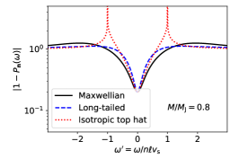
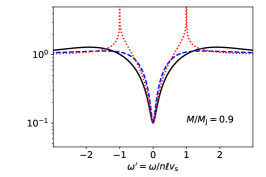
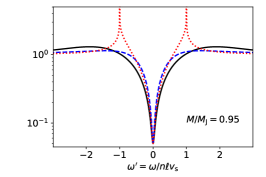
Figure 1: Modulus of the dielecric function $\epsilon_{\bf n}(\omega)\equiv 1-P_{\bf n}(\omega)$ for cube masses $0.8M_{\rm J}$ (left), $0.9M_{\rm J}$ (middle) and $0.95M_{\rm J}$ (right): the cube’s response to an imposed wave of frequency $\omega$ is proportional to $(1-P_{\bf n}(\omega))^{-1}$. Here $|{\bf n}|=1$.

Figure 1 shows how the dielectric function $\epsilon_{\bf n}(\omega)\equiv 1-P_{\bf n}(\omega)$ of the $|{\bf n}|=1$ response varies with the cube’s mass for the Maxwellian, long-tailed and isotropic top-hat DFs: from equations (20) and (23) the amplitude of the response to an imposed $\Phi^{\rm e}_{\bf n}={\rm e}^{-{\rm i}\omega\tau}$ wave is proportional to $1/\epsilon_{\bf n}(\omega)$. As the cube’s mass approaches the appropriate Jeans mass it responds more and more vigorously to low-$\omega$ waves. For fixed $\omega$ the polarizability (23) scales as $1/n^{2}$, which means that the magnitude of the response shrinks rapidly as $|{\bf n}|$ increases.

3 Application to dynamical friction

Now we turn to the problem of a cube being perturbed by a satellite of mass $M_{\rm p}$ that is launched from ${\bf x}=(0,0,0)$ with velocity ${\bf v}_{\rm p}$. Writing ${\bf J}_{\rm p}\equiv\ell{\bf v}_{\rm p}$, the externally imposed potential due to the satellite is

$$\Phi^{\rm e}_{{\bf n}}(\tau)=\frac{M_{\rm p}V_{\bf n}}{(2\pi)^{3}\ell^{3}}{\rm e}^{-i{\bf n}\cdot{\bf J}_{\rm p}\tau}.$$ (33)

We first consider the case in which ${\bf v}_{\rm p}$ and therefore ${\bf J}_{\rm p}$ are held constant. That is, we use the satellite to “stir” the cube. Then in Section 3.5 below we release the satellite and account for the back reaction of the cube’s response.

An important point to note is that, to linear order, this stirring imparts no net momentum to the cube’s stars, nor does it heat them: the momentum and energy of the cube’s response are set by the velocity moments of $f_{(0,0,0)}({\bf J})$, which, from the full CBE (LABEL:eq:fullCBE), can develop only through the nonlinear coupling of $f_{{\bf m}}$ with $\Phi_{-{\bf m}}$.

3.1 Steady-state linear response

To simplify the problem we suppose that the stirred system settles into a dynamical equilibrium, in which the response is related to the stimulus (33) by the time-independent relation

$$\Phi^{f}_{\bf n}=r_{\bf n}\Phi^{\rm e}_{{\bf n}},$$ (34)

where the complex coefficient $r_{\bf n}$ gives the amplitude and phase of the ${\bf n}^{\rm th}$ mode of the potential response with respect to the stimulus. We can find $r_{\bf n}$ by substituting (34) into our expression (20) for $\Phi^{f}_{\bf n}(\tau)$ and rearranging. If we omit the self-gravity of the response by taking $\Phi=\Phi^{\rm e}$ in the integrand of (20), then we obtain

$$\Phi^{f}_{\bf n}=P_{\bf n}({\bf n}\cdot{\bf J}_{\rm p})\Phi^{\rm e}_{\bf n},$$ (35)

where $P_{\bf n}(\omega)$ is the polarizability (23). This $P_{\bf n}({\bf n}\cdot{\bf J}_{\rm p})\Phi_{\bf n}^{\rm e}$ is the so-called “undressed” response, because it does not account for the “dressing” that the response itself contributes to the potential. On the other hand, it is just as easy to include the self gravity of the response by taking $\Phi=\Phi^{\rm e}+\Phi^{f}$ in the integrand of (20). Then, after some rearrangement, we obtain the “dressed” response potential as

$$\Phi^{f}_{\bf n}=\frac{P_{\bf n}({\bf n}\cdot{\bf J}_{\rm p})}{1-P_{\bf n}({\bf n}\cdot{\bf J}_{\rm p})}\Phi^{\rm e}_{\bf n}.$$ (36)

The electrostatic analogue of this equation is $-{\bf P}=(P/\epsilon){\bf D}$, where ${\bf P}$ is the polarization vector, ${\bf D}$ the electric displacement, and $\epsilon=1-P$ is the permittivity or dielectric function.

We now have everything we need to calculate the steady-state dynamical friction force in the following. The galaxy’s response $\Phi^{f}({\mathchoice{\hbox{{\gkvecten\char 18\relax}}}{\hbox{{\gkvecten\char 18\relax}}}{\hbox{{\gkvecseven\char 18\relax}}}{\hbox{{\gkvecseven\char 18\relax}}}},\tau)=\sum_{\bf n}\Phi^{f}_{\bf n}(\tau){\rm e}^{{\rm i}{\bf n}\cdot{\mathchoice{\hbox{{\gkvecten\char 18\relax}}}{\hbox{{\gkvecten\char 18\relax}}}{\hbox{{\gkvecseven\char 18\relax}}}{\hbox{{\gkvecseven\char 18\relax}}}}}$ exerts a drag force $-M_{\rm p}\nabla\Phi^{f}({\mathchoice{\hbox{{\gkvecten\char 18\relax}}}{\hbox{{\gkvecten\char 18\relax}}}{\hbox{{\gkvecseven\char 18\relax}}}{\hbox{{\gkvecseven\char 18\relax}}}}_{\rm p})$ on the satellite. Using (35) and (36), the corresponding deceleration is

$$\begin{split}\dot{\bf J}_{\rm p}&=-\frac{\partial}{\partial{\mathchoice{\hbox{{\gkvecten\char 18\relax}}}{\hbox{{\gkvecten\char 18\relax}}}{\hbox{{\gkvecseven\char 18\relax}}}{\hbox{{\gkvecseven\char 18\relax}}}}}\Phi^{f}({\mathchoice{\hbox{{\gkvecten\char 18\relax}}}{\hbox{{\gkvecten\char 18\relax}}}{\hbox{{\gkvecseven\char 18\relax}}}{\hbox{{\gkvecseven\char 18\relax}}}}_{\rm p})\\ &={\rm i}\sum_{{\bf n}}\frac{M_{\rm p}V_{\bf n}}{(2\pi\ell)^{3}}{\bf n}\times\begin{cases}P_{\bf n}({\bf n}\cdot{\bf J}_{\rm p}),&\hbox{undressed,}\\ \frac{P_{\bf n}({\bf n}\cdot{\bf J}_{\rm p})}{1-P_{\bf n}({\bf n}\cdot{\bf J}_{\rm p})},&\hbox{dressed}.\end{cases}\end{split}$$ (37)

For later use (Section 5) we note that the DF response $\tilde{f}_{\bf n}({\bf k})$ can be obtained in the same way by assuming that it behaves as

$$\frac{MV_{\bf n}\tilde{f}_{\bf n}({\bf k})}{\ell^{3}}=r_{\bf n}({\bf k})\Phi^{\rm e}_{\bf n},$$ (38)

which is the steady-state assumption (34) generalised to ${\bf k}\neq{\bf 0}$ by having a ${\bf k}$-dependent response coefficient $r_{\bf n}({\bf k})$. Substituting this expression for $\tilde{f}_{\bf n}({\bf k})$ into equation (21) with $\Phi=\Phi^{\rm e}$, the response DF $\tilde{f}_{\bf n}({\bf k})$ in the undressed case is given by

$$\frac{MV_{\bf n}\tilde{f}_{\bf n}({\bf k})}{\ell^{3}}=\tilde{P}_{\bf n}({\bf n}\cdot{\bf J}_{\rm p},{\bf k})\Phi^{\rm e}_{\bf n},$$ (39)

while in the self-consistent, dressed case ($\Phi=\Phi^{\rm e}+\Phi^{f}$) it is given by

$$\frac{MV_{\bf n}\tilde{f}_{\bf n}({\bf k})}{\ell^{3}}=\frac{\tilde{P}_{\bf n}({\bf n}\cdot{\bf J}_{\rm p},{\bf k})}{1-P_{\bf n}({\bf n}\cdot{\bf J}_{\rm p})}\Phi^{\rm e}_{\bf n},$$ (40)

where, in both cases, the ${\bf k}$-dependent polarizability is

$$\tilde{P}_{\bf n}(\omega,{\bf k})\equiv-\frac{MV_{\bf n}}{\ell}\int_{0}^{\infty}[{\bf n}\cdot{\bf k}+{\bf n}^{2}\tau]{\rm e}^{{\rm i}\omega\tau}\tilde{F}({\bf k}+{\bf n}\tau)\,{\rm d}\tau.$$ (41)

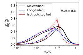
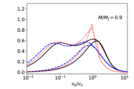
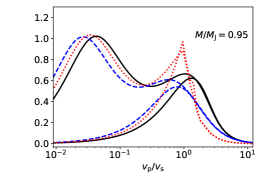
Figure 2: The deceleration from dynamical friction (37) experienced when pulling a satellite of mass $M_{\rm p}$ through various cubes with constant speed $v_{\rm p}$. From left to right, the panels plot results for cubes of mass 0.8, 0.9 and 0.95 times the Jeans mass $M_{\rm J}$ (equations 28, 32). Within each panel the pair of solid curves plot results for cubes with a Maxwellian DF, the upper curve showing the deceleration calculated from the dressed response of the cube to the satellite (that is, accounting for the self-gravity of the response), the lower from the undressed response (that is, ignoring the self gravity of the response). The dashed and dotted curves plot corresponding results for the long-tailed and isotropic top-hat DFs, respectively.

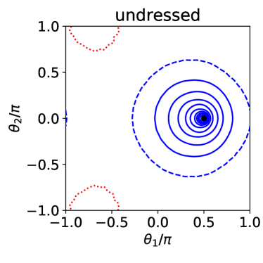
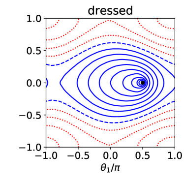
Figure 3: Response density, projected along the $\theta_{3}$ axis, for a satellite dragged with speed $J_{1}=0.3v_{\rm s}$ through a cube of mass $M=0.8M_{\rm J}$ with a Maxwellian DF. The satellite’s position is marked by the heavy black dot. The panel on the left shows the undressed response, the panel on the right the dressed response. The same, linearly-spaced, contour levels are used in both panels. Solid contours denote positive projected density, dotted contours negative density.

3.2 Chandrasekhar’s formula

In the undressed case, the expression (37) for the drag simplifies if the velocity distribution within the cube is isotropic (that is, if $F({\bf J})=F(|{\bf J}|)$). Taking $V_{\bf n}$ from (11) and $P_{\bf n}$ from (23) we have that

$$\dot{\bf J}_{\rm p}=-{\rm i}\frac{(4\pi G)^{2}MM_{\rm p}}{(2\pi)^{3}}S,$$ (42)

where $S$ is a sum over the contributions from different wavenumbers:

$$S=\sum_{\bf n}\frac{{\bf n}}{n^{2}}\int_{0}^{\infty}\tau{\rm e}^{{\rm i}{\bf n}\cdot{\bf J}_{\rm p}\tau}\tilde{F}({\bf n}\tau)\,{\rm d}\tau.$$ (43)

Introducing spherical polar coordinates $(n,\theta,\phi)$ for ${\bf n}$ with the polar axis parallel to ${\bf J}_{\rm p}$ and then approximating the sum over ${\bf n}$ as an integral, we have

$$\begin{split}S\simeq 2\pi\log\left(\frac{n_{\rm max}}{n_{\rm min}}\right)\frac{{\bf J}_{\rm p}}{|{\bf J}_{\rm p}|}\int_{0}^{\infty}{\rm d}k\int_{-1}^{+1}{\rm d}\mu\,\mu{\rm e}^{{\rm i}k\mu J_{\rm p}}k\tilde{F}(k),\end{split}$$ (44)

in which $\mu=\cos\theta$ and $k=n\tau$. Similarly, expressing equation (14) in spherical polar coordinates gives

$$\tilde{F}(k)=2\pi\int_{0}^{\infty}{\rm d}J\,J^{2}F(J)\int_{-1}^{+1}{\rm e}^{-{\rm i}kJ\mu^{\prime}}\,{\rm d}\mu^{\prime}.$$ (45)

Substituting this $\tilde{F}(k)$ into (44), performing the integral over $k$, then $\mu^{\prime}$ and finally $\mu$, our expression (42) for the frictional deceleration in the undressed case becomes

$$\dot{\bf J}_{\rm p}=-(4\pi G)^{2}MM_{\rm p}\log\left(\frac{n_{\rm max}}{n_{\rm min}}\right)\frac{{\bf J}_{\rm p}}{J_{\rm p}^{3}}\int_{0}^{J_{\rm p}}F(J)J^{2}\,{\rm d}J.$$ (46)

This is identical to the usual Chandrasekhar dynamical friction formula (e.g., Binney & Tremaine, 2008; Chavanis, 2013b) with $\log(n_{\rm max}/n_{\rm min})$ playing the role of the Coloumb logarithm, $\log\Lambda$. An important difference, however, is that the usual derivation of the formula assumes local two-body encounters and integrates them exactly, which removes the small-scale cutoff. In our derivation, the unperturbed orbits are straight lines, not two-body hyperbolae; to obtain the inner cutoff correctly we would need to include the $O(\epsilon^{2})$ nonlinear response.

3.3 Examples of the steady-state response

Figure 2 plots how the drag from dynamical friction (37) depends on the perturber’s speed $v_{\rm p}=J_{\rm p}/\ell$ and on the mass of the cube, $M/M_{\rm J}$ for each of the stable DFs listed in Table 1. For these curves we have taken $n_{\rm min}=1$ and $n_{\rm max}=18\simeq GM/\ell v_{\rm s}^{2}$. Figure 3 shows a typical example of the density response from which this drag is computed, demonstrating that the dressed response is much stronger than the undressed one.

Although we do not plot it here, the drag computed from the undressed response agrees very well with the Chandrasekhar dynamical friction formula (46). The only notable difference is that the Chandrasekhar formula predicts a sharp cutoff in the drag when $v_{\rm p}>v_{\rm s}$ in the isotropic top-hat model: according to it stars that move faster than the satellite should not contribute to the frictional force. Figure 2 shows that in our sum over discrete spatial modes ${\bf n}$ this cutoff for the isotropic top-hat model is softened slightly, with further signs of the discreteness occuring when $v_{\rm p}$ is an integer multiple of $v_{\rm s}$.

In the undressed models the frictional deceleration scales linearly with both $M$ and $M_{\rm p}$. When dressing is included, however, as $M\to M_{\rm J}$ the system becomes increasingly responsive to the perturbing satellite: instead of remaining close to 1 everywhere, the magnitude of the dielectric function $1-P_{\bf n}({\bf n}\cdot{\bf J}_{\rm p})$ can approach 0, leading to an arbitrarily large response (36). This is particularly noticeable for slowly moving satellites with $v_{\rm p}\ll v_{\rm s}$. The right-hand panel of Figure 2 shows that the undressed calculation can underestimate the friction by orders of magnitude when $v_{\rm p}\sim 0.1v_{\rm s}$ for all three DFs. For a satellite moving with ${\bf v}_{\rm p}=(0,0,v_{\rm p})$ the dressing predominantly affects the ${\bf n}=(0,0,\pm 1)$ contributions to the response. The contribution to the other modes is weaker than the undressed response.

We note that the deceleration due to dynamical friction depends mostly on $M/M_{\rm J}$, on the speed of the satellite compared to typical stars $v_{\rm p}/v_{\rm s}$, and on whether or not one includes dressing. The shape of the cube’s $F({\bf v})$ distribution is a smaller effect, the most noticeable difference among the three DFs being in the detailed behaviour of the deceleration around $v_{\rm p}/v_{\rm s}\simeq 1$ in the isotropic top-hat model.

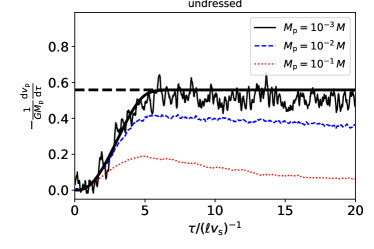
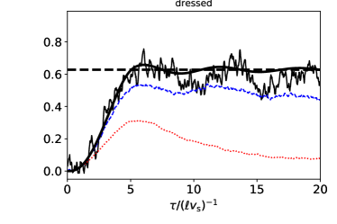
Figure 4: Time evolution of the friction experienced by a satellite that is pulled with constant speed $V_{\rm p}=v_{\rm s}$ through a cube of mass $M=0.9M_{\rm J}$ with a Maxwellian DF. The satellite’s mass grows with time according to (47) over $t=5$ time units. The left and right panels show the drag force that the cube’s undressed and dressed response, respectively, exert on the satellite, normalized by the square of the satellite’s final mass. The heavy solid curves plot results obtained by solving the linear Volterra equation (20). At late times these are in excellent agreement with the steady-state prediction (37) (horizontal dashed line). For comparison, the jagged curves plot the drag measured from $N$-body simulations of the cube’s nonlinear response for satellites that grow to masses $M_{\rm p}=10^{-3}\,M$, $10^{-2}\,M$ and $10^{-1}\,M$. The simulations use $N=10^{8}$ particles to sample the the cube’s DF.

3.4 Time-dependent response: stirring

In obtaining the results above we have assumed (equation 34) that a new equilibrium DF is established within the cube: that is, that $f({\bf x},{\bf v})$ is constant in a frame that moves with the satellite’s constant stirring speed ${\bf v}_{\rm p}$. The most immediate way of testing this assumption is by using equation (20) to obtain the time-dependent response of the cube to a satellite that is introduced from time $\tau=0$.

The satellite’s influence enters through the $\Phi_{\bf n}(\tau^{\prime})$ factor in the integrand of (20). We introduce the satellite slowly, its mass growing as

$$\begin{split}M_{\rm p}(\tau)&=M_{\rm p,final}\,\mu\left(\frac{\tau}{\tau_{\rm grow}}\right),\\ \end{split}$$ (47)

with $\tau_{\rm grow}=5/\ell v_{\rm s}$ and

$$\mu(s)=\begin{cases}0,&s<0,\\ 3s^{2}-2s^{3},&0\leq s\leq 1,\\ 1,&s>1.\end{cases}$$ (48)

To solve (20) we use the trapezoidal rule with step $\Delta\tau=0.01/\ell v_{\rm s}$ to approximate the integral on the right-hand side as a sum over the values of $\Phi_{\bf n}$ at discrete times $\tau=0$, $\Delta\tau$, …., $j\Delta\tau$. Rearranging this gives an expression for $\Phi_{\bf n}^{f}(j\Delta\tau)$ as a sum over the values of $\Phi_{\bf n}$ at earlier times $\tau=0$, $\Delta\tau$, …, $(j-1)\Delta\tau$ and of $\Phi_{\bf n}^{\rm e}$ at time $j\Delta\tau$.

The heavy solid curve in Figure 4 shows a typical example of how the friction experienced by the satellite develops over time according to this linear calculation. The introduction of the satellite excites some oscillations in the cube. Once these have damped, the long-term response is in excellent agreement with the steady-state prediction from (37). The larger $M/M_{\rm J}$ is, the longer this initial ringing takes to die away.

The same Figure plots the friction measured from $N$-body simulations that include the full nonlinear response of the cube to the satellite. The simulation method is described in Appendix A. It is clear from the Figure that the linear response calculation described above is not a particularly good approximation to the full nonlinear response for any $M_{\rm p}\lesssim 10^{-2}M$. The most obvious shortcoming of the linear calculation is that it ignores the momentum transferred to the cube’s stars as the satellite is dragged through the system. In the $N$-body simulations this leads to a gradual decrease in the dynamical friction force as the cube’s stars speed up to match the satellite, a phenomenon that is not captured by the linear calculation.

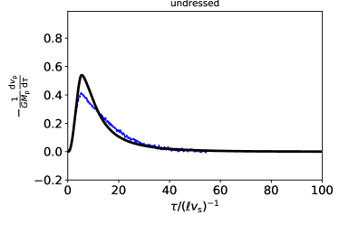
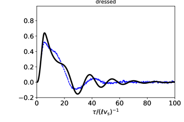
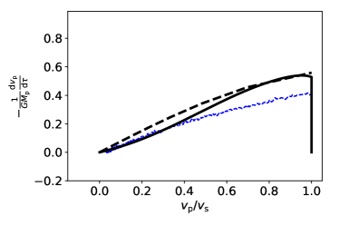
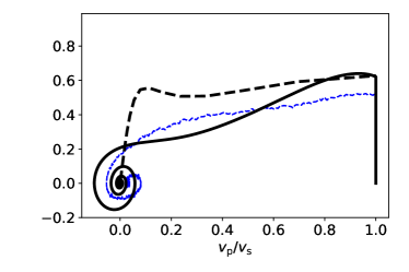
Figure 5: Damping of the motion of a satellite after it has been dragged through a cube of mass $M=0.9\,M_{\rm J}$ with a Maxwellian DF. As in Figure 4, the satellite’s mass grows from 0 to $10^{-2}\,M$ between $t=0$ and $t=5$, during which time it is dragged through the cube with constant speed $v_{\rm p}/v_{\rm s}=1$. At $t=5$ it is released, its subsequent motion governed by the cube’s response. The left and right panels show results when this response is undressed and dressed, respectively The top row shows the time evolution of the drag deceleration, the heavy solid curves giving the predictions of time-dependent linear theory (Section 3.5), the lighter dashed curves measurements from $N$-body simulation. The bottom row shows the same results, but plotted against the satellite’s instantaneous speed $v_{\rm p}$: in this row the satellite starts at $(1,0)$, moves up as it is being dragged, then to the left when released. For comparison the heavy dashed curve plots the deceleration predicted from the “steady-state” formalism of Section 3.1 using only the instantaneous value of $v_{\rm p}$.

3.5 Time-dependent response: damping

In the preceding calculations we have supposed that the satellite is pulled through the cube with constant velocity ${\bf v}_{\rm p}$. What would happen if we were to release the satellite? To investigate this we stir the cube by dragging the satellite through it to build up a wake as before. Then at some $\tau=\tau_{\rm release}$ we let go of the satellite and follow the subsequent evolution of the coupled satellite-plus-wake system. We use the following leapfrog integrator for the satellite’s motion at times $\tau\geq\tau_{\rm release}$:

$$\begin{split}{{\mathchoice{\hbox{{\gkvecten\char 18\relax}}}{\hbox{{\gkvecten\char 18\relax}}}{\hbox{{\gkvecseven\char 18\relax}}}{\hbox{{\gkvecseven\char 18\relax}}}}_{\rm p}}\left(\tau+{\scriptstyle\frac{1}{2}}\Delta\tau\right)&={{\mathchoice{\hbox{{\gkvecten\char 18\relax}}}{\hbox{{\gkvecten\char 18\relax}}}{\hbox{{\gkvecseven\char 18\relax}}}{\hbox{{\gkvecseven\char 18\relax}}}}_{\rm p}}(\tau)+{\scriptstyle\frac{1}{2}}{{\bf J}_{\rm p}}(\tau)\Delta\tau,\\ {\bf J}_{\rm p}(\tau+\Delta\tau)&={\bf J}_{\rm p}-{\rm i}\sum_{\bf n}{\bf n}\Phi^{f}_{\bf n}\left(\tau+{\scriptstyle\frac{1}{2}}\Delta\tau\right){\rm e}^{{\rm i}{\bf n}\cdot{\mathchoice{\hbox{{\gkvecten\char 18\relax}}}{\hbox{{\gkvecten\char 18\relax}}}{\hbox{{\gkvecseven\char 18\relax}}}{\hbox{{\gkvecseven\char 18\relax}}}}_{\rm p}(\tau+{\scriptscriptstyle\frac{1}{2}}\Delta\tau)}\Delta\tau,\\ {{\mathchoice{\hbox{{\gkvecten\char 18\relax}}}{\hbox{{\gkvecten\char 18\relax}}}{\hbox{{\gkvecseven\char 18\relax}}}{\hbox{{\gkvecseven\char 18\relax}}}}_{\rm p}}\left(\tau+\Delta\tau\right)&={{\mathchoice{\hbox{{\gkvecten\char 18\relax}}}{\hbox{{\gkvecten\char 18\relax}}}{\hbox{{\gkvecseven\char 18\relax}}}{\hbox{{\gkvecseven\char 18\relax}}}}_{\rm p}}\left(\tau+{\scriptstyle\frac{1}{2}}\Delta\tau\right)+{\scriptstyle\frac{1}{2}}{{\bf J}_{\rm p}}(\tau)\Delta\tau.\\ \end{split}$$ (49)

The potential $\Phi_{\bf n}^{f}(\tau+\frac{1}{2}\Delta\tau)$ in the middle, “kick”, step is calculated as described in Section 3.4 above, taking $\Phi^{\rm e}_{\bf n}(\tau^{\prime})$ from the ${\mathchoice{\hbox{{\gkvecten\char 18\relax}}}{\hbox{{\gkvecten\char 18\relax}}}{\hbox{{\gkvecseven\char 18\relax}}}{\hbox{{\gkvecseven\char 18\relax}}}}_{\rm p}(\tau^{\prime})$ obtained from the new satellite position ${\mathchoice{\hbox{{\gkvecten\char 18\relax}}}{\hbox{{\gkvecten\char 18\relax}}}{\hbox{{\gkvecseven\char 18\relax}}}{\hbox{{\gkvecseven\char 18\relax}}}}_{\rm p}(\tau+{\scriptstyle\frac{1}{2}}\Delta\tau)$.

Figure 5 shows how the frictional deceleration evolves for a satellite of mass $10^{-2}\,M_{\rm J}$ that is released with $v_{\rm p}/v_{\rm s}=1$ within a Maxwellian cube of mass $M=0.9\,M_{\rm J}$. If one considers only the undressed response then this evolution is simple: the satellite slows down until it comes to rest. The dressed response is more interesting, however: as the satellite slows down, the response that is has induced in the cube’s stars overtakes it, causing it to speed up again, overtaking the response, leading to damped oscillations in $v_{\rm p}(\tau)$. The dashed curve in the lower right panel of Figure 5 shows that the steady-state approximation used in Section 3.1 completely fails to capture this evolution.

Qualitatively the same phenomena are observed in $N$-body simulations of the same system, the most notable difference being how the $N$-body simulations exhibit smaller-amplitude oscillations and converge to a final $v_{\rm p}\neq 0$ that arises from the momentum imparted to the cube’s stars before the satellite is released.

4 van Kampen modes

In section 2.4 we derived the dispersion relation (24), the solutions to which are the frequencies $\omega$ of the self-sustaining waves that the cube admits. In general these frequencies are complex, which means that these waves grow exponentially in either the forward or backward time direction. These waves – the so-called Landau modes – are not the only waves admitted by the cube, however.

Consider a self-consistent oscillation of an isolated cube ($\Phi^{\rm e}=0$) with real frequency $\omega$:

$$\begin{split}\tilde{f}_{\bf n}({\bf k},\tau|\omega)&=\tilde{f}_{{\bf n}}({\bf k}|\omega){\rm e}^{-{\rm i}\omega\tau},\\ \Phi_{\bf n}(\tau|\omega)&=\tilde{\Phi}_{{\bf n}}(\omega){\rm e}^{-{\rm i}\omega\tau},\end{split}$$ (50)

in which, by Poisson’s equation (19), $\tilde{\Phi}_{{\bf n}}(\omega)=(MV_{\bf n}/\ell^{3})\tilde{f}_{{\bf n}}({\bf 0}|\omega)$. Let $k_{\parallel}$ be the component of ${\bf k}$ that is parallel to ${\bf n}$. Then ${\bf n}\cdot{\bf k}=nk_{\parallel}$ and the linearized Fourier-transformed CBE (15) for $\tilde{f}_{\bf n}({\bf k}_{\perp},k_{\parallel}|\omega)$ becomes

$${\rm i}\omega\tilde{f}_{{\bf n}}({\bf k}_{\perp},k_{\parallel}|\omega)+n\frac{\partial\tilde{f}_{{\bf n}}}{\partial k_{\parallel}}({\bf k}_{\perp},k_{\parallel}|\omega)-nk_{\parallel}\,\ell^{2}\tilde{F}({\bf k}_{\perp},k_{\parallel})\tilde{\Phi}_{{\bf n}}(\omega)=0.$$ (51)

The solutions are

$$\begin{split}&\tilde{f}_{{\bf n}}({\bf k}_{\perp},k_{\parallel}|\omega)={\rm e}^{-{\rm i}\omega k_{\parallel}/n}\times\\ &\quad\left[\tilde{f}^{\perp}_{{\bf n}}({\bf k}_{\perp}|\omega)+\tilde{\Phi}_{{\bf n}}(\omega)\ell^{2}\int_{0}^{k_{\parallel}}{\rm e}^{{\rm i}\omega k_{\parallel}^{\prime}/n}k_{\parallel}^{\prime}\tilde{F}({\bf k}_{\perp},k_{\parallel}^{\prime})\,{\rm d}k_{\parallel}^{\prime}\right],\end{split}$$ (52)

in which the only constraint on the constant of integration $\tilde{f}^{\perp}_{{\bf n}}({\bf k}_{\perp}|\omega)$ is that $\tilde{f}^{\perp}_{{\bf n}}({\bf 0}|\omega)=\tilde{f}_{{\bf n}}({\bf 0}|\omega)$.

These are the (Fourier-transformed) van Kampen (1955) modes of the cube. To show this explicitly, notice that $k_{\parallel}\tilde{F}({\bf k}_{\perp},k^{\prime}_{\parallel})$ is the Fourier transform of $\partial F/\partial k^{\prime}_{\parallel}$. Then performing the integral over $k_{\parallel}^{\prime}$ gives

$$\begin{split}&\tilde{f}_{{\bf n}}({\bf k}_{\perp},k_{\parallel}|\omega)={\rm e}^{-{\rm i}\omega k_{\parallel}/n}\tilde{f}^{\perp}_{{\bf n}}({\bf k}_{\perp}|\omega)\\ &\quad+\tilde{\Phi}_{{\bf n}}(\omega)\ell^{2}{\rm e}^{-{\rm i}\omega k_{\parallel}/n}\int{\rm d}^{3}{\bf J}^{\prime}\frac{1-{\rm e}^{{\rm i}k_{\parallel}(\omega-{\bf n}\cdot{\bf J}^{\prime})/n}}{\omega-{\bf n}\cdot{\bf J}^{\prime}}{\bf n}\cdot\frac{\partial F}{\partial{\bf J}^{\prime}}.\end{split}$$ (53)

The integrand is well behaved when the denominator $\omega-{\bf n}\cdot{\bf J}^{\prime}$ vanishes. That means that we may excise the plane $\omega-{\bf n}\cdot{\bf J}^{\prime}=0$ from the integration range without changing the value of the integral. So, carrying out the inverse Fourier transform after splitting the integral into two produces

$$\begin{split}&\frac{1}{n}f_{\bf n}({\bf J}|\omega)=-\tilde{\Phi}_{\bf n}\ell^{2}\frac{1}{\omega-{\bf n}\cdot{\bf J}}{\bf n}\cdot\frac{\partial F}{\partial{\bf J}}\\ &\quad+\left[f^{\perp}_{\bf n}({\bf J}_{\perp}|\omega)+\tilde{\Phi}_{\bf n}(\omega)\ell^{2}{\cal P}\int\frac{{\rm d}^{3}{\bf J}^{\prime}}{\omega-{\bf n}\cdot{\bf J}^{\prime}}\right]\delta\left({{\bf n}\cdot{\bf J}-\omega}\right),\\ &\end{split}$$ (54)

where ${\cal P}$ denotes the Cauchy principal value. Up to a multiplicative factor this agrees with the expression for the DF of a van Kampen mode given by equation (4) of Box 5.1 of Binney & Tremaine (2008).

The van Kampen modes (52) do not satisfy the dispersion relation (24). The reason for this is simple, although possibly not immediately obvious: we obtained the dispersion relation from the integral equation (20), which in turn came from integrating the (Fourier-transformed) CBE (15) with an implicit assumption that $\tilde{f}_{\bf n}({\bf k})\to 0$ as $|{\bf k}|\to\infty$. The van Kampen modes (52) do not vanish as $|{\bf k}|\to\infty$ and therefore do not satisfy the dispersion relation. For the same reason they are singular when viewed in action or velocity space. The relationship between waves that satisfy the dispersion relation (the Landau modes) and van Kampen modes is discussed in Lau & Binney (2021).

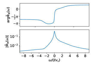
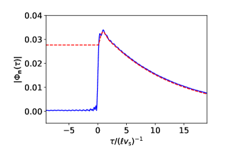
Figure 6: Left: Spectrum $\tilde{\Phi}_{\bf n}^{+}(\omega)$ (equation 61) of the van Kampen-mode expansion of the ${\bf n}=(0,0,1)$ component of the wake caused by a satellite moving with speed ${\bf v}_{\rm p}=(0,0,2)v_{\rm s}$ in a cube of mass $M=0.9M_{\rm J}$ with a Maxwellian DF. Right: the time-dependent potential $\Phi_{\bf n}^{+}(\tau)$ reconstructed from modes having $|\omega|<10$ (solid curve) compared to the numerical solution of the Volterra equation (20) (dashed curve) in which a slowly grown satellite is suddenly removed at $t=0$.

Standard properties of Fourier transforms guarantee that any well-behaved perturbation $f_{\bf n}({\bf k},\tau)$ or $\tilde{f}_{\bf n}({\bf k},\tau)$ can be expressed as a superposition of van Kampen modes (52). Here is how to perform this decomposition given a snapshot $f_{\bf n}({\bf J},\tau=0)$ at $\tau=0$. Integrate the characteristic equation (17) from this $\tau=0$ initial condition to obtain

$$\begin{split}\Phi_{\bf n}(\tau)&=\frac{MV_{\bf n}}{\ell^{3}}\tilde{f}_{\bf n}({\bf n}\tau,0)\\ &-\frac{MV_{\bf n}}{\ell}\int_{0}^{\tau}{\rm d}\tau^{\prime}\,{\bf n}^{2}(\tau-\tau^{\prime})\tilde{F}({\bf n}(\tau-\tau^{\prime}))\Phi_{\bf n}(\tau^{\prime}).\end{split}$$ (55)

and split $\Phi_{\bf n}(\tau)=\Phi^{+}_{\bf n}(\tau)+\Phi^{-}_{\bf n}(\tau)$, where $\Phi^{+}_{\bf n}(\tau)$ is zero for $\tau<0$ and $\Phi^{-}_{\bf n}(\tau)$ is zero for $\tau>0$. Then (55) becomes a pair of integral equations, one for $\Phi^{+}_{\bf n}(\tau)$ that holds only for $\tau\geq 0$, the other for $\Phi^{-}_{\bf n}(\tau)$ that holds only for $\tau\leq 0$. Introduce the Fourier transforms

$$\tilde{\Phi}_{\bf n}(\omega)=\int_{-\infty}^{\infty}{\rm e}^{{\rm i}\omega\tau}\Phi_{\bf n}(\tau)\,{\rm d}\tau;\quad\Phi_{\bf n}(\tau)=\frac{1}{2\pi}\int_{-\infty}^{\infty}{\rm e}^{-{\rm i}\omega\tau}\tilde{\Phi}_{\bf n}(\omega)\,{\rm d}\omega.$$ (56)

Fourier transforming the integral equation (55) for $\Phi^{+}_{\bf n}(\tau)$ gives

$$\begin{split}\tilde{\Phi}^{+}_{\bf n}(\omega)&=\frac{MV_{\bf n}}{\ell^{3}}\int_{0}^{\infty}{\rm e}^{{\rm i}\omega\tau}\tilde{f}_{\bf n}({\bf n}\tau,0)\,{\rm d}\tau+P_{\bf n}(\omega)\tilde{\Phi}^{+}_{\bf n}(\omega),\end{split}$$ (57)

where we have used $\tilde{\Phi}^{+}_{\bf n}(\tau)=0$ for $\tau<0$ to extend the lower limit of the integral in the second term of (55) from $\tau=0$ to $\tau\to-\infty$. Rearranging, we have that $\Phi^{+}_{\bf n}(\tau)$ is superposition of modes $\tilde{\Phi}^{+}_{\bf n}(\omega){\rm e}^{-{\rm i}\omega\tau}$ with amplitudes

$$\begin{split}\tilde{\Phi}_{\bf n}^{+}(\omega)&=\frac{2\pi}{1-P_{{\bf n}}(\omega)}\frac{MV_{\bf n}}{\ell^{3}}\int f_{\bf n}({\bf J},0)\delta(\omega-{\bf n}\cdot{\bf J})\,{\rm d}^{3}{\bf J}.\end{split}$$ (58)

The ${\rm e}^{-{\rm i}\omega\tau}$ time dependence of the modes means that $\tilde{\Phi}_{\bf n}^{-}(\omega)=[\tilde{\Phi}_{\bf n}^{+}(\omega)]^{\star}$ and therefore that $\tilde{\Phi}_{\bf n}(\omega)=\tilde{\Phi}^{+}_{\bf n}(\omega)+\tilde{\Phi}_{\bf n}^{-}(\omega)=2\mathop{\hbox{Re}}\tilde{\Phi}_{\bf n}^{+}(\omega)$.

Simiarly, we can find $\tilde{f}_{\bf n}({\bf k}_{\perp}|\omega)$ by first expressing our initial condition as a superposition of modes,

$$\tilde{f}_{\bf n}({\bf k},0)=\frac{1}{2\pi}\int{\rm d}\omega^{\prime}\,\tilde{f}_{\bf n}({\bf k}_{\perp},k_{\parallel}|\omega^{\prime}).$$ (59)

Multiplying this by ${\rm e}^{{\rm i}\omega k_{\parallel}/n}$, integrating over $k_{\parallel}$ and rearranging the result we have that

$$\begin{split}\tilde{f}_{\bf n}^{\perp}({\bf k}_{\perp}|\omega)&=\frac{1}{n}\int_{-\infty}^{\infty}\tilde{f}_{\bf n}({\bf k}_{\perp},k_{\parallel},0){\rm e}^{{\rm i}\omega k_{\parallel}/n}{\rm d}k_{\parallel}\\ &\quad+\frac{\ell^{3}}{MV_{\bf n}}\tilde{\Phi}_{\bf n}(\omega)P_{\bf n}(\omega),\end{split}$$ (60)

which reduces to (57) when ${\bf k}_{\perp}={\bf 0}$.

For illustration, consider the steady-state wake produced by a satellite of mass $M_{\rm p}$ that moves within the cube at constant speed ${\bf v}_{\rm p}$ for $\tau<0$. Suppose that the satellite has arrived at ${\mathchoice{\hbox{{\gkvecten\char 18\relax}}}{\hbox{{\gkvecten\char 18\relax}}}{\hbox{{\gkvecseven\char 18\relax}}}{\hbox{{\gkvecseven\char 18\relax}}}}={\bf 0}$ at time $\tau=0$, at which point it is suddenly removed. At that instant the perturbed DF of the cube is given by equation (40) with $\Phi^{\rm e}_{\bf n}=M_{\rm p}V_{\bf n}/(2\pi)^{3}$. Substituting this $\tilde{f}_{\bf n}({\bf k},0)$ into (58) gives

$$\begin{split}\tilde{\Phi}_{\bf n}^{+}(\omega)&=-\frac{{\rm i}n^{2}M_{\rm p}V_{\bf n}}{(2\pi)^{3}\ell^{3}}\frac{1}{1-P_{\bf n}(\omega)}\frac{1}{1-P_{\bf n}({\bf n}\cdot{\bf J}_{\rm p})}\\ &\quad\times\frac{P_{\bf n}(\omega)-P_{\bf n}({\bf n}\cdot{\bf J}_{\rm p})}{\omega-{\bf n}\cdot{\bf J}_{\rm p}}.\end{split}$$ (61)

The left panel of Figure 6 shows this $\tilde{\Phi}_{\bf n}^{+}(\omega)$ for ${\bf n}=(0,0,1)$ in the case of a satellite moving with ${\bf v}_{\rm p}=(0,0,2)v_{\rm s}$ in a cube of mass $M=0.9M_{\rm J}$ with a Maxwellian velocity distribution. The right panel plots the positive-time potential $\Phi^{+}_{\bf n}(\tau)$ reconstructed from (61) and compares to the results obtained from the Volterra equation (20) in which the satellite grows slowly over $-80<\tau/(\ell v_{\rm s})^{-1}<-20$, has constant mass for $-20<\tau/(\ell v_{\rm s})^{-1}<0$ and then is removed at $\tau=0$.

5 Quasi-linear evolution of an isolated $N$-body system

So far we have treated the cube as a purely collisionless system. Now let us consider a cube composed of $N$ equal-mass stars, each of mass $M/N$. Each star will induce a wake as it passes through the cube. Bearing in mind the caveats found in the time-dependent calculations of Sections 3.4 and 3.5 we can use the results from Section 3.1 to calculate the net response of the cube to all of these wakes. We model the evolution of the $N$-body system as a superposition of uncorrelated, dressed two-particle interactions, an idea that goes back to Rostoker (1964a, b): see Hamilton (2021) for a lucid overview of the history of this idea, together with another example of its application to the more general case of inhomogeneous systems (Heyvaerts, 2010; Chavanis, 2012c).

We assume that the cube is isolated and not subject to any externally imposed perturbation. Instead, the fluctuations caused by shot noise in the DF will act as an effective “external”, stirring potential, $\Phi^{\rm e}$. That is, the discrete nature of the $N$-body realisation gives rise to a perturbation

$$\rho^{\rm e}({\mathchoice{\hbox{{\gkvecten\char 18\relax}}}{\hbox{{\gkvecten\char 18\relax}}}{\hbox{{\gkvecseven\char 18\relax}}}{\hbox{{\gkvecseven\char 18\relax}}}},t)=\frac{1}{N}\sum_{n=1}^{N}\delta({\mathchoice{\hbox{{\gkvecten\char 18\relax}}}{\hbox{{\gkvecten\char 18\relax}}}{\hbox{{\gkvecseven\char 18\relax}}}{\hbox{{\gkvecseven\char 18\relax}}}}-{\mathchoice{\hbox{{\gkvecten\char 18\relax}}}{\hbox{{\gkvecten\char 18\relax}}}{\hbox{{\gkvecseven\char 18\relax}}}{\hbox{{\gkvecseven\char 18\relax}}}}_{n}(t))-\rho_{0},$$ (62)

in the density of our idealized smooth, collisionless cube: in the $N$-body system the smooth background density $\rho_{0}=\frac{M}{(2\pi)^{3}}$ is replaced by a sum of point masses located at the stars’ positions. We model the stars’ motion as the straight-line orbits they would follow in the unperturbed system. Then the angles of our ensemble of $N$ stars vary with time as ${\mathchoice{\hbox{{\gkvecten\char 18\relax}}}{\hbox{{\gkvecten\char 18\relax}}}{\hbox{{\gkvecseven\char 18\relax}}}{\hbox{{\gkvecseven\char 18\relax}}}}_{n}(\tau)={\bf J}_{n}\tau+{\mathchoice{\hbox{{\gkvecten\char 18\relax}}}{\hbox{{\gkvecten\char 18\relax}}}{\hbox{{\gkvecseven\char 18\relax}}}{\hbox{{\gkvecseven\char 18\relax}}}}_{{\bf n},0}$. The actions ${\bf J}_{\bf n}$ are constant. From equations (9) and (62) or from (33) the stirring potential corresponding to (62) is

$$\Phi^{\rm e}_{{\bf m}}(\tau)=\frac{MV_{\bf m}}{(2\pi)^{3}\ell^{3}N}\sum_{n=1}^{N}{\rm e}^{-{\rm i}{\bf m}\cdot{\mathchoice{\hbox{{\gkvecten\char 18\relax}}}{\hbox{{\gkvecten\char 18\relax}}}{\hbox{{\gkvecseven\char 18\relax}}}{\hbox{{\gkvecseven\char 18\relax}}}}_{n}(\tau)}.$$ (63)

We assume that the cube settles down quickly enough that we can consider each star to be followed by a steady-state wake, as described in Section 3.1. Using equation (36), the full potential, including the contribution from the wakes, is given by

$$\Phi_{{\bf m}}(\tau)=\frac{MV_{\bf m}}{(2\pi)^{3}\ell^{3}N}\sum_{n=1}^{N}\frac{1}{1-P_{\bf m}({\bf m}\cdot{\bf J}_{n})}{\rm e}^{-{\rm i}{\bf m}\cdot{\mathchoice{\hbox{{\gkvecten\char 18\relax}}}{\hbox{{\gkvecten\char 18\relax}}}{\hbox{{\gkvecseven\char 18\relax}}}{\hbox{{\gkvecseven\char 18\relax}}}}_{n}(\tau)}.$$ (64)

Similarly, using (18) and (40), the perturbed DF is given by

$$\begin{split}&\tilde{f}_{{\bf m}}({\bf k},\tau)=\frac{1}{(2\pi)^{3}N}\times\\ &\sum_{n=1}^{N}\Bigg{[}{\rm e}^{-{\rm i}{\bf k}\cdot{\bf J}_{n}}+\frac{\tilde{P}_{\bf m}({\bf m}\cdot{\bf J}_{n},{\bf k})}{1-P_{\bf m}({\bf m}\cdot{\bf J}_{n})}\Bigg{]}{\rm e}^{-{\rm i}{\bf m}\cdot{\mathchoice{\hbox{{\gkvecten\char 18\relax}}}{\hbox{{\gkvecten\char 18\relax}}}{\hbox{{\gkvecseven\char 18\relax}}}{\hbox{{\gkvecseven\char 18\relax}}}}_{n}(\tau)}.\\ \end{split}$$ (65)

The first term in the square brackets comes from the contribution $\delta({\mathchoice{\hbox{{\gkvecten\char 18\relax}}}{\hbox{{\gkvecten\char 18\relax}}}{\hbox{{\gkvecseven\char 18\relax}}}{\hbox{{\gkvecseven\char 18\relax}}}}-{\mathchoice{\hbox{{\gkvecten\char 18\relax}}}{\hbox{{\gkvecten\char 18\relax}}}{\hbox{{\gkvecseven\char 18\relax}}}{\hbox{{\gkvecseven\char 18\relax}}}}_{n})\delta({\bf J}-{\bf J}_{n})$ that each star makes directly to $f({\mathchoice{\hbox{{\gkvecten\char 18\relax}}}{\hbox{{\gkvecten\char 18\relax}}}{\hbox{{\gkvecseven\char 18\relax}}}{\hbox{{\gkvecseven\char 18\relax}}}},{\bf J},\tau)$, the second from the wake that it induces. The perturbed DF $f({\mathchoice{\hbox{{\gkvecten\char 18\relax}}}{\hbox{{\gkvecten\char 18\relax}}}{\hbox{{\gkvecseven\char 18\relax}}}{\hbox{{\gkvecseven\char 18\relax}}}},{\bf J},\tau)$ also has a constant $-F({\bf J})$ term, but that affects only the ${\bf m}=(0,0,0)$ contribution to the Fourier expansion of $f$.

Armed with these expressions for the linearized response we can now use the (nonlinear) characteristic evolution equation (17) to estimate the effect that this shot noise has on the angle-averaged response $f_{(0,0,0)}({\bf J},\tau)$ over many dynamical times. We are more interested in the general properties of this evolution than in the details for any particular realisation of the stellar distribution. So we write (17) as

$$\frac{\partial}{\partial t}\langle\tilde{f}_{(0,0,0)}({\bf k},\tau)\rangle=-\sum_{\bf m}{\bf m}\cdot{\bf k}\left\langle\tilde{f}_{-{\bf m}}({\bf k},\tau)\Phi_{\bf m}(\tau)\right\rangle,$$ (66)

where $\langle\cdot\rangle$ denotes an ensemble average, obtained by averaging over all possible configuration histories of the system. Taking the inverse Fourier transform of this expression yields a continuity equation for $f_{(0,0,0)}({\bf J},t)$,

$$\frac{\partial}{\partial t}\langle f_{(0,0,0)}({\bf J},t)\rangle=-\frac{\partial}{\partial{\bf J}}\cdot{\bf F}({\bf J},t),$$ (67)

in which the flux is given by

$${\bf F}({\bf J},t)\equiv-{\rm i}\sum_{\bf m}{\bf m}\left\langle f_{-{\bf m}}({\bf J},t)\Phi_{\bf m}(t)\right\rangle.$$ (68)

Expressions (66)–(68) would be exact if we were to substitute the nonlinearly evolved $f_{\bf m}({\bf J},\tau)$ and $\Phi_{\bf m}(\tau)$ in the right-hand sides. We only have the linearized approximations (65) and (64) though, in which case the flux (68) becomes a superposition of $O(1/N^{2})$ contributions from uncorrelated dressed two-body interactions.

To carry out the ensemble averaging in (68) we use the following result from Monte Carlo integration. Suppose that points $x_{1},...,x_{N}$ are drawn independently from a pdf $F(x)$ and let $g(x)$ and $h(x)$ be functions of $x$ whose means are zero. Then the ensemble average

$$\begin{split}&\left\langle\sum_{i=1}^{N}g(x_{i})\sum_{j=1}^{N}h(x_{j})\right\rangle\\ &=\left\langle\sum_{i=1}^{N}g(x_{i})h(x_{i})\right\rangle+\left\langle\sum_{i=1}^{N}g(x_{i})\sum_{j\neq i}h(x_{j})\right\rangle\\ &=N\int{\rm d}x\,F(x)g(x)h(x),\end{split}$$ (69)

the second term in the second line vanishing because the $x_{i}$ are independently drawn from $F$. The ensemble averages on the RHS of (66) then become

$$\begin{split}\langle\tilde{f}_{-{\bf m}}\Phi_{\bf m}\rangle&=\frac{MV_{\bf m}}{(2\pi\ell)^{3}N}\int{\rm d}^{3}{\bf J}^{\prime}F({\bf J}^{\prime})\frac{{\rm e}^{-{\rm i}{\bf k}\cdot{\bf J}^{\prime}}}{1-P_{\bf m}({\bf m}\cdot{\bf J}^{\prime})}\\ &+\frac{MV_{\bf m}}{(2\pi\ell)^{3}N}\int{\rm d}^{3}{\bf J}^{\prime}F({\bf J}^{\prime})\frac{\tilde{P}_{-{\bf m}}(-{\bf m}\cdot{\bf J}^{\prime},{\bf k})}{|1-P_{\bf m}({\bf m}\cdot{\bf J}^{\prime})|^{2}},\end{split}$$ (70)

where the denominator in the second term comes from using the relation $P_{-{\bf m}}(-\omega)=P^{\star}_{\bf m}(\omega)$ that follows directly from the definition (23). Taking the inverse Fourier transform of this expression and substituting the resulting $\langle f_{-{\bf m}}\Phi_{\bf m}\rangle$ into (68), the flux can be split into two parts, ${\bf F}={\bf F}_{1}+{\bf F}_{2}$, in which

$${\bf F}_{1}=-{\rm i}\frac{1}{(2\pi\ell)^{3}N}F({\bf J})\sum_{\bf m}{\bf m}\frac{MV_{\bf m}}{1-P_{\bf m}({\bf m}\cdot{\bf J})},$$ (71)

is a “drift” term that depends linearly on $F({\bf J})$, and, using equation (40),

$$\begin{split}&{\bf F}_{2}=-\frac{\pi}{(2\pi\ell)^{3}N\ell}\times\\ &\sum_{\bf m}{\bf m}|MV_{\bf m}|^{2}{\bf m}\cdot\frac{\partial F({\bf J})}{\partial{\bf J}}\int\frac{F({\bf J}^{\prime})\delta({\bf m}\cdot({\bf J}-{\bf J}^{\prime}))}{|1-P_{\bf m}({\bf m}\cdot{\bf J}^{\prime})|^{2}}{\rm d}^{3}{\bf J}^{\prime}\end{split}$$ (72)

is a “diffusive” term that depends on $\partial F/\partial{\bf J}$.

We may turn the expression for ${\bf F}_{1}$ into something that has the same form as that for ${\bf F}_{2}$ by rewriting the sum in (71) as

$$\begin{split}&\sum_{\bf m}{\bf m}\frac{MV_{\bf m}}{1-P_{\bf m}({\bf m}\cdot{\bf J})}=\sum_{\bf m}{\bf m}MV_{\bf m}\frac{1-P_{\bf m}^{\star}({\bf m}\cdot{\bf J})}{|1-P_{\bf m}({\bf m}\cdot{\bf J}|^{2}}\\ &=\frac{1}{2}\sum_{\bf m}{\bf m}MV_{\bf m}-\frac{P_{\bf m}^{\star}({\bf m}\cdot{\bf J})-P^{\star}_{-{\bf m}}(-{\bf m}\cdot{\bf J})}{|1-P_{\bf m}({\bf m}\cdot{\bf J})|^{2}}\\ &=\frac{1}{2}\sum_{\bf m}{\bf m}MV_{\bf m}\frac{MV_{\bf m}^{\star}{\bf m}^{2}\left[\int_{-\infty}^{\infty}\tau{\rm e}^{{\rm i}{\bf m}\cdot{\bf J}\tau}\tilde{F}({\bf m}\tau){\rm d}\tau\right]^{\star}}{\ell|1-P_{\bf m}({\bf m}\cdot{\bf J})|^{2}},\\ \end{split}$$ (73)

where to obtain the last line we have used the definition (23) of $P_{\bf m}(\omega)$. Now notice that the integral in the square brackets can obtained by differentiating the equation

$$\int_{-\infty}^{\infty}{\rm e}^{{\rm i}{\bf m}\cdot{\bf J}\tau}\tilde{F}({\bf m}\tau)\,{\rm d}\tau={(2\pi)}\int F({\bf J}^{\prime})\delta({\bf m}\cdot({\bf J}-{\bf J}^{\prime})){\rm d}^{3}{\bf J}^{\prime}.$$ (74)

Using this in (73) and substituting back into (71) we obtain

$${\bf F}_{1}=\frac{\pi}{(2\pi\ell)^{3}N\ell}\sum_{\bf m}{\bf m}|MV_{\bf m}|^{2}F({\bf J})\int\frac{{\bf m}\cdot\frac{\partial F}{\partial{\bf J}^{\prime}}\delta({\bf m}\cdot({\bf J}-{\bf J}^{\prime}))}{|1-P_{\bf m}({\bf m}\cdot{\bf J}^{\prime})|^{2}}{\rm d}^{3}{\bf J}^{\prime}.$$ (75)

This can be combined with our expression (72) to write the total flux as

$$\begin{split}&{\bf F}=\frac{\pi}{(2\pi\ell)^{3}N\ell}\sum_{\bf m}{\bf m}|MV_{\bf m}|^{2}\times\\ &\int\frac{\delta({\bf m}\cdot({\bf J}-{\bf J}^{\prime}))}{|1-P_{\bf m}({\bf m}\cdot{\bf J}^{\prime})|^{2}}{\bf m}\cdot\left[F({\bf J})\frac{\partial F({\bf J}^{\prime})}{\partial{\bf J}^{\prime}}-F({\bf J}^{\prime})\frac{\partial F({\bf J})}{\partial{\bf J}}\right]{\rm d}^{3}{\bf J}^{\prime}.\end{split}$$ (76)

Replacing ${\bf J}$ by $\ell{\bf v}$ (equation 3) and taking the limit $\ell\to\infty$ of an infinite box, this action flux agrees with the velocity flux for an infinite homogeneous system given by equation (36) of Chavanis (2012b), once we account for the different normalisations used for the DF $F$ and the potential $V_{\bf m}$.

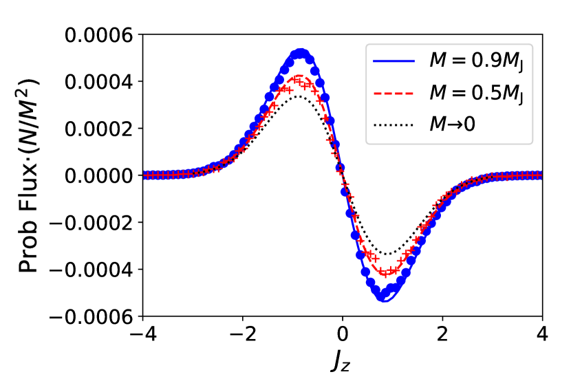
Figure 7: Comparison of the Lenard-Balescu flux predictions (79) against those measured from ensembles of $N$-body simulations for cubes with DF (78) and masses $M=0.9M_{\rm J}$ and $0.5M_{\rm J}$. The fluxes are scaled by $N/M^{2}$ to isolate the effects of the enhancement from particle dressing. The $M\to 0$ curve (dotted) shows the flux obtained when this dressing is turned off.

5.1 Test

The flux (76) vanishes if $F({\bf J})$ is Maxwellian. A more interesting result occurs if we take $F({\bf J})$ to be a sum of Maxwellians though. Writing

$$G({\bf J}|{\bf J}_{0})=\frac{1}{(2\pi)^{3/2}}\exp\left[-\frac{1}{2}({\bf J}-{\bf J}_{0})^{2}\right]$$ (77)

for a unit-dispersion Maxwellian centred on ${\bf J}={\bf J}_{0}$, we take as our DF

$$F({\bf J})=\frac{1}{2(2\pi)^{3}}\left[G({\bf J}|{\bf J}_{0})+G({\bf J}|-{\bf J}_{0})\right].,$$ (78)

a superposition of two Maxwellians, one centred on ${\bf J}_{0}=(0,0,\frac{1}{2})$, the other at $-{\bf J}_{0}$ (see also Chavanis (2012a)). The Lenard–Balescu flux (76) for this DF is

$$\begin{split}{\bf F}=&\frac{\pi}{(2\pi\ell)^{3}N\ell}\sum_{\bf m}\frac{{\bf m}|MV_{\bf m}|^{2}}{|1-P_{\bf m}({\bf m}\cdot{\bf J})|^{2}}\times\\ &\frac{{\bf m}\cdot{\bf J}_{0}}{2(2\pi)^{6}}\left[G({\bf J}|-{\bf J}_{0})G_{\bf m}({\bf J}|{\bf J}_{0})-G({\bf J}|{\bf J}_{0})G_{\bf m}({\bf J}|-{\bf J}_{0})\right],\end{split}$$ (79)

in which

$$\begin{split}G_{\bf m}({\bf J}|{\bf J}_{0})&\equiv\int{\rm d}^{3}{\bf J}^{\prime}\,\delta({\bf m}\cdot({\bf J}-{\bf J}^{\prime}))G({\bf J}|{\bf J}_{0})\\ &=\frac{1}{\sqrt{2\pi{\bf m}^{2}}}\exp\left[-\frac{({\bf m}\cdot({\bf J}-{\bf J}_{0}))^{2}}{2{\bf m}^{2}}\right].\end{split}$$ (80)

The curves on Figure 7 plot the $z$-component of this flux for cubes of mass $0.5M_{\rm J}$ and $0.9M_{\rm J}$ in which the contribution to the potential of spatial modes beyond $n_{\rm max}=4$ is suppressed. The fluxes are scaled by $N/M^{2}$ in this plot so that the differences between them are due to the dressing effects of self-gravity (the $|1-P_{\bf m}|^{2}$ denominator in (76)). For reference the $M\to 0$ case, in which self-gravity is switched off ($P_{\bf m}=0$), is plotted as as the dotted curve. The $|{\bf m}|=1$ spatial modes are by far the dominant contributors to this enhancement by self gravity.

Measuring Lenard–Balescu fluxes from $N$-body simulations is expensive (Lau & Binney, 2019): one has to run each simulation for at least a few dynamical times to allow the particle dressing to become established, but not so long that the DF relaxes significantly. We address this by running 2500 simulations each with $N=10^{5}$ particles for $\tau=500/\ell v_{\rm s}$ time units. This is of order 100 dynamical times, but the large $N$ means that it is only a tiny fraction of a relaxation time: the mean axis ratio of the velocity ellipsoids decays from its initial value of about 1.250 to 1.248 ($M=0.5M_{\rm J}$) or 1.242 ($M=0.9M_{\rm J}$) over the course of the runs. To measure the fluxes we set up a regularly spaced stack of constant-$J_{z}$ planes and simply accumulate the net flux through each plane at every $\Delta\tau=0.01/\ell v_{\rm s}$ timestep.

The points in Figure 7 plot the fluxes measured from the simulations. The agreement with the analytical predictions is good, although the simulated fluxes tend to be slightly smaller in magnitude; this is most probably caused by the small amounts of relaxation in the simulations that are not accounted for in the analytical calculation.

6 Conclusions

We have used linear perturbation theory to calculate the response of stars within a periodic cube to a satellite passing through them. This is an extremely idealised problem, which raises the question of to what extent our findings are applicable to more realistic galaxy models. In order of increasing usefulness, we note that:

1. The most unusual feature of our approach is the simplification afforded by Fourier transforming the DF in ${\bf J}$. This is possible only because the orbital frequency vector ${\mathchoice{\hbox{{\gkvecten\char 10\relax}}}{\hbox{{\gkvecten\char 10\relax}}}{\hbox{{\gkvecseven\char 10\relax}}}{\hbox{{\gkvecseven\char 10\relax}}}}({\bf J})$ in the periodic cube is a linear function of ${\bf J}$. In more realistic galaxy models the relation between Ω and ${\bf J}$ is not linear (at least not globally), which means that the Fourier-transformed CBE is no longer a first-order PDE and therefore cannot be solved using the method of characteristics.

2. Poisson’s equation for the cube separates in angle-action variables. More general systems do not usually admit such a convenient separation, but, on the other hand, there is a well-known remedy: the matrix method of Kalnajs (1976).

3. One can use Kalnajs’ matrix method to write down a generalized version of the Volterra integral equation (20) for the evolution of the potential (e.g., Murali, 1999; Dootson & Magorrian, ) as an explicit function of time, the natural starting point for solving realistic initial-value problems. Having obtained this equation for the cube the dispersion relation drops out immediately (Section 2.4). More interestingly, when solving the Volterra equation it is straightforward to include the backreaction of the response on any external perturbation (e.g., Section 3.5).

4. Stellar systems are most fascinating when they are most responsive (e.g., Julian & Toomre, 1966; Binney, 2020). The cube becomes interesting when its mass approaches the Jeans mass and the amplification factors $(1-P_{\bf n})^{-1}$ of the longest-wavelength $|{\bf n}|=1$ modes become large.

5. It is straightforward to decompose any perturbation of the cube into its underlying van Kampen modes, offering the possibility of using it as a test bed to understand thermal fluctuations in stellar systems (Lau & Binney, 2021).

6. Unsurprisingly, we find that predictions from linear theory agree very well with measurements from $N$-body simulations when the perturbations are small, such as in the calculations of the Lenard–Balescu flux for $N=10^{5}$-body systems (Figure 7). What is perhaps more surprising is how quickly linear theory becomes suspect as the perturbation amplitude increases. For example, our calculation of the dynamical friction on a massive satellite (Figures 4 and 5) is only a qualitative match to the $N$-body results for satellite masses as small as $10^{-2}\,M$. The key ingredient missing from linear theory is the “capture” of stars by the satellite: in the perturbed cube the orbits of a significant number of stars become bound to the satellite; they are not the slightly perturbed straight-line orbits as assumed by linear theory.

Data availability

No new data were generated or analysed in support of this research.

Appendix A $N$-body simulations

The periodic cube is straightforward to model by $N$-body simulation. We use $N$ particles to sample the cube’s initial, equilibrium DF $F({\bf x},{\bf v})$, assigning each a mass of $M/N$. When a perturbing satellite is added, it is treated as an additional particle of mass $M_{\rm p}$.

There is a single length scale and a single time scale. The regular, periodic nature of the cube means that it is natural to model the density field $\rho({\bf x})$ and potential $\Phi({\bf x})$ using a regular cubic mesh. Then $\Phi({\bf x})$ can be obtained from $\rho({\bf x})$ using a fast Fourier transform on the mesh of $\rho({\bf x})$ values to obtain $\rho_{\bf n}$, multiplying the result by $V_{\bf n}$ (equation 11) to obtain $\Phi_{\bf n}$ and then fast Fourier transforming back to obtain the values of $\Phi({\bf x})$ on the mesh. We use a nearest grid-point scheme to assign particles’ masses to the $\rho({\bf x})$ mesh and the same scheme, coupled with second-order finite differencing, to assign accelerations to the particles from the $\Phi({\bf x})$ mesh. The particles’ phase-space coordinates are evolved using a drift–kick–drift leapfrog integrator with timestep $\Delta\tau=0.01/\ell v_{\rm s}$.

For most of the calculations presented here we include spatial modes up to $n_{\rm max}=18$ in the potential: modes of higher order than this will be produced in the density field from nonlinear interactions among lower-order modes, but they will have no effect on the potential. We use meshes of $(8n_{\rm max})^{3}=144^{3}$ points to represent the density and potential, the factor of 8 a compromise between having true translation invariance (which would require an infinite number of mesh points) and computational feasibility.

References

- Arnold (1992) Arnold V. I., 1992, Ordinary Differential Equations. Universitext, Springer-Verlag, Berlin Heidelberg
- Aubert (2005) Aubert D., 2005, PhD thesis, Université Paris Sud - Paris XI
- Balescu (1960) Balescu R., 1960, Physics of Fluids, 3, 52
- Barnes et al. (1986) Barnes J., Goodman J., Hut P., 1986, ApJ, 300, 112
- Binney (2020) Binney J., 2020, Mon. Not. R. Astron. Soc., 496, 767
- Binney & Tremaine (2008) Binney J., Tremaine S., 2008, Galactic Dynamics: Second Edition
- Chandrasekhar (1943) Chandrasekhar S., 1943, Astrophys. J., 97, 255
- Chavanis (2012a) Chavanis P. H., 2012a, European Physical Journal B, 85, 229
- Chavanis (2012b) Chavanis P. H., 2012b, Eur. Phys. J. Plus, 127, 19
- Chavanis (2012c) Chavanis P.-H., 2012c, Physica A Statistical Mechanics and its Applications, 391, 3680
- Chavanis (2013a) Chavanis P.-H., 2013a, Eur. Phys. J. Plus, 128, 38
- Chavanis (2013b) Chavanis P.-H., 2013b, A&A, 556, A93
- (13) Dootson D., Magorrian J., in prep.
- Hamilton (2021) Hamilton C., 2021, MNRAS, 501, 3371
- Heyvaerts (2010) Heyvaerts J., 2010, Mon Not R Astron Soc, 407, 355
- Julian & Toomre (1966) Julian W. H., Toomre A., 1966, ApJ, 146, 810
- Kalnajs (1976) Kalnajs A. J., 1976, ApJ, 205, 745
- Lau & Binney (2019) Lau J. Y., Binney J., 2019, MNRAS, 490, 478
- Lau & Binney (2021) Lau J. Y., Binney J., 2021, arXiv e-prints, 2104, arXiv:2104.07044
- Lenard (1960) Lenard A., 1960, Annals of Physics, 10, 390
- Maoz (1993) Maoz E., 1993, Mon Not R Astron Soc, 263, 75
- Murali (1999) Murali C., 1999, ApJ, 519, 580
- Rostoker (1964a) Rostoker N., 1964a, Physics of Fluids, 7, 479
- Rostoker (1964b) Rostoker N., 1964b, Physics of Fluids, 7, 491
- Summers & Thorne (1991) Summers D., Thorne R. M., 1991, Physics of Fluids B: Plasma Physics, 3, 1835
- Weinberg (1986) Weinberg M. D., 1986, ApJ, 300, 93
- Weinberg (1989) Weinberg M. D., 1989, MNRAS, 239, 549
- Weinberg (1993) Weinberg M. D., 1993, ApJ, 410, 543
- White (1983) White S. D. M., 1983, ApJ, 274, 53
- van Kampen (1955) van Kampen N. G., 1955, Physica, 21, 949