Pion electromagnetic form factor with Minkowskian dynamics

Abstract

The pion electromagnetic form factor has been calculated for the first time from the solutions of the Bethe-Salpeter equation, obtained directly in Minkowski space by using the Nakanishi integral representation of the Bethe-Salpeter amplitude. The one-gluon exchange kernel contains as inputs the quark and gluon masses, as well as a scale parameter featuring the extended quark-gluon vertex. The range of variability of these parameters is suggested by lattice calculations. After presenting a very successful comparison with the existing data in the whole range of the momentum transfer, we show how inserting the light-front (LF) formalism in our approach allows to achieve further interesting results, like the evaluation of the LF valence form factor and a first investigation of the end-points effects.

The pion is intimately associated with our understanding of the mass generation of the visible matter in the universe [1], and therefore the detailed study of its structure has necessarily a central role in hadron physics. The non perturbative dynamics of Quantum Chromodynamics (QCD) is enclosed in the hadron structure, and its description in Minkowski space represents one of the challenges faced by the theory. The current experimental and theoretical efforts to achieve a 3D imaging of hadrons, which is one of the goals of the future Electron Ion Collider (see e.g. Ref. [2]), demand information from the measurements of various observables, as well as from different theoretical tools. Although a huge amount of progress has been made in Euclidean treatments of QCD either by discrete (see, e.g., Ref. [3]) or continuum methods (see, e.g., Refs [4, 5]), Minkowskian phenomenological approaches to solve QCD could non trivially contribute to the cooperative efforts at investigating the dynamics inside hadrons. Examples of practical methods to extract Minkowski space observables from Euclidean treatments of QCD are based on: (i) computing moments of hadron parton momentum distributions  [3, 6, 7], (ii) resorting to a boost of the hadron to the infinite momentum frame on the Lattice [8, 9], which has its inherent difficulties  [10], (iii) adopting both Ioffe-time and transverse coordinates [11], (iv) using integral representations to bridge Euclidean and Minkowskian amplitudes [12, 13] or (v) exploiting the Basis light-front quantization [14].

The Minkowskian approach we are pursuing to describe the pion [15] brings the relevant dressing scales from the non perturbative QCD, namely the constituent quark and gluon masses, and an extended quark-gluon vertex. However, we do not yet solve self-consistently the Bethe-Salpeter equation (BSE) and the truncated Dyson-Schwinger equations (DSEs), which would allow the dynamical chiral symmetry breaking, as done by the four-dimensional continuum approaches in Euclidean space (see e.g. Ref. [5]). In particular, they use a suitable kernel to cope with both ultraviolet and infrared (IR) regions, needed for realistically implementing both chiral symmetry breaking and confinement. It is understood that such features are very important for developing QCD-inspired dynamical models, and should be conveyed in Minkowskian approaches that aim to be applied to the pion phenomenology. Among the pion observables, the electromagnetic (em) form factor (FF) plays a relevant role for accessing the inner pion structure, since it is related to the charge density in the so-called impact parameter space (see, e.g., Refs. [16, 17, 18]), as well as to the unpolarized generalized parton distribution (see, e.g., Ref. [19]). Therefore, efforts to improve the dynamical descriptions of the pion in the physical space in synergy with Euclidean phenomenological approaches (see, e.g., Ref. [20] for a description of the em FF in continuum QCD) become highly desirable.

Within our approach [21], based on the 4D BSE in Minkowski space and the Nakanishi integral representation (NIR) of the Bethe-Salpeter amplitude, we have evaluated the em FF of the pion. The interaction kernel is taken in the ladder approximation, with three input parameters: the constituent-quark and gluon masses, and a scale parameter featuring the extended quark-gluon vertex. The actual values of the three quantities are inferred from lattice QCD (LQCD) calculations. In addition, we note that the ladder kernel should be considered a reliable approximation to compute the pion bound state, as suggested by the suppression of the non-planar contributions for $N_{c}=3$ within the BS approach in a scalar QCD model [22]. It should be pointed out that the pion BS amplitude, in spite of its simple dependence upon two fermionic fields, has an infinite content of Fock states (the use of the Fock space allows to recover a probabilistic language) and the formal link with the valence wave function, the amplitude of the Fock component of the pion state with the lowest number of constituents, is provided by the so-called LF projection. This formal procedure amounts to the integration of the BS amplitude over the minus component of the relative 4-momentum (see, e.g., Refs. [23, 24, 25]). Within the proposed framework, the pion valence wave function contributes only with 70% [21] of the normalization, and consequently to the charge (in impulse approximation). Therefore, this component is expected to miss a significant amount of the FF strength in the low and medium range (to be determined) of the square momentum transfer, $Q^{2}$, while at large momentum transfers only its contribution should survive [26, 27]. Noteworthy, the above mentioned deficiency highlights in turn the role of the higher Fock components in the same range of $Q^{2}$.

Summarizing, our approach, carried out in Minkowski space and genuinely dynamical, has the advantage (i) to allow a decomposition in terms of valence and non valence LF Fock components, along with the further decomposition of the valence contribution in terms of the pion spin configurations, and (ii) to pave the way for investigating the transition to the regime of valence dominance, so that the impact of the higher Fock states on the low $Q^{2}$ region can be assessed. This analysis should be relevant, in view of the ongoing experimental and theoretical efforts for understanding the valence structure of the pion (see, e.g., the recent Electron Ion Collider Yellow Report [28]).

The pion BSE and the Nakanishi integral representation. We shortly recall our Minkowski space formalism for describing the pion as a $q\bar{q}$ bound state. One can find a more detailed treatment in Refs. [29, 30] and a wide numerical analysis of both static and dynamical quantities in Ref. [21].

The fermion-antifermion BSE in the ladder approximation reads

$$\Phi(k;P)=S\bigl{(}k+\tfrac{P}{2}\bigr{)}\int\frac{d^{4}k^{\prime}}{(2\pi)^{4}}S^{\mu\nu}(q)\Gamma_{\mu}(q)\Phi(k^{\prime};P)\widehat{\Gamma}_{\nu}(q)S\bigl{(}k-\tfrac{P}{2}\bigr{)},$$ (1)

where $p_{1(2)}=\tfrac{P}{2}\pm k$, with $p^{2}_{1(2)}\neq m^{2}$, are the momenta of the two off-mass-shell particles. $P=p_{1}+p_{2}$ is the total momentum, with $P^{2}=M^{2}$ the squared bound-state mass, $k=\tfrac{1}{2}(p_{1}-p_{2})$ is the relative four-momentum and $q=k-k^{\prime}$ is the momentum transfer. Moreover, one has $\widehat{\Gamma}_{\nu}(q)=C~{}\Gamma_{\nu}(q)~{}C^{-1}$, where $C=i\gamma^{2}\gamma^{0}$ is the charge-conjugation operator. In Eq. (1), the fermion propagator, the gluon propagator in the Feynman gauge and the quark-gluon vertex, dressed through a simple form factor, are

$$S(P)=~{}{i\over/\!\!\!{P}-m+i\epsilon}~{},\qquad S^{\mu\nu}(q)=-i\frac{g^{\mu\nu}}{q^{2}-\mu^{2}+i\epsilon}~{},\qquad~{}\Gamma^{\mu}=ig\frac{\mu^{2}-\Lambda^{2}}{q^{2}-\Lambda^{2}+i\epsilon}\gamma^{\mu}~{},$$ (2)

where $g$ is the coupling constant, $\mu$ the mass of the exchanged boson and $\Lambda$ is a scale parameter chosen to suitably model the color distribution in the interaction vertex of the dressed constituents.

The BS amplitude, $\Phi(k;P)$, can be decomposed as

$$\Phi(k;P)=S_{1}(k;P)\phi_{1}(k;P)+S_{2}(k;P)\phi_{2}(k;P)+S_{3}(k;P)\phi_{3}(k;P)+S_{4}(k;P)\phi_{4}(k;P)~{}~{},$$ (3)

where the $\phi_{i}$’s are scalar functions, and $S_{i}$’s are Dirac structures given by

$$S_{1}(k;P)=\gamma_{5},\,\,S_{2}(k;P)=\frac{/\!\!\!\!{P}}{M}{\gamma_{5}},\,\,S_{3}(k;P)=\frac{k\cdot P}{M^{3}}/\!\!\!\!{P}\gamma_{5}-\frac{1}{M}/\!\!\!{k}\gamma_{5},\,\,S_{4}(k;P)=\frac{i}{M^{2}}\sigma^{\mu\nu}P_{\mu}k_{\nu}\gamma_{5}\,.$$ (4)

Notice that the anti-commutation rules of the fermionic fields impose the functions $\phi_{i}$ must be even for $i=1,2,4$ and odd for $i=3$, under the change $k\rightarrow-k$.

The scalar functions $\phi_{i}(k;P)$ in (3) can be written in terms of the NIR:

$$\phi_{i}(k;P)=\int_{-1}^{1}dz^{\prime}\int_{0}^{\infty}d\gamma^{\prime}\frac{g_{i}(\gamma^{\prime},z^{\prime};\kappa^{2})}{[k^{2}+z^{\prime}(P\cdot k)-\gamma^{\prime}-\kappa^{2}+i\epsilon]^{3}},$$ (5)

where $\kappa^{2}=m^{2}-{M^{2}/4}$, and $g_{i}(\gamma^{\prime},z^{\prime};\kappa^{2})$ are the Nakanishi weight functions (NWFs), that are real and assumed to be unique, following the uniqueness theorem from Ref. [31]. Noteworthy, the NWFs enclose all the non perturbative dynamical information included in the BS interaction kernel.

By inserting Eqs. (3) and (5) in the BSE, Eq. (1), and subsequently performing a LF projection, one can formally transform the BSE into a coupled system of integral equations for the NWFs (see details in Ref. [30]).

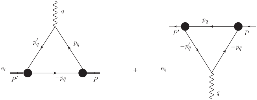
Figure 1: Diagrammatic representation of the pion electromagnetic form factor in one-loop approximation (cf Eq. (7)). The full dots represent the vertex functions for the initial and final bound states, respectively. Each vertex function, Eq. (6), contains the non perturbative dynamics and can be expressed in terms of the BS amplitude. The charge of the quark (anti-quark) is indicated by $e_{q(\bar{q})}$.

The covariant expression of the electromagnetic form factor. To evaluate the elastic em FF of the pion, it has been adopted the quantum-field formalism proposed by Mandelstam in Ref. [32], and originally applied to the deuteron. The leading idea was to take benefit of the prevalence of a bound-state pole in a suitable vacuum correlation function, where both the em current operator and the fermionic fields needed for extracting bound-state contributions (for initial and final two-body states) are present. Eventually, one is able to bring out the em current matrix elements between the relevant bound-states, obtaining an expression in terms of the pion BS amplitudes. Remarkably, the pion BS amplitude contains contributions not only from a two-fermion state, but also from an infinite set of states with two fermions and any number of gluons, that in the present study correspond to the infinite set of ladder exchanges necessary to reconstruct the bound-state pole.

By adopting the impulse approximation, i.e. a bare quark-photon vertex $i~{}\gamma^{\mu}$, the elastic em FF of a charged pion is pictorially represented á la Feynman in Fig. 1, by the sum of two triangle (one-loop) diagrams, weighted by the charge of the quark interacting with the virtual photon. Differently, the vertex between constituents and bound-system is a dressed one, described in terms of the BS amplitude by (see Fig. 1)

$${\cal V}(k,P)=S^{-1}(p_{q})~{}\Phi(k;P)~{}S^{-1}(p_{\bar{q}}),$$ (6)

where $p_{q}$ and $p_{\bar{q}}$ are the quark and anti-quark momenta, respectively, and $S^{-1}(p_{\bar{q}})=-i~{}(-/\!\!\!{p}_{\bar{q}}-m)$. In the case of a positive pion, within a $SU(2)$ framework, one has two contributions, where the virtual photon is absorbed by a $u$ quark or by a $\bar{d}$ one. Due to the underlying symmetries, both terms are equal (when taking the absolute value of the quark charge) so that the elastic FF is given by

$$F(Q^{2})=-i~{}{N_{c}\over M^{2}~{}(1+\tau)}\int\frac{d^{4}p_{\bar{q}}}{(2\pi)^{4}}~{}\text{Tr}\left[(-/\!\!\!{p}_{\bar{q}}-m)\bar{\Phi}(k^{\prime};P^{\prime})(/\!\!\!\!P+/\!\!\!\!P^{\prime})~{}\Phi(k;P)\right],$$ (7)

where $N_{c}$ is the number of colors, $\bar{\Phi}(k^{\prime};P^{\prime})$ is the BS-conjugated amplitude (see the explicit expression in Ref. [21]), $Q^{2}=-q^{2}=-(P^{\prime}-P)^{2}=-(p^{\prime}_{q}-p_{q})^{2}$, $(P+P^{\prime})^{2}=4M^{2}(1+\tau)$ with $\tau=Q^{2}/4M^{2}$ and the initial and final relative momenta are

$$k=\frac{P}{2}-p_{\bar{q}}=p_{q}-\frac{P}{2}~{}~{},\quad\quad k^{\prime}=\frac{P^{\prime}}{2}-p_{\bar{q}}=p^{\prime}_{q}-\frac{P^{\prime}}{2}=k+{q\over 2}.$$ (8)

For $q\to 0$, one has to obtain the charge normalization, $F(0)=1$, that in ladder approximation is equivalent to the BS normalization (see Ref. [21]).

By inserting the decomposition (3) and the NIR of the scalar functions $\phi_{i}(k;P)$ in Eq. (7), one gets

$$F(Q^{2})=~{}-i{N_{c}\over 4M^{2}~{}(1+\tau)}~{}\sum_{i,j=1}^{4}\int\frac{d^{4}k}{(2\pi)^{4}}\int_{0}^{\infty}d\gamma\int_{-1}^{1}dz\int_{0}^{\infty}d\gamma^{\prime}\int_{-1}^{1}dz^{\prime}~{}g_{j}(\gamma,z)g_{i}(\gamma^{\prime},z^{\prime})$$

$$\times~{}{\text{Tr}\Bigl{[}(/\!\!\!k-/\!\!\!\!P/2-m)~{}{\gamma^{0}~{}S_{j}^{\dagger}(k^{\prime};P^{\prime})~{}\gamma^{0}}(/\!\!\!\!{P}+/\!\!\!\!{P}^{\prime})~{}S_{i}(k;P)\Bigr{]}\over[\gamma+\kappa^{2}-k^{2}-(P\cdot k)z-i\epsilon]^{3}~{}~{}[\gamma^{\prime}+\kappa^{2}-k^{\prime 2}-(P^{\prime}\cdot k^{\prime})z^{\prime}-i\epsilon]^{3}}~{}~{},$$ (9)

After performing both traces and 4D integration, one gets the final expression for the elastic em FF, viz.

$$F(Q^{2})=\frac{N_{c}}{32\pi^{2}}\sum_{i,j=1}\int_{0}^{\infty}d\gamma\int_{-1}^{1}dz\int_{0}^{\infty}d\gamma^{\prime}\int_{-1}^{1}dz^{\prime}~{}g_{j}(\gamma,z)~{}g_{i}(\gamma^{\prime},z^{\prime})$$

$$\times~{}\int_{0}^{1}dy~{}y^{2}(1-y)^{2}~{}\frac{\tilde{c}_{ij}(y,\gamma,z;\gamma^{\prime},z^{\prime};Q^{2})}{\Bigl{[}\kappa^{2}+\gamma^{\prime}\,(1-y)+\gamma\,y+\alpha^{2}\,M^{2}\,+{Q^{2}\over 2}\,y\,(1+z)\,\beta\Bigr{]}^{4}}~{}~{},$$ (10)

where the coefficients $\tilde{c}_{ij}$, $\alpha$ and $\beta$ are given in A.

Besides the covariant expression, one could equivalently analyze the pion em FF within the LF framework, and obtain the so-called Drell-Yan expression of the elastic FF (see, e.g., Ref. [33]). As is well-known, within the LF framework, once a tiny mass is assigned to the exchanged boson, one can introduce a meaningful Fock-expansion of a bound-system state [33]. In particular, the valence wave function can be extracted from the BS amplitude through the LF projection onto the null-plane, $x^{+}=0$ (see Refs. [21, 23, 24, 25] for more details).

In the Drell-Yan frame ($q^{+}=0$), the em current operator component, $J^{+}=J^{0}+J^{3}$, is diagonal in the LF Fock-space [33], and one can profitably decompose the pion FF into two main contributions: (i) the LF valence contribution and (ii) the non valence one, generated by the higher Fock-components of the pion state, viz (see also Ref. [19])

$$F(Q^{2})=\sum_{n=2}^{\infty}F_{n}(Q^{2})=F_{\rm val}(Q^{2})+F_{\rm nval}(Q^{2})\,,$$ (11)

where $F_{n}(Q^{2})$ represents the contribution of the $n-$th Fock component of the pion state, $F_{\rm val}(Q^{2})=F_{n=2}(Q^{2})$ is the LF valence contribution normalized as $F_{\rm val}(0)=P_{\rm val}$, with $P_{\rm val}$ the valence probability (cf. Ref. [21]), and $F_{nval}(Q^{2})$ the non valence contribution with normalization $1-P_{\rm val}$. Hence, once we are able to compute both the full FF and the LF valence contribution, the non valence part can be obtained by using Eq. (11), so that the role of higher Fock-components in generating various features of the FF can be assessed, e.g., by evaluating the non valence contribution to the charge radius.

The LF valence contribution to the em form factor. The valence contribution to the FF is obtained from the matrix elements of the component $\gamma^{+}$ of the bare em current, between the initial and final LF valence states. In a Drell-Yan frame, where ${\bf P}_{\perp}+{\bf P}_{\perp}^{\prime}=0$, one obtains the following expression (see, e.g., Refs. [19, 24, 25, 34])

$$F_{\text{\rm val}}(Q^{2})=F^{S=0}_{\text{\rm val}}(Q^{2})+F^{S=1}_{\text{\rm val}}(Q^{2})=\frac{N_{c}}{16\pi^{3}}\int d{\mbox{\boldmath{$\kappa$}}}_{\perp}\int_{-1}^{1}dz\Bigl{[}\psi^{*}_{\uparrow\downarrow}(\gamma^{\prime},z)\psi_{\uparrow\downarrow}(\gamma,z)+\frac{{\mbox{\boldmath{$\kappa$}}}_{\perp}\cdot{\mbox{\boldmath{$\kappa$}}}^{\prime}_{\perp}}{\sqrt{\gamma\gamma^{\prime}}}\psi^{*}_{\uparrow\uparrow}(\gamma^{\prime},z)\psi_{\uparrow\uparrow}(\gamma,z)\Bigr{]}\,,$$ (12)

where $Q^{2}=|{\bf q}_{\perp}|^{2}$, $\gamma=|{\mbox{\boldmath{$\kappa$}}}_{\perp}|^{2}$, $\gamma^{\prime}=|{\mbox{\boldmath{$\kappa$}}}^{\prime}_{\perp}|^{2}$ and ${\mbox{\boldmath{$\kappa$}}}^{\prime}_{\perp}={\mbox{\boldmath{$\kappa$}}}_{\perp}+{1+z\over 2}~{}{\bf q}_{\perp}$. Notice that $z=(1-\xi)/2$ with the longitudinal-momentum fraction $\xi=p^{+}_{q}/P^{+}$, and hence for $z=-1$, i.e. $\xi=1$, the initial and final intrinsic momenta are collinear.

The two spin components $\psi_{\uparrow\downarrow}$ and $\psi_{\uparrow\uparrow}$, corresponding to the anti-aligned ($S=0$) and aligned ($S=1$) spin configurations, are proper integrals of the NWFs (see details in Ref. [21]).

In order to study the asymptotic behavior of the LF valence FF, we first observe that the rightmost contribution to Eq. (12) can be disregarded (checked also numerically) since (i) ${\mbox{\boldmath{$\kappa$}}}_{\perp}\cdot{\mbox{\boldmath{$\kappa$}}}^{\prime}_{\perp}$ vanishes for $\gamma\to 0$, precisely where the functions $\psi_{i}$ are bigger, and (ii) the overall weight of the $S=1$ configuration is smaller with respect to the $S=0$ one (cf. the calculated probabilities in Ref. [21]). Moreover, the fall-off of the $\psi_{\uparrow\downarrow}$ sets an effective range of $\gamma$ where the amplitudes yield sizable contributions. In conclusion, by disregarding the $S=1$ contribution and approximating $\psi_{\uparrow\downarrow}(\gamma^{\prime},z)\sim\psi_{\uparrow\downarrow}\left((1+z)^{2}Q^{2}/4,z\right)$ for large $Q^{2}$ one gets for the asymptotic em FF, namely $F^{(a)}_{val}(Q^{2})$,

$$F_{\text{\rm val}}(Q^{2})|_{Q^{2}\to\infty}\sim~{}{F^{(a)}_{\text{\rm val}}(Q^{2})=}\frac{N_{c}}{16\pi^{2}}\int_{-1}^{1}dz\,\psi_{\uparrow\downarrow}\left(\frac{(1+z)^{2}}{4}Q^{2},z\right)\,\int_{0}^{\infty}d\gamma\,\psi_{\uparrow\downarrow}(\gamma,z)\,,$$ (13)

where the last integral over $\psi_{\uparrow\downarrow}(\gamma,z)$ provides the corresponding distribution amplitude.

The asymptotic LF valence FF represents a physically motivated reference line for the valence FF, like the QCD asymptotic expression given in Ref. [26] does for the full FF. In particular, the asymptotic QCD FF, based on an asymptotic approximation of the anti-aligned spin component of the pion wave function, reads

$$Q^{2}F_{\text{asy}}(Q^{2})=8\pi\alpha_{s}(Q^{2})f^{2}_{\pi}\,,$$ (14)

where $\alpha_{s}(Q^{2})$ comes from [35] (notice that Eq. (4.4) of Ref. [26] has a different definition of $f_{\pi}$) and the decay constant is related to the anti-aligned component (see, e.g., Ref.[21]). A nice feature of the approximate formula in Eq. (13) is given by the possibility to understand that the integral in $z$ receives contributions, for large $Q^{2}$, from the region close to $z=-1$ ($\xi=1$), when we consider a quark ($z=1$, i.e. $\xi=0$ for an anti-quark), since the amplitude $\psi_{\uparrow\downarrow}(\gamma^{\prime},z)$ is sizable for small values of $\gamma^{\prime}=(1+z)^{2}~{}Q^{2}/4$. On the other hand, the amplitude is damped at the end-points, $z=\pm 1$. Therefore, from the competition of the two effects, one should expect that the integrand in $z$ of the total valence FF, Eq. (12), should be peaked close to $z=-1$ for large momentum transfers. This will be illustrated when presenting our numerical results.

Set	$m$	$B/m$	$\mu/m$	$\Lambda/m$	$P_{\rm val}$	$f_{\pi}$	$r_{\pi}$ (fm)	$r_{\rm val}$ (fm)	$r_{nval}$ (fm)
I	255	1.45	2.5	1.2	0.70	130	0.663	0.710	0.538
II	215	1.35	2	1	0.67	98	0.835	0.895	0.703

Table 1: The pion model, with $M=m_{\pi}=140$ MeV, for two parameter sets and the corresponding (i) valence probabilities $P_{\rm val}$, (ii) decay constants $f_{\pi}$ in MeV, (iii) pion charge radii, and (iv) their decomposition in valence and non-valence contributions (see Eq. (15)). The experimental values for the pion charge radius and $f_{\pi}$ are $r^{PDG}_{\pi}=0.659\pm 0.004$ fm, and $f^{PDG}_{\pi}=130.50(1)(3)(13)$ MeV, respectively (both from Ref. [35]).

Numerical results. The solutions of the coupled system for the NWFs were obtained after discretization that follows by expanding $g_{i}(\gamma,z)$ onto a bi-orthogonal basis, i.e. Laguerre polynomials for the non-compact variable, $\gamma$, and Gegenbauer polynomials for the compact one, $z$. In this way, one reduces the BSE into a generalized eigenvalue problem, where the squared coupling constant $g^{2}$ is the eigenvalue (see, e.g., Ref. [30]). As inputs, we have used the binding energy $B=2m-M$, the exchanged-boson mass, $\mu$, and the scale parameter, $\Lambda$, present in the extended quark-gluon vertex.

The adopted parameter sets, shown in Table 1, provide values of $f_{\pi}$ equal to $130$ and $98$ MeV, respectively (for a wider discussion and details, see Ref. [21]). Notice that: (i) the gluon mass $\mu$ is chosen as $637$ and $430$ MeV, with the first value suggested by LQCD results for the dressing function in the IR region, ranging in the interval 723-648 MeV in the Landau gauge [36]; (ii) the constituent quark mass $m$ is around 250 MeV, in order to be close to the IR values of the running mass in LQCD, varying in the interval 280-240 MeV [37] for momenta below $\sim 2\Lambda_{QCD}$; (iii) the parameter $\Lambda$ is taken of the order of $\Lambda_{QCD}$ [38, 39]. The set II is chosen for illustrating the crucial role of the correct reproduction of $f_{\pi}$, even with model parameters quite close to set I.

In Table 1, it is also shown the pion charge radius and its decomposition in valence and non valence contributions. It is observed that, in correspondence to the experimental value of the decay constant, $f_{\pi}=130$ MeV, we get $r_{\pi}=0.663$ fm, in fair agreement with the most recent PDG value, i.e. $r^{PDG}_{\pi}=0.659\pm 0.004$ fm  [35]. This is expected from the correlation between the two quantities (see Ref. [40]). The decomposition of the charge radius, that can yield valuable insights on the role of the higher Fock states, is straightforwardly obtained by using (i) the definition $r^{2}_{\pi}=-6~{}dF_{\pi}(Q^{2})/{dQ^{2}}\Bigr{|}_{Q^{2}=0}$, (ii) the decomposition given in Eq. (11) and (iii) the normalization of the valence and non valence em FFs. Explicitly, it reads

$$r^{2}_{\pi}=P_{\rm val}\,r^{2}_{\rm val}+(1-P_{\rm val})\,r^{2}_{nval}\quad\text{with}\quad P_{\rm val(nval)}\,r^{2}_{\rm val(nval)}=-6~{}dF_{\rm val(nval)}(Q^{2})/{dQ^{2}}\Bigr{|}_{Q^{2}=0}.$$ (15)

Table 1 illustrates that the higher Fock components generate a charge distribution more compact than the one from the LF valence wave function, i.e. $r_{\rm val}>r_{nval}$. The physical interpretation of this feature is quite natural, once we recall that the higher Fock components of the pion have larger virtualities, leading to very short lifetimes. Hence, there is no room for the quarks to fly too far from the pion center of mass.

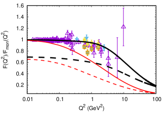
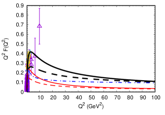
Figure 2: Left panel: Pion em form factor and its LF valence contribution, both divided by the monopole form factor $F_{mon}(Q^{2})=1/(1+Q^{2}/m_{\rho}^{2})$, vs $Q^{2}$. Thick solid line: covariant form factor obtained by using the parameter set I in Table 1, tuned to reproduce $f^{PDG}_{\pi}$. Thick dashed line: the LF valence contribution to the FF calculated with the set I (notice that $F_{\rm val}(0)=P_{\rm val}$). Thin lines: the same as the thick ones, but for the set II, shown for the sake of comparison. Experimental data correspond to: (i) Refs. [41, 42] (open upper triangle), (ii) Ref. [43] (filled upper triangle), (iii) Ref. [44] (filled lower triangle), (iv) Ref. [45] (open box) and (v) Ref. [46] (filled box). Right panel: the same as the left panel but with the em FF multiplied by $Q^{2}$, for illustrating the asymptotic behavior. Dot-dashed line: perturbative QCD prediction given by Eq. (14).

The pion em FF and its LF valence contribution divided by the monopole FF $F_{mon}(Q^{2})=1/(1+Q^{2}/m_{\rho}^{2})$ are presented in the left panel of Fig. 2 and compared with experimental data of Refs. [41, 42, 43, 44, 45, 46]. The thick lines correspond to the calculations performed by using the parameter set I. Let us recall that this set has been tuned in order to reproduce $f^{PDG}_{\pi}=130.50(1)(3)(13)$ MeV [35] and, consequently, getting the charge radius in agreement with $r^{PDG}_{\pi}$. The thin lines have been obtained by using the parameter set II, that has been chosen in order to have an insight of the effects on the FF when varying the decay constant (see Table 1).

The pion em FF is reproduced with a remarkable accuracy by the solution of the BSE obtained with the parameter set I. Moreover, the linear scale on the ordinate axis allows one to observe that for large enough momentum $F_{\rm nval}(Q^{2})$ becomes subleading and dominated by $F_{\rm val}(Q^{2})$, as expected. Within our dynamical model (for both sets) this valence dominance occurs above 80 GeV², where $F_{\rm val}(Q^{2})/F(Q^{2})$ starts to be $\geq~{}0.85$. In the right panel of Fig. 2, where a linear scale for the abscissa axis is adopted in order to emphasize the behavior of the FF at very large values of $Q^{2}$, the FF and its LF valence contribution multiplied by $Q^{2}$ are shown. Furthermore, for the sake of comparison, it is also presented the QCD asymptotic FF, $F_{asy}(Q^{2})$, given by Eq. (14) [26]. Our dynamical model becomes close to $F_{asy}(Q^{2})$ only around $Q^{2}\sim 100\,\rm{GeV^{2}}$, and it is consistent with the previous analysis of the valence dominance in the pion form factor [27].

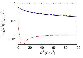
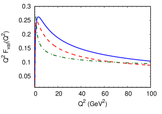
Figure 3: Left panel: anti-aligned (dashed line) and aligned (dot-dashed line) contributions to the valence FF vs $Q^{2}$ compared with the total LF valence FF (solid line). All three FF’s are divided by the monopole form factor. Right panel: asymptotic expression for the LF valence FF (dashed line), given in Eq. (13), compared to the valence FF (solid line), both multiplied by $Q^{2}$. Results presented for set I. Dot-dashed line: perturbative QCD prediction, Eq. (14).

Within the BSE approach, it is possible to evaluate even the contribution to the LF valence wave function from the two different spin configurations present in the pion (see details in Ref. [21]). This further decomposition of $F_{\rm val}$ is useful to illustrate the kinematical region where the purely relativistic aligned configuration (i.e. $S=1$) has interest. The anti-aligned and aligned contributions to $F_{\rm val}$ are shown in the left panel of Fig. 3. Noteworthy, at $Q^{2}=0$ the aligned contribution is quantitatively appreciable, since according to the probabilities of the $S=1$ and $S=0$ configurations [21] $F^{S=1}_{\rm val}(0)/F^{S=0}_{\rm val}(0)\sim 0.2$. For increasing $Q^{2}$ the ratio $F^{S}_{\rm val}/F_{\rm mon}$ quickly decreases, and $F^{S=1}_{\rm val}$ shows a dip below $Q^{2}=10~{}{\rm GeV^{2}}$. The zero in the aligned FF is due to the relativistic spin-orbit coupling that produces the term ${\mbox{\boldmath{$\kappa$}}}\cdot{\mbox{\boldmath{$\kappa$}}}^{\prime}$ in the FF (see Eq. (12)), which flips the sign of this contribution around $Q^{2}\sim 8\,\rm{GeV^{2}}$. In the right panel of Fig. 3, the approximate asymptotic expression for the valence FF given in Eq. (13) is compared to the valence FF and to the QCD prediction given by Eq. (14). The differences between the results obtained from the dynamical model are of the order of 20%, at large $Q^{2}$, while the full valence contribution is better approximated by the perturbative QCD result.

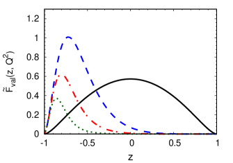
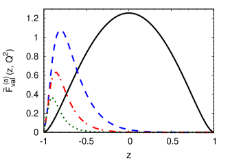
Figure 4: Left panel: $\tilde{F}_{\rm val}(z,Q^{2})$ vs $z$ and fixed values of $Q^{2}$. Solid line: $Q^{2}=0$. Dashed line: $Q^{2}=5~{}{\rm GeV^{2}}$. Dashed-dotted line: $Q^{2}=10~{}{\rm GeV^{2}}$. Dotted line: $Q^{2}=20~{}{\rm GeV^{2}}$. For the sake of visibility the results for $Q^{2}>0$ have been multiplied by a factor of 10. Right panel: the same as the left one, but for $\tilde{F}^{(a)}_{\rm val}(z,Q^{2})$, (cf. Eq. (13)). The results are presented for set I in both panels.

A 3D imaging of the pion charge distribution could be reached by a further analysis to be performed within our dynamical approach [15]. As a matter of fact, the covariant FF can be written in the $q^{+}=0$ frame as follows (see, e.g., Refs. [16, 17, 18]))

$$F(Q^{2})=\int_{-1}^{1}{dz\over 4\pi}\int{d{\bf b_{\perp}}\over(2\pi)^{2}}~{}e^{-i{\bf q}_{\perp}\cdot{\bf b}_{\perp}}~{}\rho_{ch}\Bigl{(}z,|{\bf b}_{\perp}|\Bigr{)}=\int_{-1}^{1}dz~{}\tilde{F}(z,Q^{2}),$$ (16)

where ${\bf b}_{\perp}$ is a vector in the impact parameter space, and $\rho_{ch}\Bigl{(}z,|{\bf b}_{\perp}|\Bigr{)}$ is the charge density and $\tilde{F}(z,Q^{2})$ a new quantity that we call sliced form factor. Noteworthy, such a quantity, for given $z$ and ${\bf b}_{\perp}$, is the no spin-flip generalized parton distribution with a vanishing skewness (see, e.g., Ref. [19]).

In the present work, we focus only on the valence component, leaving the sliced full FF and $\rho_{ch}\Bigl{(}z,|{\bf b}_{\perp}|\Bigr{)}$ to a detailed analysis in a future work. In Fig. 4, the $z$-dependence of the sliced valence FF is analyzed through two quantities: (i) $\tilde{F}_{\rm val}(z,Q^{2})$; and (ii) $\tilde{F}^{(a)}_{\rm val}(z,Q^{2})$, obtained from the asymptotic form given by Eq. (13). The analysis is done for $Q^{2}=0,~{}5,~{}10~{}\mbox{and}~{}20~{}{\rm GeV^{2}}$. In the left panel, the shape of $\tilde{F}_{\rm val}(z,Q^{2})$ supports the dominance of the end-point regions for large $Q^{2}$, as explained below Eq. (13). As a matter of fact, at $Q^{2}=0$ one has a symmetric behavior, while for increasing values of $Q^{2}$ the sliced FF’s sizably cumulates in the region close to $z=-1$ for a quark, as the $q\bar{q}$ pair is collinear to preserve the pion in the final state. Notice that the support of the bump shrinks as $\sim Q^{-2}$, which can be inferred by examining the approximate asymptotic formula given by Eq. (13).

Summary. We developed a fully four-dimensional treatment of the pion electromagnetic form factor based on the actual solution of the Bethe-Salpeter equation in Minkowski space. The ladder kernel is considered, as suggested by the suppression of the non-planar contributions for $N_{c}=3$ within the BS approach in a scalar QCD model [22]. The three inputs parameters, namely (i) the constituent mass, (ii) the gluon mass and (iii) the scale of the quark-gluon vertex, are inspired by the infrared properties of QCD, as obtained by LQCD. Once a fine tuning is carried out to reproduce the decay constant $f^{PDG}_{\pi}$, the obtained charge radius, $r_{\pi}=0.663~{}\text{fm}$, nicely agrees with the most recent experimental value, $r^{PDG}_{\pi}=0.659\pm 0.004~{}\text{fm}$ [35]. In correspondence, the predicted valence and non-valence radii amount to 0.71 fm and 0.54 fm, respectively. This means that the charge distribution generated by the $q\bar{q}$ pair in the higher Fock-components of the pion LF wave function is considerably more compact ($\sim$25%) than the valence configuration, although still significant. One should also keep in mind that the valence probability is about 70% and the remaining probability is associated with the occupancy of states with a $q\bar{q}$ pair and any number of gluons. The general behavior of the calculated em FF is illustrated in Fig. 2 and it is found to be in remarkable agreement with the existing data for $Q^{2}\leq 10~{}{\rm GeV^{2}}$. It is also interesting to notice that our covariant calculation matches the well-known perturbative QCD expression (14) for $Q^{2}>90~{}{\rm GeV^{2}}$, namely in the kinematical region where the valence contribution becomes dominant. Two further analyses have been presented, that allow a deeper understanding of the dynamics inside the pion. First, the decomposition of the valence component of the FF in terms of the spin configurations $S=0$, with about 75% of the valence probability, and $S=1$. The aligned spin configuration is a purely relativistic effect and has an impact at $Q^{2}=0$, counterintuitively (though understandable by the normalization constraint), but it becomes negligible at large $Q^{2}$. The second analysis is given by the study of the influence of the end-point behavior, i.e. the region close to $z=\pm 1$, on the valence FF at different values of the momentum transfer. Such an initial investigation could open a more stringent analysis of the charge distribution in the impact parameter space to explore the pion structure.

The unique features of Minkowski space methods applied to the continuum QCD approach are of great importance and need to be further explored. Future plans are to include (i) dressing functions for quark and gluon propagators (see Ref. [47], for an extension of the NIR framework to the fermion-photon coupled gap equations), and (ii) a more realistic quark-gluon vertex. The IR properties of the form factor that we have quantitatively explored within the Minkowski space approach might inspire further experimental works to disentangle valence and beyond-valence contributions.

Acknowledgments. J.H.A.N.  gratefully thanks Cédric Mezrag for helpful discussions. This study was financed in part by Conselho Nacional de Desenvolvimento Científico e Tecnológico (CNPq) under the grant 438562/2018-6 and 313236/2018-6 (WP), and 308486/2015-3 (TF), and by Coordenação de Aperfeiçoamento de Pessoal de Nível Superior (CAPES) under the grant 88881.309870/2018-01 (WP). J.H.A.N. acknowledges the support of the grants #2014/19094-8 from Fundação de Amparo à Pesquisa do Estado de São Paulo (FAPESP). E.Y. thanks for the financial support of the grants #2016/25143-7 and #2018/21758-2 from FAPESP. We thank the FAPESP Thematic Projects grants #13/26258-4 and #17/05660-0.

Appendix A Coefficients

The coefficients $\tilde{c}_{ij}$ in Eq. (Pion electromagnetic form factor with Minkowskian dynamics) are given by

$$\tilde{c}_{11}=\tilde{c}_{22}=-6\Bigl{(}\alpha+{1\over 2}\Bigr{)}~{},\quad\tilde{c}_{12}=\tilde{c}_{21}=6\frac{m}{M}~{},\quad\tilde{c}_{13}=\tilde{c}_{24}=-3{m\over M}~{}{Q^{2}\over M^{2}}~{}\beta~{},$$

$$\tilde{c}_{14}=\tilde{c}_{23}=3~{}{M^{2}_{\rm{cov}}\over M^{2}}-3~{}{Q^{2}\over 2M^{2}}~{}(2\alpha+1-4\beta)~{}\beta~{},\quad\tilde{c}_{31}=\tilde{c}_{42}=-3{m\over M}~{}{Q^{2}\over 2M^{2}}~{}(2\alpha+1-2\beta)~{},$$

$$\tilde{c}_{32}=\tilde{c}_{41}=3~{}{M^{2}_{\rm{cov}}\over M^{2}}+3{Q^{2}\over 4M^{2}}~{}\Bigl{[}(2\alpha+1)^{2}-12\beta\alpha+8\beta^{2}-6\beta\Bigr{]}~{},$$

$$\tilde{c}_{33}=\tilde{c}_{44}=-{M^{2}_{\rm{cov}}\over M^{2}}~{}(2\alpha+1)~{}\Bigl{(}{3\over 2}+{Q^{2}\over M^{2}}\Bigr{)}+3~{}{Q^{2}\over 2M^{2}}~{}\Bigl{(}1+{Q^{2}\over 4M^{2}}\Bigr{)}~{}(2\alpha+1)~{}(2\alpha+1-2\beta)\beta~{},$$

$$\tilde{c}_{34}=\tilde{c}_{43}=-{m\over M}~{}{M^{2}_{\rm{cov}}\over M^{2}}~{}\Bigl{(}3+{Q^{2}\over 2M^{2}}\Bigr{)}+3{m\over M}~{}{Q^{2}\over M^{2}}~{}\Bigl{(}1+{Q^{2}\over 4M^{2}}\Bigr{)}~{}~{}(2\alpha+1-2\beta)~{}\beta~{}~{}.$$ (17)

where $\alpha=[z\,y+z^{\prime}\,(1-y)]/2$ and $\beta=(1-y)~{}(1+z^{\prime})/2$.

References

- [1] T. Horn, C. D. Roberts, The pion: an enigma within the standard model, Journal of Physics G: Nuclear and Particle Physics 43 (7) (2016) 073001.
- [2] A. Accardi, et al., Electron Ion Collider: The Next QCD Frontier: Understanding the glue that binds us all, Eur. Phys. J. A 52 (9) (2016) 268. arXiv:1212.1701, doi:10.1140/epja/i2016-16268-9.
- [3] M. Oehm, C. Alexandrou, M. Constantinou, K. Jansen, G. Koutsou, B. Kostrzewa, F. Steffens, C. Urbach, S. Zafeiropoulos, and of the pion PDF from lattice QCD with dynamical quark flavors, Phys. Rev. D 99 (1) (2019) 014508. arXiv:1810.09743, doi:10.1103/PhysRevD.99.014508.
- [4] I. C. Cloët, C. D. Roberts, Explanation and Prediction of Observables using Continuum Strong QCD, Prog. Part. Nucl. Phys. 77 (2014) 1–69. arXiv:1310.2651, doi:10.1016/j.ppnp.2014.02.001.
- [5] G. Eichmann, H. Sanchis-Alepuz, R. Williams, R. Alkofer, C. S. Fischer, Baryons as relativistic three-quark bound states, Prog. Part. Nucl. Phys. 91 (2016) 1–100. arXiv:1606.09602, doi:10.1016/j.ppnp.2016.07.001.
- [6] C. Shi, I. C. Cloët, Intrinsic Transverse Motion of the Pion’s Valence Quarks, Phys. Rev. Lett. 122 (8) (2019) 082301. arXiv:1806.04799, doi:10.1103/PhysRevLett.122.082301.
- [7] K. D. Bednar, I. C. Cloët, P. C. Tandy, Distinguishing Quarks and Gluons in Pion and Kaon Parton Distribution Functions, Phys. Rev. Lett. 124 (4) (2020) 042002. arXiv:1811.12310, doi:10.1103/PhysRevLett.124.042002.
- [8] X. Ji, Parton Physics on a Euclidean Lattice, Phys. Rev. Lett. 110 (2013) 262002. arXiv:1305.1539, doi:10.1103/PhysRevLett.110.262002.
- [9] R. S. Sufian, C. Egerer, J. Karpie, R. G. Edwards, B. Joó, Y.-Q. Ma, K. Orginos, J.-W. Qiu, D. G. Richards, Pion Valence Quark Distribution from Current-Current Correlation in Lattice QCD, Phys. Rev. D 102 (5) (2020) 054508. arXiv:2001.04960, doi:10.1103/PhysRevD.102.054508.
- [10] G. C. Rossi, M. Testa, Note on lattice regularization and equal-time correlators for parton distribution functions, Phys. Rev. D 96 (1) (2017) 014507. arXiv:1706.04428, doi:10.1103/PhysRevD.96.014507.
- [11] A. Radyushkin, Quasi-parton distribution functions, momentum distributions, and pseudo-parton distribution functions, Phys. Rev. D 96 (3) (2017) 034025. arXiv:1705.01488, doi:10.1103/PhysRevD.96.034025.
- [12] L. Chang, I. Cloët, J. Cobos-Martinez, C. Roberts, S. Schmidt, P. Tandy, Imaging dynamical chiral symmetry breaking: pion wave function on the light front, Phys. Rev. Lett. 110 (13) (2013) 132001. arXiv:1301.0324, doi:10.1103/PhysRevLett.110.132001.
- [13] J. Carbonell, T. Frederico, V. Karmanov, Euclidean to minkowski bethe–salpeter amplitude and observables, The European Physical Journal C 77 (1) (2017) 58.
- [14] J. Lan, C. Mondal, S. Jia, X. Zhao, J. P. Vary, Parton Distribution Functions from a Light Front Hamiltonian and QCD Evolution for Light Mesons, Phys. Rev. Lett. 122 (17) (2019) 172001. arXiv:1901.11430, doi:10.1103/PhysRevLett.122.172001.
- [15] W. de Paula, E. Ydrefors, J. H. Alvarenga Nogueira, T. Frederico, G. Salmè, in preparation.
- [16] D. E. Soper, The Parton Model and the Bethe-Salpeter Wave Function, Phys. Rev. D 15 (1977) 1141. doi:10.1103/PhysRevD.15.1141.
- [17] S. J. Brodsky, G. F. de Teramond, Light-Front Dynamics and AdS/QCD Correspondence: The Pion Form Factor in the Space- and Time-Like Regions, Phys. Rev. D 77 (2008) 056007. arXiv:0707.3859, doi:10.1103/PhysRevD.77.056007.
- [18] G. A. Miller, Charge Density of the Neutron, Phys. Rev. Lett. 99 (2007) 112001. arXiv:0705.2409, doi:10.1103/PhysRevLett.99.112001.
- [19] T. Frederico, E. Pace, B. Pasquini, G. Salmè, Pion Generalized Parton Distributions with covariant and Light-front constituent quark models, Phys. Rev. D 80 (2009) 054021. arXiv:0907.5566, doi:10.1103/PhysRevD.80.054021.
- [20] L. Chang, I. Cloët, C. Roberts, S. Schmidt, P. Tandy, Pion electromagnetic form factor at spacelike momenta, Phys. Rev. Lett. 111 (14) (2013) 141802. arXiv:1307.0026, doi:10.1103/PhysRevLett.111.141802.
- [21] W. de Paula, E. Ydrefors, J. H. Alvarenga Nogueira, T. Frederico, G. Salmè, Observing the Minkowskian dynamics of the pion on the null-plane, Phys. Rev. D 103 (1) (2021) 014002. arXiv:2012.04973, doi:10.1103/PhysRevD.103.014002.
- [22] J. H. Alvarenga Nogueira, C.-R. Ji, E. Ydrefors, T. Frederico, Color-suppression of non-planar diagrams in bosonic bound states, Phys. Lett. B 777 (2018) 207–211. arXiv:1710.04398, doi:10.1016/j.physletb.2017.12.032.
- [23] T. Frederico, G. Salmè, M. Viviani, Two-body scattering states in Minkowski space and the Nakanishi integral representation onto the null plane, Phys. Rev. D 85 (2012) 036009. doi:10.1103/PhysRevD.85.036009.
- [24] J. H. O. Sales, T. Frederico, B. V. Carlson, P. U. Sauer, Renormalization of the ladder light front Bethe-Salpeter equation in the Yukawa model, Phys. Rev. C 63 (2001) 064003. doi:10.1103/PhysRevC.63.064003.
- [25] J. A. O. Marinho, T. Frederico, E. Pace, G. Salmè, P. Sauer, Light-front Ward-Takahashi Identity for Two-Fermion Systems, Phys. Rev. D 77 (2008) 116010. arXiv:0805.0707, doi:10.1103/PhysRevD.77.116010.
- [26] G. Lepage, S. J. Brodsky, Exclusive Processes in Quantum Chromodynamics: Evolution Equations for Hadronic Wave Functions and the Form-Factors of Mesons, Phys. Lett. B 87 (1979) 359–365. doi:10.1016/0370-2693(79)90554-9.
- [27] G. Lepage, S. J. Brodsky, Exclusive Processes in Perturbative Quantum Chromodynamics, Phys. Rev. D 22 (1980) 2157. doi:10.1103/PhysRevD.22.2157.
- [28] R. Abdul Khalek, et al., Science requirements and detector concepts for the electron-ion collider: EIC Yellow Report (2021). arXiv:2103.05419.
- [29] W. de Paula, T. Frederico, G. Salmè, M. Viviani, Advances in solving the two-fermion homogeneous Bethe-Salpeter equation in Minkowski space, Phys. Rev. D 94 (2016) 071901. doi:10.1103/PhysRevD.94.071901.
- [30] W. de Paula, T. Frederico, G. Salmè, M. Viviani, R. Pimentel, Fermionic bound states in Minkowski-space: Light-cone singularities and structure, Eur. Phys. Jou. C 77 (11) (2017) 764. arXiv:1707.06946, doi:10.1140/epjc/s10052-017-5351-2.
- [31] N. Nakanishi, Graph Theory and Feynman Integrals, Gordon and Breach, New York, 1971.
- [32] S. Mandelstam, Dynamical variables in the Bethe-Salpeter formalism, Proc. Roy. Soc. Lond. A 233 (1955) 248. doi:10.1098/rspa.1955.0261.
- [33] S. J. Brodsky, H.-C. Pauli, S. S. Pinsky, Quantum chromodynamics and other field theories on the light cone, Phys. Rept. 301 (1998) 299–486. arXiv:hep-ph/9705477, doi:10.1016/S0370-1573(97)00089-6.
- [34] C. Mezrag, H. Moutarde, J. Rodriguez-Quintero, From Bethe–Salpeter Wave functions to Generalised Parton Distributions, Few Body Syst. 57 (9) (2016) 729–772. arXiv:1602.07722, doi:10.1007/s00601-016-1119-8.
- [35] P. A. Zyla, et al., Review of Particle Physics, PTEP 2020 (8) (2020) 083C01. doi:10.1093/ptep/ptaa104.
- [36] O. Oliveira, P. Bicudo, Running Gluon Mass from Landau Gauge Lattice QCD Propagator, J. Phys. G 38 (2011) 045003. arXiv:1002.4151, doi:10.1088/0954-3899/38/4/045003.
- [37] M. B. Parappilly, P. O. Bowman, U. M. Heller, D. B. Leinweber, A. G. Williams, J. B. Zhang, Scaling behavior of quark propagator in full QCD, Phys. Rev. D 73 (2006) 054504. arXiv:hep-lat/0511007, doi:10.1103/PhysRevD.73.054504.
- [38] O. Oliveira, W. de Paula, T. Frederico, J. de Melo, The Quark-Gluon Vertex and the QCD Infrared Dynamics, Eur. Phys. J. C 79 (2) (2019) 116. arXiv:1807.10348, doi:10.1140/epjc/s10052-019-6617-7.
- [39] O. Oliveira, T. Frederico, W. de Paula, The soft-gluon limit and the infrared enhancement of the quark-gluon vertex, Eur. Phys. J. C 80 (5) (2020) 484. arXiv:2006.04982, doi:10.1140/epjc/s10052-020-8037-0.
- [40] R. Tarrach, Meson charge radii and quarks, Zeitschrift für Physik C Particles and Fields 2 (3) (1979) 221–223.
- [41] R. Baldini, S. Dubnička, P. Gauzzi, S. Pacetti, E. Pasqualucci, Y. Srivastava, Nucleon time-like form factors below the threshold, The European Physical Journal C-Particles and Fields 11 (4) (1999) 709–715.
- [42] R. Baldini, S. Dubnička, P. Gauzzi, S. Pacetti, E. Pasqualucci, Y. Srivastava, Determination of nucleon and pion form factors via dispersion relations, Nuclear Physics A 666 (2000) 38–43.
- [43] T. Horn, K. Aniol, J. Arrington, B. Barrett, E. Beise, H. Blok, W. Boeglin, E. Brash, H. Breuer, C. Chang, et al., Determination of the pion charge form factor at q 2= 1.60 and 2.45 (gev/c) 2, Physical review letters 97 (19) (2006) 192001.
- [44] G. Huber, H. Blok, T. Horn, E. Beise, D. Gaskell, D. Mack, V. Tadevosyan, J. Volmer, D. Abbott, K. Aniol, et al., Charged pion form factor between q 2= 0. 60 and 2. 45 gev 2. ii. determination of, and results for, the pion form factor, Physical Review C 78 (4) (2008) 045203.
- [45] V. Tadevosyan, H. Blok, G. Huber, D. Abbott, H. Anklin, C. Armstrong, J. Arrington, K. Assamagan, S. Avery, O. Baker, et al., Determination of the pion charge form factor for q 2= 0.60–1.60 gev 2, Physical Review C 75 (5) (2007) 055205.
- [46] J. Volmer, D. Abbott, H. Anklin, C. Armstrong, J. Arrington, K. Assamagan, S. Avery, O. Baker, H. Blok, C. Bochna, et al., Measurement of the charged pion electromagnetic form factor, Physical Review Letters 86 (9) (2001) 1713.
- [47] C. Mezrag, G. Salmè, Fermion and Photon gap-equations in Minkowski space within the Nakanishi Integral Representation method, Eur. Phys. J. C 81 (1) (2021) 34. arXiv:2006.15947, doi:10.1140/epjc/s10052-020-08806-x.