Abstract

Centrality measures are used in network science to evaluate the centrality of vertices or the position they occupy in a network. There are a large number of centrality measures according to some criterion. However, the generalizations of the most well-known centrality measures for weighted networks, degree centrality, closeness centrality, and betweenness centrality have solely assumed the edge weights to be constants. This paper proposes a methodology to generalize degree, closeness and betweenness centralities taking into account the variability of edge weights in the form of closed intervals (Interval-Weighted Networks – IWN). We apply our centrality measures approach to two real-world IWN. The first is a commuter network in mainland Portugal, between the 23 NUTS 3 Regions. The second focuses on annual merchandise trade between 28 European countries, from 2003 to 2015.

Keywords:  Centrality measures, Interval-Weighted Networks, Networks, Flow networks, Ford and Fulkerson algorithm

1 Introduction

The study of the centrality measures is one of the most important topics in network science (Borgatti, 2005; Brandes, 2008; Lu et al., 2016; Barabasi, 2016; Brandes et al., 2016; Ghalmane et al., 2019). One of the questions that naturally arise when analysing a network is: “Which are the central vertices in the network?” (Newman, 2018). The answer to this question depends on what we mean by important. Even though there is no general consensus on the exact definition of “importance”, in a structural approach, which is the most common, the importance of a vertex is usually related to the concept of being the most connected vertex or being positioned in the center of the network (Freeman, 1977, 1979; Bonacich, 1987; Borgatti and Everett, 2006). Essentially, a vertex positioned in the center of a network has advantages over other vertices, as it is directly linked to many other vertices (has more edges) or acts as an intermediary in communicating with other vertices, either at speed (it is closer) or in the flow control with which it reaches the other vertices (it is between). Identifying these “vital” vertices allow us to control the outbreak of epidemics, to conduct advertisements for e-commercial products, to predict popular scientific publications, and so on (Lu et al., 2016). There are a large number of centrality measures that capture the varying importance of the vertices (vertex-level measures) in a network according to some criterion, such as reachability, influence, embeddedness, control the flow of information (Rodrigues, 2019). Some of these most well known measures are degree centrality and closeness centrality (Sabidussi, 1966; Freeman, 1979), Betweeness centrality (Freeman, 1977), and Eigenvector centrality (Bonacich, 1972) along with its variants (Bonacich, 1987) and Page rank (Brin and Page, 1998). Other centrality measures are Katz centrality (Katz, 1953), Information centrality (or S-Z centrality index) (Stephenson and Zelen, 1989), Betweeness centrality based on flow networks (Freeman et al., 1991), Valente and Foreman (1998) integration and radiality measures, Centrality based on game theory (Gómez et al., 2003), Betweeness centrality based on random walks (Newman, 2005), among others.

Recently, Gómez et al. (2013) introduced a centrality measure based on bi-criteria network flow. Martin et al. (2014) proposed a new centrality measure based on the leading eigenvector of the Hashimoto or nonbacktracking matrix. Du et al. (2014) presented TOPIS as a new measure of centrality. Lu et al. (2016) suggested a novel measure of node influence based on comprehensive use of the degree method, H-index and coreness metrics. Brandes et al. (2016) propose a variant notion of distance that maintains the duality of closeness-as-independence with betweenness also on valued relations. Qiao et al. (2017) introduced a novel entropy centrality approach. Wu et al. (2019) introduced eigenvector multicentrality based in a tensor-based framework. Ghalmane et al. (2019) extended all the standard centrality measures defined for networks with no community structure to modular networks Modular centrality. Zhang et al. (2020) derive a new centrality index resilience centrality. A comprehensive explanation of some of these measures can be found in Lu et al. (2016) and the book by Newman (2018).

In this paper, we focus only on the most influential and well-known centrality measures, degree, closeness and betweenness Freeman (1979). Initially these three measures were formalized for binary (unweighted) networks. However, as Freeman (1979) refers, binary representations fail to capture any of the important variability in strength, and naturally these measures were later extended to weighted networks. Firstly, by allowing to capture the strength of an edge focusing only on edge weights (Newman, 2001; Brandes, 2001; Barrat et al., 2004). Secondly by taking into consideration both the weight and the number of edges including a tuning parameter, $\alpha$ (Opsahl et al., 2010). Moreover, as some centrality measures (closeness and betweenness) are based on the shortest paths, they do not take into account the flow of the edge content along non-shortest paths. Thus, Freeman et al. (1991) proposed a betweenness measure based on Ford and Fulkerson’s (FF) model of network flows (Ford and Fulkerson, 1956, 1957, 1962), thereby allowing to account for the flow of the edges of the entire network.

Nevertheless, none of the above methodologies allows accounting for the variability observed in the original data. The main contribution of this paper is the development of three new measures for degree, closeness and betweenness, taking into account the networks’ variability of edge weights in the form of closed intervals. This way, a closed interval may be used to model the precise information of an objective entity that comprehends intrinsic variability (ontic view), i.e., an interval $A$ is a value of a set-valued variable $X$, so we can write $X=A$ (Couso and Dubois, 2014; Grzegorzewski and Śpiewak, 2017). We call such networks interval-weighted networks (IWN) (see Figure 2), and consequently, we name these measures the interval-weighted degree (IWD), interval-weighted flow betweenness (IWFB) and interval-weighted flow closeness (IWFC). Our methodology is depicted in Figure 1. The dashed lines indicate the methods followed in this paper in the generalization of the centrality measures for interval-weighted networks.

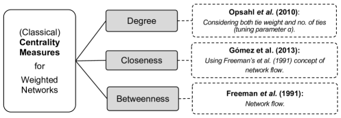
Figure 1: Scheme of the generalizations made for interval-weighted networks (IWN) of the three (classical) measures of vertex centrality, degree, closeness and betweenness. In dashed lines are indicated the approaches adopted when generalizing to IWN.

The remaining of the paper is organized as follows. We start by briefly introducing the basic terms and concepts of interval arithmetic and interval order relations and we propose a new order relation between intervals (Section 2). Then, in Section 3 we recall the centrality measures for weighted networks. First, we present the degree for the general case and also taking into account both edge weights and the number of edges introducing a tuning parameter $(\alpha)$. Second, we define the concept of flow networks for the case of an (undirected) interval-weighted network and corresponding centrality measures, flow closeness and flow betweenness. In Section 4, we generalize degree, flow betweenness and flow closeness to the case of interval-weighted networks. In Section 5, we apply our generalizations of degree, flow betweenness and flow closeness to the case of interval-weighted networks in two real-world applications. Finally, in Section 6 we conclude and discuss the outcomes obtained with our methodology.

2 Interval Analysis

Let $\underline{x},\overline{x}\in\mathbb{R}$ such that $\underline{x}\leqslant\overline{x}$. An interval number $[\underline{x},\overline{x}]$ is a closed bounded nonempty real interval, given by $[\underline{x},\overline{x}]=\{x\in\mathbb{R}\colon\underline{x}\leqslant x\leqslant\overline{x}\}$, where $\underline{x}=\min([\underline{x},\overline{x}])$ and $\overline{x}=\max([\underline{x},\overline{x}])$ are called, respectively, the lower and upper bounds (endpoints) of $[\underline{x},\overline{x}]$. The set $[\mathbb{R}]$ of interval numbers is a subset of the powerset of $\mathbb{R}$ such that $[\mathbb{R}]=\big{\{}X\in\wp\,(\mathbb{R})\colon(\exists\underline{x}\in\mathbb{R})\,(\exists\overline{x}\in\mathbb{R})\,(X=[\underline{x},\overline{x}])\big{\}}.$ Since, corresponding to each pair of real constants $\underline{x},\overline{x}\ (\underline{x}\leqslant\overline{x})$ there exists a closed interval $[\underline{x},\overline{x}]$, the set of interval numbers is infinite. We say that $X$ is degenerate if $\underline{x}=\overline{x}$. By convention, a degenerate interval $[x,x]$ is identified with the real number $x$ (e.g., $1=[1,1]$). For any two intervals $X=[\underline{x},\overline{x}]$ and $Y=[\underline{y},\overline{y}]$, in terms of the intervals’ endpoints, the four classical operations of real arithmetic can be extended to intervals as follows (Moore et al., 2009):

• Interval addition, $X+Y=[\underline{x},\overline{x}]+[\underline{y},\overline{y}]=[\underline{x}+\underline{y},\overline{x}+\overline{y}]$;

• Interval multiplication, $X\cdot Y=[\underline{x},\overline{x}]\cdot[\underline{y},\overline{y}]=\big{[}\min\{\underline{x}\underline{y},\underline{x}\overline{y},\overline{x}\underline{y},\overline{x}\overline{y}\},\max\{\underline{x}\underline{y},\underline{x}\overline{y},\overline{x}\underline{y},\overline{x}\overline{y}\}\big{]}$;

• Interval subtraction, $X-Y=X+(-Y)$ where $-Y=[-\overline{y},-\underline{y}]$ (reversal of endpoints).

• Interval division for any $X\in\mathbb{R}$ and any $Y\in[\mathbb{R}]_{\widetilde{0}}$, is defined by $X\div Y=X\cdot(Y^{-1})$, where $Y^{-1}=1/Y=[1/\overline{y},1/\underline{y}]$, assuming that $0\not\in Y$.

Intervals can also be represented by their midpoint (or mean, or center) $m$ and half-width (or radius), $rad$. So, $X=\interval{\underline{x}}{\overline{x}}=\langle m(X),rad(X)\rangle$, where $m(X)=\mfrac{(\underline{x}+\overline{x})}{2}$ and $rad(X)=\mfrac{(\overline{x}-\underline{x})}{2}$.

The infimum between two intervals $X=\interval{\underline{x}}{\overline{x}}$ and $Y=\interval{\underline{y}}{\overline{y}}$ is defined to be $\inf(X,Y)=[\inf(\underline{x},\underline{y}),\inf(\overline{x},\overline{y})]$. Similarly, the supremum between two intervals $X=\interval{\underline{x}}{\overline{x}}$ and $Y=\interval{\underline{y}}{\overline{y}}$ is defined to be $\sup(X,Y)=[\sup(\underline{x},\underline{y}),\sup(\overline{x},\overline{y})]$ (Dawood, 2011). An operation whose operands are intervals $(\interval{\underline{x}}{\overline{x}})$, and whose result is a point interval (or a real number) is called a point interval operation, such as the: infimum $\inf(\interval{\underline{x}}{\overline{x}})=\min(\interval{\underline{x}}{\overline{x}})=\underline{x}$ and supremum $\sup(\interval{\underline{x}}{\overline{x}})=\max(\interval{\underline{x}}{\overline{x}})=\overline{x}$. Finally, another important definition of a point interval operation is the Hausdorff distance (or metric) between two intervals (see, e.g., Billard and Diday, 2007): $d(X,Y)=d(\interval{\underline{x}}{\overline{x}},\interval{\underline{y}}{\overline{y}})=\max\{|\underline{x}-\underline{y}|,|\overline{x}-\overline{y}|\}$.

Interval arithmetic pitfalls:

Useful properties of ordinary real arithmetic fail to hold in classical interval arithmetic. Some of the main disadvantages of the classical interval theory are (Dawood, 2011): (i) Interval dependency – subtraction and division are not the inverse operations of addition and multiplication, respectively; (ii) Distributive law does not hold – only a subdistributive law is valid – $\forall X,Y,Z\in[\mathbb{R}]\ Z\times(X+Y)\subseteq Z\times X+Z\times Y$.

2.1 Interval order relation

Till date one main dilemma in using interval data for decision problems is perhaps the choice of an appropriate interval order relation. Unlike real numbers that are ordered by a strict transitive relation “$<$” (if $a<b$ and $b<c$, then $a<c$ for any $a,b$, and $c\in\mathbb{R}$), the ranking of intervals is not symmetric, and as consequence, in many situations, the definitions cannot differentiate two intervals in general, even though they can be applied efficiently to solve the prescribed models (Karmakar and Bhunia, 2014). As a consequence, theoretically, intervals can only be partially ordered in $[\mathbb{R}]$. According to Moore et al. (2009), two transitive order relations can be defined for intervals: (i) $X<Y\Leftrightarrow\overline{x}<\underline{y}$, and (ii) $X\subseteq Y\Leftrightarrow\underline{y}\leqslant\underline{x}\ \text{and}\ \overline{x}\leqslant\overline{y}$ (set inclusion). Nevertheless, when a choice has to be made among alternatives, the comparison is indeed needed. There are several different approaches in the literature for ordering intervals (Hu and Wang, 2006; Sengupta and Pal, 2009; Guerra and Stefanini, 2012; Stefanini et al., 2019). A detailed description and comparison between these and other ranking definitions is given in (Karmakar and Bhunia, 2012).

Bearing in mind the above definitions, and according to Hossain’s methodology (Hossain, 2009), we may define the following order relation:

Definition 2.1.

Given two intervals $X,Y\in\mathbb{R}$, $X\leqslant Y$, iff $m(X)\leqslant m(Y)$. Furthermore $X<Y$ iff $X\leqslant Y$ and $X\neq Y$. In the case where the midpoints of $X$ and $Y$ coincide $m(X)=m(Y)$, the intervals $X$ and $Y$ are said to be equivalent $X\approx Y$. We propose the following order relation: $X\leqslant Y$ is determined by choosing the interval that captures the “maximum variability” between the two intervals, i.e., the interval with the highest radius. For example, if $m(X)=m(Y)$ the decision for $X\leqslant Y$ implies that $rad(Y)>rad(X)$.

To exemplify and illustrate the applicability of these definitions in a simple network, we built three scenarios for ranking a pair of intervals. The results are shown in Table 1.

Table 1: Interval ordering for the order relation “$\leqslant$”, to choose the “greater interval”.

Interval relations Order relation “$\leqslant$” Type of interval Non-overlapping Partially overlapping Completely overlapping: $m(X)=m(Y)$ $X\cap Y$ $X\cap Y=\varnothing$ $X\cap Y\neq\varnothing$ $X\cap Y\neq\varnothing\land X\subseteq Y$ $d_{H}(X,Y)$ $\max(|{-3}|,|{-3}|)=3$ $\max(|{-2}|,|{-2}|)=2$ $\max(|{1}|,|{-1}|)=1$ $\inf(X,Y)$ $\min([1,3],[4,6])=[1,3]$ $\min([1,4],[3,6])=[1,4]$ $\min([2,5],[1,6])=[1,5]$ $\sup(X,Y)$ $\max([1,3],[4,6])=[4,6]$ $\max([1,4],[3,6])=[3,6]$ $\max([2,5],[1,6])=[2,6]$ $\langle midpoint,\operatorname{half-width}\rangle$ $X=\langle 2,1\rangle;Y=\langle 5,1\rangle$ $X=\langle 2.5,1.5\rangle;Y=\langle 4.5,1.5\rangle$ $X=\langle 3.5,1.5\rangle;Y=\langle 3.5,2.5\rangle$ Decision = choose the greater interval $choose\ Y$ $choose\ Y$ $choose\ Y$

3 Centrality measures for weighted networks: degree; flow betweenness and flow closeness

Degree centrality

of a vertex $i$ for weighted networks (or the vertex strength) is defined as the sum of weights attached to edges connected to vertex $i$ (Barrat et al., 2004). Usually it is formalized as:

$$s_{i}=C^{W}_{D}(i)=\sum^{n}_{j=1}w_{ij}\qquad s_{i}>0$$ (1)

where $w_{ij}$ is the entry of the $i$th row and $j$th column of the weighted adjacency matrix $W$.
Opsahl et al. (2010) include a tuning parameter, $\alpha$, to address the relative importance of the number of edges compared to edge weights associated with a vertex $i$, this is formalized as:

$$C^{W\alpha}_{D}(i)=k_{i}{\left(\frac{s_{i}}{k_{i}}\right)}^{\alpha}=k^{(1-\alpha)}_{i}s^{\alpha}_{i}$$ (2)

where $k_{i}$ is the number of vertices that a focal vertex $i$ is connected to.

Briefly, when $0<\alpha<1$, both vertex degree and strength will be taken into account, when $\alpha>1$, the measure would positively value edge strength and negatively value the number of edges, for $\alpha=0$, the measure is solely based on the number of edges, and for $\alpha=1$ the measure is based only on edge weights (see Opsahl et al. 2010 for details).

Garas et al. (2012) exemplifies the situation described above, through economic or commercial networks where weights generally play an important role (usually representing the flow of capital or the flow of trade). In these cases, the focus is usually on the vertices with higher strength, usually the most important. Thus, in such networks the presence of vertices with a high degree and relatively small strength can influence the results obtained by methods that are based only on the degree.

Flows in undirected weighted networks

The reason why we opted for using Freeman’s (Freeman et al., 1991) approach of flow networks to generalize both betweenness (Freeman, 1979; Opsahl et al., 2010) and closeness (Newman, 2001; Brandes, 2001; Opsahl et al., 2010) to weighted networks, was mainly because, first Freeman et al. (1991) and later Newman (2005), Brandes and Fleischer (2005) and Borgatti (2005), pointed out that closeness and betweenness centrality measures based on the shortest paths do not take into account the flow of the edge content (e.g., information) along non-shortest paths, assuming that the edge content only flows along the shortest possible paths (Borgatti, 2005). Therefore, these measures are unlikely to characterize human communication, disease proliferation, etc. (Barbosa et al., 2018). To contour this, Freeman et al. (1991) proposed a betweenness measure based on Ford and Fulkerson’s (FF) model of network flows (Ford and Fulkerson, 1956, 1957, 1962).

Note 3.1.

Since both the flow networks and the Ford and Fulkerson algorithm (Ford and Fulkerson, 1962) have been defined for direct networks, it is first necessary to transform an undirect network into a direct network; this is done as follows: for an undirected and connected network $G=(V,E)$, where $V\neq\emptyset$ is a finite set of vertices and $E$ is a set of pairs of vertices called edges $E\subseteq\big{\{}(i,j)\colon i,j\in V\big{\}}$, the extension of Ford and Fulkerson algorithm (Ford and Fulkerson, 1962) is done by considering two direct edges $(i,j)$ and $(j,i)$ (hereinafter $\{i,j\}$), one in each direction, for each edge in the original network. Considering the two direct edges between a given pair of vertices, when an edge is used in a flow, the other edge cannot be used (Freeman et al., 1991; Schroeder et al., 2004; Gómez et al., 2013).

Definition 3.1 (Undirected Flow Network).

Given a connected undirected network $G=(V,E)$, and a pair of vertices $s$ (source), and $t$ (sink) $\in V$, let $f(i,j)$ be the flow in the edge $(i,j)\in E$, and let the maximum allowable flow on that edge be $c(i,j)$, its capacity $(c\colon E\rightarrow\mathbb{R^{+}})$. A flow in $G$ is a function $f\colon V\times V\rightarrow\mathbb{R}$ that satisfies the following properties:

• capacity constraint – the resources used by a flow on an edge cannot be greater than the capacity of that edge: $0\leqslant f(i,j)\leqslant c\left(\{i,j\}\right),\ \forall i,j\in V$;

• skew symmetry – the network flow from vertex $i$ to $j$ is the negative of the network flow in the reverse direction: $f(i,j)=-f(j,i),\ \forall i,j\in V$ (and thus, $f(i,i)=-f(i,i)=0$);

• flow conservation – the sum of all flows that enter in a vertex (negative flows) plus the sum of all flows that leave that vertex (positive flows) is null: $\sum_{j\in V}f(i,j)=0,\forall i\in V-\{s,t\}$.

Thus, the value of a flow is the sum of all outgoing flow $f(i,j)$ from the source $s$, defined as: $|f|=\sum_{j\in V}f(s,j)=\sum_{j\in V}f(j,t)$.

However, we are interested in finding the overall flow between pairs of vertices along all the paths that connect them. To find out the maximum allowable flow (hereafter, max-flow) on a flow network from any source $i$ to any sink $j$, we will use the algorithm developed by Ford and Fulkerson (1962). This algorithm uses flow-augmenting paths to increase existing flows in the network, so that in each iteration the flow is greater. The basic idea behind the FF algorithm for undirected networks, is as follows:

Definition 3.2 (Ford and Fulkerson algorithm).

Given a connected network $G=(V,E)$, where $V$ is a set of vertices and $E$ is a set of edges between these vertices $(E\subseteq\{\{i,j\}:i,j\in V\})$ , for a flow $f$ between a pair of vertices $(i,j)$, the forward residual capacity from $i$ to $j$ is denoted by $c_{f}(i,j)=c\left(\{i,j\}\right)-f(i,j)$, where $c\left(\{i,j\}\right)$ is the forward capacity of $(i,j)$ (the order of vertices connected by an edge does not matter, as well as the associated capacity).

The residual network is basically an auxiliary network used by the algorithm, defined as: given a network $G=(V,E)$, let $f$ be a flow in $G$, the residual network induced by $f$ is a network $G_{f}=(V,E_{f})$, where $E_{f}=\{(i,j)\in V\times V\colon c_{f}(i,j)>0\}$. The residual network is always directed, either for directed or undirected networks. The residual capacity from $j$ to $i$, in the backward direction of the edge $(i,j)$, is defined as $c_{f}(j,i)=c\left(\{j,i\}\right)+f(i,j)$. That is, the residual capacity is the additional flow one can send on an edge, possibly by cancelling some flow in opposite direction.

Let $p$ be a path from $s$ to $t$ that is allowed to transverse edges in either the forward or backward direction, the residual capacity $c_{f}(p)$ of a path $p$ is the minimum residual capacity of its edges, that is, $c_{f}(p)=\min\limits_{(i,j)\in p}c_{f}(i,j)$. If $c_{f}(p)>0$, then $p$ is called an augmented path. A value of total flow can be increased by adding the minimum capacity on each forward edge and subtracting it from every backward edge in the augmented path.

By repeating this process of finding the augmented paths on a flow network, the total flow can be increased to the maximum within capacity constraints.

The pseudo-code bellow (see Algorithm 1) describes the Ford & Fulkerson algorithm for undirected networks (Schroeder et al., 2004).

Algorithm 1 Pseudo-code: Ford and Fulkerson algorithm for undirected networks

Input: A connected undirected flow network $G=(V,E)$
Output: The maximum flow $f$ on $G$

1. for each edge $\{i,j\}\in E$ do

2. $\qquad f[i,j]\leftarrow 0$

3. $\qquad f[j,i]\leftarrow 0$

4. while there exists a path $p$ from $s$ to $t$ with no cycles in the residual network $G_{f}$ do

5. $\qquad\Delta\leftarrow\min\{c_{f}(i,j)\colon(i,j)\in p\}$

6.        for each edge $(i,j)$ in $p$ do

7. $\qquad\qquad f[i,j]\leftarrow f[i,j]+\Delta$

8. $\qquad\qquad f[j,i]\leftarrow-f[i,j]$

9. return $f$

Having defined a flow network (Definition 3.1) and the FF max-flow algorithm (Definition 3.2), next we present the respective flow centrality measures.

Note 3.2.

All the generalizations take into account only undirected and connected weighted networks, $G=(V,E)$, where $V\neq\emptyset$ is a finite set of vertices and $E$ is a set of positive weighted edges, where the weights measure the strength $w_{ij}\geqslant 0$, $E\subseteq\big{\{}(i,j)\colon i,j\in V\big{\}}$. For unweighted networks, we define $w_{ij}=1$ if there is an edge between vertices $i$ and $j$ and zero otherwise.

Flow betweenness $FB(i)$ – is defined as the degree to which the maximum flow between all unordered pairs of vertices depends on an intermediary vertex $i$. Thus, the flow betweenness $FB(i)$ is defined as (Freeman et al., 1991):

$$FB(i)=C^{W}_{FB}(i)=\sum^{n}\limits_{\begin{subarray}{c}{j=1}\\ j\neq i\end{subarray}}\sum^{n}\limits_{\begin{subarray}{c}{k=1}\\ k\neq{i,j}\end{subarray}}f_{jk}(i),\leavevmode\nobreak\$$ (3)

where $f_{jk}(i)$ is the maximum flow from $j$ to $k$ that passes through vertex $i$.

Flow closeness $FC(i)$ – although Freeman et al. (1991) did not formally define flow closeness as a centrality measure, we can partially extend this as the maximum flow between one vertex $i$ and the rest of the network, as:

$$FC(i)=C^{W}_{FC}(i)=\sum^{n}_{j=1}f_{ij},$$ (4)

where $f_{ij}$ represents the maximum flow from vertex $i$ to vertex $j$. It is important to highlight that this measure has a poor ability to distinguish which are the vertex(ices) closest to every other vertices when in presence of special situations, such as when the network has a star topology (one central vertex – hub – and the remaining $n-1$ vertices connected to it) in which all links have the same strength (Gómez et al., 2013).

4 Centrality Measures for Interval-Weighted Networks

In classical network flow theory, a capacity $c(i,j)$ is associated with each edge between vertex vertex $i$ and $j$, denoting the maximum amount that can flow on the edge and a lower bound $l(i,j)$ representing the minimum amount that must flow on the edge (Ahuja et al., 1993). Nevertheless, the maximum flow problem is restricted by flow bounds considering only the maximum flow capacity $c(i,j)$ of an edge between each pair of vertices $i$ and $j$, thus assuming that this capacity is constant. However, in real-world applications, these capacities may vary within ranges rather than being constants (Ahuja et al., 1993). To better model such variability on an edge, instead of using constants, we represent flow capacities as intervals (Hu and Hu, 2008; Sengupta and Pal, 2009; Hossain and Gatev, 2010; Hossain, 2009; Bozhenyuk et al., 2017). An interval representation of these capacities allows taking into account the variability observed in the original network, thereby minimizing the loss of information. In what follows, we extend the degree, flow betweenness and flow closeness centrality measures to the general case of interval-weighted networks. First, we introduce the Interval-Weighted Degree (IWD), extending Opsahl et al. (2010) concept of a tuning parameter to give relevance to both edge weights and number of edges attached to a vertex. Secondly, based on capacity flow networks, using FF max-flow algorithm (Ford and Fulkerson, 1962), we present the Interval-Weighted Flow Closeness (IWFC) and Interval-Weighted Flow Betweenness (IWFB).

Conversion of an interval-weighted undirected network into its corresponding direct version

Before generalizing the centrality measures discussed in Section 3 to IWN, as mentioned in Note 3.1, it is first necessary to transform an undirected interval-weighted network into a direct one. Figure 2 shows an undirected interval-weighted network and its transformation into a directed interval-weighted network (for the sake of simplicity, in future representations of IWN, only one undirected interval-weighted edge will be represented, as shown in Figure 2.a).

(a)

(b)

Figure 2: (a) Undirected Interval–Weighted Network, and its corresponding (b) Directed Interval–Weighted Network (Schroeder et al., 2004).

Flows in undirected interval-weighted networks

The generalization to interval-weighted networks (IWN) of Freeman’s betweenness and closeness centrality measures (Freeman et al., 1991), according to the methodology based on “flow networks” discussed in Section 3, faced two major drawbacks proper of interval arithmetic (Moore et al., 2009):

• firstly, because of the non-existence of inverse elements. The generalization of closeness and betweenness to weighted networks done by Newman (2001) and Brandes (2001), respectively, inverted the edge weights to consider them as costs and then applied the Dijkstra’s (1959) shortest path algorithm (the least costly path connecting to vertices was the shortest path between them). Thus, the identification and length of the shortest paths is based on the sum of the inverted edge weights and is defined as: $d^{W}(i,j)=\min\left(\frac{1}{w_{ih}}+\dots+\frac{1}{w_{h^{\prime}j}}\right)$, where $h$ and $h^{\prime}$ are intermediary vertices on paths between vertices $i$ and $j$;

• secondly, to what is known as interval dependency problem. The use of flow capacities as intervals raises some difficulties when calculating the shift of a flow on an augmented path, since the real number arithmetic property of additive inverse (i.e., if $b=c-a$, then $a+b=c$) is not valid for interval subtraction, e.g., $[1,5]+[1,3]=[2,8]$, but $[2,8]-[1,3]=[-1,7]\neq[1,5]$ (see section 2 for a detailed explanation about interval arithmetic).

Lexicographic order

To circumvent the above mentioned difficulty, the lexicographic order was used to prove that the maximum flow is obtained with the maximum flow values at each edge, and the minimum flow with the minimum flow values at each edge (see Appendix A for details).

4.1 Interval-Weighted Degree (IWD)

The extension of the degree to the case of an interval-weighted network is done first by considering only the vertices strength, i.e., the sum of the edge interval-weights (Barrat et al., 2004), and secondly by taking into consideration both the number of edges and the edges strength by introducing a tuning parameter $\alpha$ (Opsahl et al., 2010). The following definitions express these concepts:

Definition 4.1.

Using (1) and (2), the generalization of degree to an IWN is formalized as:

$$IWD(i)=s^{IW}_{i}=C^{IW}_{D}(i)=\sum^{n}_{j=1}\left[\underline{w}_{ij},\overline{w}_{ij}\right],$$ (5)

where $\left[\underline{w}_{ij},\overline{w}_{ij}\right]$ are the interval–weights $(\overline{w}_{ij}\geqslant\underline{w}_{ij}>0)$.

Definition 4.2.

The generalization of Opsahl et al. (2010) approach, which consists in the inclusion of a tuning parameter, $\alpha$, to address the relative importance of the number of edges compared to edge interval-weights, is formalized as:

$$IWD^{\alpha}(i)=C^{IW\alpha}_{D}(i)=k^{(1-\alpha)}_{i}\left(\sum^{n}_{j=1}\left[\underline{w}_{ij},\overline{w}_{ij}\right]\right)^{\alpha}=k^{(1-\alpha)}_{i}\left(s^{IW}_{i}\right)^{\alpha}.$$ (6)

where $k_{i}$ is the number of vertices that a focal vertex $i$ is connected to.

The following is an example of our approach to degree in an IWN.

Example 4.1 (Interval-Weighted Degree – IWD).

Given an interval-weighted network (Figure 3), the IWD for the different $\alpha$ benchmark values is shown in Table 2.

Figure 3: Interval–Weighted Network

Analysing Table 2, we conclude that when the degree outcome is solely based on the number of edges $(\alpha=0)$, the edge weights are ignored (i.e., the degree is the same as if the network were binary), then vertex $v_{3}$ is the most central. The same occurs when we consider a tuning parameter between $0$ and $1$ (e.g. $\alpha=0.5$), which means that the degree would positively value both the number of edges and the edge weights, with weights varying in $[3.46,4.90]$.

However, when the degree is based only on edge weights $(\alpha=1)$, vertex $v_{2}$ becomes the most central one with the degree varying in $[6,10]$. The same outcome is obtained if the tuning parameter is above one (e.g. $\alpha=1.5$), which positively values edge strength and negatively values the number of edges $[10.39,22.36]$.

Table 2: Interval–Weighted Degree values for the IWN in Figure 3, for the benchmark values $\alpha=0,0.5,1,1.5$.

	Tuning parameter $(\alpha)$
	gray!20$\alpha=0$		gray!20$\alpha=0.5$		gray!20$\alpha=1$		gray!20$\alpha=1.5$
Vertex	Interval degree	Interval rank	Interval degree	Interval rank	Interval degree	Interval rank	Interval degree	Interval rank
$v_{1}$	$[2,2]$	$2\textsuperscript{nd}$	$[3.16,3.74]$	$3\textsuperscript{rd}$	$[5,7]$	$3\textsuperscript{rd}$	$[7.91,13.10]$	$2\textsuperscript{nd}$
$v_{2}$	$[2,2]$	$2\textsuperscript{nd}$	$[3.46,4.47]$	$2\textsuperscript{nd}$	$\mathbf{[6,10]}$	$\mathbf{1\textsuperscript{st}}$	$\mathbf{[10.39,22.36]}$	$\mathbf{1\textsuperscript{st}}$
$v_{3}$	$\mathbf{[3,3]}$	$\mathbf{1\textsuperscript{st}}$	$\mathbf{[3.46,4.90]}$	$\mathbf{1\textsuperscript{st}}$	$[4,8]$	$2\textsuperscript{nd}$	$[4.62,13.06]$	$3\textsuperscript{rd}$
$v_{4}$	$[1,1]$	$4\textsuperscript{th}$	$[1.00,1.73]$	$4\textsuperscript{th}$	$[1,3]$	$4\textsuperscript{th}$	$[1.00,5.20]$	$4\textsuperscript{th}$

4.2 Interval-Weighted Flow Centrality Measures

Definition 4.3 (Interval-Weighted Flow Betweenness (IWFB)).

Using (3), the generalization of flow betweenness (FB) to an IWN is formalized as:

$$IWFB(i)=C^{IW}_{FB}(i)=\left[\sum^{n}\limits_{\begin{subarray}{c}{j=1}\\ j\neq i\end{subarray}}\sum^{n}\limits_{\begin{subarray}{c}{k=1}\\ k\neq{i,j}\end{subarray}}\underline{f}_{jk}(i),\sum^{n}\limits_{\begin{subarray}{c}{j=1}\\ j\neq i\end{subarray}}\sum^{n}\limits_{\begin{subarray}{c}{k=1}\\ k\neq{i,j}\end{subarray}}\overline{f}_{jk}(i)\right],$$ (7)

where $\underline{f}_{jk}(i)$ and $\overline{f}_{jk}(i)$ are the minimum and the maximum flow, for the lower and upper bounds of the weighted intervals, from $j$ to $k$ that pass through vertex $i$, respectively.

Definition 4.4 (Interval-Weighted Flow Closeness (IWFC)).

Using (4), the generalization of flow closeness (FC) to an IWN is formalized as:

$$IWFC(i)=C^{IW}_{FC}(i)=\left[\sum^{n}_{j=1}\underline{f}_{ij},\sum^{n}_{j=1}\overline{f}_{ij}\right],$$ (8)

where $\underline{f}_{ij}$ and $\overline{f}_{ij}$ are the minimum and the maximum flow for the lower and upper bounds of the weighted intervals between vertices $i$ and $j$, respectively.

Below is an example of the values obtained for the two centrality measures on an interval-weighted flow network.

Example 4.2 (Interval-Weighted Flow Centrality Measures, Betweenness (IWFB) and Closeness (IWFC)).

Given the interval-weighted network used in Example 4.1, Figure 3, the values of the IWFB and IWFC are shown in Table 3.

Table 3: Interval-Weighted Flow Centrality measures for the IWN in Figure 3.

	Ford & Fulkerson max-flowa				max-flow (all pairs)b		Flow Betweenness		Flow Closeness
Vertex	$v_{1}$	$v_{2}$	$v_{3}$	$v_{4}$	max-flow	max-flow rank	gray!20 IWFBc	IWFB rank	gray!20 IWFCd	IWFB rank
$v_{1}$	$[0,0]$	$[5,7]$	$[3,5]$	$[1,3]$	$[5,11]$	$3\textsuperscript{rd}$	gray!20$[1,1]$	$3\textsuperscript{rd}$	gray!20 $\mathbf{[9,15]}$	$1\textsuperscript{st}$
$v_{2}$	$[5,7]$	$[0,0]$	$[3,5]$	$[1,3]$	$[5,11]$	$3\textsuperscript{rd}$	gray!20$[2,6]$	$2\textsuperscript{nd}$	gray!20 $\mathbf{[9,15]}$	$1\textsuperscript{st}$
$v_{3}$	$[3,5]$	$[3,5]$	$[0,0]$	$[1,3]$	$[7,13]$	$2\textsuperscript{nd}$	gray!20 $\mathbf{[3,7]}$	$1\textsuperscript{st}$	gray!20$[7,13]$	$3\textsuperscript{rd}$
$v_{4}$	$[1,3]$	$[1,3]$	$[1,3]$	$[0,0]$	$[11,17]$	$1\textsuperscript{st}$	gray!20$[0,0]$	$4\textsuperscript{th}$	gray!20$[3,9]$	$4\textsuperscript{th}$

• ^a Ford & Fulkerson’s max-flow between vertices.

• ^b max-flow between all pairs of vertices, where the vertex $v_{i}$ is neither a source or a sink.

• ^c Interval-Weighted Flow Betweenness centrality.

• ^d Interval-Weighted Flow Closeness centrality.

Regarding to betweenness, Table 3 shows that vertex $v_{3}$ has the higher betweenness centrality varying in $IWFB=[3,7]$. This means that, of the total maximum flow between all pairs of vertices, where the vertex $v_{3}$ is neither a source or a sink $[7,13]$, a flow between $3$ and $7$ must pass through vertex $v_{3}$.

On the contrary, relatively to closeness, Table 3 shows that vertices $v_{1}$ and $v_{2}$ have the highest closeness centrality, varying between $9$ and $15$.

Below in Figure 4 is depicted an example that illustrates how to obtain the max-flow $[7,13]$ and the interval weighted flow betweenness (IWFB) $[3,7]$ values for vertex $v_{3}$, when $v_{3}$ is neither a source nor a sink, as in Table 3.

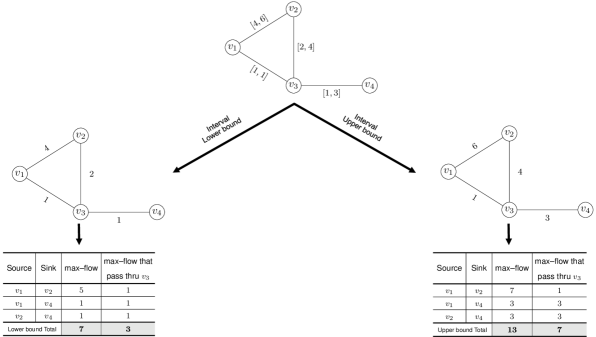
Figure 4: In the center is the interval-weighted network, on the left and right side are shown the weighted networks and the tables with the max-flow values for vertex $v_{3}$, when $v_{3}$ is neither a source nor a sink for the intervals lower and upper bounds, respectively.

Next, applications to two real-world interval-weighted networks further illustrates the proposed approaches.

5 Applications

In recent years, centrality measures have often been used in complex networks representing territorial units as tools to identify the central units (De Montis et al., 2007; De Montis et al., 2011; Cheng et al., 2015). We present the application of our centrality measures approach to two real-world interval-weighted networks. The first network represents the movements of daily commuters in mainland Portugal (by all means of transportation) between the 23 NUTS 3 Regions (henceforth, the “Interval-Weighted Commuters Network (IWCN)”) (source: INE – Statistics Portugal, Census 2011). The second application focuses on annual Merchandise trade (detailed products, exports in thousands of US dollars) between 28 European countries from 2003 to 2015 (henceforth, the “Interval-Weighted Trade Network (IWTN)”), analysing the commercial communities that emanate between these countries for the thirteen year period considered (henceforth, the “Interval–Weighted Trade Network (IWTN)”) (UNCTAD, 2016).

5.1 Network of Portuguese commuters

According to various authors, the flows of daily commuters can be conceived as a network (De Montis et al., 2007; Patuelli et al., 2007; De Montis et al., 2011, 2013; De Leo et al., 2013; Cheng et al., 2015; Xu et al., 2016; Barbosa et al., 2018; Zeng et al., 2018; Spadon et al., 2019). Hence, each vertex of the Interval-Weighted Commuters Network (IWCN) corresponds to a given NUTS 3 (which in turn represents the aggregation of commuter flows between the municipalities that constitute it) and the edges represent intervals ranging between the minimum flow larger than 50 commuters and the maximum flow of commuters between the corresponding NUTS 3. As represented in Figure 5a, the interval of commuters flow from NUTS $i\to j$ may be different from the one of $j\to i$. Therefore, the elements $o^{I}_{ij}$ of the symmetric interval-weighted adjacency matrix, $O^{I}$, denote the maximum variability of the bi-directional flows $ij$ and $ji$ between the NUTS $i$ and $j$ (Figure5b): $o^{I}_{ij}=\big{[}\min\{\underline{o}^{\prime}_{ij},\underline{o}^{\prime\prime}_{ji}\},\max\{\overline{o}^{\prime}_{ij},\overline{o}^{\prime\prime}_{ji}\}\big{]}=\big{[}\underline{o}_{ij},\overline{o}_{ij}\big{]}$. The option for this representation of flows is related to the fact that we do not want to study the orientation of these daily commuter fluxes, but just quantify the reciprocal attractiveness of the NUTS 3 pairs (De Montis et al., 2013). This kind of aggregation when the data are recorded at the same point in time and the statistical units to be analysed are not those for which the data was originally recorded, but constitute specific groups of those (level higher than the one at which the data was originally collected), is called contemporary aggregation (Brito, 2014).

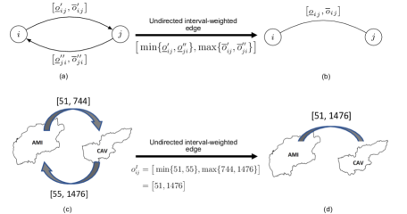
Figure 5: Conversion of directed interval-weighted edges into an undirected interval-weighted edge. (a) Bidirectional interval flows $i\to j$ and $j\to i$ between NUTS 3 $i$ and $j$, (b) Undirected interval flow between NUTS 3 $i$ and $j$, (c) and (d) are an example extracted from the real data.

The adjacency matrix elements are null, $o^{I}_{ij}=[0,0]$, when there is no commuter flow greater than 50 daily movements between NUTS 3 $i$ and $j$. By definition, we assume that there are no commuter flows within each NUTS 3, i.e., the network has no loops at initial vertices, which implies that the diagonal of the interval-weighted adjacency matrix consists of degenerate intervals with the value zero, $o^{I}_{ii}=[0,0]$.

Figure 6 shows the geographical distribution of NUTS 3 in mainland Portugal (Figure 6(a)), and the corresponding network of commuting movements between these NUTS 3, weighted by intervals denoting the maximum variability (Figure6(b)). This network has 23 vertices and 80 edges and is therefore considered a small network with low density (considering the intervals midpoints: $\text{graph density}=0.316$, $\text{diameter}=3$, $\text{average degree}=6.96$). For ease of reading, hereinafter we will only refer to Portugal instead of “mainland Portugal”.

(a)

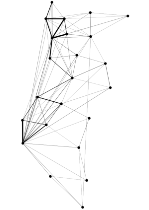
(b)

Figure 6: (a) Geographic representation of Portuguese NUTS 3, and (b) Topologic representation of the Portuguese NUTS 3 interval-weighted commuters network (IWCN).

5.1.1 Results – interval-weighted commuters network (IWCN)

In this section, applying the new centrality measures that incorporate the tuning parameter $\alpha$ of Opsahl’s et.al. (2010) for degree and the flow capacities of Freeman et.al. (1991) for betweenness and closeness, we aim at identifying which are the critical (most central) vertices in the interval-weighted network described above, i.e., which are the most central NUTS 3 in the country.

Interval-Weighted Degree Centrality (IWD)

Table 4 ranks in descending order the 23 NUTS 3 according to the degree centrality interval score for different values of the tuning parameter $\alpha$. Highlighted in gray are the cases where there was a shift in the interval rank classification with the change of the $\alpha$ value. To simplify our analysis, we will focus only on the two main regions, AML (Lisbon Metropolitan Area) and AMP (Porto Metropolitan Area). As expected, AML and AMP are the most central NUTS 3, irrespective of $\alpha$. A closer look however reveals that when the degree outcome is solely based on the number of edges, $\alpha=0$ (the edge weights are ignored and the degree is the same as if the network were binary), AML is the most central NUTS 3 and AMP comes in second place. The same occurs when we consider a tuning parameter such that $0<\alpha<1$ $(\alpha=0.5)$ (the degree would positively value both the number of edges and the edge weights), with weights varying approximately in $[159,436]$.
However, when the degree is based only on edge weights $(\alpha=1)$, AMP becomes the most central NUTS 3 with the degree varying in $[939,12997]$. Thus, we may conclude that AML is connected with more NUTS 3, but AMP despite having fewer connections, tends to have connections that involve more commuters. The same outcome is obtained if the tuning parameter is above one $(\alpha=1.5)$, which positively values edge strength and negatively values the number of edges $[7980,410954]$.

For the remaining NUTS 3 marked in gray there are also shifts in the degree interval rank classification with the change of the $\alpha$ parameter, which means that this measure, in fact, considers both the number of edges and the edges strength as well as being sensitive to the average edge weight of a vertex. In particular, Oeste (OES) clearly climbs in the ranking for $\alpha\geqslant 1$, showing that although not connected to many regions, its connections involve a large number of commuters; the opposite is observed for the Douro region (DOU).

Table 4: Degree centrality for the Interval-Weighted Commuters network (NUTS 3 ranked in descending order of interval rank for $\alpha=1$).

	Tuning parameter $(\alpha)$
	$\alpha=0$		$\alpha=0.5$		$\alpha=1$		$\alpha=1.5$
NUTS 3a	Degree interval	Interval rank	Degree interval	Interval rank	Degree interval	Interval rank	Degree interval	Interval rank
gray!25AMP	$[13,13]$	$2$	$[110.49,411.05]$	$2$	$[939,12997]$	$1$	$[7980.44,410953.80]$	$1$
gray!25AML	$[20,20]$	$1$	$[159.19,436.30]$	$1$	$[1267,9518]$	$2$	$[10084.40,207636.43]$	$2$
AVE	$[9,9]$	$5$	$[69.46,253.83]$	$3$	$[536,7159]$	$3$	$[4136.43,201909.75]$	$3$
CAV	$[9,9]$	$5$	$[69.91,249.27]$	$4$	$[543,6904]$	$4$	$[4217.73,191218.51]$	$4$
gray!25OES	$[6,6]$	$11$	$[46.15,178.43]$	$8$	$[355,5306]$	$5$	$[2730.66,157788.46]$	$5$
TES	$[7,7]$	$7$	$[51.91,189.04]$	$6$	$[385,5105]$	$6$	$[2855.24,137862.01]$	$6$
RLE	$[7,7]$	$7$	$[51.98,176.85]$	$7$	$[386,4468]$	$7$	$[2866.37,112880.97]$	$7$
gray!25RCO	$[12,12]$	$3$	$[92.04,210.09]$	$5$	$[706,3678]$	$8$	$[5415.22,64391.27]$	$11$
RAV	$[7,7]$	$7$	$[52.18,162.49]$	$9$	$[389,3772]$	$9$	$[2899.85,87560.56]$	$9$
MTJ	$[7,7]$	$7$	$[54.03,154.11]$	$10$	$[417,3393]$	$10$	$[3218.51,74701.06]$	$10$
gray!25LTJ	$[5,5]$	$13$	$[36.54,132.00]$	$12$	$[267,3485]$	$11$	$[1951.11,92006.64]$	$8$
gray!25AMI	$[5,5]$	$13$	$[37.22,115.20]$	$13$	$[277,2654]$	$12$	$[2061.74,61145.76]$	$12$
gray!25DOU	$[10,10]$	$4$	$[76.22,124.74]$	$11$	$[581,1556]$	$13$	$[4428.58,19409.50]$	$13$
VDL	$[6,6]$	$11$	$[52.31,87.02]$	$14$	$[456,1262]$	$14$	$[3975.32,18302.63]$	$14$
BSE	$[5,5]$	$13$	$[36.26,79.56]$	$15$	$[263,1266]$	$15$	$[1907.43,20144.92]$	$15$
gray!25BBA	$[4,4]$	$19$	$[36.72,59.06]$	$18$	$[337,872]$	$16$	$[3093.25,12874.93]$	$16$
gray!25ATA	$[5,5]$	$13$	$[44.05,58.40]$	$16$	$[388,682]$	$17$	$[3417.93,7965.11]$	$18$
gray!25ACE	$[5,5]$	$13$	$[37.42,62.13]$	$17$	$[280,772]$	$18$	$[2095.33,9592.70]$	$17$
TTM	$[5,5]$	$13$	$[39.69,46.85]$	$19$	$[315,439]$	$19$	$[2500.23,4113.50]$	$21$
ALG	$[4,4]$	$19$	$[31.81,43.27]$	$20$	$[253,468]$	$20$	$[2012.11,5062.19]$	$20$
AAL	$[3,3]$	$21$	$[23.75,39.72]$	$21$	$[188,526]$	$21$	$[1488.25,6964.95]$	$19$
ALI	$[3,3]$	$21$	$[23.17,34.07]$	$22$	$[179,387]$	$22$	$[1382.67,4395.48]$	$22$
BAL	$[3,3]$	$21$	$[24.80,29.55]$	$23$	$[205,291]$	$23$	$[1694.61,2866.02]$	$23$

• NUTS 3: ACE-Alentejo Central, ALI-Alentejo Litoral, ALG-Algarve, AAL-Alto Alentejo, AMI-Alto Minho, ATA-Alto Tâmega, AML-Área Metropolitana de Lisboa, AMP-Área Metropolitana do Porto, AVE-Ave, BAL-Baixo Alentejo, BBA-Beira Baixa, BSE-Beiras e Serra da Estrela, CAV-Cávado, DOU-Douro, LTJ-Lezíria do Tejo, MTJ-Médio Tejo, OES-Oeste, RAV-Região de Aveiro, RCO-Região de Coimbra, RLE-Região de Leiria, TES-Tâmega e Sousa, TTM-Terras de Trás-os-Montes, VDL-Viseu Dão Lafões.

Interval-Weighted Flow Centrality measures: Betweenness (IWFB) and Closeness (IWFC)

In Table 5 are shown the flow centrality measures for the 23 NUTS 3, ranked in descending order according to the flow betweenness centrality interval score. Regarding the Interval-Weighted Flow Betweenness (IWFB), the five most central NUTS 3 with the highest max-flow between all pairs of NUTS 3, that depends on them are: AML (Lisbon Metropolitan Area) $[15609,101172]$, followed by AMP (Porto Metropolitan Area) $[7348,95972]$, RCO (Coimbra Region) $[5306,55549]$, RAV (Aveiro Region) $[2329,39281]$ and RLE (Leiria Region) $[2805,35233]$. These are the areas of the most important cities (Lisbon and Porto), and then 3 regions in the center of the country, through which important commuter flows must pass.

Nevertheless, regarding the Interval-Weighted Flow Closeness (IWFC) centrality measure, the five most central NUTS 3 with the highest max-flow between them and the remaining NUTS 3 in the IWFC ranking (Table 5) are: AMP (Porto Metropolitan Area) $[8645,55083]$ ranks 1^st, AVE (Ave Region) $[8020,55083]$, CAV (Cávado Region) $[8048,54530]$, TES (Tâmega e Sousa Region) $[7154,51528]$ and AML (Lisbon Metropolitan Area) $[8645,49521]$. We find again the areas of Lisbon and Porto, as expected, plus three areas in the North of the country, known for being densely populated, therefore responsible for a greater flow of commuters between these regions.

It is noteworthy that AMP (Porto Metropolitan Area) becomes the most central region in the IWFC while in the IWFB it ranks 2^nd, AVE region ranks 2^nd in the IWFC while in the IWFB it ranks 10^th, CAV region ranks 3^nd in the IWFC while in the IWFB it ranks 6^th, TES region ranks 4^th in the IWFC while in the IWFB it ranks 14^th, whereas AML becomes 5^th in the IWFC while in the IWFB it ranks 1^st.

These differences between the IWFB and the IWFC centrality measures rankings are to be expected because the former measures the regions intermediary ability to communicate with other regions, high for AMP and AML, RCO, RAV, RLE, and the latter identifies the “communication power” of one region and the rest of the interval-weighted network, which is high for AMP, AML, AVE, CAV and TES.

Table 5: Flow centrality measures for the Interval-Weighted Commuters network (NUTS 3 ranked in descending order of interval rank for IWFB).

	max-flow (all pairs)b		Flow Betweenness		Flow Closeness
NUTS 3a	max-flow	max-flow rank	IWFBc	IWFB rank	IWFCd	IWFC rank
AML	$[68404,323339]$	$19$	$[15609,101172]$	$1$	$[8645,49521]$	$5$
AMP	$[68404,317777]$	$23$	$[7348,95972]$	$2$	$[8645,55083]$	$1$
RCO	$[68637,325757]$	$16$	$[5306,55549]$	$3$	$[8412,47103]$	$8$
RAV	$[69859,325331]$	$15$	$[2329,39281]$	$4$	$[7190,47529]$	$9$
RLE	$[69885,324177]$	$17$	$[2805,35233]$	$5$	$[7164,48683]$	$7$
CAV	$[69001,318330]$	$21$	$[3481,27263]$	$6$	$[8048,54530]$	$3$
MTJ	$[69663,327879]$	$14$	$[4345,23542]$	$7$	$[7386,44981]$	$10$
DOU	$[68887,347347]$	$11$	$[4711,22248]$	$8$	$[8162,25513]$	$13$
VDL	$[69429,350875]$	$10$	$[1932,19480]$	$9$	$[7620,21985]$	$14$
AVE	$[69029,317777]$	$22$	$[3671,14260]$	$10$	$[8020,55083]$	$2$
BSE	$[71490,352435]$	$9$	$[1357,15864]$	$11$	$[5559,20425]$	$15$
ACE	$[71217,357715]$	$7$	$[4286,9969]$	$12$	$[5832,15145]$	$17$
OES	$[70225,323339]$	$18$	$[2207,10424]$	$13$	$[6824,49521]$	$6$
TES	$[69895,321332]$	$20$	$[1783,9860]$	$14$	$[7154,51528]$	$4$
LTJ	$[71422,327051]$	$13$	$[2656,8175]$	$15$	$[5627,45809]$	$11$
BBA	$[70441,356215]$	$8$	$[1582,8196]$	$16$	$[6608,16645]$	$16$
ALG	$[71670,362851]$	$4$	$[2822,6668]$	$17$	$[5379,10009]$	$20$
ATA	$[69867,359155]$	$6$	$[1886,6097]$	$18$	$[7182,13705]$	$18$
AAL	$[72922,361807]$	$3$	$[1607,6235]$	$19$	$[4127,11053]$	$21$
AMI	$[71262,335269]$	$12$	$[1190,5380]$	$20$	$[5787,37591]$	$12$
ALI	$[73111,364442]$	$2$	$[2419,3782]$	$21$	$[3938,8418]$	$22$
TTM	$[70727,363402]$	$5$	$[2045,3950]$	$22$	$[6322,9458]$	$19$
BAL	$[72582,366458]$	$1$	$[2256,3542]$	$23$	$[4467,6402]$	$23$

• NUTS 3: ACE-Alentejo Central, ALI-Alentejo Litoral, ALG-Algarve, AAL-Alto Alentejo, AMI-Alto Minho, ATA-Alto Tâmega, AML-Área Metropolitana de Lisboa, AMP-Área Metropolitana do Porto, AVE-Ave, BAL-Baixo Alentejo, BBA-Beira Baixa, BSE-Beiras e Serra da Estrela, CAV-Cávado, DOU-Douro, LTJ-Lezíria do Tejo, MTJ-Médio Tejo, OES-Oeste, RAV-Região de Aveiro, RCO-Região de Coimbra, RLE-Região de Leiria, TES-Tâmega e Sousa, TTM-Terras de Trás-os-Montes, VDL-Viseu Dão Lafões.

• max-flow between all pairs of vertices, where the vertex $v_{i}$ is neither a source or a sink; ^c Interval–Weighted Flow Betweenness centrality; ^d Interval–Weighted Flow Betweenness centrality.

5.2 Network of Trade transactions between 28 European countries

The construction of the ‘Interval-Weighted Trade Network (IWTN)” of annual merchandise trade was done by aggregating the observations from the data corresponding to the values from $i\to j$ and from $j\to i$, between the 28 selected countries from 2003 to 2015 (UNCTAD, 2016), a temporal aggregation (Brito, 2014). Therefore, each vertex of the IWTN corresponds to one of the 28 European countries and the edges represent intervals varying between the minimum and maximum exports (in thousands of US dollars) among those countries.

Figure 7 shows the geographical distribution of the European countries belonging to the “Trade network” (Figure7a, and the corresponding network (Figure7b). This is a complete network (all vertices are connected between each other) which has 28 vertices and 378 edges and is therefore considered a small network in size but with high density ($\text{graph density}=1.0$, $\text{diameter}=1$, $\text{average degree}=27$).

(a)

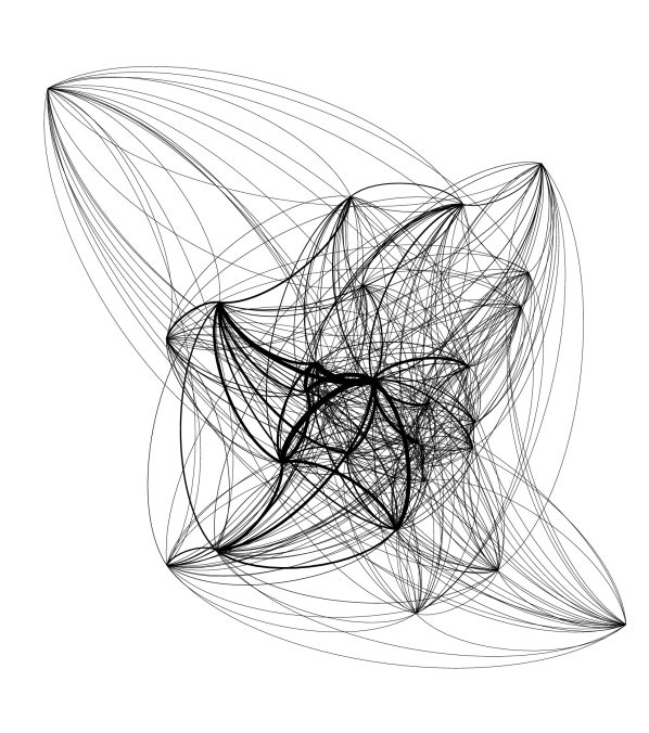
(b)

Figure 7: (a) Geographic representation of the European countries belonging to the “Trade network”, and (b) Topologic representation of the weighted “Trade network” (weighted by the intervals midpoint).

5.2.1 Results – interval-weighted trade network (IWTN)

Interval-Weighted Degree Centrality (IWD)

Table 6 below shows the degree centrality interval score for different values of the tuning parameter $\alpha$, ranking in descending order the 28 countries according to the degree centrality accounting only for the weight of the edges $\alpha=1$. Since this is a complete network, the number of edges attached to each one of the 28 countries analysed is the same (27 in this case), causing that shifting the tuning parameter $\alpha$ for the benchmark values $0.5,1$, and $1.5$, does not cause significant changes in degree rankings. As it might be expected, the major European economies appear as the most central ones: DE (Germany), FR (France), UK (United Kingdom), NL (Netherlands), BE (Belgium), IT (Italy) and ES (Spain).

Table 6: Degree centrality for the Interval-Weighted Trade network (Countries ranked in descending order of interval rank for $\alpha=1$).

	Tuning parameter $(\alpha)$
	$\alpha=0$		$\alpha=0.5$		$\alpha=1$		$\alpha=1.5$
Countriesa	Degree interval	Interval rank	Degree interval	Interval rank	Degree interval	Interval rank	Degree interval	Interval rank
DE	$[27,27]$	$1$	$[102326.85,175664.12]$	$1$	$[387806824.1,1142884585]$	$1$	$[1.469743e+12,7.435697e+12]$	$1$
FR	$[27,27]$	$1$	$[78465.04,124536.28]$	$2$	$[228028235.1,574417976]$	$2$	$[6.626757e+11,2.649477e+12]$	$2$
UK	$[27,27]$	$1$	$[68417.45,121986.45]$	$3$	$[173368436.3,551136848]$	$3$	$[4.393121e+11,2.490046e+12]$	$3$
NL	$[27,27]$	$1$	$[64452.68,122444.18]$	$4$	$[153857308.5,555280599]$	$4$	$[3.672783e+11,2.518181e+12]$	$4$
BE	$[27,27]$	$1$	$[62336.59,109086.05]$	$5$	$[143920368.4,440732048]$	$5$	$[3.322779e+11,1.780656e+12]$	$5$
IT	$[27,27]$	$1$	$[65458.24,105143.01]$	$6$	$[158695591.1,409446369]$	$6$	$[3.847383e+11,1.594460e+12]$	$6$
ES	$[27,27]$	$1$	$[53541.28,89445.76]$	$7$	$[106172922.1,296316422]$	$7$	$[2.105420e+11,9.816388e+11]$	$7$
CH	$[27,27]$	$1$	$[40808.66,82191.47]$	$8$	$[61679515.7,250201410]$	$8$	$[9.322439e+10,7.616453e+11]$	$8$
AT	$[27,27]$	$1$	$[40815.39,68822.90]$	$9$	$[61699855.2,175429336]$	$9$	$[9.327051e+10,4.471688e+11]$	$10$
PL	$[27,27]$	$1$	$[33190.64,71855.75]$	$10$	$[40800682.2,191231455]$	$10$	$[5.015558e+10,5.089289e+11]$	$9$
SE	$[27,27]$	$1$	$[39661.81,64544.17]$	$11$	$[58261436.6,154294441]$	$11$	$[8.558347e+10,3.688447e+11]$	$11$
gray!25NO	$[27,27]$	$1$	$[25755.63,67581.50]$	$13$	$[24568609.2,169157757]$	$12$	$[2.343630e+10,4.234050e+11]$	$12$
gray!25CZ	$[27,27]$	$1$	$[32407.79,64297.41]$	$12$	$[38898697.0,153116925]$	$13$	$[4.668966e+10,3.646304e+11]$	$13$
gray!25IE	$[27,27]$	$1$	$[29851.83,53765.41]$	$15$	$[33004874.4,107063662]$	$14$	$[3.649096e+10,2.131971e+11]$	$14$
gray!25DK	$[27,27]$	$1$	$[32359.85,52121.61]$	$14$	$[38783706.3,100617119]$	$15$	$[4.648278e+10,1.942343e+11]$	$15$
HU	$[27,27]$	$1$	$[29042.88,49959.48]$	$16$	$[31240334.1,92442580]$	$16$	$[3.360405e+10,1.710512e+11]$	$16$
gray!25SK	$[27,27]$	$1$	$[20855.16,46253.34]$	$19$	$[16108809.1,79235966]$	$17$	$[1.244266e+10,1.357381e+11]$	$17$
PT	$[27,27]$	$1$	$[25589.03,43750.86]$	$18$	$[24251801.6,70893996]$	$18$	$[2.298445e+10,1.148768e+11]$	$18$
gray!25FI	$[27,27]$	$1$	$[26188.34,43348.28]$	$17$	$[25401081.1,69595323]$	$19$	$[2.463749e+10,1.117347e+11]$	$19$
EL	$[27,27]$	$1$	$[13783.88,39116.17]$	$20$	$[7036862.9,56669429]$	$20$	$[3.592417e+09,8.209966e+10]$	$20$
LU	$[27,27]$	$1$	$[15505.02,30508.99]$	$21$	$[8903912.7,34474010]$	$21$	$[5.113161e+09,3.895434e+10]$	$21$
SI	$[27,27]$	$1$	$[15318.91,28393.76]$	$22$	$[8691444.8,29859460]$	$22$	$[4.931239e+09,3.140082e+10]$	$22$
gray!25LT	$[27,27]$	$1$	$[9470.52,25318.00]$	$24$	$[3321876.1,23740782]$	$23$	$[1.165181e+09,2.226182e+10]$	$23$
gray!25HR	$[27,27]$	$1$	$[10479.74,24328.75]$	$23$	$[4067588.9,21921777]$	$24$	$[1.578788e+09,1.975294e+10]$	$24$
LV	$[27,27]$	$1$	$[6983.80,20195.38]$	$25$	$[1806423.4,15105675]$	$25$	$[4.672480e+08,1.129870e+10]$	$25$
CY	$[27,27]$	$1$	$[2968.57,17697.96]$	$26$	$[326386.2,11600664]$	$26$	$[3.588524e+07,7.604005e+09]$	$26$
IS	$[27,27]$	$1$	$[5444.54,14558.85]$	$27$	$[1097891.1,7850370]$	$27$	$[2.213895e+08,4.233049e+09]$	$28$
MT	$[27,27]$	$1$	$[3984.12,14765.58]$	$28$	$[587897.3,8074900]$	$28$	$[8.675016e+07,4.415947e+09]$	$27$

• Countries: AT-Austria, BE-Belgium, HR-Croatia, CY-Cyprus, CZ-Czech Republic, DK-Denmark, FI-Finland, FR, France, DE-Germany, EL-Greece, HU-Hungary, IS-Iceland, IE-Ireland, IT-Italy, LV-Latvia, LT, Lithuania, LU-Luxembourg, MT-Malta, NL-Netherlands, NO-Norway, PL-Poland, PT-Portugal, SK-Slovakia, SI-Slovenia, ES-Spain, SE-Sweden, CH-Switzerland, UK-United Kingdom.

Interval-Weighted Flow Centrality measures: Betweenness (IWFB) and Closeness (IWFC)

Table 7 shows the flow centrality measures for the 28 European countries analysed, ranked in descending order according to the flow betweenness centrality interval score. Regarding the Interval-Weighted Flow Betweenness (IWFB), DE (Germany) is the most central European country, i.e., the country through which most flows must pass, followed by UK (United Kingdom), FR (France). NL (Netherlands), IT (Italy), BE (Belgium) and ES (Spain).

Nevertheless, regarding the Interval-Weighted Flow Closeness (IWFC) centrality measure, FR (France) becomes the most central European country, i.e., the country that centralizes most annual merchandise trade in the considered years (Table 5).

It is noteworthy that SE (Sweden) ranks 11^th in the IWFC while in the IWFB it ranks 8^th, putting in evidence its intermediation role. On the contrary, CH (Switzerland) ranks 8^th in the IWFC whereas in the IWFB it ranks 10^th.

Table 7: Flow centrality measures for the Interval–Weighted Trade network (Countries ranked in descending order of interval rank for IWFB).

	max–flow (all pairs)b		Flow Betweenness		Flow Closeness
Countriesa	max–flow	max–flow rank	IWFBc	IWFB rank	IWFCd	IWFC rank
DE	$[7413003807,26769887480]$	$27$	$[2185413096,6566281708]$	$1$	$[1453915546,4649907299]$	$1$
UK	$[7468330607,26797312358]$	$26$	$[838121364,2978511281]$	$2$	$[1398588745,4622482420]$	$3$
FR	$[7413003807,26769887480]$	$27$	$[881547435,2328131952]$	$3$	$[1453915546,4649907299]$	$1$
NL	$[7510857142,26789024857]$	$25$	$[557453333,2159124156]$	$4$	$[1356062210,4630769922]$	$4$
IT	$[7496342294,27253669475]$	$23$	$[633270908,2072687573]$	$5$	$[1370577058,4166125304]$	$6$
BE	$[7550604902,27128526758]$	$24$	$[453239198,1752227012]$	$6$	$[1316314450,4291268020]$	$5$
ES	$[7739342134,27819319211]$	$22$	$[401228536,1484669303]$	$7$	$[1127577219,3600475569]$	$7$
SE	$[8033667545,28840293295]$	$18$	$[383023300,1051732575]$	$8$	$[833251808,2579501489]$	$11$
PL	$[8190814334,28508798969]$	$19$	$[157392715,1013176935]$	$9$	$[676105018,2910995812]$	$10$
CH	$[8006322912,28096009281]$	$21$	$[179713794,894364013]$	$10$	$[860596441,3323785497]$	$8$
AT	$[8006180535,28635215917]$	$20$	$[243111799,784248460]$	$11$	$[860738817,2784578860]$	$9$
CZ	$[8209834186,28853245967]$	$17$	$[163521022,799346141]$	$12$	$[657085166,2566548813]$	$12$
NO	$[8397620711,28691660132]$	$16$	$[143183388,799696175]$	$13$	$[469298641,2728134649]$	$13$
DK	$[8211099084,29489690179]$	$14$	$[206979675,633196218]$	$14$	$[655820269,1930104598]$	$15$
HU	$[8303384091,29604133730]$	$13$	$[119391634,522797634]$	$15$	$[563535262,1815661052]$	$16$
SK	$[8541120505,29802232940]$	$10$	$[87072347,546677594]$	$16$	$[325798847,1617561842]$	$19$
FI	$[8385133632,29957781899]$	$11$	$[134826401,453203323]$	$17$	$[481785719,1462012881]$	$18$
IE	$[8280445067,29405885128]$	$15$	$[98708914,465212077]$	$18$	$[586474286,2013909657]$	$14$
PT	$[8402689632,29935704453]$	$12$	$[92016005,328147696]$	$19$	$[464229719,1484090322]$	$17$
EL	$[8707937169,30190447994]$	$9$	$[27673872,296713444]$	$20$	$[158982184,1229346789]$	$20$
SI	$[8674845530,30704451956]$	$7$	$[43474161,211867658]$	$21$	$[192073822,715342828]$	$22$
LT	$[8786697603,30832944183]$	$6$	$[21970780,204033734]$	$22$	$[80221748,586850590]$	$23$
HR	$[8770291922,30872962304]$	$5$	$[24009255,184513589]$	$23$	$[96627429,546832480]$	$24$
LV	$[8821553016,31029732634]$	$4$	$[14592275,160007089]$	$24$	$[45366336,390062134]$	$25$
LU	$[8670808641,30612160946]$	$8$	$[23517667,135821723]$	$25$	$[196110712,807633828]$	$21$
CY	$[8858106924,31113852903]$	$3$	$[2678597,98121070]$	$26$	$[8812427,305941870]$	$26$
IS	$[8838557792,31207834800]$	$2$	$[5273107,54270679]$	$27$	$[28361561,211959990]$	$27$
MT	$[8851307637,31201997000]$	$1$	$[1342859,50523695]$	$28$	$[15611716,217797770]$	$28$

• Countries: AT-Austria, BE-Belgium, HR-Croatia, CY-Cyprus, CZ-Czech Republic, DK-Denmark, FI-Finland, FR, France, DE-Germany, EL-Greece, HU-Hungary, IS-Iceland, IE-Ireland, IT-Italy, LV-Latvia, LT, Lithuania, LU-Luxembourg, MT-Malta, NL-Netherlands, NO-Norway, PL-Poland, PT-Portugal, SK-Slovakia, SI-Slovenia, ES-Spain, SE-Sweden, CH-Switzerland, UK-United Kingdom.

• max–flow between between all pairs of vertices, where the vertex $v_{i}$ is neither a source or a sink; ^c Interval–Weighted Flow Betweenness centrality; ^d Interval–Weighted Flow Closeness centrality.

6 Concluding remarks

In recent years, the term “Big Data” emerged, and new approaches arise to deal with large amounts of information, including the possibility to aggregate data to provide more manageably-sized datasets. These new approaches may consist of considering aggregated (e.g. interval) data, keeping the information on the intrinsic variability in order to capture the original dispersion of the data. However, the definitions of basic statistical notions do not apply automatically in this aggregated data, and well-established properties are no longer straightforward. Furthermore, when we use such aggregated data on complex structures, such as network data, the situation may become harder do handle. Therefore, to apply statistical and multivariate data analysis techniques to interval data in network structures requires proper consideration and often the design of new approaches and appropriate techniques. In this paper we provide a novel contribution to network science in that we use aggregate interval data to describe the weights of networks’ edges, giving rise to the concept of Interval-Weighted Networks (IWN). We start by generalizing the three classical centrality measures, degree, closeness and betweenness, for the general case of IWN, with a triple motivation: firstly, we try to establish a benchmark for these measures when using intervals defined by the minimum and maximum observed weights on the edges of the IWN; secondly, extend the degree centrality based on Opsahl et al. (2010) concept of a tuning parameter to give relevance either to tie weights or number of ties alternatively; and thirdly, generalize closeness and betweenness based on network flows, where with each edge is assigned a flow which maximizes the total flow between a pair of vertices and using Ford and Fulkerson’s max-flow method (Ford and Fulkerson, 1956; Freeman et al., 1991).

The experiments carried out on an artificial network and on two real-world networks (IWCN and IWTN) have shown that, for the Interval-Weighted Degree (IWD), as expected, the variation of the tuning parameter $\alpha$ to give relevance either to tie weights or number of ties alternatively (Opsahl et al., 2010) affects the ranking centrality of the vertices. In the IWCN it changes the topological importance of some NUTS 3 as an attraction point (center). In the IWTN, as the number of connections is the same for all vertices (the 28 European countries), i.e., is a complete network, the change is residual.

Similarly, it has been found that the use of intervals has made it possible to capture a variation in the flow betweenness (IWFB) and flow closeness (IWFC), in terms of all paths connecting pairs of vertices, and not based only on geodesic paths.

The joint use of the two measures allowed putting in evidence the regions/countries that play an important intermediation role, distinguishing them from the regions/countries that register a high flow with the rest of the network.

Acknowledgements:

This work was financed by the Portuguese funding agency,FCT - Fundação para a Ciência e a Tecnologia, within project UIDB/50014/2020. This research has also received funding from the European Union’s Horizon 2020 research and innovation program ”FIN-TECH: A Financial supervision and Technology compliance training programme” under the grant agreement No 825215 (Topic: ICT-35-2018, Type of action: CSA).

Appendix A: Lexicographic Order

Given an interval-weighted network (a triplet, see Figure 8(a)), consider that each of the edge intervals is described by the lower (L) and upper limit (U) and the respective quartiles $(Q_{1},Q_{2},Q_{3})$ (assuming a uniform distribution), as shown in Figure 8(b), and in the table of the Figure 8c (table).

(a)

(b)

	Intervals
	$w_{12}=[2,8]$	$w_{13}=[1,5]$	$w_{23}=[0,10]$
gray!20L	$2$	$1$	$0$
$Q_{1}$	$3.5$	$2$	$2.5$
$Q_{2}$	$5$	$3$	$5$
$Q_{3}$	$6.5$	$4$	$7.5$
gray!20U	$8$	$5$	$10$

• L, U – interval lower and upper bounds.

• $Q_{1},Q_{2},Q_{3}$ – 1^st, 2^nd and 3^rd quartiles.

(c)

Figure 8: Example of the values used for each interval of the IWN.

Table 8 below shows the outcome of the max-flow calculations for each of the $5^{3}=125$ possible combinations, following the lexicographic order, for these three intervals. We observe that the value of the “Max Flow” always increases when the value considered for at least one of the values increases. Therefore, at each edge, the minimum and maximum flows are obtained with the corresponding minimum and maximum values.

Table 8: Lexicographic order of three intervals each with five values.

$w_{12},w_{13}$ and $w_{23}$ – are interval–weighted values of the edges in a connected interval–weighted network with three vertices (triplet).
Max Flow – is the Ford & Fulkerson’s maximum flow for each of the 125 weighted networks generated in the lexicographic order.

References

- Ahuja et al. (1993) Ahuja, R. K., T. L. Magnanti, and J. B. Orlin (1993). Network Flows. Theory, algorithms, and applications. New Jersey: Prentice Hall.
- Barabasi (2016) Barabasi, A.-L. (2016). Network Science. Cambridge University Press.
- Barbosa et al. (2018) Barbosa, H., M. Barthelemy, G. Ghoshal, C. R. James, M. Lenormand, T. Louail, R. Menezes, J. J. Ramasco, F. Simini, and M. Tomasini (2018). Human mobility: Models and applications. Physics Reports 734, 1–74.
- Barigozzi et al. (2011) Barigozzi, M., G. Fagiolo, and G. Mangioni (2011). Identifying the community structure of the international-trade multi-network. Physica A: Statistical Mechanics and its Applications 390(11), 2051–2066.
- Barrat et al. (2004) Barrat, A., M. Barthelemy, R. Pastor-Satorras, and A. Vespignani (2004). The architecture of complex weighted networks. PNAS 101(11), 3747–3752.
- Billard and Diday (2007) Billard, L. and E. Diday (2007). Symbolic Data Analysis: Conceptual Statistics and Data Mining. Wiley Series in Computational Statistics. West Sussex, England: Wiley.
- Bonacich (1972) Bonacich, P. (1972). Factoring and weighting approaches to status scores and clique identification. The Journal of Mathematical Sociology 2(1), 113–120.
- Bonacich (1987) Bonacich, P. (1987). Power and centrality: A family of measures. American journal of sociology 92, 1170–1182.
- Borgatti (2005) Borgatti, S. P. (2005). Centrality and network flow. Social Networks 27(1), 55–71.
- Borgatti and Everett (2006) Borgatti, S. P. and M. G. Everett (2006). A Graph-theoretic perspective on centrality. Social Networks 28(4), 466–484.
- Bozhenyuk et al. (2017) Bozhenyuk, A. V., E. M. Gerasimenko, J. Kacprzyk, and I. N. Rozenberg (2017). Flows in Networks Under Fuzzy Conditions, Volume 346. Studies in Fuzziness and Soft Computing.
- Brandes (2001) Brandes, U. (2001). A Faster Algorithm for Betweenness Centrality. Journal of mathematical sociology 25(2), 163–177.
- Brandes (2008) Brandes, U. (2008). On variants of shortest-path betweenness centrality and their generic computation. Social Networks 30(2), 136–145.
- Brandes et al. (2016) Brandes, U., S. P. Borgatti, and L. C. Freeman (2016). Maintaining the duality of closeness and betweenness centrality. Social Networks 44, 153–159.
- Brandes and Fleischer (2005) Brandes, U. and D. Fleischer (2005). Centrality measures based on current flow. In Stacs 2005, Proceedings, pp. 533–544.
- Brin and Page (1998) Brin, S. and L. Page (1998). The anatomy of a large-scale hypertextual Web search engine. Computer Networks and Isdn Systems 30(1-7), 107–117.
- Brito (2014) Brito, P. (2014). Symbolic Data Analysis: another look at the interaction of Data Mining and Statistics. Wiley Interdisciplinary Reviews: Data Mining and Knowledge Discovery 4(4), 281–295.
- Cheng et al. (2015) Cheng, Y.-Y., R. K.-W. Lee, E.-P. Lim, and F. Zhu (2015). Measuring Centralities for Transportation Networks Beyond Structures. In P. Kazienko and N. V. Chawla (Eds.), Applications of Social Media and Social Network Analysis, Lecture Notes in Social Networks, pp. 23–39. Cham: Springer International Publishing.
- Couso and Dubois (2014) Couso, I. and D. Dubois (2014). Statistical reasoning with set-valued information: Ontic vs. epistemic views. International Journal of Approximate Reasoning 55(7), 1502–1518.
- Dawood (2011) Dawood, H. (2011). Theories of Interval Arithmetic. Mathematical Foundations and Applications. LAP Lambert Academic Publishing.
- De Leo et al. (2013) De Leo, V., G. Santoboni, F. Cerina, M. Mureddu, L. Secchi, and A. Chessa (2013). Community core detection in transportation networks. Physical Review E 88(4), 3.
- De Montis et al. (2007) De Montis, A., M. Barthelemy, A. Chessa, and A. Vespignani (2007). The Structure of Interurban Traffic: A Weighted Network Analysis. Environment and Planning B: Planning and Design 34(5), 905–924.
- De Montis et al. (2011) De Montis, A., S. Caschili, and A. Chessa (2011). Time evolution of complex networks: commuting systems in insular Italy. Journal of Geographical Systems 13(1), 49–65.
- De Montis et al. (2013) De Montis, A., S. Caschili, and A. Chessa (2013). Commuter networks and community detection: A method for planning sub regional areas. The European Physical Journal Special Topics 215(1), 75–91.
- Dijkstra (1959) Dijkstra, E. W. (1959). A note on two problems in connection with graphs. Numer Math 1, 269–271.
- Du et al. (2014) Du, Y., C. Gao, Y. Hu, S. Mahadevan, and Y. Deng (2014). A new method of identifying influential nodes in complex networks based on TOPSIS. Physica A: Statistical Mechanics and its Applications 399, 57–69.
- Eurostat (2016) Eurostat (2016). Commission Regulation (EU) 2016/2066 of 21 November 2016 amending the annexes to Regulation (EC) No 1059/2003 of the European Parliament and of the Council on the establishment of a common classification of territorial units for statistics (NUTS). Available online at: https://ec.europa.eu/eurostat/web/nuts/background (accessed: 15.06.2017).
- Ford and Fulkerson (1956) Ford, L. R. and D. R. Fulkerson (1956). Maximal flow through a network. Canadian journal of Mathematics 8(3), 399–404.
- Ford and Fulkerson (1957) Ford, L. R. and D. R. Fulkerson (1957). A simple algorithm for finding maximal network flows and an application to the Hitchcock problem. Canada Journal of Mathematics 9, 210–218.
- Ford and Fulkerson (1962) Ford, L. R. and D. R. Fulkerson (1962). Flows in Networks. NJ: Princeton University Press.
- Freeman (1977) Freeman, L. C. (1977). A set of measures of centrality based on betweenness. Sociometry, 35–41.
- Freeman (1979) Freeman, L. C. (1979). Centrality in social networks conceptual clarification. Social Networks 1(3), 215–239.
- Freeman et al. (1991) Freeman, L. C., S. P. Borgatti, and D. R. White (1991). Centrality in valued graphs: A measure of betweenness based on network flow. Social Networks 13(2), 141–154.
- Garas et al. (2012) Garas, A., F. Schweitzer, and S. Havlin (2012). A k-shell decomposition method for weighted networks. New Journal of Physics 14(8), 083030.
- Ghalmane et al. (2019) Ghalmane, Z., M. El Hassouni, C. Cherifi, and H. Cherifi (2019). Centrality in modular networks. EPJ Data Sci. 8, 1–27.
- Gómez et al. (2013) Gómez, D., J. R. Figueira, and A. Eusébio (2013). Modeling centrality measures in social network analysis using bi-criteria network flow optimization problems. European Journal of Operational Research 226(2), 354–365.
- Gómez et al. (2003) Gómez, D., E. González-Arangüena, C. Manuel, G. Owen, M. del Pozo, and J. Tejada (2003). Centrality and power in social networks - a game theoretic approach. Mathematical Social Sciences 46, 27–54.
- Granovetter (1973) Granovetter, M. S. (1973). The strength of weak ties. American journal of sociology 78(6), 1360–1380.
- Grzegorzewski and Śpiewak (2017) Grzegorzewski, P. and M. Śpiewak (2017). The Sign Test for Interval-Valued Data. In Soft Methods for Data Science. SMPS 2016. Advances in Intelligent Systems and Computing, pp. 269–276. Cham: Springer International Publishing.
- Guerra and Stefanini (2012) Guerra, M. L. and L. Stefanini (2012). A comparison index for interval ordering based on generalized Hukuhara difference. Soft Computing 16(11), 1931–1943.
- Hossain (2009) Hossain, A. (2009). Most Reliable Route Method and Algorithm Based on Interval Possibilities for a Cyclic Network. Cybernetics and Information Technologies 9, 81–92.
- Hossain and Gatev (2010) Hossain, A. and G. Gatev (2010). Method and Algorithm for Interval Maximum Expected Flow in a Network. Information technologies and control 1, 18–24.
- Hu and Wang (2006) Hu, B. Q. and S. Wang (2006). A novel approach in uncertain programming part I: New arithmetic and order relation for interval numbers. Journal of Industrial and Management Optimization 2(4), 351–371.
- Hu and Hu (2008) Hu, C. and P. Hu (2008). Interval-Weighted Graphs and Flow Networks. In C. Hu, R. B. Kearfott, A. d. Korvin, and V. Kreinovich (Eds.), Knowledge Processing with Interval and Soft Computing, pp. 1–16. London: Springer London.
- Karmakar and Bhunia (2012) Karmakar, S. and A. K. Bhunia (2012). A Comparative Study of Different Order Relations of Intervals. Reliable Computing 16, 38–72.
- Karmakar and Bhunia (2014) Karmakar, S. and A. K. Bhunia (2014). Uncertain constrained optimization by interval-oriented algorithm. Journal of the Operational Research Society 65(1), 73–87.
- Katz (1953) Katz, L. (1953). A new status index derived from sociometric analysis. Psychometrika 18, 39–43.
- Lu et al. (2016) Lu, L., D. Chen, X.-L. Ren, Q.-M. Zhang, Y.-C. Zhang, and T. Zhou (2016). Vital nodes identification in complex networks. Physics Reports 650, 1–63.
- Lu et al. (2016) Lu, L., T. Zhou, Q.-M. Zhang, and H. E. Stanley (2016). The H-index of a network node and its relation to degree and coreness. Nature Communications 7, 1–7.
- Martin et al. (2014) Martin, T., X. Zhang, and M. Newman (2014). Localization and centrality in networks. Physical Review E 90(5), 052808.
- Moore et al. (2009) Moore, R. E., R. B. Kearfott, and M. J. Cloud (2009). Introduction to Interval Analysis. Philadelphia: SIAM.
- Newman (2005) Newman, M. (2005). A measure of betweenness centrality based on random walks. Social Networks 27(1), 39–54.
- Newman (2018) Newman, M. (2018). Networks (2 ed.). Oxford University Press.
- Newman (2001) Newman, M. E. J. (2001). Scientific collaboration networks. II. Shortest paths, weighted networks, and centrality. Physical Review E 64(1), 016132.
- Opsahl et al. (2010) Opsahl, T., F. Agneessens, and J. Skvoretz (2010). Node centrality in weighted networks: Generalizing degree and shortest paths. Social Networks 32(3), 245–251.
- Patuelli et al. (2007) Patuelli, R., A. Reggiani, S. P. Gorman, P. Nijkamp, and F.-J. Bade (2007). Network Analysis of Commuting Flows: A Comparative Static Approach to German Data. Networks and Spatial Economics 7(4), 315–331.
- Qiao et al. (2017) Qiao, T., W. Shan, and C. Zhou (2017). How to Identify the Most Powerful Node in Complex Networks? A Novel Entropy Centrality Approach. Entropy 19(11), 614.
- Rodrigues (2019) Rodrigues, F. A. (2019). Network Centrality: An Introduction. In A Mathematical Modeling Approach from Nonlinear Dynamics to Complex Systems, pp. 177–196. Cham: Springer International Publishing.
- Sabidussi (1966) Sabidussi, G. (1966). The centrality index of a graph. Psychometrika 31(4), 581–603.
- Schroeder et al. (2004) Schroeder, J., A. P. Guedes, and E. P. Duarte, Jr (2004). Computing the Minimum Cut and Maximum Flow of Undirected Graphs. Technical Report RT-DINF 003/2004.
- Sengupta and Pal (2009) Sengupta, A. and T. K. Pal (2009). Fuzzy Preference Ordering of Interval Numbers in Decision Problems. Springer Science & Business Media.
- Spadon et al. (2019) Spadon, G., A. C. P. L. F. de Carvalho, J. F. Rodrigues-Jr, and L. G. A. Alves (2019). Reconstructing commuters network using machine learningand urban indicators. Technical Report 11801.
- Stefanini et al. (2019) Stefanini, L., M. L. Guerra, and B. Amicizia (2019). Interval Analysis and Calculus for Interval-Valued Functions of a Single Variable. Part I: Partial Orders, gH-Derivative, Monotonicity. Axioms 8(4), 113.
- Stephenson and Zelen (1989) Stephenson, K. and M. Zelen (1989). Rethinking centrality: methods and examples. Social Networks 11(1), 1–37.
- Traag (2014) Traag, V. (2014). Algorithms and Dynamical Models for Communities and Reputation in Social Networks. Springer.
- UNCTAD (2016) UNCTAD (2016). Merchandise trade matrix – detailed products, exports in thousands of United States dollars, annual. Available online at: https://https://unctadstat.unctad.org/wds/ReportFolders/reportFolders.aspx?sCS_referer=&sCS_ChosenLang=en (accessed: 09.09.2016).
- Valente and Foreman (1998) Valente, T. W. and R. K. Foreman (1998). Integration and radiality: measuring the extent of an individual’s connectedness and reachability in a network. Social Networks 20, 89–105.
- Wu et al. (2019) Wu, M., S. He, Y. Zhang, J. Chen, Y. Sun, Y.-Y. Liu, J. Zhang, and H. V. Poor (2019). A tensor-based framework for studying eigenvector multicentrality in multilayer networks. Proceedings of the National Academy of Sciences 116(31), 15407–15413.
- Xu et al. (2016) Xu, Q., B. Mao, and Y. Bai (2016). Network structure of subway passenger flows. arXiv.org (3), 033404–.
- Zeng et al. (2018) Zeng, L., J. Liu, Y. Qin, L. Wang, and J. Yang (2018). A Passenger Flow Control Method for Subway Network Based on Network Controllability. Discrete Dynamics in Nature and Society 2018(6), 1–12.
- Zhang et al. (2020) Zhang, Y., C. Shao, S. He, and J. Gao (2020). Resilience centrality in complex networks. Physical Review E 101(2), 022304.