Exploring Counterfactual Explanations Through the Lens of Adversarial Examples: A Theoretical and Empirical Analysis

Abstract

As machine learning (ML) models become more widely deployed in high-stakes applications, counterfactual explanations have emerged as key tools for providing actionable model explanations in practice. Despite the growing popularity of counterfactual explanations, a deeper understanding of these explanations is still lacking. In this work, we systematically analyze counterfactual explanations through the lens of adversarial examples. We do so by formalizing the similarities between popular counterfactual explanation and adversarial example generation methods identifying conditions when they are equivalent. We then derive the upper bounds on the distances between the solutions output by counterfactual explanation and adversarial example generation methods, which we validate on several real world data sets. By establishing these theoretical and empirical similarities between counterfactual explanations and adversarial examples, our work raises fundamental questions about the design and development of existing counterfactual explanation algorithms.

1 Introduction

With the increasing use of Machine learning (ML) models in critical domains, such as health care and law enforcement, it becomes important to ensure that their decisions are robust and explainable. To this end, several approaches have been proposed in recent literature to explain the complex behavior of ML models [32, 29, 24, 33]. One such popular class of explanations designed to provide recourse to individuals adversely impacted by algorithmic decisions are counterfactual explanations [40, 36, 4, 38]. For example, in a credit scoring model where an individual loan application is denied, a counterfactual explanation can highlight the minimal set of changes the individual can make to obtain a positive outcome [27, 20]. Algorithms designed to output counterfactual explanations often attempt to find a closest counterfactual for which the model prediction is positive [40, 36, 27, 20].

Adversarial examples, on the other hand, were proposed to highlight how vulnerabilities of ML models can be exploited by (malicious) adversaries  [34, 3, 9]. These adversarial examples are usually also obtained by finding minimal perturbations to a given data instance such that the model prediction changes [14, 8, 26].

Conceptually, adversarial examples and counterfactual explanations solve a similar optimization problem [12, 40, 9]. Techniques generating adversarial examples and counterfactual explanations use distance or norm constraints in the objective function to enforce the notion of minimal perturbations. While adversarial methods generate instances that are semantically indistinguishable from the original instance, counterfactual explanations or algorithmic recourse, encourage minimal changes to an input so that so that a user can readily act upon these changes to obtain the desired outcome. In addition, some methods in both lines of work use manifold-based constraints to find natural adversarial examples [41] or realistic counterfactual explanations by restricting them to lie on the data manifold [17, 27].

While the rationale of producing a counterfactual close to the original instance is motivated by the desideratum that counterfactuals should be actionable and easily understandable, producing close instances on the other side of the decision boundary could just as easily indicate adversarial activity. This begs the question to what extent do counterfactual explanation algorithms return solutions that resemble adversarial examples. However, there has been little to no work on systematically analyzing the aforementioned connections between the literature on counterfactual explanations and adversarial examples.

Present Work. In this work, we approach the study of similarities between counterfactual explanations and adversarial examples from the perspective of counterfactual explanations for algorithmic recourse. Therefore, we consider consequential decision problems (e.g., loan applications) commonly employed in recourse literature and our choices of data modalities (i.e., tabular data) and algorithms are predominantly motivated by this literature. In particular, we make one of the first attempts at establishing theoretical and empirical connections between state-of-the-art counterfactual explanation and adversarial example generation methods.

More specifically, we analyze these similarities by bounding the distances between the solutions of salient counterfactual explanation and popular adversarial example methods for locally linear approximations. Our analysis demonstrates that several popular counterfactual explanation and adversarial example generation methods such as the ones proposed by Wachter et al. [40] and Carlini and Wagner [8], Moosavi-Dezfooli et al. [26], are equivalent for certain hyperparameter choices. Moreover, we demonstrate that C-CHVAE and the natural adversarial attack (NAE) [41] provide similar solutions for certain generative model choices.

Finally, we carry out extensive experimentation with multiple synthetic and real-world data sets from diverse domains such as financial lending and criminal justice to validate our theoretical findings. We further probe these methods empirically to validate the similarity between the counterfactuals and adversarial examples output by several state-of-the-art methods. Our results indicate that counterfactuals and adversarial examples output by manifold-based methods such as NAE and C-CHVAE are more similar compared to those generated by other techniques. By establishing these and other theoretical and empirical similarities, our work raises fundamental questions about the design and development of existing counterfactual explanation algorithms.

2 Related Work

This work lies at the intersection of counterfactual explanations and adversarial examples in machine learning. Below we discuss related work for each of these topics and their connection.

Adversarial examples. Adversarial examples are obtained by making infinitesimal perturbations to input instances such that they force a ML model to generate adversary-selected outputs. Algorithms designed to successfully generate these examples are called Adversarial attacks [34, 14]. Several attacks have been proposed in recent literature depending on the degree of knowledge/access of the model, training data, and optimization techniques. While gradient-based methods [14, 23, 26] find the minimum $\ell_{p}$-norm perturbations to generate adversarial examples, generative methods [41] constrain the search for adversarial examples to the training data-manifold. Finally, some methods [10] generate adversarial examples for non-differentiable and non-decomposable measures in complex domains such as speech recognition and image segmentation. We refer to a well-established survey for a more comprehensive overview of adversarial examples [1].

Counterfactual explanations. Counterfactual explanation methods aim to provide explanations for a model prediction in the form of minimal changes to an input instance that changes the original prediction [40, 36, 37, 19]. These methods are categorized based on the access to the model (or gradients), sparsity of the generated explanation and whether the generated explanations are constrained to the manifold [39, 19]. To this end, Wachter et al. [40] proposed a gradient-based method to obtain counterfactual explanations for models using a distance-based penalty and finding the nearest counterfactual explanation. Further, restrictions on attributes such as race, age, and gender are generally enforced to ensure that the output counterfactual explanations are realistic for users to act on them. In addition, manifold-based constraints are imposed in many methods [27, 17] so that the counterfactual explanations are faithful to the data distribution. Finally, causal approaches have recently been proposed to generate counterfactual explanations that adhere to causal constraints [18, 4, 21, 20].

Connections between adversarial examples and counterfactual explanations. Conceptual connections between adversarial examples and counterfactual explanations have been previously identified in the literature [12, 7]. While Freiesleben [12] highlight conceptual differences in aims, formulation and use-cases between both sub-fields suggesting that counterfactual explanations represent a broader class of examples of which adversarial examples represent a subclass, Browne and Swift [7] focus on discussing the differences w.r.t semantics hidden layer representations of DNNs. Our goal, on the other hand, is to theoretically formalize and empirically analyze the (dis)similarity between these fields.

3 Preliminaries

Notation. We denote a classifier $h:\mathcal{X}{{\,\rightarrow\,}}\mathcal{Y}$ mapping features ${\mathbf{x}}\in\mathcal{X}$ to labels $\mathcal{Y}$. Further, we define $h({\mathbf{x}}){=}g(f({\mathbf{x}}))$, where $f:\mathcal{X}{{\,\rightarrow\,}}\mathbb{R}$ is a scoring function (e.g., logits) and $g:\mathbb{R}{{\,\rightarrow\,}}\mathcal{Y}$ an activation function that maps output logit scores to discrete labels. Below we describe some representative methods used in this work to generate counterfactual explanations and adversarial examples.

3.1 Counterfactual explanation methods

Counterfactual explanations provide recourses by identifying which attributes to change for reversing a models’ adverse outcome. Methods designed to output counterfactual explanations find a counterfactual ${\mathbf{x}}^{\prime}$ that is "closest" to the original instance ${\mathbf{x}}$ and changes the models’ prediction $h({\mathbf{x}}^{\prime})$ to the desired label. While several of these methods incorporate distance metrics (e.g., $\ell_{p}$-norm) or user preferences [28] to find the desired counterfactuals, some efforts also impose causal [20] or data manifold constraints [17, 27] to find realistic counterfactuals. We now describe counterfactual explanation methods from two broad categories: 1) Gradient- [40] and 2) search-based [27].

Score CounterFactual Explanations (SCFE). For a given classifier $h$ and the corresponding scoring function $f$, and a distance function $d:\mathcal{X}\times\mathcal{X}{\,\rightarrow\,}\mathbb{R}_{+}$, Wachter et al. [40] formulate the problem of finding a counterfactual ${\mathbf{x}}^{\prime}$ for ${\mathbf{x}}$ as:

$$\operatorname*{arg\,min}_{{\mathbf{x}}^{\prime}}\leavevmode\nobreak\ \big{(}f({\mathbf{x}}^{\prime})-s\big{)}^{2}+\lambda\,d({\mathbf{x}},{\mathbf{x}}^{\prime}),$$ (1)

where $s$ is the target score for ${\mathbf{x}}$ and $\lambda$ is set to iteratively increase until $f({\mathbf{x}}^{\prime}){=}s$. More specifically, to arrive at a counterfactual probability of 0.5, the target score for $g({\mathbf{x}})$ for a sigmoid function is $s{=}0$, where the logit corresponds to a $0.5$ probability for $y{=}1$.

C-CHVAE. Let $I_{\gamma}$ and $\mathcal{G}_{\theta}$ denote the encoder and decoder of the VAE model used by C-CHVAE [27] to generate realistic counterfactuals. Note that the counterfactuals for ${\mathbf{x}}$ are generated in the latent space of the encoder $\mathcal{Z}$, where $I_{\gamma}:\mathcal{X}{\,\rightarrow\,}\mathcal{Z}$. Let ${\mathbf{z}}$ and $\tilde{{\mathbf{z}}}={\mathbf{z}}{+}\delta$ denote the latent representation and generated counterfactuals for the original instance ${\mathbf{x}}$. Intuitively, $\mathcal{G}_{\theta}$ is a generative model that projects the latent counterfactuals to the feature space and $I_{\gamma}$ allows to search for counterfactuals in the data manifold. Thus, the objective function is defined as follows:

$$\begin{split}&\delta^{*}=\operatorname*{arg\,min}_{\delta\in\mathcal{Z}}\leavevmode\nobreak\ \|\delta\|\text{ s.t. }h(\mathcal{G}_{\theta}(I_{\gamma}({\mathbf{x}}^{f})+\delta),{\mathbf{x}}^{p})\neq h({\mathbf{x}}^{f},{\mathbf{x}}^{p}),\end{split}$$ (2)

where ${\mathbf{x}}^{p}$ and ${\mathbf{x}}^{f}$ indicate the protected and non-protected features of ${\mathbf{x}}$ and Eqn. 2 finds the minimal perturbation $\delta$ by changing the non-protected features ${\mathbf{x}}^{m}$ constrained to the data-manifold.

3.2 Adversarial example generation methods

Similar to counterfactual explanation methods, most methods generating adversarial examples also solve a constrained optimization problem to find perturbations in the input manifold that cause models to misclassify. These methods are broadly categorized into poisoning (e.g., Shafahi et al. [31]) and exploratory  (e.g., Goodfellow et al. [14]) methods. While poisoning methods attack the model during training and attempts to learn, influence, and corrupt the underlying training data or model, Exploratory methods do not tamper with the underlying model but instead generate specific examples that cause the model to produce the desired output. Like counterfactual explanation methods, evasion methods also use gradient-based optimization to generate adversarial examples. Below, we briefly outline three evasion techniques considered in this work.

C&W Attack. For a given input ${\mathbf{x}}$ and classifier $h(\cdot)$, Carlini and Wagner [8] formulate the problem of finding an adversarial example ${\mathbf{x}}^{\prime}{=}{\mathbf{x}}{+}\delta$ such that $h({\mathbf{x}}^{\prime})\neq h({\mathbf{x}})$ as:

$$\arg\min_{{\mathbf{x}}^{\prime}}c\cdot\ell({\mathbf{x}}^{\prime})+d({\mathbf{x}},{\mathbf{x}}^{\prime})\leavevmode\nobreak\ \leavevmode\nobreak\ \mbox{s.t.}\leavevmode\nobreak\ \leavevmode\nobreak\ {\mathbf{x}}^{\prime}\in[0,1]^{d}$$ (3)

where $c$ is a hyperparameter and $\ell(\cdot)$ is a loss function such that $h({\mathbf{x}}^{\prime}){=}y$ if and only if $\ell({\mathbf{x}}^{\prime})\leq 0$. The constraint ${\mathbf{x}}^{\prime}\in[0,1]^{d}$ is applied so that the resulting ${\mathbf{x}}^{\prime}$ is within a given data range.

DeepFool. For a given instance ${\mathbf{x}}$, DeepFool [26] perturbs ${\mathbf{x}}$ by adding small perturbation $\delta_{\text{DF}}$ at each iteration of the algorithm. The perturbations from each iterations are finally aggregated to generate the final perturbation once the output label changes. The minimal perturbation to change the classification model’s prediction is the solution to the following objective:

$$\begin{split}&\delta^{*}_{\text{DF}}(\mathbf{x})=\operatorname*{arg\,min}_{\delta}\leavevmode\nobreak\ ||\delta||_{2}\text{ s.t. }\text{sign}(f(\mathbf{x}+\delta))\neq\text{sign}(f(\mathbf{x})),\end{split}$$ (4)

where $\mathbf{x}$ is the input sample. The closed-form step for each iteration is: $\delta^{*}_{\text{DF}}{=}-(f(\mathbf{x})/||\nabla f(\mathbf{x})||_{2}^{2})\nabla f(\mathbf{x})$.

Natural Adversarial Example (NAE). Similar to C-CHVAE, Zhao et al. [41] proposes NAE to search for adversarial examples using a generative model $\mathcal{G}_{\theta}$ where the similarity is measured in the latent space of $\mathcal{G}_{\theta}$. Thus, the objective is given by:

$${\mathbf{z}}^{*} =\operatorname*{arg\,min}_{\tilde{{\mathbf{z}}}\in\mathcal{Z}}\|\tilde{{\mathbf{z}}}-I_{\gamma}({\mathbf{x}})\|\text{ s.t. }h(\mathcal{G}_{\theta}(\tilde{{\mathbf{z}}}))\neq h({\mathbf{x}}),$$ (5)

where $I_{\gamma}({\mathbf{x}})$ corresponds to the latent representation of ${\mathbf{x}}$ and $\mathcal{G}_{\theta}(\tilde{{\mathbf{z}}})$ maps the latent sample to the feature space. NAE separately trains an inverter function from $\mathcal{G}_{\theta}$ by enforcing the latent representation to be normally distributed (i.e., corresponding to the noise model of the generator) while minimizing the reconstruction error of the feature space.

4 Theoretical Analysis

In this section, we provide theoretical connections between counterfactual explanation and adversarial example methods by leveraging similarities in the objective functions and optimization procedures. In particular, we compare: 1) SCFE and C&W (Sec. 4.1), 2) SCFE and DeepFool (Sec. 4.2), and 3) C-CHVAE and NAE (Sec. 4.3) due to their similarity in the objective functions. We do these comparisons either for a specific loss, solutions based on the classification model, or constraints imposed during optimization. We focus on locally linear model approximations as these are often studied as a first step [16, 36, 30, 13] towards understanding nonlinear model behaviour.

4.1 SCFE and C&W

Two popular gradient-based methods for generating adversarial and counterfactual samples are the C&W Attack and SCFE, respectively. Here, we first show the closed-form solutions for the minimum perturbation required by C&W ($\delta^{*}_{\text{CW}}$) and SCFE ($\delta^{*}_{\text{SCFE}}$) to generate adversarial examples and counterfactuals. We then leverage these solutions to derive an upper bound for the distance between the adversarial and counterfactual samples. Using the loss function $\ell^{*}(\cdot){=}\max(0,\max_{i}(f({\mathbf{x}})_{i})-f({\mathbf{x}})_{y})$ recommended by Carlini and Wagner [8], we derive an upper bound for the distance between the counterfactuals and adversarial examples generated using SCFE and C&W. For the upper bound, we first state a lemma that derives the closed-form solution for $\delta^{*}_{\text{SCFE}}$.

Lemma 1.

(Optimal Counterfactual Perturbation) For a scoring function with weights ${\mathbf{w}}$ the SCFE method generates a counterfactual ${\mathbf{x}}_{\text{SCFE}}$ for an input ${\mathbf{x}}$ using the counterfactual perturbation $\delta^{*}_{\text{SCFE}}$ such that:

$$\delta^{*}_{\text{SCFE}}=m\cdot(\mathbf{{\mathbf{w}}{\mathbf{w}}^{T}}+\lambda\mathbf{I})^{-1}{\mathbf{w}},$$ (6)

where $s$ is the target score for ${\mathbf{x}}$, $m{=}s{-}f({\mathbf{x}})$ is the target residual, $f(x){=}{\mathbf{w}}^{\top}{\mathbf{x}}+b$ is a local linear score approximation, and $\lambda$ is a given hyperparameter.

Proof Sketch.

We derive the closed-form solution for $\delta^{*}_{\text{SCFE}}$ by formulating the SCFE objective in its vector quadratic form. See Appendix B.1 for the complete proof. ∎

Remark.

By solving the counterfactual condition $s{:=}f({\mathbf{x}}^{\prime}){=}f(\delta^{*}_{\text{SCFE}}+{\mathbf{x}})$ for $\lambda$, we can derive the optimal hyperparameter choice $\lambda^{*}{=}(\lVert{\mathbf{w}}\rVert_{2}^{2})/(\lVert{\mathbf{w}}\rVert_{2}^{2}-1)$ which leads to $\delta^{**}_{\text{SCFE}}{=}(m/\lVert{\mathbf{w}}\rVert_{2}^{2})\cdot{\mathbf{w}}.$ We use this result to show equivalence between SCFE, DeepFool and C&W.

Using Lemma 1, we now formally state and derive the upper bound for the distance between the counterfactuals and adversarial examples.

Theorem 1.

(Difference between SCFE and C&W) Under the same conditions as stated in Lemma 1, the normed difference between the SCFE counterfactual $\mathbf{x}_{\text{SCFE}}$ and C&W adversarial example $\mathbf{x}_{\text{CW}}$ using the loss function $\ell^{*}(\cdot)$ is upper bounded by:

$$\begin{split}&\lVert\mathbf{x}_{\text{SCFE}}-\mathbf{x}_{\text{CW}}\rVert_{p}\leq\biggl{\lVert}\frac{1}{\lambda}\bigg{(}\mathbf{I}-\frac{\mathbf{w}\mathbf{w}^{T}}{\lambda+\lVert\mathbf{w}||_{2}^{2}}\bigg{)}\big{(}s-f(\mathbf{x})\big{)}-c\mathbf{I}\biggr{\rVert}_{p}||\mathbf{w}||_{p}.\end{split}$$ (7)

Proof Sketch.

We first derive the closed-form solution for the perturbation used by C&W. Intuitively, this solution is equivalent to shifting ${\mathbf{x}}$ in the direction of the models’ decision boundary scaled by $c$. The upper bound follows by applying Lemma 1 and Cauchy-Schwartz inequality. Moreover, choosing the optimal hyperparameter $\lambda^{*}{=}(\lVert{\mathbf{w}}\rVert_{2}^{2})/(\lVert{\mathbf{w}}\rVert_{2}^{2}-1)$ and setting $c{=}m/\lVert{\mathbf{w}}\rVert_{2}^{2}$ yields equivalence, i.e., $||\mathbf{x}_{\text{SCFE}}-\mathbf{x}_{\text{CW}}||_{p}=0$. See Appendix B.3 for the complete proof. ∎

We note that the upper bound is smaller when the original score $f({\mathbf{x}})$ is close to the target score $s$, suggesting that ${\mathbf{x}}_{\text{SCFE}}$ and ${\mathbf{x}}_{\text{CW}}$ are more similar when ${\mathbf{x}}$ is closer to the decision boundary.

4.2 SCFE and DeepFool

DeepFool is an adversarial attack that uses an iterative gradient-based optimization approach to generate adversarial examples. Despite the differences in the formulations of SCFE and DeepFool, our theoretical analysis reveals a striking similarity between the two methods. In particular, we provide an upper bound for the distance between the solutions output by counterfactuals and adversarial examples generated using SCFE and DeepFool, respectively.

Theorem 2.

(Difference between SCFE and DeepFool) Under the same conditions as stated in Lemma 1, the normed difference between the SCFE counterfactual $\mathbf{x}_{\text{SCFE}}$ and the DeepFool adversarial example $\mathbf{x}_{\text{DF}}$ is upper bounded by:

$$\begin{split}&\lVert\mathbf{x}_{\text{SCFE}}-\mathbf{x}_{\text{DF}}\rVert_{p}\leq\biggl{\lVert}\bigg{(}\mathbf{I}-\frac{\mathbf{w}\mathbf{w}^{T}}{\lambda+\lVert\mathbf{w}||_{2}^{2}}\bigg{)}\frac{\big{(}s-f(\mathbf{x})\big{)}}{\lambda}+{\mathbf{I}}\frac{f(\mathbf{x})}{\lVert\mathbf{w}\rVert_{2}^{2}}\biggr{\rVert}_{p}\lVert\mathbf{w}\rVert_{p}.\end{split}$$ (8)

Proof Sketch.

We show the similarity between SCFE and DeepFool methods by comparing their closed-form solutions for the generated counterfactual and adversarial examples. Similar to Theorem 1, the results follow from Cauchy-Schwartz inequality, (see Appendix B.4 for the complete proof). Moreover, choosing the optimal hyperparameter $\lambda^{*}=(\lVert{\mathbf{w}}\rVert_{2}^{2})/(\lVert{\mathbf{w}}\rVert_{2}^{2}-1)$ and setting $s{:=}0$ yields equivalence, i.e., $||\mathbf{x}_{\text{SCFE}}-\mathbf{x}_{\text{DF}}||_{p}=0$. ∎

The right term in the inequality (Eqn. 8) entails that the $l_{p}$-norm of the difference between the generated samples is bounded if: 1) the predicted score is closer to the target score of a given input, and 2) the gradients with respect to the logit scores of the underlying model are bounded.

4.3 Manifold-based methods

We formalize the connection between manifold-based methods by comparing NAE to C-CHVAE as both rely on generative models. While C-CHVAE uses variational autoencoders, NAE uses GANs, specifically Wasserstein GAN [2], to generate adversarial example. To allow a fair comparison, we assume that both methods use the same generator $\mathcal{G}_{\theta}$ and inverter $I_{\gamma}$ networks.

Proposition 1.

Let $p{=}\emptyset$ in C-CHVAE. Assuming that C-CHVAE and NAE use the same generator $\mathcal{G}_{\theta}$ and inverter functions $\mathcal{I}_{\theta}$. Then the proposed objectives of NAE and C-CHVAE are equivalent.

Proof.

Since $p{=}\emptyset$, (2) reduces to:

$$\delta^{*}{=}\operatorname*{arg\,min}_{\mathclap{\delta\in\mathcal{Z}}}\|\delta\|\text{ s.t. }h(\mathcal{G}_{\theta}(I_{\gamma}({\mathbf{x}}^{f})+\delta))\neq h({\mathbf{x}}^{f})$$ (9)

Also, $I_{\gamma}({\mathbf{x}}){=}{\mathbf{z}}$. Replacing $\tilde{{\mathbf{z}}}{-}{\mathbf{z}}{=}\delta$ in eqn. 5, we get:

$$\delta^{*}=\operatorname*{arg\,min}_{\delta\in\mathcal{Z}}\|\delta\|\text{ s.t. }h(\mathcal{G}_{\theta}(I_{\gamma}({\mathbf{x}})+\delta))\neq h({\mathbf{x}})$$ (10)

Since ${\mathbf{x}}^{f}{=}{\mathbf{x}}$, we get the equivalence. ∎

Both C-CHVAE and NAE use search methods to generate adversarial examples or counterfactuals using the above objective function. In particular, both NAE and C-CHVAE samples ${\mathbf{z}}$ using an $\ell_{p}$-norm ball of radius range $(r_{\text{NAE}},\Delta r_{\text{NAE}}]$ and $r_{\text{C}}$. $\tilde{{\mathbf{z}}}_{\text{NAE}}$ denotes the solution returned by Zhao et al. [41] and $\tilde{{\mathbf{z}}}_{\text{C}}$ the solution returned by C-CHVAE. We denote $r_{\text{NAE}}^{*}$ and $r_{\text{C}}^{*}$ as the corresponding radius parameters from NAE and C-CHVAE, respectively, and restrict our analysis to the class of $L$-Lipschitz generative models:

Definition 1.

Bora et al. [6]: A generative model $\mathcal{G}_{\theta}(\cdot)$ is $L$-Lipschitz if $\forall\,\leavevmode\nobreak\ {\mathbf{z}}_{1},\leavevmode\nobreak\ {\mathbf{z}}_{2}\in\mathcal{Z}$, we have,

$$\|\mathcal{G}_{\theta}({\mathbf{z}}_{1})-\mathcal{G}_{\theta}({\mathbf{z}}_{2})\|_{p}\leq L\|{\mathbf{z}}_{1}-{\mathbf{z}}_{2}\|_{p}.$$ (11)

Note that commonly used DNN models comprise of linear, convolutional and activation layers, which satisfy Lipschitz continuity [15].

Lemma 2.

(Difference between C-CHVAE and NAE) Let $\tilde{{\mathbf{z}}}_{\text{C}}$ and $\tilde{{\mathbf{z}}}_{\text{NAE}}$ be the output generated by C-CHVAE and NAE by sampling from $\ell_{p}$-norm ball in the latent space using an $L$-Lipschitz generative model $\mathcal{G}_{\theta}(\cdot)$. Analogously, let ${\mathbf{x}}_{\text{NAE}}{=}\mathcal{G}_{\theta}(\tilde{{\mathbf{z}}}_{\text{NAE}})$ and ${\mathbf{x}}_{\text{C}}{=}\mathcal{G}_{\theta}(\tilde{{\mathbf{z}}}_{\text{C}})$ generate perturbed samples by design of the two methods. Let $r_{\text{NAE}}^{*}$ and $r_{\text{C}}^{*}$ be the corresponding radii chosen by each algorithm such that they successfully return an adversarial example or counterfactual. Then, $\|{\mathbf{x}}_{\text{C}}-{\mathbf{x}}_{\text{NAE}}\|\leq L(r_{\text{C}}^{*}+r_{\text{NAE}}^{*})$.

Proof Sketch.

The proof follows from triangle inequality, $L$-Lipschitzness of the generative model, and the fact that the $\ell_{p}$-norm of the method’s outputs are known in the latent space. See Appendix B.5 for a detailed proof. ∎

Intuitively, the adversarial example and counterfactual explanation generated by the methods are bounded depending on the data manifold properties (captured by the Lipschitzness of the generative model) and the radius hyperparameters used by the search algorithms.

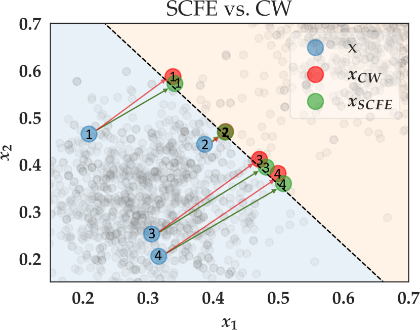
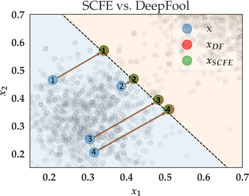
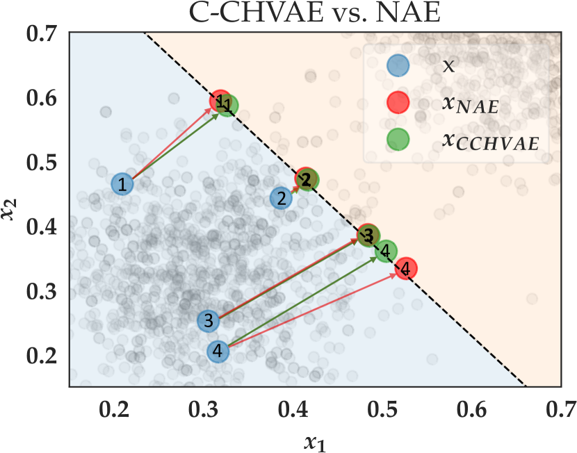
Figure 1: Similarity comparison of adversarial example and counterfactual explanation methods. Based on synthetic data, we generate adversarial examples (in red) and counterfactual explanations (in green) for some randomly chosen test set points (in blue) using methods described in Sec. 3. (Left) Both SCFE (in green) and C&W (in red) samples are close to each other, indicating strong similarity between these methods. (Middle) SCFE (in green) and DeepFool (in red) samples exactly coincide, indicating equivalence. (Right) C-CHVAE (in green) and NAE (in red) samples are closer if the blue factual points are closer to the boundary.

5 Experimental Evaluation

We now present the empirical analysis to demonstrate the similarities between counterfactual explanations and adversarial examples. More specifically, we verify the validity of our theoretical upper bounds using real-world datasets and determine the extent to which counterfactual explanations and adversarial examples similar to each other.

5.1 Experimental Setup

We first describe the synthetic and real-world datasets used to study the connections between counterfactual explanations and adversarial examples, and then we outline our experimental setup.

Synthetic Data. We generate $5000$ samples from a mixture of Gaussians with pdfs $\mathcal{N}(\mu_{1}{=}[1.0,1.0],\Sigma_{1}{=}\textbf{I})$ and $\mathcal{N}(\mu_{2}{=}[-1.0,-1.0],\Sigma_{2}{=}\textbf{I})$.

Real-world Data. We use three datasets in our experiments. 1) The UCI Adult dataset [11] consisting of $48842$ individuals with demographic (e.g., age, race, and gender), education (degree), employment (occupation, hours-per-week), personal (marital status, relationship), and financial (capital gain/loss) features. The task is to predict whether an individual’s income exceeds $\$50\text{K}$ per year or not. 2) The COMPAS dataset [25] comprising of 10000 individuals representing defendants released on bail. The task is to predict whether to release a defendant on bail or not using features, such as criminal history, jail, prison time, and defendant’s demographics. 3) The German Credit dataset from the UCI repository [11] consisting of demographic (age, gender), personal (marital status), and financial (income, credit duration) features from $1000$ credit applications. The task is to predict whether an applicant qualifies for credit or not.

Methods. Following our analysis in Sec. 4, we compare the following pair of methods: i) SCFE [40] vs. C&W [8], ii) SCFE vs. DeepFool [26], and iii) C-CHVAE [27] vs. NAE [41].

Prediction Models. For the synthetic dataset, we train a logistic regression model (LR) to learn the mixture component (samples and corresponding decision boundary shown in Fig. 1), whereas for real-world datasets, we obtain adversarial examples and counterfactuals using LR and artificial neural network (ANN) models. See Appendix C for more details.

Implementation Details For all real-world data, adversarial examples and counterfactuals are generated so as to flip the target prediction label from unfavorable ($y{=}0$) to favorable ($y{=}1$). We use $\ell_{2}$-norm as the distance function in all our experiments. We partition the dataset into train-test splits where the training set is used to train the predictor models. Adversarial examples and counterfactuals are generated for the trained models using samples in the test splits. For counterfactual explanation methods applied to generate recourse, all features are assumed actionable for fair comparison with adversarial example generation methods. See Appendix C for more implementation details.

5.2 Results

Validating our Theoretical Upper Bounds. We empirically validate the theoretical upper bounds obtained in Sec. 4. To this end, we first estimate the bounds for each instance in the test set according to Theorems 1 and 2, and compare them with the empirical estimates of the $\ell_{2}$-norm differences (LHS of Theorems 1 and 2). We use the same procedure to validate the bounds from Lemma 3.

SCFE vs. C&W and DeepFool. In Fig. 2, we show the empirical evaluation of our theoretical bounds for all real-world datasets. For each dataset, we show four box-plots: empirical estimates (green) and theoretical upper bounds (blue) of the distance ($\ell_{2}$-norm) between the resulting counterfactuals and adversarial examples for SCFE and C&W (labeled as SCFE vs. CW), and SCFE and DeepFool (labeled as SCFE vs. DF). Across all three datasets, we observe that no bounds were violated for both theorems. The gap between empirical and theoretical values is relatively small for German credit dataset as compared to COMPAS and Adult datasets. From Theorems 1 and 2, we see that the bound strongly depends on the norm of the logit score gradient $w{=}\nabla_{x}f({\mathbf{x}})$, e.g., for Adult dataset these norms are relatively higher leading to less tight bounds.

C-CHVAE vs.NAE. In Fig. 3, we validate the bounds obtained in Lemma 3 for all three datasets using an encoder-decoder framework. We observe that our upper bounds are tight, thus validating our theoretical analysis for comparing manifold-based counterfactual explanation (C-CHVAE) and adversarial example generation method (NAE).

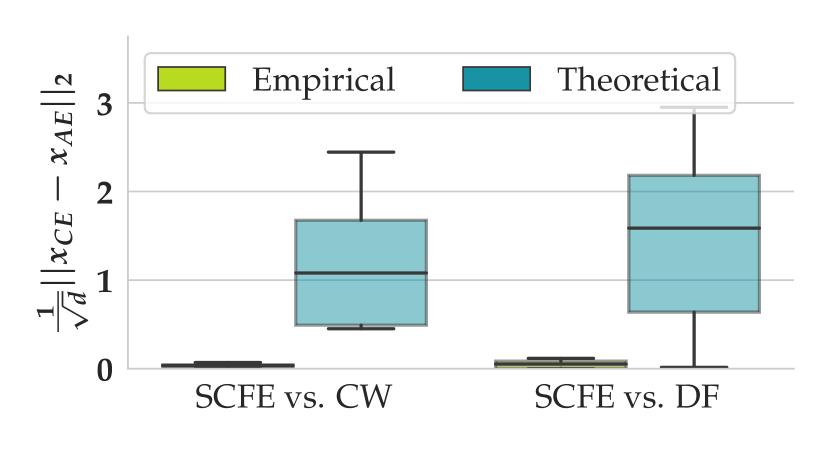
(a) Adult – LR

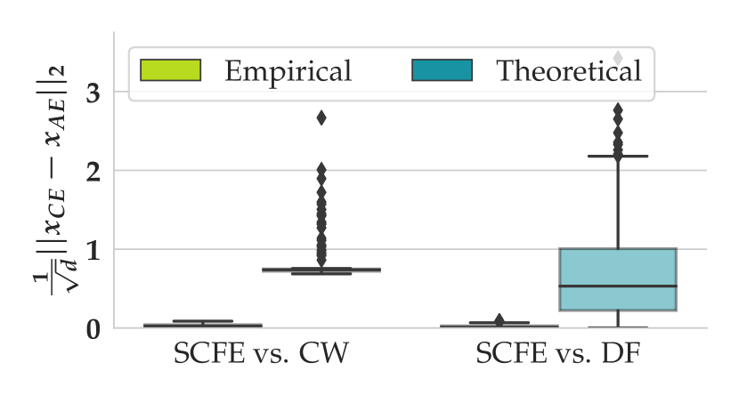
(b) COMPAS – LR

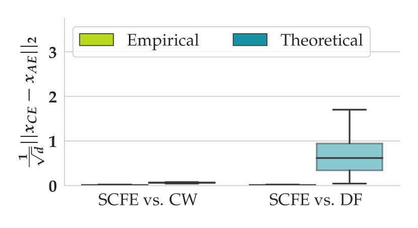
(c) German Credit – LR

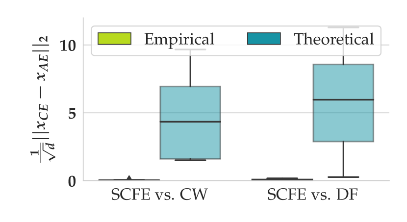
(d) Adult – ANN

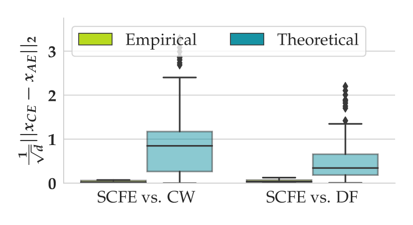
(e) COMPAS – ANN

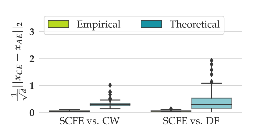
(f) German Credit – ANN

Figure 2: Verifying the theoretical bounds from Theorems 1 and 2. The green boxplots correspond to the empirical norm differences between SCFE (i.e., $x_{\text{CE}}$) and CW or DF (i.e., $x_{\text{AE}}$). The blue boxplots show the distribution of upper bounds, which we evaluated by plugging in the necessary quantities (hyperparameters, gradients, logit values) into equations 7 and 8. No bounds are violated. For ANNs, the upper bounds were computed using local linear model approximations.

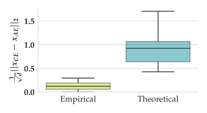
(a) Adult – ANN

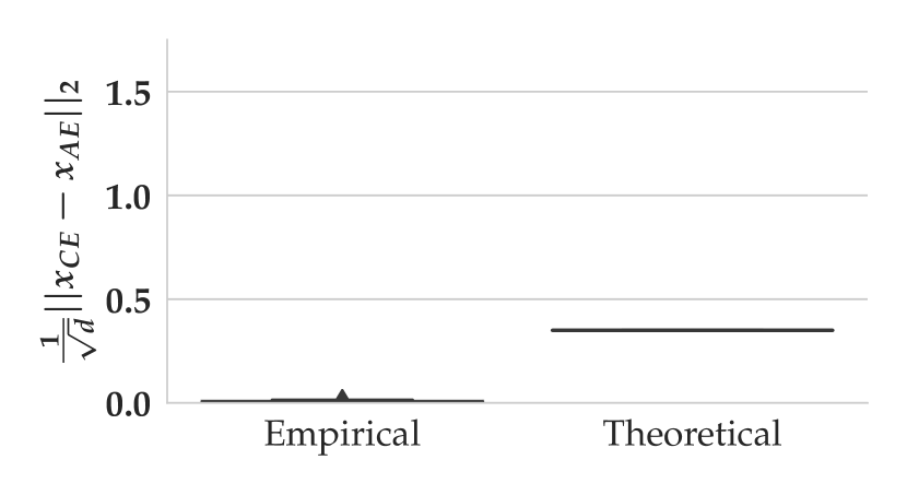
(b) COMPAS – ANN

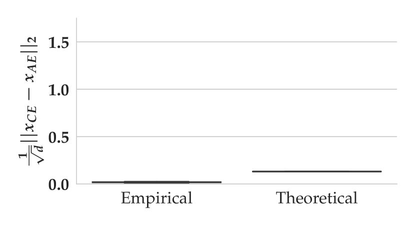
(c) German Credit – ANN

Figure 3: Verifying the theoretical bounds from Lemma 2. The green boxplots correspond to the empirical norm differences between CCHVAE (i.e., $x_{\text{CE}}$) and NAE (i.e., $x_{\text{AE}}$). The blue boxplots show the distribution of upper bounds, which we evaluated by plugging in the corresponding quantities (hyperparameters, Lipschitz constant) into the upper bound from Lemma 2. The Lipschitz constant is computed based on decoders and encoders using Lemma 4. No bounds are violated.

Similarities between Counterfactuals and Adversarial examples. Here, we qualitatively and quantitatively show the similarities between counterfactuals and adversarial examples using several datasets.

Analysis with Synthetic Data. In Fig. 1, we show the similarity between counterfactual explanations and adversarial examples generated for a classifier trained on a two-dimensional mixture of Gaussian datasets. Across all cases, we observe that most output samples generated by counterfactual explanation and adversarial example methods overlap. In particular, for samples near the decision boundary, the solutions tend to be more similar. These results confirm our theoretical bounds, which depend on the difference between the logit sample prediction $f({\mathbf{x}})$ and the target score $s$. If points are close to the decision boundary, $f({\mathbf{x}})$ is closer to $s$, suggesting that the resulting counterfactual and adversarial example will be closer as implied by Theorems 1 and 2.

Table 1: Average Spearman rank correlation between counterfactual and adversarial perturbations. For every input ${\mathbf{x}}$, we compute the corresponding adversarial perturbation $\delta_{\text{AE}}$ and the counterfactual perturbation $\delta_{\text{CE}}$. We then compute Spearman’s $\rho(\delta_{\text{AE}},\delta_{\text{CE}})$ and report their means (gradient-based: (g); manifold-based: (m)).

	COMPAS				Adult
	LR		ANN		LR		ANN
Model	SCFE (g)	CCHVAE (m)	SCFE (g)	CCHVAE (m)	SCFE (g)	CCHVAE (m)	SCFE (g)	CCHVAE (m)
CW (g)	$0.88\pm 0.16$	$0.67\pm 0.30$	$0.93\pm 0.10$	$0.67\pm 0.22$	$\mathbf{0.95\pm 0.06}$	$0.86\pm 0.10$	$0.92\pm 0.09$	$0.70\pm 0.16$
DF (g)	$\mathbf{0.91\pm 0.12}$	$0.68\pm 0.31$	$\mathbf{0.97\pm 0.03}$	$0.65\pm 0.22$	$0.92\pm 0.06$	$0.80\pm 0.13$	$\mathbf{0.93\pm 0.08}$	$0.63\pm 0.20$
NAE (m)	$0.57\pm 0.35$	$\mathbf{0.94\pm 0.08}$	$0.71\pm 0.19$	$\mathbf{1.00\pm 0.00}$	$0.83\pm 0.12$	$\mathbf{0.90\pm 0.10}$	$0.74\pm 0.13$	$\mathbf{0.98\pm 0.02}$

Analysis with Real Data. For real-world datasets, we define two additional metrics beyond those studied in our theoretical analysis to gain a more granular understanding about the similarities of counterfactuals and adversarial examples. First, we introduce $d_{\text{match}}$ which quantifies the similarity between counterfactuals (i.e., ${\mathbf{x}}_{\text{CE}}$) and adversarial examples (i.e., ${\mathbf{x}}_{\text{AE}}$):

$$d_{\text{match}} =\frac{1}{n}\sum_{i=1}^{n}\mathbbm{1}\bigg{[}\frac{1}{\sqrt{d}}\lVert{\mathbf{x}}_{\text{CE}}^{(i)}-{\mathbf{x}}_{\text{AE}}^{(i)}\rVert_{2}<\theta\bigg{]},$$ (12)

where $n$ is the total number of instances used in the analysis and $\theta{\in}\{0.02,0.05,0.1\}$ is a threshold determining when to consider counterfactual and adversarial examples as equivalent. $d_{\text{match}}$ evaluates whether counterfactuals and adversarial examples are exactly the same with higher $d_{\text{match}}$ implying higher similarity. Second, we complement $d_{\text{match}}$ by Spearman rank $\rho$ between $\delta_{\text{CE}}$ and $\delta_{\text{AE}}$, which is a rank correlation coefficient measuring to what extent the perturbations’ rankings agree, i.e., whether adversarial example generation methods and counterfactual explanation methods deem the same dimensions important in order to arrive at their final outputs. Here, $\rho(\delta_{\text{CE}},\delta_{\text{AE}}){=}1$ implies that the rankings are same, $0$ suggests that the rankings are independent, and $-1$ indicates reversely ordered rankings.

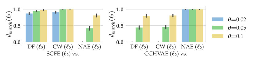
(a) COMPAS

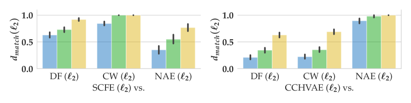
(b) Adult

Figure 4: Analyzing to what extent different counterfactual explanation methods and adversarial example generation methods are empirically equivalent for the logistic regression classifier. To do that, we compute $d_{\text{match}}$ from Eqn. 12. Missing bars indicate that there was no match.

In Fig. 4, we compare a given counterfactual explanation method to salient adversarial example generation methods (DeepFool, C&W, and NAE) using $d_{\text{match}}$. We show the results for Adult and COMPAS datasets using LR models and relegate results for German Credit as well as neural network classifiers to Appendix D. Our results in Fig. 4 validate that the SCFE method is similar to DeepFool and C&W (higher $d_{\text{match}}$ for lower $\theta$). Across all datasets, this result aligns and validates with the similarity analysis in Sec. 4. Similarly, manifold-based methods demonstrate higher $d_{\text{match}}$ compared to non-manifold methods (right panels in Fig. 4). Additionally, we show the results from the rank correlation analysis in Table 1 and observe that the maximum rank correlations (between 0.90 and 1.00) are obtained for methods that belong to the same categories, suggesting that the considered counterfactuals and adversarial examples are close to being equivalent.

6 Conclusion

In this work, we formally analyzed the connections between state-of-the-art adversarial example generation methods and counterfactual explanation methods. To this end, we first highlighted salient counterfactual explanation and adversarial example methods in literature, and leveraged similarities in their objective functions, optimization algorithms and constraints utilized in these methods to theoretically analyze conditions for equivalence and bound the distance between the solutions output by counterfactual explanation and adversarial example generation methods. For locally linear models, we bound the distance between the solutions obtained by C&W and SCFE using loss functions preferred in the respective works. We obtained similar bounds for the solutions of DeepFool and SCFE. We also demonstrated equivalence between the manifold-based methods of NAE and C-CHVAE and bounded the distance between their respective solutions. Finally, we empirically evaluated our theoretical findings on simulated and real-world data sets.

By establishing theoretically and empirically that several popular counterfactual explanation algorithms are generating extremely similar solutions as those of well known adversarial example algorithms, our work raises fundamental questions about the design and development of existing counterfactual explanation algorithms. Do we really want counterfactual explanations to resemble adversarial examples, as our work suggests they do? How can a decision maker distinguish an adversarial attack from a counterfactual explanation? Does this imply that decision makers are tricking their own models by issuing counterfactual explanations? Can we do a better job of designing counterfactual explanations? Moreover, by establishing connections between popular counterfactual explanation and adversarial example algorithms, our work opens up the possibility of using insights from adversarial robustness literature to improve the design and development of counterfactual explanation algorithms.

We hope our formal analysis helps carve a path for more robust approaches to counterfactual explanations, a critical aspect for calibrating trust in ML. Improving our theoretical bounds using other strategies and deriving new theoretical bounds for other approaches is an interesting future direction.

Appendix Summary

Section A provides a categorization of counterfactual explanation and adversarial example methods. In Section B, we provide detailed proofs for Lemmas 1 and 3, and Theorems 1 and 2. In Section C, we provide implementation details for all models used in our experiments including (i) the supervised learning models, (ii) the counterfactual explanation and adversarial example methods, and the (iii) generative models required to run the manifold-based methods. Finally, in Section D, we present the remaining experiments we referred to in the main text.

Appendix A Taxonomy of Counterfactual and Adversarial Example Methods

In order to choose methods to compare across counterfactual explanation methods and adversarial example generation methods, we surveyed existing literature. We use a taxonomy to categorize each subset of methods based on various factors. The main characteristics we use are based on type of method, based on widely accepted terminology and specific implementation details. In particular, we distinguish between i) constraints imposed for generating adversarial examples or counterfactual explanations, ii) algorithms used for generating them. For the class of adversarial example generation methods, we further distinguish between poisoning attacks and evasion attacks and note that evasion attacks are most closely related to counterfactual explanation methods. The taxonomy for counterfactual explanation methods is provided in Table 2 and that for adversarial example generation methods is provided in Table 3.

The main algorithm types used for counterfactual explanation methods are search-based, gradient-based and one method that uses integer programming [36]. The main constraints considered are actionability i.e., only certain features are allowed to change, and counterfactual explanations are encouraged to be realistic using either causal and/or manifold constraints. Similarly, for adversarial example generation methods primarily, Greedy search-based and gradient-based methods are most common. Manifold constraints are also imposed in a few cases where the goal is to generate adversaries close to the data-distribution. Based on this taxonomy, we select the appropriate pairs of counterfactual explanation method and adversarial example generation method to compare to each other for theoretical analysis. This leads us to compare gradient-based methods SCFE and C&W attack, SCFE and DeepFool and finally, manifold-based methods C-CHVAE and NAE with their search-based algorithms.

Table 2: Taxonomy of counterfactual explanation methods

Algorithm	Constraints	Method
Search-based	Causal, Actionability Manifold, Actionability	MINT [20] C-CHVAE [27]
Gradient-based	Actionability Manifold, Actionability	CFE, SCFE [40] REVISE [17]
Integer-programming	Actionability/Linear black-box	AR [36]

Table 3: Taxonomy of adversarial example generation methods

	Algorithm	Constraints	Method
Poisoning Attacks	Greedy Search	Manifold	Adv. Data Poisoning [35]
	Gradient-based	Data-domain	SVM-attack [5]
			One-Shot Kill [31]
Evasion Attacks	Search-based	Manifold	NAE [41]
	Gradient-based	Data-domain	DeepFool [26]
			C&W Attack [8]

Appendix B Proofs for Section 4

B.1 Proof of Lemma 1

Lemma 1.

For a linear score function $f(x)={\mathbf{w}}^{\top}{\mathbf{x}}+b$, the SCFE counterfactual for ${\mathbf{x}}$ on $f$ is ${\mathbf{x}}^{\prime}={\mathbf{x}}+\delta^{*}$ where

$$\delta^{*}=(\mathbf{{\mathbf{w}}{\mathbf{w}}^{T}}+\lambda\mathbf{I})^{-1}(s-\mathbf{w}^{T}\mathbf{x}-b){\mathbf{w}}.$$

Proof.

Reformulating Equation 1 using $l_{2}$-norm as the distance metric, we get:

$$\min_{\mathbf{x^{\prime}}}(\mathbf{w}^{T}\mathbf{x^{\prime}}+b-s)^{2}+\lambda||\mathbf{x^{\prime}}-\mathbf{x}||_{2}^{2}.$$

We can convert this minimization objective into finding the minimum perturbation $\delta$ by substituting $\mathbf{x^{\prime}}=\mathbf{x}+\delta$, i.e.,

$$\min_{\delta}(\mathbf{w}^{T}\mathbf{x}+\mathbf{w}^{T}\delta+b-s)^{2}+\lambda||\mathbf{x}^{\prime}-\mathbf{x}||_{2}^{2}.$$ (13)

Using $s-\mathbf{w}^{T}\mathbf{x}-b=m$ as a dummy variable and $\mathbf{x}^{\prime}-\mathbf{x}=\delta$, we get:

$$\min_{\delta}(\mathbf{w}^{T}\delta-m)^{2}+\lambda||\delta||_{2}^{2}$$

$$\min_{\delta}(\mathbf{w}^{T}\delta-m)^{T}(\mathbf{w}^{T}\delta-m)+\lambda\delta^{T}\delta$$

$$\min_{\delta}(\delta^{T}\mathbf{w}-m)(\mathbf{w}^{T}\delta-m)+\lambda\delta^{T}\delta m m^{T}=m$$ ( is a scalar, hence )

$$\min_{\delta}\delta^{T}\mathbf{w}\mathbf{w}^{T}\delta-2m\delta^{T}\mathbf{w}+m^{2}+\lambda\delta^{T}\delta$$

$$\min_{\delta}\delta^{T}(\mathbf{w}\mathbf{w}^{T}+\lambda\mathbf{I})\delta-2m\delta^{T}\mathbf{w}+m^{2}$$

$$\min_{\delta}\delta^{T}\mathbf{M}\delta-2m\mathbf{w}^{T}\delta+m^{2} \mathbf{M}=\mathbf{w}\mathbf{w}^{T}+\lambda\mathbf{I}$$ (where )

$$\min_{\delta}\delta^{T}\mathbf{M}\delta-2\eta^{T}\delta+m^{2} m\mathbf{w}=\eta$$ (where )

$$\min_{\delta}\delta^{T}\mathbf{M}\delta-2\eta^{T}\delta+\eta^{T}\mathbf{M}^{-1}\eta-\eta^{T}\mathbf{M}^{-1}\eta+m^{2}$$

$$\min_{\delta}(\delta-\mathbf{M}^{-1}\eta)^{T}\mathbf{M}(\delta-\mathbf{M}^{-1}\eta)-\eta^{T}\mathbf{M}^{-1}\eta+m^{2}$$

The closed form solution is given by,

$$\delta^{*}=\mathbf{M}^{-1}\eta,$$ (14)

where $M={\mathbf{w}}{\mathbf{w}}^{T}+\lambda\mathbf{I}$.

The expression in (14) can further be simplified:

$$\delta^{*} =m\bigg{(}\mathbf{I}-\frac{{\mathbf{w}}{\mathbf{w}}^{T}}{\lambda+\lVert{\mathbf{w}}\rVert_{2}^{2}}\bigg{)}{\mathbf{w}} (\text{Sherman-Morrison Formula})$$

$$=m\bigg{(}\mathbf{I}{\mathbf{w}}-{\mathbf{w}}\frac{\lVert{\mathbf{w}}\rVert_{2}^{2}}{\lambda+\lVert{\mathbf{w}}\rVert_{2}^{2}}\bigg{)}$$

$$=m\cdot\frac{\lambda}{\lambda+\lVert{\mathbf{w}}\rVert_{2}^{2}}\cdot{\mathbf{w}},$$ (15)

where $m:=s-{\mathbf{w}}^{T}{\mathbf{x}}-b$. We can also solve for the optimal hyperparamter $\lambda$:

$$s =b+{\mathbf{w}}^{T}(x+\delta^{*}) \delta^{*} s$$ ( leads to target )

$$=b+{\mathbf{w}}^{T}x+{\mathbf{w}}^{T}\delta^{*}$$

$$\iff m ={\mathbf{w}}^{T}\delta^{*}$$

$$\Rightarrow m =m\cdot\frac{\lambda\cdot\lVert{\mathbf{w}}\rVert_{2}^{2}}{\lambda+\lVert{\mathbf{w}}\rVert_{2}^{2}}$$ (insert (15))

$$\lambda^{*} =\frac{\lVert{\mathbf{w}}\rVert_{2}^{2}}{\lVert{\mathbf{w}}\rVert_{2}^{2}-1}$$

Notice, that the optimal hyperparameter can also be negative, if $0<\lVert{\mathbf{w}}\rVert_{2}^{2}<1$! Finally, substituting into (15) yields:

$$\delta^{**}=\frac{m}{\lVert{\mathbf{w}}\rVert_{2}^{2}}\cdot{\mathbf{w}}.$$ (16)

∎

B.2 Proof of Lemma 3

Lemma 3.

For a binary classifier $h({\mathbf{x}})=g(f({\mathbf{x}}))$ such that $f({\mathbf{x}})={\mathbf{w}}^{\top}{\mathbf{x}}+b$, $g({\mathbf{x}})=\sigma({\mathbf{x}})$, and $h({\mathbf{x}})$ is the probability that ${\mathbf{x}}$ is in the class $y=1$,

$$\ell^{*}({\mathbf{x}})=\max(0,-2({\mathbf{w}}^{\top}{\mathbf{x}}+b))$$

.

Proof.

Given our formulation of $h({\mathbf{x}})$, $f({\mathbf{x}})$ is the score corresponding to class $y=1$. By the definition of $\sigma({\mathbf{x}})$,

$$f({\mathbf{x}})=\ln{\frac{h({\mathbf{x}})}{1-h({\mathbf{x}})}}=\ln{h({\mathbf{x}})}-\ln{(1-h({\mathbf{x}}))}$$

Then the score corresponding to the class $y=0$ is

$$\ln{\frac{1-h({\mathbf{x}})}{1-(1-h({\mathbf{x}}))}}=\ln{\frac{1-h({\mathbf{x}})}{h({\mathbf{x}})}}=\ln{(1-h({\mathbf{x}}))}-\ln{h({\mathbf{x}})}=-f({\mathbf{x}})$$

Substituting back into definition of $\ell^{*}({\mathbf{x}})$,

$$\ell^{*}({\mathbf{x}}) =\max(0,\max_{i}(f({\mathbf{x}})_{i})-f({\mathbf{x}})_{y})$$

$$=\max(0,(-f({\mathbf{x}})-f({\mathbf{x}}))$$

$$=\max(0,(-2f({\mathbf{x}}))$$

$$=\max(0,-2({\mathbf{w}}^{\top}{\mathbf{x}}+b)).$$

∎

B.3 Proof of Theorem 1

Theorem 1.

For a linear classifier $h({\mathbf{x}})=g(f({\mathbf{x}}))$ such that $f({\mathbf{x}})={\mathbf{w}}^{T}{\mathbf{x}}+b$, the difference between the SCFE counterfactual example $\mathbf{x}_{\text{SCFE}}$ and the C&W adversarial example $\mathbf{x}_{\text{CW}}$ using the recommended loss function $\ell^{*}(\cdot)=\max(0,\max_{i}(f({\mathbf{x}})_{i})-f({\mathbf{x}})_{y})$ is given by:

$$\lVert\mathbf{x}_{\text{SCFE}}-\mathbf{x}_{\text{CW}}\rVert_{p}\leq\biggl{\lVert}\frac{1}{\lambda}\bigg{(}\mathbf{I}-\frac{\mathbf{w}\mathbf{w}^{T}}{\lambda+\mathbf{w}^{T}\mathbf{w}}\bigg{)}(s-f(\mathbf{x}))-c\mathbf{I}\biggr{\rVert}_{p}\leavevmode\nobreak\ \lVert\mathbf{w}\rVert_{p}$$

.

Proof.

Consider a binary classifier $h({\mathbf{x}})=g(f({\mathbf{x}}))$ such that $f({\mathbf{x}})={\mathbf{w}}^{\top}{\mathbf{x}}+b$, $g({\mathbf{x}})=\sigma({\mathbf{x}})$, and $h({\mathbf{x}})$ is the probability that ${\mathbf{x}}$ is in the class $y=1$. Then by Lemma 3 and using $\ell_{2}$-nrom as the distance metric, we can write the C&W Attack objective as

$$\arg\min_{{\mathbf{x}}^{\prime}}c\max(0,-2({\mathbf{w}}^{\top}{\mathbf{x}}^{\prime}+b))+\lVert{\mathbf{x}}-{\mathbf{x}}^{\prime}\rVert_{2}^{2}$$

We can convert this minimization objective into finding the minimum perturbation $\delta$ by substituting $\mathbf{x^{\prime}}=\mathbf{x}+\delta$,

$$\arg\min_{\delta}c\max(0,-2({\mathbf{w}}^{\top}{\mathbf{x}}+{\mathbf{w}}^{\top}\delta+b))+\lVert\delta\rVert_{2}^{2}$$

The subgradients of this objective are

$$\begin{cases}2\delta&\mbox{when }-2({\mathbf{w}}^{\top}{\mathbf{x}}+{\mathbf{w}}^{\top}\delta+b)<0\\ -2c{\mathbf{w}}+2\delta&\mbox{otherwise}\end{cases}$$

By Lemma 3, $-2({\mathbf{w}}^{\top}{\mathbf{x}}+{\mathbf{w}}^{\top}\delta+b)=-f({\mathbf{x}})-f({\mathbf{x}})<0$. This implies that $f({\mathbf{x}})>-f({\mathbf{x}})$, i.e that the score for class $y=1$ is greater than the score for $y=0$. As this indicates an adversarial example has already been found, we focus on minimizing the other subgradient. Setting this subgradient equal to 0,

$$0 =-2c{\mathbf{w}}+2\delta$$

$$\delta =c{\mathbf{w}}$$

Thus the minimum perturbation to generate and adversarial example using the C&W Attack is

$$\delta_{\text{CW}}^{*}=c{\mathbf{w}}$$

Now, taking the difference between the minimum perturbation to generate a SCFE counterfactual (Lemma 1) and DeepFool ((18)), we get:

$$\delta^{*}_{\text{SCFE}}-\delta^{*}_{\text{CW}} =(\mathbf{w}\mathbf{w}^{T}+\lambda\mathbf{I})^{-1}(s-\mathbf{w}^{T}\mathbf{x}-b)\mathbf{w}-c{\mathbf{w}}$$

$$=\big{(}(\mathbf{w}\mathbf{w}^{T}+\lambda\mathbf{I})^{-1}(s-f({\mathbf{x}}))-c\mathbf{I}\big{)}{\mathbf{w}}$$

$$=\bigg{(}\frac{1}{\lambda}\bigg{(}\mathbf{I}-\frac{\mathbf{w}\mathbf{w}^{T}}{\lambda+\mathbf{w}^{T}\mathbf{w}}\bigg{)}(s-f(\mathbf{x}))-c\mathbf{I}\bigg{)}\mathbf{w}$$ (Using Sherman–Morrison formula)

Taking the $l_{p}$-norm on both sides, we get:

$$\lVert\delta^{*}_{\text{SCFE}}-\delta^{*}_{\text{CW}}\rVert_{p} =\biggl{\lVert}\bigg{(}\frac{1}{\lambda}\bigg{(}\mathbf{I}-\frac{\mathbf{w}\mathbf{w}^{T}}{\lambda+\mathbf{w}^{T}\mathbf{w}}\bigg{)}(s-f(\mathbf{x}))-c\mathbf{I}\bigg{)}\mathbf{w}\biggr{\rVert}_{p}$$

$$\leq\biggl{\lVert}\frac{1}{\lambda}\bigg{(}\mathbf{I}-\frac{\mathbf{w}\mathbf{w}^{T}}{\lambda+\mathbf{w}^{T}\mathbf{w}}\bigg{)}(s-f(\mathbf{x}))-c\mathbf{I}\biggr{\rVert}_{p}\leavevmode\nobreak\ \lVert\mathbf{w}\rVert_{p}$$ (Using Cauchy-Schwartz)

Adding and subtracting the input instance $\mathbf{x}$ in the left term, we get:

$$\|\mathbf{x}+\delta^{*}_{\text{SCFE}}-(\mathbf{x}+\delta^{*}_{\text{CW}})\|_{p} \leq\biggl{\lVert}\frac{1}{\lambda}\bigg{(}\mathbf{I}-\frac{\mathbf{w}\mathbf{w}^{T}}{\lambda+\mathbf{w}^{T}\mathbf{w}}\bigg{)}(s-f(\mathbf{x}))-c\mathbf{I}\biggr{\|}_{p}\leavevmode\nobreak\ \lVert\mathbf{w}\rVert_{p}$$

$$\lVert\mathbf{x}_{\text{SCFE}}-\mathbf{x}_{\text{CW}}\rVert_{p} \leq\biggl{\lVert}\frac{1}{\lambda}\bigg{(}\mathbf{I}-\frac{\mathbf{w}\mathbf{w}^{T}}{\lambda+\mathbf{w}^{T}\mathbf{w}}\bigg{)}(s-f(\mathbf{x}))-c\mathbf{I}\biggr{\|}_{p}\leavevmode\nobreak\ \|\mathbf{w}\|_{p},$$

where the final equation gives an upper bound on the difference between the SCFE counterfactual and the C&W adversarial example.

Furthermore, we ask under which conditions the normed difference becomes 0. We start with:

$$\delta^{*}_{\text{SCFE}}-\delta^{*}_{\text{CW}} =m\cdot\frac{\lambda}{\lambda+\lVert{\mathbf{w}}\rVert_{2}^{2}}\cdot{\mathbf{w}}-c\cdot{\mathbf{w}}$$

Taking the $l_{p}$-norm on both sides, we get:

$$\lVert\delta^{*}_{\text{SCFE}}-\delta^{*}_{\text{CW}}\rVert_{p} =\biggl{|}m\cdot\frac{\lambda}{\lambda+\lVert{\mathbf{w}}\rVert_{2}^{2}}-c\biggr{|}\cdot\lVert{\mathbf{w}}\|_{p}$$

If we were to use the optimal hyperparameters we would get:

$$\lVert\delta^{**}_{\text{SCFE}}-\delta^{*}_{\text{CW}}\rVert_{p}=\biggl{|}\frac{m-c\cdot\lVert{\mathbf{w}}\rVert_{2}^{2}}{\lVert{\mathbf{w}}\rVert_{2}^{2}}\biggr{|}\cdot\lVert{\mathbf{w}}\rVert_{p},$$

where equality holds when the hyperparameter is chosen so that $c:=\frac{m}{\lVert{\mathbf{w}}\rVert_{2}^{2}}.$ ∎

B.4 Proof of Theorem 2

Theorem 2.

For a linear classifier $h({\mathbf{x}})=g(f({\mathbf{x}}))$ such that $f({\mathbf{x}})={\mathbf{w}}^{T}{\mathbf{x}}+b$, the difference between the counterfactual example $\mathbf{x}_{\text{SCFE}}$ generated by Wachter et al. [40] and the adversarial example $\mathbf{x}_{\text{DF}}$ generated by Moosavi-Dezfooli et al. [26] is given by:

$$||\mathbf{x}_{\text{SCFE}}-\mathbf{x}_{\text{DF}}||_{p}\leq\biggl{\lVert}\frac{1}{\lambda}\bigg{(}\mathbf{I}-\frac{\mathbf{w}\mathbf{w}^{T}}{\lambda+\mathbf{w}^{T}\mathbf{w}}\bigg{)}(s-f(\mathbf{x}))+\bigg{(}{\mathbf{I}}\frac{f(\mathbf{x})}{\lVert\mathbf{w}\rVert_{2}^{2}}\bigg{)}\biggr{\rVert}_{p}\leavevmode\nobreak\ \cdot||\mathbf{w}||_{p},$$ (17)

Proof.

The minimal perturbation to change the classifier’s decision for a binary model $f(\mathbf{x})$ is given by the closed-form formula [26]:

$$\delta^{*}_{\text{DF}}=-\frac{f(\mathbf{x})}{||\mathbf{w}||_{2}^{2}}\mathbf{w}.$$ (18)

Now, taking the difference between the minimum perturbation added to an input instance $\mathbf{x}$ by Wachter algorithm (Lemma 1) and DeepFool ((18)), we get:

$$\delta^{*}_{\text{SCFE}}-\delta^{*}_{\text{DF}}=(\mathbf{w}\mathbf{w}^{T}+\lambda\mathbf{I})^{-1}(s-\mathbf{w}^{T}\mathbf{x}-b)\mathbf{w}-\bigg{(}-\frac{f(\mathbf{x})}{||\mathbf{w}||_{2}^{2}}\mathbf{w}\bigg{)}$$

$$\delta^{*}_{\text{SCFE}}-\delta^{*}_{\text{DF}}=\bigg{(}(\mathbf{w}\mathbf{w}^{T}+\lambda\mathbf{I})^{-1}(s-f(\mathbf{x}))+\frac{f(\mathbf{x})}{||\mathbf{w}||_{2}^{2}}\bigg{)}\mathbf{w}$$

$$\delta^{*}_{\text{SCFE}}-\delta^{*}_{\text{DF}}=\bigg{(}\frac{1}{\lambda}\bigg{(}\mathbf{I}-\frac{\mathbf{w}\mathbf{w}^{T}}{\lambda+\mathbf{w}^{T}\mathbf{w}}\bigg{)}(s-f(\mathbf{x}))+\frac{f(\mathbf{x})}{||\mathbf{w}||_{2}^{2}}\bigg{)}\mathbf{w}$$ (Using Sherman–Morrison formula)

Taking the $l_{p}$-norm on both sides, we get:

$$\lVert\delta^{*}_{\text{SCFE}}-\delta^{*}_{\text{DF}}\|_{p} =\biggl{\|}\bigg{(}\frac{1}{\lambda}\bigg{(}\mathbf{I}-\frac{\mathbf{w}\mathbf{w}^{T}}{\lambda+\mathbf{w}^{T}\mathbf{w}}\bigg{)}(s-f(\mathbf{x}))+{\mathbf{I}}\frac{f(\mathbf{x})}{\|\mathbf{w}\|_{2}^{2}}\bigg{)}\mathbf{w}\biggr{\|}_{p}$$

$$\leq\biggl{\|}\frac{1}{\lambda}\bigg{(}\mathbf{I}-\frac{\mathbf{w}\mathbf{w}^{T}}{\lambda+\mathbf{w}^{T}\mathbf{w}}\bigg{)}(s-f(\mathbf{x}))+{\mathbf{I}}\frac{f(\mathbf{x})}{\|\mathbf{w}\|_{2}^{2}}\biggr{\|}_{p}\leavevmode\nobreak\ \|\mathbf{w}\|_{p}$$ (Using Cauchy-Schwartz)

Adding and subtracting the input instance $\mathbf{x}$ in the left term, we get:

$$\|\mathbf{x}+\delta^{*}_{\text{SCFE}}-(\mathbf{x}+\delta^{*}_{\text{DF}})\|_{p} \leq\biggl{\|}\frac{1}{\lambda}\bigg{(}\mathbf{I}-\frac{\mathbf{w}\mathbf{w}^{T}}{\lambda+\mathbf{w}^{T}\mathbf{w}}\bigg{)}(s-f(\mathbf{x}))+{\mathbf{I}}\frac{f(\mathbf{x})}{\|\mathbf{w}\|_{2}^{2}}\biggr{\|}_{p}\leavevmode\nobreak\ \|\mathbf{w}\|_{p}$$

$$\|\mathbf{x}_{\text{SCFE}}-\mathbf{x}_{\text{DF}}\|_{p} \leq\biggl{\|}\frac{1}{\lambda}\bigg{(}\mathbf{I}-\frac{\mathbf{w}\mathbf{w}^{T}}{\lambda+\mathbf{w}^{T}\mathbf{w}}\bigg{)}(s-f(\mathbf{x}))+{\mathbf{I}}\frac{f(\mathbf{x})}{\|\mathbf{w}\|_{2}^{2}}\biggr{\|}_{p}\leavevmode\nobreak\ \|\mathbf{w}\|_{p},$$

where the final equation gives an upper bound on the difference between the SCFE counterfactual and the adversarial example from DeepFool [26].

Furthermore, we ask under which conditions the normed difference becomes 0.

$$\delta^{*}_{\text{SCFE}}-\delta^{*}_{\text{DF}} =m\cdot\frac{\lambda}{\lambda+\lVert{\mathbf{w}}\rVert_{2}^{2}}\cdot{\mathbf{w}}+\frac{f(\mathbf{x})}{\|\mathbf{w}\|_{2}^{2}}\mathbf{w}$$

$$=\frac{m\cdot\lambda\cdot\lVert{\mathbf{w}}\rVert_{2}^{2}+f({\mathbf{x}})\cdot(\lambda+\lVert{\mathbf{w}}\rVert_{2}^{2})}{(\lambda+\lVert{\mathbf{w}}\rVert_{2}^{2})\cdot\lVert{\mathbf{w}}\rVert_{2}^{2}}\cdot{\mathbf{w}}$$

$$=\frac{f({\mathbf{x}})\cdot\lVert{\mathbf{w}}\rVert_{2}^{2}\cdot(1-\lambda)+\lambda\cdot(f({\mathbf{x}})+s\cdot\lVert{\mathbf{w}}\rVert_{2}^{2})}{(\lambda+\lVert{\mathbf{w}}\rVert_{2}^{2})\cdot\lVert{\mathbf{w}}\rVert_{2}^{2}}\cdot{\mathbf{w}}$$

Taking the $l_{p}$-norm on both sides and , we get:

$$\lVert\delta^{*}_{\text{SCFE}}-\delta^{*}_{\text{DF}}\rVert_{p} =\biggl{|}\frac{f({\mathbf{x}})\cdot\lVert{\mathbf{w}}\rVert_{2}^{2}\cdot(1-\lambda)+\lambda\cdot(f({\mathbf{x}})+s\cdot\lVert{\mathbf{w}}\rVert_{2}^{2})}{(\lambda+\lVert{\mathbf{w}}\rVert_{2}^{2})\cdot\lVert{\mathbf{w}}\rVert_{2}^{2}}\biggr{|}\cdot\|\mathbf{w}\|_{p}$$

If we were to use the optimal hyperparameter $\lambda^{*}$ we would get:

$$\lVert\delta^{**}_{\text{SCFE}}-\delta^{*}_{\text{DF}}\rVert_{p} =\biggl{\lVert}\frac{-f({\mathbf{x}})+s}{\lVert{\mathbf{w}}\rVert_{2}^{2}}\cdot{\mathbf{w}}+\frac{-f({\mathbf{x}})}{\lVert{\mathbf{w}}\rVert_{2}^{2}}\cdot{\mathbf{w}}\biggr{\rVert}_{p}$$

$$=\frac{|s|}{\lVert{\mathbf{w}}\rVert_{2}^{2}}\cdot\lVert{\mathbf{w}}\rVert_{p},$$

where equality holds when the target score is chosen so that $s{=}0$, which corresponds to a probability of $Y{=}1$ of $0.5$.

∎

B.5 Proof of Lemma 2

Lemma 2.

Let $\tilde{{\mathbf{z}}}_{NAE}$ be the solution returned Zhao et al. [41, Algorithm 1] and $\tilde{{\mathbf{z}}}_{C}$ the solution returned by the counterfactual search algorithm of Pawelczyk et al. [27] by sampling from $\ell_{p}$-norm ball in the latent space using an $L$-Lipschitz generative model $\mathcal{G}_{\theta}(\cdot)$. Analogously, let ${\mathbf{x}}_{NAE}=\mathcal{G}_{\theta}(\tilde{{\mathbf{z}}}_{\text{NAE}})$ and ${\mathbf{x}}_{C}=\mathcal{G}_{\theta}(\tilde{{\mathbf{z}}}_{C})$ by design of the two algorithms. Let $r_{\text{NAE}}^{*}$ and $r_{C}^{*}$ be the corresponding radius chosed by each algorithm respectively that successfully returns an adversarial example or counterfactual explanation. Then, $\|{\mathbf{x}}_{\text{NAE}}-{\mathbf{x}}_{C}\|\leq L(r_{\text{NAE}}^{*}+r_{C}^{*})$.

Proof.

The proof straightforwardly follows from triangle inequality and $L$-Lipschitzness of the Generative model:

$$\|{\mathbf{x}}_{\text{NAE}}-{\mathbf{x}}_{C}\| =\|\mathcal{G}_{\theta}(\tilde{{\mathbf{z}}}_{\text{NAE}})-\mathcal{G}_{\theta}(\tilde{{\mathbf{z}}}_{C})\|_{p}$$ (19)

$$\leq\|\mathcal{G}_{\theta}(\tilde{{\mathbf{z}}}_{\text{NAE}})-{\mathbf{x}}+{\mathbf{x}}-\mathcal{G}_{\theta}(\tilde{{\mathbf{z}}}_{C})\|_{p}$$ (20)

$$\leq\|\mathcal{G}_{\theta}(\tilde{{\mathbf{z}}}_{\text{NAE}})-{\mathbf{x}}\|_{p}+\|{\mathbf{x}}-\mathcal{G}_{\theta}(\tilde{{\mathbf{z}}}_{C})\|_{p}$$ (21)

$$=\|\mathcal{G}_{\theta}(\tilde{{\mathbf{z}}}_{\text{NAE}})-\mathcal{G}_{\theta}({\mathbf{z}})\|_{p}+\|\mathcal{G}_{\theta}({\mathbf{z}})-\mathcal{G}_{\theta}(\tilde{{\mathbf{z}}}_{C})\|_{p}$$ (22)

$$\leq L\|\tilde{{\mathbf{z}}}_{\text{NAE}}-{\mathbf{z}}\|_{p}+L\|{\mathbf{z}}-\tilde{{\mathbf{z}}}_{C}\|_{p}$$ (23)

$$\leq L\{r_{\text{NAE}}^{*}+r_{C}^{*}\}$$ (24)

where (20) follows from triangle inequality in the $\ell_{p}$-norm, (23) follows from the Lipschitzness assumption and (24) follows from properties of the counterfactual search algorithms. ∎

In the following we outline a lemma that allows us to estimate the Lipschitz constant of the generative model. This will be used for empirical validation of our theoretical claims.

Lemma 4 (Bora et al. [6]).

If $G$ is a $d$-layer neural network with at most $c$ nodes per layer, all weights $\leq w_{\max}$ in absolute value, and $M$ -Lipschitz non-linearity after each layer, then $G(\cdot)$ is $L$ -Lipschitz with $L=\left(Mcw_{\max}\right)^{d}$.

Appendix C Experimental Setup

C.1 Implementation Details for Counterfactual Explanation and Adversarial Example Methods

For all datasets, categorical features are one-hot encoded and data is scaled to lie between $0$ and $1$. We partition the dataset into train-test splits. The training set is used to train the classification models for which adversarial examples and counterfactual explanations are generated. adversarial examples and counterfactual explanations are generated for all samples in the test split for the fixed classification model. For counterfactual explanation methods applied to generate recourse examples, all features are assumed actionable for comparison with adversarial examples methods. Adversarial examples and counterfactuals are appropriately generated using the prescribed algorithm implementations in each respective method. Specifically,

1. SCFE: As suggested in Wachter et al. [40], an Adam optimizer [22] is used to obtain counterfactual explanations corresponding to the cost function of (14).

2. C-CHVAE: A (V)AE is additionally trained to model the data-manifold as prescribed in Pawelczyk et al. [27]. As suggested in Pawelczyk et al. [27], a counterfactual search algorithm in the latent space of the (V)AEs. Particularly, a latent sample within an $\ell_{p}$-norm ball with a fixed search radius is used until a counterfactual example is successfully obtained. The search radius of the norm ball is increased until a counterfactual explanation is found. The architecture of the generative model is provided in Appendix C.3.

3. C&W Attack: As prescribed in Carlini and Wagner [8], we use gradient-based optimization to find Adversarial Examples using this attack.

4. DeepFool: We implement Moosavi-Dezfooli et al. [26, Algorithm 1] to generate Adversarial Examples using DeepFool.

5. NAE: This method trains a generative model and an inverter to generate Adversarial Examples. For consistency of comparison with C-CHVAE, we use the decoder of the same (V)AE as the generative model for this method. The inverter then corresponds to the encoder of the (V)AE. We use Zhao et al. [41, Algorithm 1] which uses an iterative search method to find natural adversarial examples. The algorithm searches for adversarial examples in the latent space with radius between $(r,r+\Delta r]$. The search radius is iteratively increased until an Adversarial Example is successfully found.

We describe architecture and training details for real-world data sets in the following.

C.2 Supervised Classification Models

All models are implemented in PyTorch and use a $80-20$ train-test split for model training and evaluation. We evaluate model quality based on the model accuracy. All models are trained with the same architectures across the data sets:

	Neural Network	Logistic Regression
Units	[Input dim. , 18, 9, 3, 1]	[Input dim. , 1]
Type	Fully connected	Fully connected
Intermediate activations	ReLU	N/A
Last layer activations	Sigmoid	Sigmoid

Table 4: Classification model details

		Adult	COMPAS	German Credit
Batch-size	NN	512	32	64
	Logistic Regression	512	32	64
Epochs	NN	50	40	30
	Logistic Regression	50	40	30
Learning rate	NN	0.002	0.002	0.001
	Logistic Regression	0.002	0.002	0.001

Table 5: Training details

	Adult	COMPAS	German Credit
Logistic Regression	0.83	0.84	0.71
Neural Network	0.84	0.85	0.72

Table 6: Performance of models used for generating adversarial examples and counterfactual explanations

C.3 Generative model architectures used for C-CHVAE and NAE

For the results in Lemma 3, we used linear encoders and decoders. For the remaining experiments, we use the following architectures.

	Adult	COMPAS	German Credit
Encoder layers	[input dim, 16, 32, 10]	[input dim, 8, 10, 5]	[input dim, 16, 32, 10]
Decoder layers	[10, 16, 32, input dim]	[5, 10, 8, input dim]	[10, 16, 32, input dim]
Type	Fully connected	Fully connected	Fully connected
Intermediate activations	ReLU	ReLU	ReLU
Loss function	MSE	MSE	MSE

Table 7: Autoencoder details

Appendix D Additional Empirical Evaluation

D.1 Remaining Empirical Results from Section 5

In Table 8, we show the remaining results on the German Credit data pertaining to the Spearman rank correlation experiments, while Figure 5 depicts the remaining $d_{\text{match}}$ results for the German Credit data set on the logistic regression classifier.

	German Credit
	LR		ANN
Model	SCFE	CCHVAE	SCFE	CCHVAE
CW	$\mathbf{0.92\pm 0.04}$	$0.52\pm 0.08$	$\mathbf{0.98\pm 0.02}$	$0.72\pm 0.13$
DF	$\mathbf{0.92\pm 0.04}$	$0.57\pm 0.08$	$0.97\pm 0.02$	$0.72\pm 0.13$
NAE	$0.44\pm 0.11$	$\mathbf{0.99\pm 0.01}$	$0.71\pm 0.19$	$\mathbf{0.99\pm 0.01}$

Table 8: Average Spearman rank correlation between counterfactual perturbations and adversarial perturbations. For every input ${\mathbf{x}}$, we compute the corresponding adversarial perturbation $\delta_{\text{AE}}$ and the counterfactual perturbation $\delta_{\text{CE}}$. We then compute the rank correlation of $\delta_{\text{AE}}$ and $\delta_{\text{CE}}$ and report their means. The maximum rank correlation is obtained for methods that belong to the same categories (gradient based vs. manifold-based).

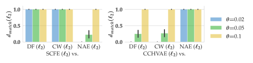
Figure 5: Analyzing to what extent different counterfactual explanation methods and adversarial example generation methods are empirically equivalent for the logistic regression classifier with German Credit data. We compute $d_{\text{match}}$ from (12) with varying thresholds $\theta=\{0.02,0.05,0.1\}$. Missing bars indicate that there was no match.

We also include results for Neural Networks in Appendix D.2.

D.2 Empirical Evaluation with ANN

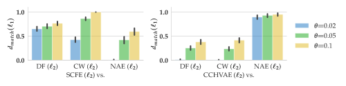
(a) Adult

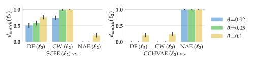
(b) COMPAS

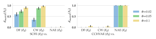
(c) German Credit

Figure 6: Analyzing to what extent different counterfactual explanations and adversarial examples are empirically equivalent for the 2-layer ANN classifier. To do that, we compute $d_{match}$ from (12) with varying thresholds $\theta=\{0.02,0.05,0.1\}$. Missing bars indicate that there was no match.

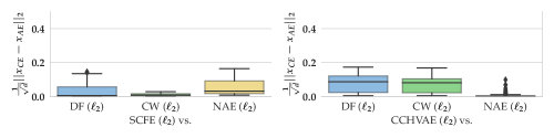
(a) Adult

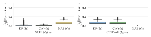
(b) COMPAS

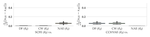
(c) German Credit

Figure 7: Distribution of instance wise norm comparisons for the logistic regression model. We show the distribution of cost comparisons across negatively predicted instances ($\hat{y}=0$) for which we computed adversarial examples and counterfactual explanations.

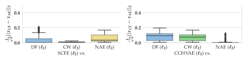
(a) Adult

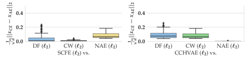
(b) COMPAS

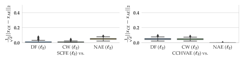
(c) German Credit

Figure 8: Distribution of instance wise norm comparisons for the 2-layer ANN. We show the distribution of cost comparisons across negatively predicted instances ($\hat{y}=0$) for which we computed adversarial examples and counterfactual explanations.

References

- Akhtar and Mian [2018] Naveed Akhtar and Ajmal Mian. Threat of adversarial attacks on deep learning in computer vision: A survey. Ieee Access, 6:14410–14430, 2018.
- Arjovsky et al. [2017] Martin Arjovsky, Soumith Chintala, and Léon Bottou. Wasserstein gan. arxiv 2017. arXiv preprint arXiv:1701.07875, 30, 2017.
- Ballet et al. [2019] Vincent Ballet, Xavier Renard, Jonathan Aigrain, Thibault Laugel, Pascal Frossard, and Marcin Detyniecki. Imperceptible adversarial attacks on tabular data. arXiv preprint arXiv:1911.03274, 2019.
- Barocas et al. [2020] Solon Barocas, Andrew D Selbst, and Manish Raghavan. The hidden assumptions behind counterfactual explanations and principal reasons. In Proceedings of the 2020 Conference on Fairness, Accountability, and Transparency, pages 80–89, 2020.
- Biggio et al. [2012] Battista Biggio, Blaine Nelson, and Pavel Laskov. Poisoning attacks against support vector machines. In ICML, 2012.
- Bora et al. [2017] Ashish Bora, Ajil Jalal, Eric Price, and Alexandros G Dimakis. Compressed sensing using generative models. In International Conference on Machine Learning, pages 537–546. PMLR, 2017.
- Browne and Swift [2020] Kieran Browne and Ben Swift. Semantics and explanation: why counterfactual explanations produce adversarial examples in deep neural networks. arXiv preprint arXiv:2012.10076, 2020.
- Carlini and Wagner [2017] Nicholas Carlini and David Wagner. Towards evaluating the robustness of neural networks. In 2017 ieee symposium on security and privacy (sp), pages 39–57. IEEE, 2017.
- Cartella et al. [2021] Francesco Cartella, Orlando Anunciacao, Yuki Funabiki, Daisuke Yamaguchi, Toru Akishita, and Olivier Elshocht. Adversarial attacks for tabular data: Application to fraud detection and imbalanced data. arXiv preprint arXiv:2101.08030, 2021.
- Cisse et al. [2017] Moustapha Cisse, Yossi Adi, Natalia Neverova, and Joseph Keshet. Houdini: Fooling deep structured prediction models. arXiv preprint arXiv:1707.05373, 2017.
- Dua and Graff [2017] Dheeru Dua and Casey Graff. UCI machine learning repository, 2017. URL http://archive.ics.uci.edu/ml.
- Freiesleben [2020] Timo Freiesleben. Counterfactual explanations & adversarial examples–common grounds, essential differences, and potential transfers. arXiv preprint arXiv:2009.05487, 2020.
- Garreau and Luxburg [2020] Damien Garreau and Ulrike Luxburg. Explaining the explainer: A first theoretical analysis of lime. In International Conference on Artificial Intelligence and Statistics (AISTATS), pages 1287–1296. PMLR, 2020.
- Goodfellow et al. [2014] Ian J Goodfellow, Jonathon Shlens, and Christian Szegedy. Explaining and harnessing adversarial examples. arXiv preprint arXiv:1412.6572, 2014.
- Gouk et al. [2021] Henry Gouk, Eibe Frank, Bernhard Pfahringer, and Michael J Cree. Regularisation of neural networks by enforcing lipschitz continuity. Springer, 2021.
- Hardt and Ma [2017] Moritz Hardt and Tengyu Ma. Identity matters in deep learning. In International Conference on Learning Representations (ICLR), 2017.
- Joshi et al. [2019] Shalmali Joshi, Oluwasanmi Koyejo, Warut Vijitbenjaronk, Been Kim, and Joydeep Ghosh. Towards realistic individual recourse and actionable explanations in black-box decision making systems. arXiv preprint arXiv:1907.09615, 2019.
- Karimi et al. [2020a] Amir-Hossein Karimi, Gilles Barthe, Borja Balle, and Isabel Valera. Model-agnostic counterfactual explanations for consequential decisions. In International Conference on Artificial Intelligence and Statistics (AISTATS), pages 895–905. PMLR, 2020a.
- Karimi et al. [2020b] Amir-Hossein Karimi, Gilles Barthe, Bernhard Schölkopf, and Isabel Valera. A survey of algorithmic recourse: definitions, formulations, solutions, and prospects. arXiv preprint arXiv:2010.04050, 2020b.
- Karimi et al. [2020c] Amir-Hossein Karimi, Julius von Kügelgen, Bernhard Schölkopf, and Isabel Valera. Algorithmic recourse under imperfect causal knowledge: a probabilistic approach. arXiv preprint arXiv:2006.06831, 2020c.
- Karimi et al. [2021] Amir-Hossein Karimi, Bernhard Schölkopf, and Isabel Valera. Algorithmic recourse: from counterfactual explanations to interventions. In Proceedings of the 2021 ACM Conference on Fairness, Accountability, and Transparency (FAccT), pages 353–362, 2021.
- Kingma and Ba [2014] Diederik P Kingma and Jimmy Ba. Adam: A method for stochastic optimization. arXiv preprint arXiv:1412.6980, 2014.
- Kurakin et al. [2016] Alexey Kurakin, Ian Goodfellow, Samy Bengio, et al. Adversarial examples in the physical world, 2016.
- Lundberg and Lee [2017] Scott Lundberg and Su-In Lee. A unified approach to interpreting model predictions. arXiv preprint arXiv:1705.07874, 2017.
- Mattu et al. [2016] S Mattu, L Kirchner, and J Angwin. How we analyzed the compas recidivism algorithm. ProPublica, 2016.
- Moosavi-Dezfooli et al. [2016] Seyed-Mohsen Moosavi-Dezfooli, Alhussein Fawzi, and Pascal Frossard. Deepfool: a simple and accurate method to fool deep neural networks. In Proceedings of the IEEE conference on computer vision and pattern recognition, pages 2574–2582, 2016.
- Pawelczyk et al. [2020] Martin Pawelczyk, Klaus Broelemann, and Gjergji Kasneci. Learning model-agnostic counterfactual explanations for tabular data. In Proceedings of The Web Conference 2020, pages 3126–3132, 2020.
- Rawal and Lakkaraju [2020] Kaivalya Rawal and Himabindu Lakkaraju. Interpretable and interactive summaries ofactionable recourses. arXiv preprint arXiv:2009.07165, 2020.
- Ribeiro et al. [2016] Marco Tulio Ribeiro, Sameer Singh, and Carlos Guestrin. " why should i trust you?" explaining the predictions of any classifier. In Proceedings of the 22nd ACM SIGKDD international conference on knowledge discovery and data mining, pages 1135–1144, 2016.
- Rosenfeld et al. [2020] Elan Rosenfeld, Ezra Winston, Pradeep Ravikumar, and Zico Kolter. Certified robustness to label-flipping attacks via randomized smoothing. In International Conference on Machine Learning, pages 8230–8241. PMLR, 2020.
- Shafahi et al. [2018] Ali Shafahi, W Ronny Huang, Mahyar Najibi, Octavian Suciu, Christoph Studer, Tudor Dumitras, and Tom Goldstein. Poison frogs! targeted clean-label poisoning attacks on neural networks. In NeurIPS, 2018.
- Simonyan et al. [2013] Karen Simonyan, Andrea Vedaldi, and Andrew Zisserman. Deep inside convolutional networks: Visualising image classification models and saliency maps. arXiv preprint arXiv:1312.6034, 2013.
- Sundararajan et al. [2017] Mukund Sundararajan, Ankur Taly, and Qiqi Yan. Axiomatic attribution for deep networks. In International Conference on Machine Learning (ICML), pages 3319–3328. PMLR, 2017.
- Szegedy et al. [2013] Christian Szegedy, Wojciech Zaremba, Ilya Sutskever, Joan Bruna, Dumitru Erhan, Ian Goodfellow, and Rob Fergus. Intriguing properties of neural networks. arXiv preprint arXiv:1312.6199, 2013.
- Tavallali et al. [2021] Pooya Tavallali, Vahid Behzadan, Peyman Tavallali, and Mukesh Singhal. Adversarial poisoning attacks and defense for general multi-class models based on synthetic reduced nearest neighbors. arXiv, 2021.
- Ustun et al. [2019] Berk Ustun, Alexander Spangher, and Yang Liu. Actionable recourse in linear classification. Proceedings of the Conference on Fairness, Accountability, and Transparency, Jan 2019. doi: 10.1145/3287560.3287566. URL http://dx.doi.org/10.1145/3287560.3287566.
- Van Looveren and Klaise [2019] Arnaud Van Looveren and Janis Klaise. Interpretable counterfactual explanations guided by prototypes. arXiv preprint arXiv:1907.02584, 2019.
- Venkatasubramanian and Alfano [2020] Suresh Venkatasubramanian and Mark Alfano. The philosophical basis of algorithmic recourse. In Proceedings of the 2020 Conference on Fairness, Accountability, and Transparency (FAT*), pages 284–293, 2020.
- Verma et al. [2020] Sahil Verma, John Dickerson, and Keegan Hines. Counterfactual explanations for machine learning: A review. arXiv preprint arXiv:2010.10596, 2020.
- Wachter et al. [2017] Sandra Wachter, Brent Mittelstadt, and Chris Russell. Counterfactual explanations without opening the black box: Automated decisions and the gdpr. In Harvard Journal & Technology, 2017.
- Zhao et al. [2018] Zhengli Zhao, Dheeru Dua, and Sameer Singh. Generating natural adversarial examples. In International Conference on Learning Representations (ICLR), 2018.