A Squeezed Vacuum State Laser with Zero Diffusion

Abstract

We propose a method for building a squeezed vacuum state laser with zero diffusion, which results from the introduction of the reservoir engineering technique into the laser theory. As well as the reservoir engineering, our squeezed vacuum laser demands the construction of an effective atom-field interaction. And by building an isomorphism between the cavity field operators in the effective and the Jaynes-Cummings Hamiltonians, we derive the equations of our effective laser directly from the conventional laser theory. Our method, which is less susceptible to errors than reservoir engineering, can be extended for the construction of other nonclassical state lasers, and our squeezed vacuum laser can contribute to the newly emerging field of gravitational interferometry.

I Introduction

The laser theory is one of the central developments in the physics of radiation-matter interaction. Based on the theoretical framework provided by Townes and Schawlow [1], the first laser, built by Maiman [2], date back to the 1960s, and has since played a major role both in basic and applied physics, with applications in many technical aspects of modern society. The quantum theory of the laser was built basically from contributions led by H. Haken [3], W. E. Lamb [4], and M. Lax [5], from which are derived the more realistic models where a transmitting window [6], and the pumping statistics of the lasing atoms [7] are included.

Among many others, we mention the uses of lasers for cooling and trapping atoms [8], for Bose-Einstein condensation in dilute gases of alkali atoms [9], for the development of optical tweezers and their application in biological and physical sciences [10], and for generating ultrashort high-intensity laser pulses extensively used across physics and chemistry [11]. These achievements draw a broader picture of the unique progress that quantum optics has undergone since the 1980s. In addition to this picture we mention the generations of squeezed states of the radiation field [12], essential for enhancing interferometric sensitivity [13], and today a critical challenge for the development of gravitational wave interferometry [14, 15, 16]. We also mention the applications of squeezed states in optical waveguide tap [17], quantum nondemolition measurements [15], quantum information processing [18], and quantum metrology [19]. There is also the development of different sources for generating entangled photon states, used for investigating fundamentals of quantum mechanics [20].

Parallel to the developments of quantum optics, we witnessed the emergence of quantum communication and computation, which resulted in the new and promising field of quantum information theory [21]. The need for implementation of quantum logic operations demanded new techniques for engineering nonclassical states [22], effective interactions [23, 24] and reservoirs [25, 26] for phase coherence control. These demands have pushed the physics of the radiation-matter interaction to a new level through platforms such as cavity quantum electrodynamics [27], trapped ions [28], circuit quantum electrodynamics [29], and all related topics. Regarding coherence control, a key issue for the construction of a squeezed vacuum laser with zero diffusion, many methods have been designed [30]; however, the reservoir engineering [25] —which seems inspired by the laser theory— is of particular interest here. Its basic idea is to submit the system of interest, say a dissipative cavity mode (described by the creation and annihilation operators $a^{{\dagger}}$ and $a$, and whose particular state $\left|\Psi\right\rangle$ we intend to protect from the action of the environment), to an interaction with an auxiliary strongly dissipative system as, for example, a two-level atom (described by the Pauli raising and lowering operators $\sigma_{+}$ and $\sigma_{-}$). This interaction must then be engineered so that it takes the bilinear form

$$\chi\left(AS_{+}+A^{{\dagger}}S_{-}\right),$$ (1)

with $\chi$ being an effective atom-field coupling and $A^{{\dagger}},A$ ($S_{+},S_{-}$) defined by a canonical transformation on the original operators for the cavity mode: $a^{{\dagger}},a$ (auxiliary atom: $\sigma_{+},\sigma_{-}$ ), with the central requirement $A\left|\Psi\right\rangle=0$. The master equation for the cavity mode, coming from reservoir engineering, is given by

$$\dot{\rho}=\left(\Gamma/2\right)\left(2A\rho A^{{\dagger}}-A^{{\dagger}}A\rho-\rho A^{{\dagger}}A\right)$$

$$+\left(\tilde{\Gamma}/2\right)\left(2a\rho a^{{\dagger}}-a^{{\dagger}}a\rho-\rho a^{{\dagger}}a\right),$$ (2)

with the assumption $\Gamma\propto\chi\gg\tilde{\Gamma}$. It is therefore clear that the Lindbladian for $a^{{\dagger}},a$ acts as a perturbation over that for $A^{{\dagger}},A$, causing the fidelity of the protected state, necessarily an eigenstate of $A$ with null eigenvalue [25] ($A\left|\Psi\right\rangle=0$), to be slightly less than unity, since $\mathcal{F}\propto 1-\tilde{\Gamma}/\Gamma$.

Compared to the method of state protection through engineered reservoir, the conventional laser mechanism is far more generous since the stringent requirement $A\left|\Psi\right\rangle=0$ is relaxed, with the laser coherent steady state $\left|\alpha\right\rangle$ being an eigenstate of $a$ with non null eigenvalue, $a\left|\alpha\right\rangle=\alpha\left|\alpha\right\rangle$. Nonetheless, this relaxed condition implies the coherence loss of the laser stationary state due to phase diffusion. Our squeezed vacuum laser, however, despite based on the requirement $A\left|\Psi\right\rangle=0$, is also more generous than the engineered reservoir method, since the Lindbladian for $a^{{\dagger}},a$ —which acts in the engineered reservoirs to prevent the fidelity from being equal to the unit— is absent from the laser master equation. We must return to this interesting point later.

Our strategy here is to bring the reservoir engineering method into the laser mechanism, aiming to produce a steady squeezed vacuum state preserving phase coherence. From the reservoir engineering we must implement the bilinear interaction of the cavity mode with the auxiliary system, now the laser active medium. By its turn, from the laser theory we subject the active medium to a linear amplification process which, due to its interaction with the cavity mode, feeds it by stimulated emission concomitantly producing a saturation which helps constructing the far-from-equilibrium steady state. Then, by adding together the reservoir engineering technique to the laser theory, we should be able to build a laser with zero diffusion or zero line width, and therefore a decoherence-free state of the cavity field.

As it should be clear in the next section, the effective bilinear Hamiltonian required for building up the squeezed vacuum laser is a particular form of that in Eq. (1), given by

$$\chi\left(A\sigma_{+}+A^{{\dagger}}\sigma_{-}\right),$$ (3)

which suggests an isomorphism between this interaction and the Jaynes-Cummings model, a map between the field operators $a\leftrightarrow A$ and $a^{{\dagger}}\leftrightarrow A^{{\dagger}}$. This isomorphism would allow us to derive the equations of our effective laser directly from those of the conventional laser theory. For the construction of such an isomorphism relation we must derive a vector basis for the cavity field, $\left\{\left|n\right\rangle_{A}\right\}$, on which the action of our generalized operators $\left(A^{{\dagger}},A\right)$ emulate that of the usual creation and annihilation operators $\left(a^{{\dagger}},a\right)$ in the Fock space $\left\{\left|n\right\rangle\right\}$. With this, we immediately derive the generalized master equation that describes, in the above-threshold regime, the construction of the steady squeezed vacuum state. In short, all we have to do is to establish the isomorphism between the cavity field operators in our squeezed vacuum laser and in the conventional coherent state laser; given the isomorphism, the equations for our laser are automatically settled.

We stress here that the constructed isomorphism between the field operators in the effective and the Jaynes-Cummings Hamiltonians automatically results in the engineered Lindbladian $\left(\Gamma/2\right)\left(2A\rho A^{{\dagger}}-A^{{\dagger}}A\rho-\rho A^{{\dagger}}A\right)$, differently from what happens in the original reservoir engineering protocol [25], in which a set of approximations is required to obtain the desired Lindbladian. In other words, the engineered Lindbladian comes as a gift from the constructed isomorphism, avoiding the set of approximation imposed by the original reservoir engineering method. Furthermore, in the derivation of the engineered Lindbladian through the constructed isomorphism, we have the advantage of eliminating the unwanted Lindbladian for $a^{{\dagger}},a$ which, as observed above, acts as a perturbation over that for $A^{{\dagger}},A$ (causing the fidelity of a protected state to be slightly less than unity). Although the method we have used is not exactly that of reservoir engineering as presented in [25], all the main ingredientes of the latter method are actually present in our conctruction: the engineering of the effective atom-field interation and, consequently, of the associated Lindbladian.

A laser with zero linewidth is most useful for a variety of application, among which we mention optical sensing, metrology, higher order coherent communication, high-precision detection, and laser spectroscopy [31]. Therefore, the method here presented can contribute to or inspire the design of lasers with exceedingly small diffusion and linewidth, with broad technological applications.

Squeezed states are most efficiently generated from optical parametric down-conversion in a non-linear $\chi^{\left(2\right)}$ crystal [32, 33]. We also mention the generation of squeezed states by four wave mixing in an optical cavity [34, 33]. However, our purpose here is to demonstrate the possibility of generating squeezed state of light through the laser mechanism, with the required nonlinearity being constructed through the atom-field interaction itself. The squeezing of cavity-field states through their effective interaction with atoms have been systematically pursued in cavity quantum electrodynamics [35].

Our paper is organized as follows: In Section II we present a scheme, based on the adiabatic elimination of fast variables, for the construction of the effective Hamiltonian required for the operation of the squeezed vacuum laser. In Section III we construct the isomorphism between the cavity field operators in the effective and the Jaynes-Cummings interactions, and in Section IV we present the master equation for the squeezed vacuum laser and the numerical analysis demonstrating the effectiveness of our method. Finally, in Section V we present our conclusions.

II The effective atom-field interaction

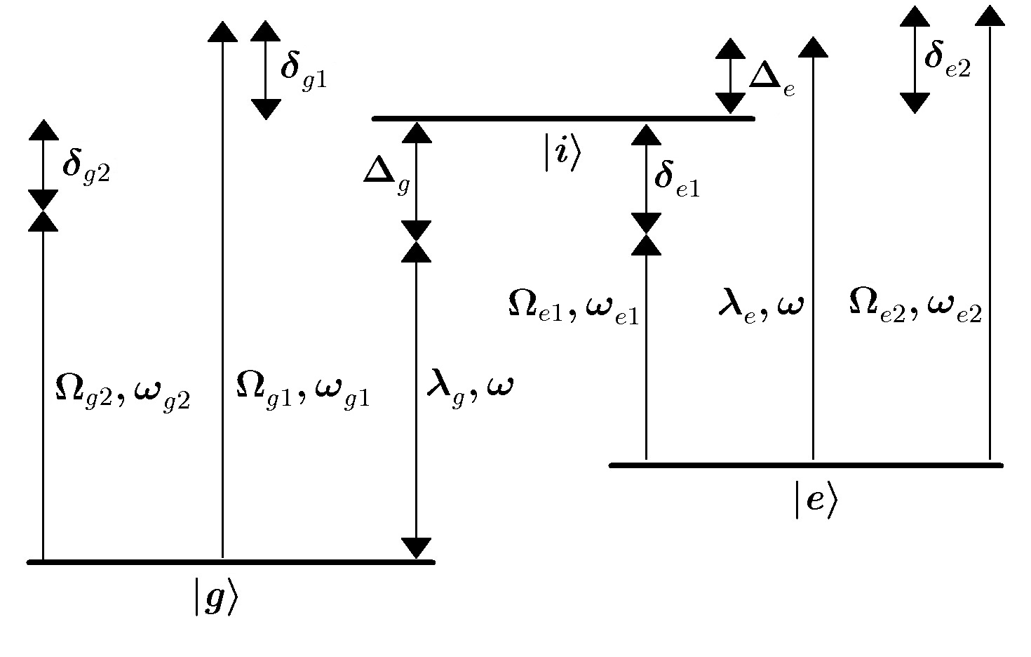
Figure 1: Sketch of the $\mathbb{\varLambda}$ configuration to engineer the effective interaction for building up the squeezed vacuum laser. The cavity mode ($\omega$) is used to promote the Raman-type transitions $g$ $\leftrightarrow$ $i$ and $e$ $\leftrightarrow$  $i$, with detunings $\Delta_{g}=\omega_{i}-\omega$ and $\Delta_{e}=\omega_{0}+\omega-\omega_{i}$, and coupling strengths $\lambda_{g}$ and $\lambda_{e}$. Two pairs of laser beams ($\omega_{g\ell}$ and $\omega_{e\ell}$, $\ell=1,2$) with detunings $\delta_{g1}=\omega_{g1}-\omega_{i}$, $\delta_{g2}=\omega_{i}-\omega_{g2}$, $\delta_{e1}=\omega_{i}-\omega_{0}-\omega_{e1}$ and $\delta_{e2}=\omega_{0}+\omega_{e2}-\omega_{i}$ and coupling strengths $\Omega_{g\ell}$ and $\Omega_{e\ell}$

The first step for achieving our goal is to engineer the atom-field interaction through which we implement the amplification-saturation mechanism building up and sustaining our squeezed vacuum state. The effective interaction follows from considering the transitions induced by quantum and classical fields in a three-level Lambda-type configuration, as depicted in Fig. 1. The intermediate (more-excited) atomic level $\left|i\right\rangle$ must be considered, apart from the lasing levels $\left|g\right\rangle$ and $\left|e\right\rangle$. The cavity mode ($\omega$) is used to promote the Raman-type transitions $g$ $\longleftrightarrow$ $i$ and $e\longleftrightarrow i$, with detunings $\Delta_{g}=\omega_{i}-\omega$ and $\Delta_{e}=\omega_{0}+\omega-\omega_{i}$, and coupling strengths $\lambda_{g}$ and $\lambda_{e}$. Two pairs of laser beams ($\omega_{g\ell}$ and $\omega_{e\ell}$, $\ell=1,2$) help to excite the same atomic transitions with detunings $\delta_{g1}=\omega_{g1}-\omega_{i}$, $\delta_{g2}=\omega_{i}-\omega_{g2}$, $\delta_{e1}=\omega_{i}-\omega_{0}-\omega_{e1}$ and $\delta_{e2}=\omega_{0}+\omega_{e2}-\omega_{i}$ and coupling strengths $\Omega_{g\ell}$ and $\Omega_{e\ell}$. The Hamiltonian describing the process is given by $H(t)=H_{0}+V(t)$, where

$$H_{0}= \omega a^{{\dagger}}a+\omega_{0}\sigma_{ee}+\omega_{i}\sigma_{ii}\text{,}$$ (4a)

$$V(t)= \lambda_{g}a\sigma_{ig}+\lambda_{e}a\sigma_{ie}+$$

$${\textstyle\sum\nolimits_{\ell}}\left(e^{-i\omega_{g\ell}t}\Omega_{g\ell}\sigma_{ig}+e^{-i\omega_{e\ell}t}\Omega_{e\ell}\sigma_{ie}\right)+h.c.\text{,}$$ (4b)

using the Pauli operators $$\sigma_{rs}=\left|r\right\rangle\left\langle s\right| r,s \lambda_{g} = \lambda_{e}=\lambda \Omega_{g1}= \Omega_{g2}=- \Omega_{e1}=- \Omega_{e2} \delta_{g1}=\delta_{g2}=\delta_{e1}/\kappa=\delta_{e2}/\kappa \Delta_{g}=\delta_{e1} \Delta_{e}=\delta_{g1} \delta_{r\ell}\gg\Omega_{r\ell}\gg\bar{n}\lambda \bar{n} \mathcal{H}(t)$$, with denoting the atomic levels. In what follows we assume , , , and . Then, under the set of parameter , with being the average photon number in the cavity, we verify that, in the interaction picture, the non-diagonal Hamiltonian consists of highly oscillatory terms such that, to a good approximation, we obtain the second-order effective Hamiltonian [36]

$$H_{eff}=-i\mathcal{H}(t)\int_{0}^{t}d\tau\mathcal{H}(\tau)=g\left(A\sigma_{+}+A^{{\dagger}}\sigma_{-}\right)\text{,}$$ (5)

where $\sigma_{+}=|e\rangle\langle g|$, $\sigma_{-}=|g\rangle\langle e|$ and the coupling strength is given by $g=\sqrt{1-\kappa^{2}}\lambda\Omega_{g1}/\delta_{e1}$, with $\kappa=\delta_{e1}/\delta_{g1}$, and the generalized operators read

$$A=\frac{a+\kappa a^{{\dagger}}}{\sqrt{1-\kappa^{2}}}\text{, \ \ }A^{{\dagger}}=\frac{a^{{\dagger}}+\kappa a}{\sqrt{1-\kappa^{2}}}\text{,}$$ (6)

with $\left[A,A^{{\dagger}}\right]=\left[a,a^{{\dagger}}\right]=1$.

In order to verify the validity of the approximations leading from $V(t)$ to $H_{eff}$, we plot in Figs. 2(a) and (b) the variances of the quadratures $X_{1}=\left(a^{\dagger}+a\right)/2$ and $X_{2}=\left(a-a^{\dagger}\right)/2i$ for the field states generated by both the full and the effective Hamiltonians in Eqs. (4) and (5), against $gt$, i.e. the number of cycles of the effective coupling. We start with the atom in the excited state $\left|e\right\rangle$ and the cavity mode in the vacuum state $\left|0\right\rangle$, considering, in units of the Rabi frequency $\lambda$, the parameters $\delta_{g1}=10^{3}$, $\delta_{e1}=6\times 10^{2}$, $\Omega_{g1}=40$, and $g=0.05$, such that $\kappa=0.6$. In Figs. 2(a) and (b) the straight and dotted lines refer to the effective and full Hamiltonians, respectively, showing a good agreement between both curves up to $gt\approx 7$. We have also plotted in Figs. 2(c) and (d) the excitations $\left\langle a^{\dagger}a\right\rangle(t)$ and $\left\langle\sigma_{ee}\right\rangle(t)$ against $gt$, and we again see a very good agreement between the curves generated by the full and the effective Hamiltonians until the same $gt\approx 7$.

Regarding the engineering of the effective atom-field interaction (5), a detailed account on Raman transition in cavity quantum electrodynamics can be found in Ref. [38]. We note that the atomic level configuration we have used to engineer the required interaction is certainly not unique; it can be engineered from other level configuration using more or less classical fields. Finally, we stress that in engineering the effective Hamiltonian (5) we have not take into account the usually small amplitude and phase fluctuations of the required laser beams, which would indeed result in some phase diffusion of our squeezed vacuum laser. At this point we mention that another proposal to achieve squeezed lasing has been presented in which the cavity is parametric driven with the help of a non-linear $\chi^{\left(2\right)}$ crystal inside the cavity [39]. Our engineered atom-field interaction thus repalces the parametric driven process in Ref. [39], dispensing the non-linear crystal inside the cavity and the coherent drive of the cavity mode. However, since our laser requires the effective atom-field interaction, it present an operating timescale after which it must be restarted.

III The isomorphism between the $A^{{\dagger}},A$ and $a^{\dagger},a$ algebras

Having engineered the required interaction (5), we now start to construct the vector basis $\left\{\left|n\right\rangle_{A}\right\}$ for the cavity field, in whose states $\left|n\right\rangle_{A}$ the action of operators $A^{{\dagger}}A$, $A^{{\dagger}}$ and $A$, must lead to the same relations as those resulting from the actions of $a^{{\dagger}}a,$ $a^{{\dagger}}$ and $a$ on the Fock basis $\left\{\left|n\right\rangle\right\}$, i.e.:

$$A^{{\dagger}}A\left|n\right\rangle_{A} =n\left|n\right\rangle_{A},$$ (7a)

$$A^{{\dagger}}\left|n\right\rangle_{A} =\sqrt{n+1}\left|n+1\right\rangle_{A},$$ (7b)

$$A\left|n\right\rangle_{A} =\sqrt{n}\left|n-1\right\rangle_{A}.$$ (7c)

All the basis states $$\left\{\left|n\right\rangle_{A}\right\} \left|0\right\rangle_{A}$$ are constructed from the vacuum state , starting from the relation

$$A\left|0\right\rangle_{A}=0\text{,}$$ (8)

which enables us to determine the probability amplitudes $c_{n}$ defining the superposition $\left|0\right\rangle_{A}=\sum\nolimits_{n}c_{n}\left|n\right\rangle$. Considering the operator $A$ as given by Eq. (6), we first compute the vacuum state from Eq. (8) and then, using the relation $\left(A^{{\dagger}}\right)^{n}\left|0\right\rangle_{A}/\sqrt{n!}$, we derive all the even and odd generalized excitations, given by

$$\left|2m\right\rangle_{A}=\frac{\left(1-\kappa^{2}\right)^{1/4}}{\sqrt{\left(2m\right)!}}\sum\limits_{n=0}^{\infty}\left(-\kappa\right)^{n-m}\sqrt{\frac{\left(2n-1\right)!!}{\left(2n\right)!!}}$$

$$\times\sum\limits_{\ell=0}^{m}\binom{m}{\ell}\left(-\kappa^{2}\right)^{\ell}\frac{\left(2n\right)!!}{\left[2\left(n+\ell-m\right)\right]!!}\frac{\left[2\left(n+\ell\right)-1\right]!!}{\left(2n-1\right)!!}\left|2n\right\rangle\text{,}$$ (9a)

$$\left|2m+1\right\rangle_{A}=\frac{\left(1-\kappa^{2}\right)^{3/4}}{\sqrt{\left(2m+1\right)!}}\sum\limits_{n=0}^{\infty}\left(-\kappa\right)^{n-m}\sqrt{\frac{\left(2n+1\right)!!}{\left(2n\right)!!}}$$

$$\times\sum\limits_{\ell=0}^{m}\binom{m}{\ell}\left(-\kappa^{2}\right)^{\ell}\frac{\left(2n\right)!!}{\left[2\left(n+\ell-m\right)\right]!!}\frac{\left[2\left(n+\ell\right)+1\right]!!}{\left(2n+1\right)!!}\left|2n+1\right\rangle\text{.}$$ (9b)

The basis defined by the even and odd number states given by Eqs. (9), together with the laser model establishes the isomorphism between the laser field generated by the interaction from Eq. 3, written in the new basis, and the usual laser field, in the Fock basis, since their master equations are similar, containing each the Liouville-Von Neumman term and the cavity dissipative term in the Lindblad form, referring to the loss of an Harmonic Oscillator (HO) to the enviroment. The Liouville-Von Neumman term would be equal in both lasers, once we use the Hamiltonian in the new basis, as in Eq. 3, and since now we have a system guided by an interaction in the form of Jaynes-Cummings, as describing an HO, naturally we can say that the cavity dissipates in the Lindblad form. Knowing that the steady state of the conventional laser is the coherent state $\left|\alpha\right\rangle$ (owing to the Jaynes-Cummings atom-field interaction), it is then automatic to derive the steady state of our laser, which results from the effective Hamiltonian (5). Once the isomorphism is established, all we have to do is to describe the coherent state in the vector basis $\left\{\left|n\right\rangle_{A}\right\}$, i.e., $\left|\alpha\right\rangle_{A}=D_{A}(\alpha)\left|0\right\rangle_{A}=\exp\left(\alpha A^{{\dagger}}-\alpha^{\ast}A\right)\left|0\right\rangle_{A}=e^{-\left|\beta\right|^{2}/2}e^{\beta a^{{\dagger}}}e^{-\beta^{\ast}a}\left|0\right\rangle_{A}$, with $\beta=\left(\alpha-\kappa\alpha^{\ast}\right)/\sqrt{1-\kappa^{2}}$. We obtain, expanded in the usual Fock basis $\left\{\left|n\right\rangle\right\}$, the state

$$\left|\alpha\right\rangle_{A}=(1-\kappa^{2})^{1/4}e^{\left(\kappa\alpha^{2}-\left|\alpha\right|^{2}\right)/2}$$ (10)

$$\sum\limits_{n=0}^{\infty}\sqrt{n!}\left(\sum\limits_{\ell=0}^{n}\left(\frac{\kappa}{2}\right)^{\ell/2}\frac{\beta^{n-\ell}}{\left(n-\ell\right)!\ell!}H_{\ell}\left(x\right)\right)\left|n\right\rangle,$$ (11)

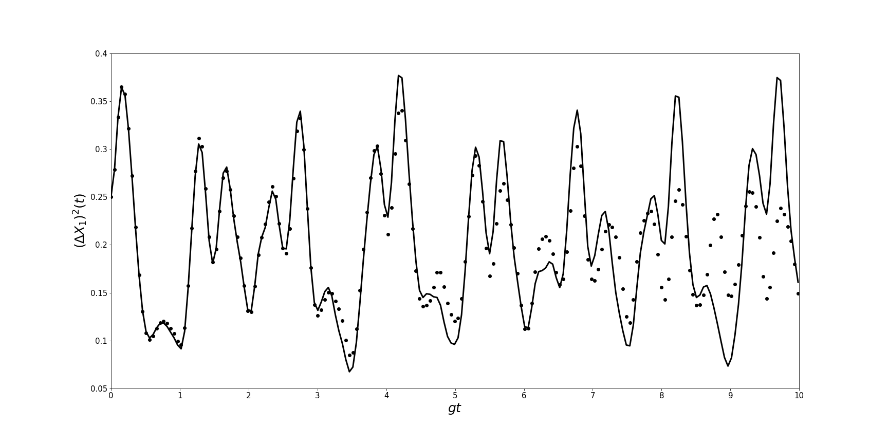
(a)

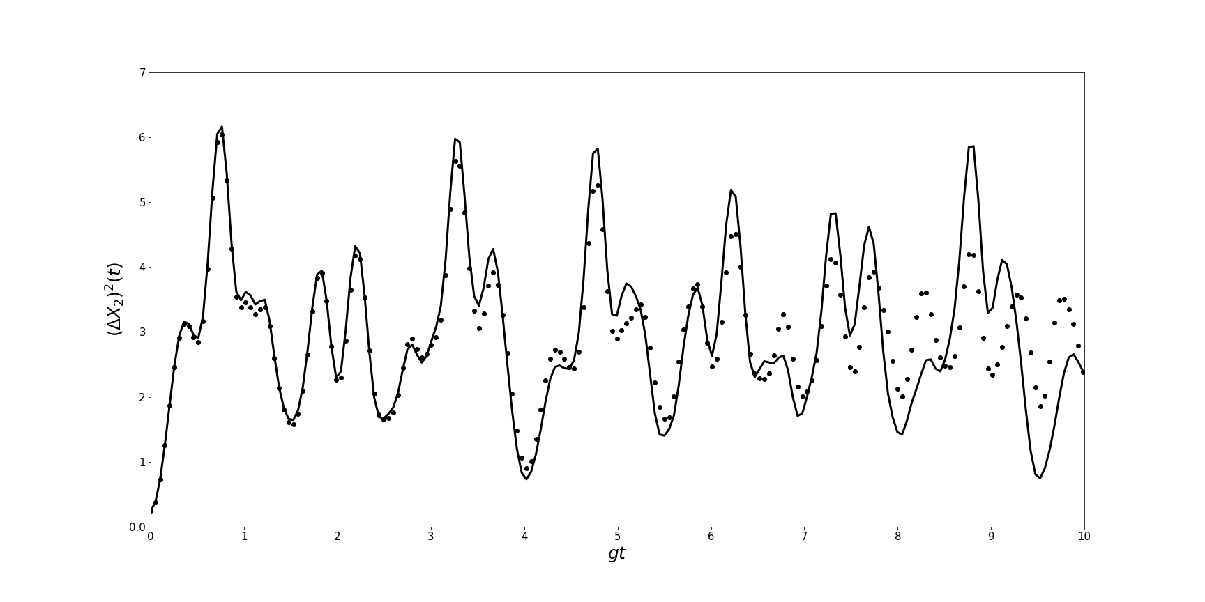
(b)

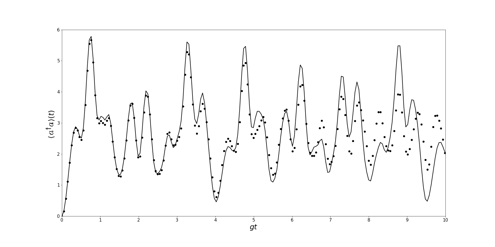
(c)

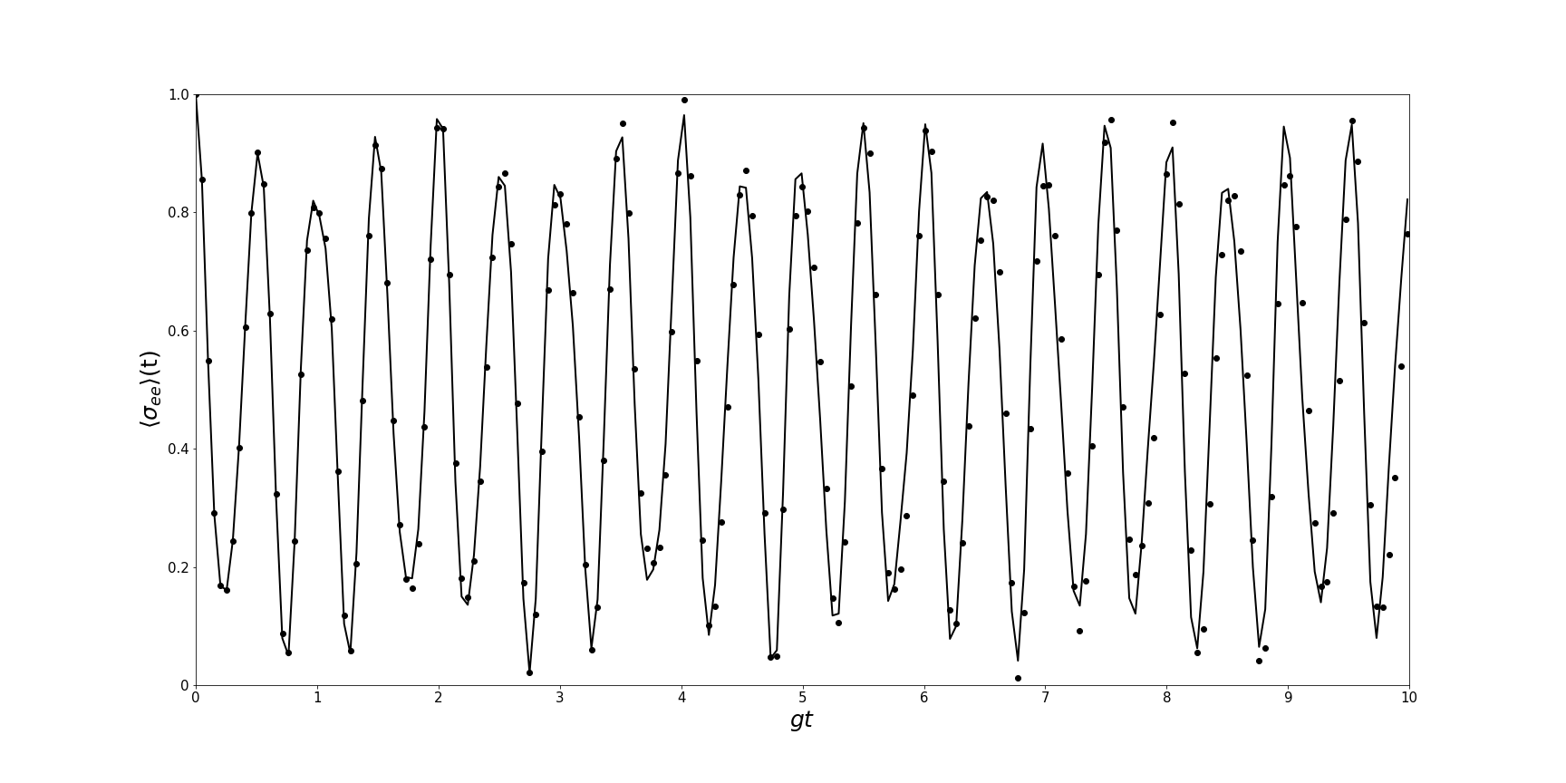
(d)

Figure 2: Validity of the Effective interaction. The the variances (a), $\left(\Delta X_{1}\right)^{2}(t)$ and (b), $\left(\Delta X_{2}\right)^{2}(t)$, and the excitations (c), $\left\langle a^{\dagger}a\right\rangle(t)$ and (d), $\left\langle\sigma_{ee}\right\rangle(t)$ in function of $gt$, for the field states generated by the effective and full Hamiltonians (straight and dotted lines, respectively). We have started with the atom and the cavity mode in the excited and the vacuum state, $\left|e\right\rangle\left|0\right\rangle$, considering, in units of the Rabi frequency $\lambda$, the parameters $\delta_{g1}=10^{3}$, $\delta_{e1}=6\times 10^{2}$, $\Omega_{g1}=40$, and $g=0.05$, such that $\kappa=0.6$.

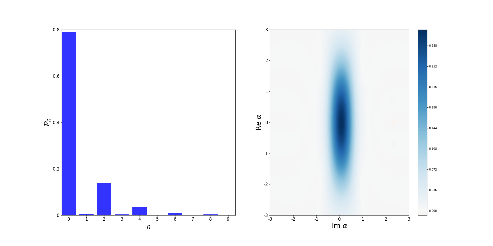
(a)

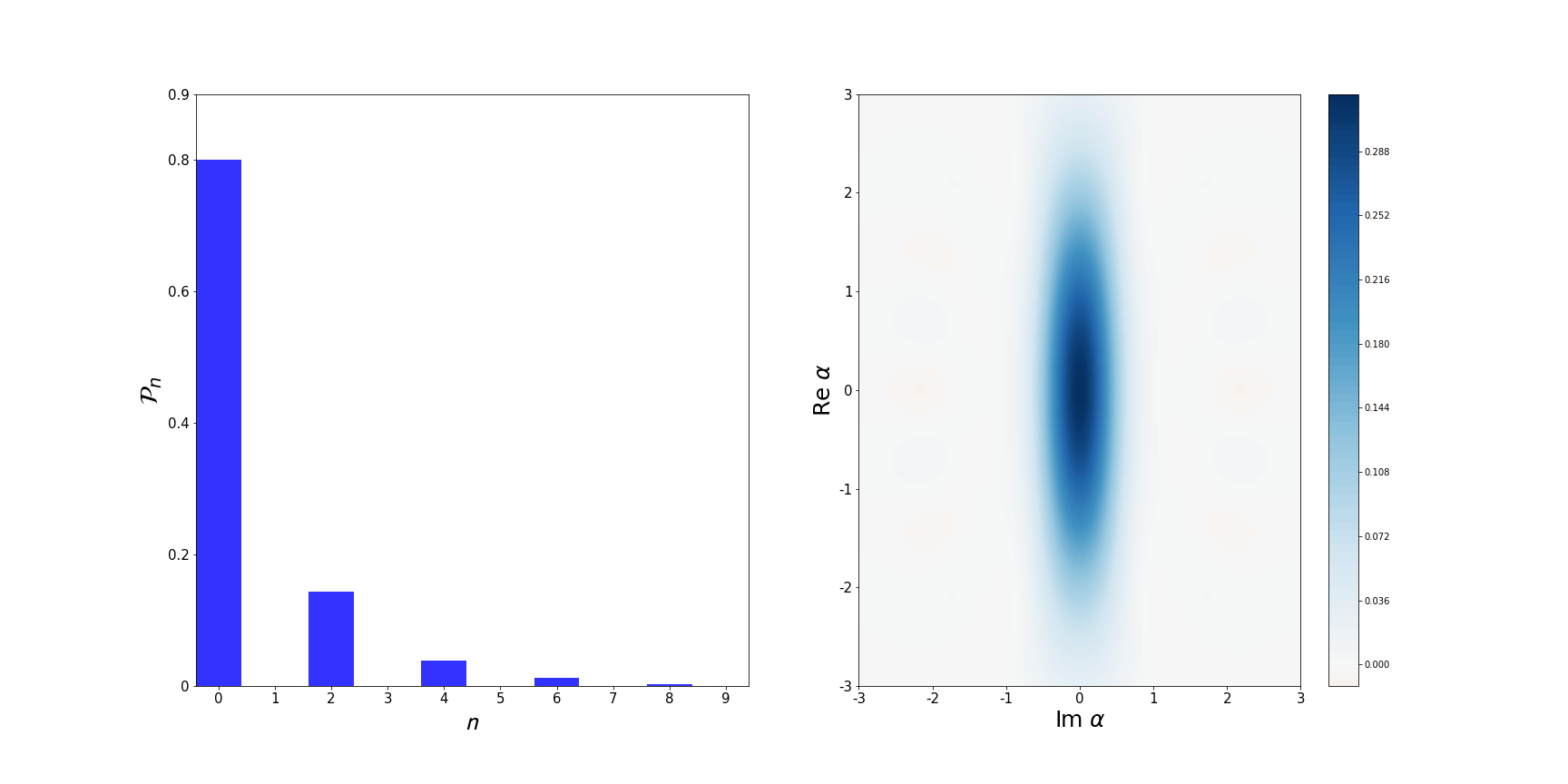
(b)

Figure 3: The photon number distribution $\mathcal{P}_{n}$ and the Wigner function.(a), generated by the effective Hamiltonian for $\alpha=0.18$ and $r=0.69$.(b), ideal squeezed vacuum $S(r=0.69)\left|0\right\rangle$.

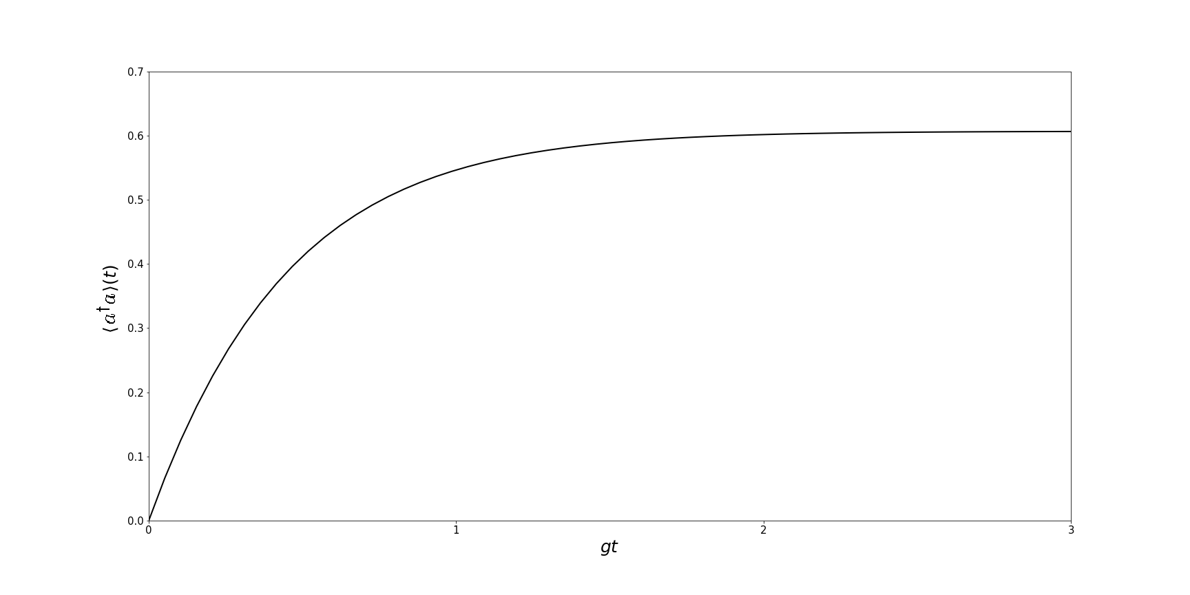
Figure 4: The photon number. The mean occupation number $\left\langle a^{{\dagger}}a\right\rangle(t)$, considering the same parameters used in Fig. $2$, together with $\mathcal{C}/g=0.35$, $r/g=92$ and $\gamma/g=0.5$, leading to $\mathcal{A}/g=736$. We consider the cavity initially in the vacuum state and the atoms prepared in their excited states.

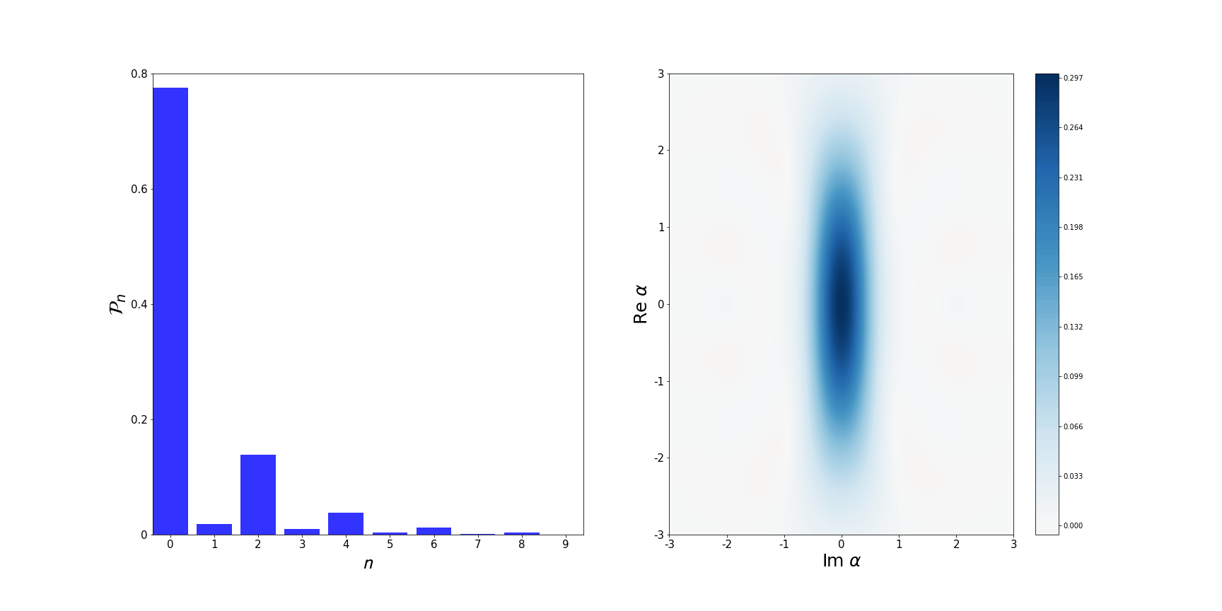
(a)

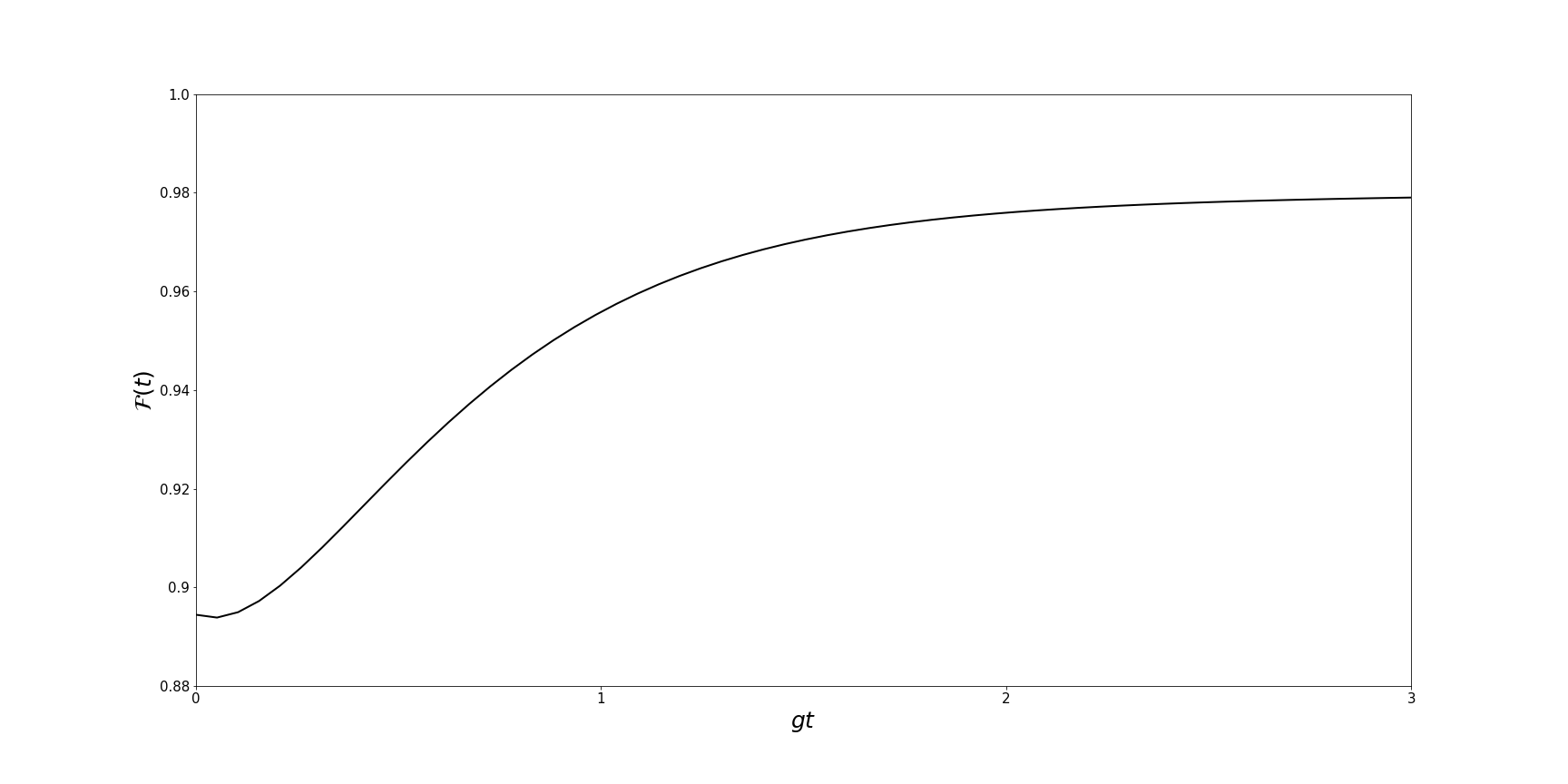
(b)

Figure 5: Squeezed vacuum laser. (a), The photon number distribution $\mathcal{P}_{n}$ and the phase space projection of the Wigner function of the produced laser state for $gt=4$, and (b) the fidelity of the evolved laser state against $gt$. We use the same parameters of Fig. 4.

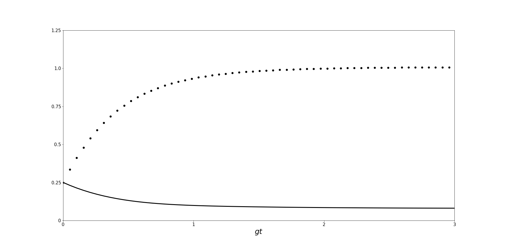
Figure 6: The variances, $\left(\Delta X_{1}\right)^{2}(t)$ (solid line) and $\left(\Delta X_{2}\right)^{2}(t)$ (dotted line) of the generated laser state against $gt$, using the same parameters of Fig. 4.

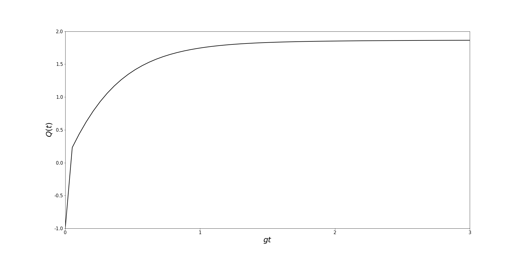
Figure 7: The nonclassicality. The Mandel $Q_{M}$ parameter for the laser state against $gt$, using the same parameters of Fig. 4

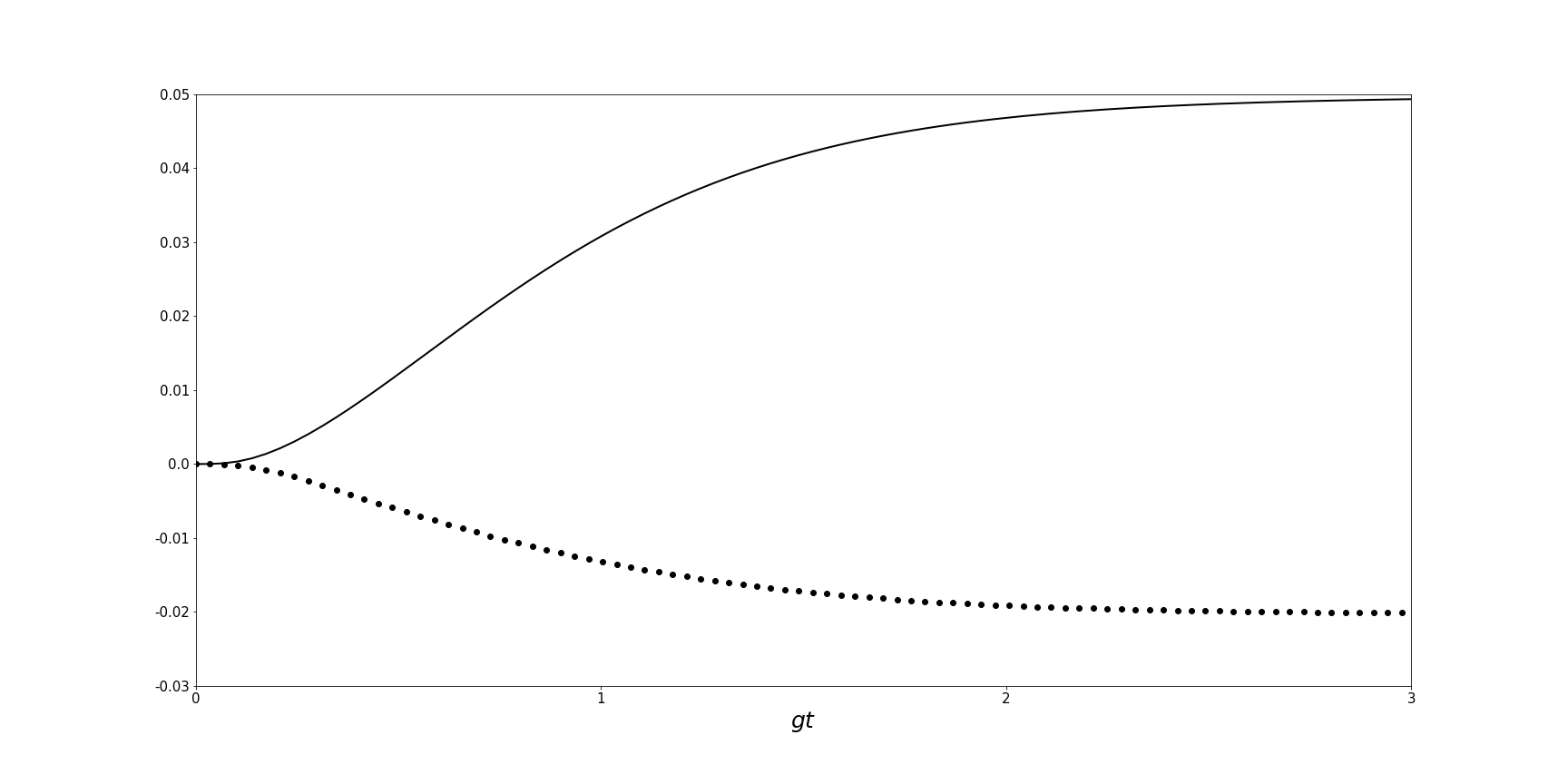
Figure 8: The absence of diffusion. Off-diagonal matrix elements $\rho_{0,8}(t)$ and $\rho_{4,6}(t)$ against $gt$, using the same parameters of Fig. 4.

We note that for $\kappa=0$ we immediately recover the usual Fock basis states from Eq. (9) and the usual coherent state from Eq. (11). In Fig. 3(a) we show the photon number distribution $\mathcal{P}_{n}$ and a phase-space plot of the uncertainties of the laser state given by Eq. (11), using $\alpha=0.18$ and $r=\operatorname*{Tanh}^{-1}\kappa=0.69$, and considering $\kappa=0.6$ as in Fig. 2. The obtained squeezed vacuum displays a good agreement with the ideal squeezed vacuum $S(r=0.69)\left|0\right\rangle$, whose photon distribution and projection of the Wigner distribution in phase space is shown in Fig. 3(b), where $S$ stands for the well-known squeeze operator

$$S(\xi)=\exp\left[\xi^{\ast}a^{2}-\xi\left(a^{{\dagger}}\right)^{2}\right],$$ (12)

with $\xi=re^{i\varphi}$, $r$ being the degree of squeezing and $\varphi$ the squeezing direction in phase space [33, W], here with $\varphi=0$. The produced laser state deviates slightly from the ideal squeezed vacuum as indicated by the populations of the odd Fock states. We point out that, the squeezed vacuum with squeezing factor $r=\tanh^{-1}\kappa$, is an eigenstate of $A$ with null eigenvalue, as required by the engineering reservoir technique.

IV The master equation for the squeezed vacuum laser

From the isomorphism we have established, and following the footsteps of the conventional laser theory, we can derive the master equation describing the dynamics of the cavity field when interacting with a pumped atomic sample, through the effective Hamiltonian (5), and the environment. This master equation is given by

$$\dot{\rho}=\mathcal{L}_{\mathcal{A}}\rho+\mathcal{L}_{\mathcal{B}}\rho+\mathcal{L}_{\mathcal{C}}\rho,$$ (13)

where the Lindbladians accounting for gain, saturation and cavity loss, obey the expressions

$$\mathcal{L}_{\mathcal{A}}\rho =\frac{\mathcal{A}}{2}\left(2A^{{\dagger}}\rho A-AA^{{\dagger}}\rho-\rho AA^{{\dagger}}\right),$$ (14a)

$$\mathcal{L}_{\mathcal{B}}\rho =\frac{\mathcal{B}}{2}\left[\frac{1}{4}AA^{{\dagger}}\left(AA^{{\dagger}}\rho+3\rho AA^{{\dagger}}\right)\right.$$

$$\left.+\frac{1}{4}\left(\rho AA^{{\dagger}}+3AA^{{\dagger}}\rho\right)AA^{{\dagger}}\right.$$

$$\left.-A^{{\dagger}}\left(AA^{{\dagger}}\rho+\rho AA^{{\dagger}}\right)A\right]+...,$$ (14b)

$$\mathcal{L}_{\mathcal{C}}\rho =\frac{\mathcal{C}}{2}\left(2A\rho A^{{\dagger}}-A^{{\dagger}}A\rho-\rho A^{{\dagger}}A\right).$$ (14c)

The coefficients for gain $\mathcal{A}=2R\left(g/\gamma\right)^{2}$, saturation $\mathcal{B}=4\mathcal{A}\left(g/\gamma\right)^{2}$, and loss $\mathcal{C}=\omega/Q$, are defined from the atomic pumping rate $R=Kp$, $K$ being the total atomic injection rate and $p$ the probability for the atomic laser excitation, the Rabi frequency $g$, and effective atomic decay rate $\gamma$, and the cavity quality factor $Q$. The Lindbladian for saturation in Eq. (14b) is given only up to 4-th order in $g$. The isomorphism then assures us that the squeezed vacuum state in Eq. (11) follows directly from the competition between amplification ($\mathcal{A}$) and dissipation ($\mathcal{C}$), mediated by the the saturation of the cavity field excitation ($\mathcal{B}$), described by the master equation (13). Far above threshold, when $\mathcal{A\gg C}$, the far from equilibrium steady state of the cavity field is given by Eq. (11).

We note here that unlike what happens with engineered reservoirs, we do not have a term in Eq. (13) (similar to the Lindbladian for $a^{{\dagger}},a$ in Eq. (2)), that acts to introduce error in the laser mechanism. This is indeed a remarkable bonus for our method, in which the only source of errors stems from the engineering of the effective Hamiltonian (5). By limiting the time interval of the laser operation such that $gt=7$, the errors coming from the engineered protocol must, however, be small as we have seen from Fig. 2.

To further support our results coming from the isomorphism —that the laser resulting from the atom-field interaction described by the effective Hamiltonian (5) is indeed the squeezed vacuum—, in what follows we numerically analyze the construction, step by step, of such a cavity field steady state. To do that, we numerically simulate the passage of a dense flux of atoms through an excitation region where each atom has a probability $p$ of being excited to the level $|e\rangle$ before entering the cavity. Considering that this flux has a regular pump rate, $K$, we can say that the number of atoms passing through a time $\Delta t$ is equal to $K\Delta t$, as much as the average number of excited atoms that reach the cavity is $N=k\Delta t$, where $k=pK$. The atoms arrive successively in the cavity so that the atom-field interaction described by (5) still apllies collectively, since it has being developed individually. The first atom finds the cavity field in its initial vacuum state $\rho(0)$, leading it to the state $\rho(t)$, with $t=1/k$. After its passage through the cavity, we compute the reduced density operator for the field state by tracing over the atomic degrees of freedom. The second atom then finds the cavity in this reduced state, leading it to another reduced state at time $2t$, and so on until the time $Nt$, each step being described by the equation

$$\dot{\rho}_{i+1}(t)=k\left[\rho(t_{i+1})-\rho(t_{i})\right]=-i\left[H_{eff}(t_{i}),\rho(t_{i})\right]$$ (15)

$$+\left(C/2\right)\left[2A\rho(t_{i})A^{{\dagger}}-A^{{\dagger}}A\rho(t_{i})-\rho(t_{i})A^{{\dagger}}A\right]$$ (16)

$$+\left(\gamma/2\right)\left(2\sigma_{-}\rho(t_{i})\sigma_{+}-\sigma_{+}\sigma_{-}\rho(t_{i})-\rho(t_{i})\sigma_{+}\sigma_{-}\right)\text{.}$$ (17)

We next analyze the laser state derived from Eq. (17), by comparing it with the squeezed vacuum state defined in Eq. (11), which by its turn comes from Eq. (13). All the following figures consider the same parameters used in Fig. 2 to validate the effective interaction in Eq. (5), together with the choices $\mathcal{C}/g=0.35$, $r/g=92$ and $\gamma/g=0.5$, which lead to the rate $\mathcal{A}/g=736$.

In Fig. 4 we plot the mean occupation number $\left\langle a^{{\dagger}}a\right\rangle(t)$ of the laser state resulting from Eq. (17). We verify that the mean occupation number reaches the steady value $\left\langle a^{{\dagger}}a\right\rangle(t)=0.62$ for $gt\approx 3$, long before the validity of the effective Hamiltonian is compromised, for $gt\approx 7$. This steady excitation is in good agreement with that predicted by Eq. (11), given by $\left\langle a^{{\dagger}}a\right\rangle=0.56$, about $10\%$ less than the numerical simulation. The value $gt\approx 3$ follows after the passage of $1734$ atoms through the cavity.

In Fig. 5(a) we present the photon number distribution $\mathcal{P}_{n}$ and the phase space projection of the Wigner function of the laser state following from Eq. (17), for $gt=4$. We again verify a good agreement with the ideal squeezed vacuum state as it becomes clear from Fig. 5(b) where the fidelity $\mathcal{F}=\operatorname*{Tr}\rho S(\xi)\left|0\right\rangle\left\langle 0\right|S^{{\dagger}}(\xi)$ of the state $\rho$ coming from Eq. (17) is plotted against $gt$, regarded to the ideal squeezed vacuum $S(\xi)\left|0\right\rangle$ in Eq. (11). We note that the fidelity already starts from a high value due to the large population of the state in the squeezed vacuum field. The plot if Fig. 5(a) also indicates that our laser has zero diffusion; if we had non-zero diffusion, the elliptical projection should circulate around the origin of the phase space, as occurs with the coherent state of the conventional laser theory [33].

In Figs. 6 we plot the variances $\left(\Delta X_{1}\right)^{2}(t)$ (solid line) and $\left(\Delta X_{2}\right)^{2}(t)$ (dotted line), against $gt$, of the laser state coming from Eq. (17), showing that these variances approaches the values $\left(\Delta X_{1}\right)_{(S(\xi)\left|0\right\rangle)}=\frac{e^{-2r}}{4}=0.06$ and $\left(\Delta X_{2}\right)_{(S(\xi)\left|0\right\rangle)}=\frac{e^{2r}}{4}=0.98$, computed from the squeezed vacuum state in Eq. (11). In Fig. 7 we plot the Mandel parameter $Q_{M}=\left(\left\langle n^{2}\right\rangle-\left\langle n\right\rangle^{2}\right)/\left\langle n\right\rangle-1$ for the laser state, showing that for $gt\approx 2$ we reach a stationary value around $Q=2\cosh(\lvert r\rvert)-1=2.1,$ as expected for the ideal squeezed vacuum state. Finally, in Fig. 8 we plot the off-diagonal matrix elements $\rho_{0,8}(t)$ and $\rho_{4,6}(t)$, which demonstrate, together with Fig. 5(a), that the phase coherence is preserved due to the absence of phase diffusion of our squeezed vacuum laser, since $A\left|\alpha\right\rangle_{A}$ $=0$; otherwise these matrix elements would decay to zero.

V Conclusion

We have presented a method to produce a squeezed vacuum laser with zero diffusion. This method is based on merging together the reservoir engineering technique with the laser theory. The reservoir engineering demands us to build up an effective interaction between the the system whose state we want to protect (the cavity field) and an auxiliary system (the laser active medium), of the form of Eq. (3), $\chi\left(A\sigma_{+}+A^{{\dagger}}\sigma_{-}\right)$, with the laser steady state being an eigenstate of $A$ with null eigenvalue: $A\left|\Psi\right\rangle=0$. The effective interaction must enable the construction of an isomorphism between the field operators in the effective $\left(A^{{\dagger}},A\right)$ and the Jaynes-Cummings $\left(a^{{\dagger}},a\right)$ Hamiltonians. The isomorphism is carried out by building a basis state $\left\{\left|n\right\rangle_{A}\right\}$ for the operators $A^{{\dagger}},A$ similar to the Fock basis state $\left\{\left|n\right\rangle\right\}$ for $a^{{\dagger}},a$. The laser theory, by its turn, provides the mechanism by which the cavity mode is fed by the stimulated emission of the active medium when subjected to linear amplification, in addition to inducing a saturation whichresults in a far-from-equilibrium steady state.

Our method has an advantage over the reservoir engineering, in which we cannot, evidently, eliminate the environment (described by the Lindbladian for $a^{{\dagger}},a$ in Eq. (2)) that acts to introduce errors in the action of the artificially constructed reservoir (described by the Lindbladian for $A^{{\dagger}},A$). In our method, this does not occur, the only source of errors being the protocol for building up the effective interaction, based on the adiabatic elimination of fast variables, which is also present in reservoir engineering. This is a very unique aspect of our method, which shows that the association of reservoir engineering with the laser mechanism results in both a more robust protocol than the reservoir engineering (since the Lindbladian for $a^{{\dagger}},a$ is absent) and also an unconventional laser field described by a nonclassical coherence-preserving state.

In addition to the many applications we have already listed for a zero linewidth laser, we observe that a squeezed vacuum laser may be useful for high-resolution interferometry, a timely topic due to the newly emerging field of gravitational-wave interferometry. Moreover, the present method challenges us to design effective interactions leading to other nonclassical laser states, as for example steady superposition states. This challenge can leads us to a new chapter regarding the preparation of nonclassical steady states, which could be useful for a variety of fundamental and technological applications.

Acknowledgements

FON and MHYM would like to thank CAPES and INCT-IQ for support.

References

- [1] A. L Schawlow and C. Townes, Physical Review 112, 6 (1940).
- [2] T. H. Maiman, Nature 187, 493 (1960).
- [3] H. Haken, Laser theory (Springer, Berlin, Heidelberg, 1984).
- [4] M. Sargent III, M. O. Scully, and W. E. Lamb, Laser Physics (Addison Wesley 1974); M. O. Scully and W. E. Lamb, Phys. Rev. 159, 208 (1967).
- [5] M. Lax, and W. H. Louisell, Phys. Rev. 185, 568 (1969).
- [6] B. Baseia and H. M. Nussenzveig, Semiclassical Theory of Laser Transmission Loss, Optica Acta: International Journal of Optics 31, 39 (1984).
- [7] Y. M. Golubov, and I. V. Sokolov, Sov. Phys. JETP 60, 234 (1984); Y. Yamamoto et al., Phys. Rev. 34, 4025 (1986); F. Haake et al., Phys. Rev. 40, 7121 (1989); J. Bergou et al., Opts. Commun. 72, 82 (1989).
- [8] W. D. Phillips, Rev. Mod. Phys. 70, 721 (1998); S. Chu, Rev. Mod. Phys. 70, 685 (1998); C. N. Cohen-Tannoudji, Rev. Mod. Phys. 70, 707 (1998).
- [9] W. Ketterle, Rev. Mod. Phys. 74, 1131 (2002); E. A. Cornell and C. E. Wieman, Rev. Mod. Phys. 74, 875 (2002).
- [10] A. Ashkin, Phys, Rev. Lett. 24, 156 (1970); A. Ashkin et al., Optics letters 11, 288 (1986); A. Ashkin et al., Nature 330, 769 (1987); A. Ashkin and J. M. Dziedzic, Science 235, 1517 (1987).
- [11] D. Strickland and G. Mourou, Opt. Comm. 55, 447 (1985); P. Maine et al., IEEE Journal of Quantum electronics 24, 398 (1988).
- [12] V. V. Dodonov, J. Opt. B 4, R1(2002).
- [13] C. M. Caves, Phys. Rev. D 28, 1693 (1981).
- [14] C. M. Caves, Phys. Rev. D 23, 1693 (1981).
- [15] P. Meystre and M. O. Scully, Eds. Quantum Optics, Experimental Gravitation and Measurement Theory, Plenum, New York.
- [16] B. P. Abbott et al., Phys. Rev. Lett. 116, 061102 (2016).
- [17] J. H. Shapiro, Opt. Lett. 5, 351 (1980).
- [18] H. Yonezawa and A. Furusawa, Opt. Spectrosc. 108, 288 (2010); R. Ukai, N. Iwata, Y. Shimokawa, S. C. Armstrong, A. Politi, J.-i. Yoshikawa, P. van Loock, and A. Furusawa, Phys. Rev. Lett. 106, 240504 (2011).
- [19] G. Brida, M. Genovese, and I. R. Berchera, Nat. Photonics 4, 227 (2010); V. D’ambrosio, N. Spagnolo, L. Del Re, S. Slussarenko, Y. Li, L. C. Kwek, L. Marrucci, S. P. Walborn, L. Aolita, and F. Sciarrino, Nat. Commun 4, 2432 (2013).
- [20] A. Aspect et al., Phys. Rev. Lett. 49, 91 (1982); P. G. Kwiat et al., Phys. Rev. Lett. 75, 4337 (1995).
- [21] M. Nielsen and I. Chuang, Quantum Computation and Quantum Information (Cambridge University Press, 2000).
- [22] K. Vogel et al., Phys. Rev. Lett. 71, 1816 (1993); Ch. Roos et al., Phys. Rev. Lett. 83, 4713 (1999); C. J. Villas-Bôas et al., Phys. Rev. A 68, 053808 (2003); F. O Prado et al., EPL 107 13001 (2014); R. F. Rossetti et al., Phys. Rev. A 90, 033840 (2014); Erratum Phys. Rev. A 93, 069904 (2016); G. D. de Moraes Neto et al., Phys. Rev. A 90, 062322 (2014).
- [23] O. Gamel and D. F. V. James, Phys. Rev. A 82, 052106 (2010); D. F. V. James and J. Jerke, Can. J. Phys. 85, 625 (2007).
- [24] G. D. de Moraes Neto et al., EPL 103, 43001 (2013); ibid., Phys. Rev. A 85, 052303 (2012); ibid., Phys. Rev. A 84, 032339 (2011); S. B. Zheng, and G. C. Guo, Phys. Rev. Lett. 85, 2392 (2000); R. L. Rodrigues et al., Phys. Rev. A 74, 063811 (2006).
- [25] J. F. Poyatos et al., Phys. Rev. Lett. 77, 4728 (1996).
- [26] G. D. de Moares Neto et al., Phys. Rev. A 90, 062322 (2014); R. F. Rossetti et al., Phys. Rev. A 90, 033840 (2014); F. O. Prado et al., EPL 107, 13001 (2014); F. O. Prado et al., Phys. Rev. Lett. 102, 073008 (2009); L. C. Celeri et al., J. Phys. B 41, 085504 (2008).
- [27] S. Haroche, Rev. Mod. Phys. 85, 1083 (2013).
- [28] D. J. Wineland, Rev. Mod. Phys. 85, 1103 (2013).
- [29] T. Ozawa et al., Rev. Mod. Phys. 91, 015006 (2019).
- [30] A. M. Steane, Quantum Error Correction, in H. K. Lo, S. Popescu, and T. P. Spiller, editor, Introduction to Quantum Computation and Information, page 184. Word Scientific, Singapore, 192331 (2011).
- [31] S. Huang, T. Zu, M. Liu, and W. Huang, Sci. Rep. 7, 41988 (2017); M. A. Tran, D. Huang, and J. E. Bowers, APL Photon. 4, 111101 (2019).
- [32] L.-A. Wu, H. J. Kimble, J. L. Hall, and H. Wu, Phys. Rev. Lett. 57, 2520 (1986).
- [33] M. Scully and M. S. Zubairy, Quantum Optics (Cambridge University Press, New York, 1997); D. F. Walls and G. J. Milburn, Quantum Optics (Springer-Verlag, Berlin, 1994).
- [34] R. E. Slusher, L. W. Hollberg, B. Yurke, J. C. Mertz, and J. F. Valley, Phys. Rev. Lett. 55, 2409 (1985).
- [35] C. J. Villas-Bôas, N. G. de Almeida, R. M. Serra, and M. H. Y. Moussa, Phys. Rev. A 68, 061801(R) (2003); N. G. de Almeida, R. M. Serra, C. J. Villas-Bôas, and M. H. Y. Moussa, Phys. Rev. A 69, 035802 (2004); R. M. Serra, C. J. Villas-Bôas, N. G. de Almeida, and M. H. Y. Moussa, Phys. Rev. A 71, 045802 (2005); F. O. Prado, N. G. de Almeida, M. H. Y. Moussa, and C. J. Villas-Bôas, Phys. Rev. A 73, 043803 (2006).
- [36] O. Gamel and D. F. V. James, Phys. Rev. A 82, 052106 (2010); D. F. V. James and J. Jerke, Can. J. Phys. 85, 625 (2007).
- [37] G. D. M. Neto, M. A. de Ponte, M. H. Y. Moussa, Phys. Rev. A 85, 052303 (2012); G. D. de Moraes Neto, M. A. de Ponte and M. H. Y. Moussa, EPL 103, 43001 (2013); F O Prado, W Rosado, A M Alcalde and M H Y Moussa, J. Phys. B: At. Mol. Opt. Phys. 46, 205501 (2013); W. Rosado, G. D. de Moraes Neto, F. O. Prado, and M. H. Y. Moussa, J. Mod. Opt. 62, 1561 (2015); R. F. Rossetti, G. D. de Moraes Neto, J. Carlos Egues and M. H. Y. Moussa, EPL 115, 53001 (2016).
- [38] A. D. Boozer, Ph.D. thesis, California Institute of Technology, 2005. Ibid. Phys. Rev. A 78, 033406 (2008).
- [39] C. S. Muñoz and D. Jaksch, arXiv:2008.02813v2 [quant-ph] 23 Apr 2021.