$\mu$-distortion around stupendously large primordial black holes

Abstract

In a variety of mechanisms generating primordial black holes, each black hole is expected to form along with a surrounding underdense region that roughly compensates the black hole mass. This region will propagate outwards and expand as a shell at the speed of sound in the homogeneous background. Dissipation of the shell due to Silk damping could lead to detectable $\mu$-distortion in the CMB spectrum. While the current bound on the average $\mu$-distortion is $\left|\bar{\mu}\right|\lesssim 10^{-4}$, the standard $\Lambda$CDM model predicts $\left|\bar{\mu}\right|\sim 10^{-8}$, which could possibly be detected in future missions. It is shown in this work that the non-observation of $\bar{\mu}$ beyond $\Lambda$CDM can place a new upper bound on the density of supermassive primordial black holes within the mass range $10^{6}M_{\odot}\lesssim M\lesssim 10^{15}M_{\odot}$. Furthermore, black holes with initial mass $M\gtrsim 10^{12}M_{\odot}$ could leave a pointlike distortion with $\mu\gtrsim 10^{-8}$ at an angular scale $\sim 1^{\circ}$ in CMB, and its non-observation would impose an even more stringent bound on the population of these stupendously large primordial black holes.

I Introduction

Primordial black holes (PBHs) are hypothetical black holes formed in the early universe before any large scale structures and galaxies. Unlike astrophysical black holes formed by the collapse of dying stars, PBHs are speculated to be formed from large perturbations during the radiation era (typically within the first few seconds after inflation ends) and can have a mass ranging from the Planck mass ($\sim 10^{-5}\ \text{g})$ to many orders of magnitude larger than the solar mass ($M_{\odot}\sim 10^{33}\ \text{g}$). The reader is referred to ref. Carr et al. (2020) for an up-to-date review on PBHs in regard of the mechanisms of formation and the current observational constraints on their population in our universe.

PBHs have drawn much attention recently because they could be responsible for the discoveries announced by the LIGO/Virgo Collaboration Bird et al. (2016); Sasaki et al. (2016); Clesse and García-Bellido (2017). In the past few years, LIGO/Virgo detected about 50 signals Abbott et al. (2019, 2020a), most of which are believed to be gravitational waves from inspiraling and merging black holes of mass $\mathcal{O}(10-100)M_{\odot}$. The origin of these black holes is so far unknown. Some of them have masses larger than what one would expect in stellar models. For example, the surprising event GW190521 involves a black hole of mass 85$M_{\odot}$ Abbott et al. (2020b), which lies within the “pair instability mass gap” Woosley (2017); Belczynski et al. (2016); Spera and Mapelli (2017); Giacobbo et al. (2018). Hence the detection of the LIGO/Virgo black holes could be a hint of the existence of PBHs.

PBHs could also provide an explanation for supermassive black holes at the center of most galaxies Lynden-Bell (1969); Kormendy and Richstone (1995). These black holes have masses of $\mathcal{O}(10^{6}-10^{10})M_{\odot}$, and observations of quasars indicated that some of them were already present at high redshifts. For example, a black hole of mass $M\sim 10^{9}M_{\odot}$ was discovered recently from the most distant quasar ever observed at redshift $z\approx 7.642$ Wang et al. (2021). The existence of these black holes greatly challenges the conventional mass accretion model of astrophysical black holes, as it is unable to fully explain the significant growth from stellar seeds Haiman (2004). PBHs, on the other hand, can be a natural candidate of these supermassive objects because they could have a large mass when they were born Rubin et al. (2001); Bean and Magueijo (2002); Duechting (2004); Carr and Silk (2018).

Yet another fascinating possibility, which has been under extensive investigation for a long time, is that PBHs constitute (a major part of) the dark matter. Observational bounds imposed by microlensing, dynamical and astrophysical effects are stringent in most of the mass range (see, e.g., refs. Carr et al. (2020); Carr and Kuhnel (2020) and references therein), but the window $\mathcal{O}(10^{17}-10^{23})\text{g}$ is open, hence can still allow small PBHs to account for all dark matter.

In the present work, we shall discuss a possible physical effect accompanied by the production of PBHs: $\mu$-distortion in the spectrum of the cosmic microwave background (CMB) around each PBH. Such an effect can arise in a variety of mechanisms of PBH formation that require the total energy excess of the perturbation to (approximately) vanish as the spacetime goes asymptotically flat FRW. This requirement is not only satisfied for PBHs from, e.g., topological defects or phase transitions Hawking (1989); Polnarev and Zembowicz (1991); Garriga and Vilenkin (1993); Caldwell and Casper (1996); Hawking et al. (1982); Rubin et al. (2000); Khlopov et al. (2005); Garriga et al. (2016), but could also be fulfilled in the most popular scenario, where PBHs are formed by mass overdensities that collapse upon Hubble reentry after inflation. If this condition is met, there would be a compensating underdense region surrounding each PBH. After black hole formation, the underdense region will propagate outwards as a shell at the speed of sound. If the black hole is sufficiently massive, the corresponding sound shell can have a wave energy so large that its dissipation due to Silk damping would lead to detectable $\mu$-distortion in the CMB spectrum.

It is the task of this paper to estimate the magnitude of the distortion and to investigate how it could be used to constrain the PBH density. As we will see, while the resulting constraints could be applied to the mass range $M\gtrsim 10^{6}M_{\odot},$ they would be particularly interesting for PBHs with an initial mass $M\gtrsim 10^{11}M_{\odot}$, which we call “stupendously large PBHs” following ref. Carr et al. (2021). Our main results are shown in fig. 3.

The rest of the paper is organized as follows. In section II we discuss the evolution of the sound shell surrounding each PBH, how its dissipation by Silk damping can lead to $\mu$-distortion in CMB, and how the distortion could impose constraints on PBHs with the help of future observations. Conclusions are summarized and discussed in section III. We set $c=\hbar=G=k_{B}=1$ throughout the paper.

II $\mu$-distortion around PBHs

In the most popular and perhaps the most natural scenario discussed in the literature, PBHs could form by some rare overdense clumps in space that are from sufficiently large curvature perturbations at small scales. These perturbations can be attained by manipulating the inflationary potential Ivanov et al. (1994); Garcia-Bellido et al. (1996); Kawasaki et al. (1998); Yokoyama (1998); Garcia-Bellido and Ruiz Morales (2017); Hertzberg and Yamada (2018). After inflation ends, these clumps could overcome pressure and collapse into black holes as they reenter the Hubble horizon. In the so-called “compensated” model Harada and Carr (2005); Carr and Harada (2015); Harada et al. (2015), the total energy excess of the perturbation is zero, and the spacetime away from the perturbation is flat FRW. This implies there should be a compensating underdensity around the clump (see, e.g., refs Germani and Musco (2019); Kehagias et al. (2019) for examples of the density profile from various power spectra of curvature perturbations). Therefore, each of the resulting black holes is surrounded by an underdense region, whose energy deficit compensates the black hole mass. This region will then propagate outwards as a spherical sound wave packet, or, a sound shell. As the shell sweeps through the background, the fluid density between the black hole and the shell goes back to FRW. Illustrations of this process are shown in fig. 1. Dissipation of the shell due to photon diffusion during the so-called $\mu$-era can release energy into the background, generating $\mu$-distortion in the background photons, and may thus be seen in CMB.

A similar picture can be applied to mechanisms of PBH formation involving topological defects (such as cosmic strings and domain walls) or phase transition bubbles Hawking (1989); Polnarev and Zembowicz (1991); Garriga and Vilenkin (1993); Caldwell and Casper (1996); Hawking et al. (1982); Rubin et al. (2000); Khlopov et al. (2005); Garriga et al. (2016). This is because, since the global energy is conserved with the formation of these objects, an energy excess that eventually turns into a black hole should be compensated by a nearby energy deficit. We first noticed this effect in our previous studies on PBHs formed by vacuum bubbles and spherical domain walls that nucleate during inflation Deng et al. (2017); Deng and Vilenkin (2017); Deng (2020a), then in refs. Deng et al. (2018); Deng (2020b) we further investigated the spectral distortions produced by the evolution of the deficit in our specific models. It was later realized that this effect can be generalized to a variety of PBH mechanisms, which can be used to constrain the PBH density in general.

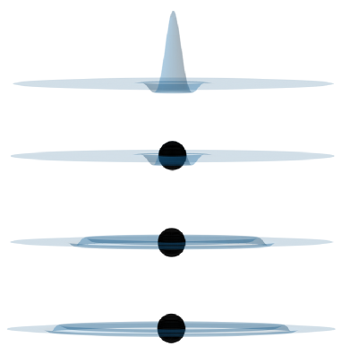
Figure 1: Illustration of the formation of sound shell around a PBH. In this example the PBH is formed by the collapse a large overdense clump, which is surrounded by an underdense region. After the black hole is formed, the underdense region expands as a shell (shown as a ring here). The shell consists of an underdense and an overdense layer, which is a typical feature of a spherical sound wave packet Landau and Lifshitz (2013). As the shell sweeps through, the fluid density between the black hole and the shell goes back to FRW.

II.1 Dissipation of sound shell

Before estimating the magnitude of the distortion, let us first describe how the sound shell gets dissipated by photon diffusion in plasma. More details can be found in the appendix. Roughly speaking, the black hole is formed at a time $t_{M}$ when the Hubble horizon mass is comparable to the black hole mass Carr et al. (2020), i.e.,

$$t_{M}\sim M.$$ (1)

If the underdensity surrounding the black hole is of a scale comparable to the black hole horizon ($2M$), then since the total energy excess is assumed to vanish, the density contrast $\delta$ in the underdense region should satisfy $\mathcal{O}(10)\rho_{r}(t_{M})\delta M^{3}+M=0$, where $\rho_{r}(t)=3/32\pi t^{2}$ is the background FRW density. This gives $\left|\delta\right|\sim 1$. As the underdensity propagates outwards in the form of a shell, $\left|\delta\right|$ becomes smaller and smaller, and the shell can thus be described as a spherical sound wave packet. According to hydrodynamics (and the appendix), the sound wave energy density is given by $\rho_{s}=\rho_{r}\delta^{2}/4$, hence the sound wave energy of the underdense shell $E_{s}(t)$ at $t_{M}$ is $E_{s}(t_{M})=\mathcal{O}(10)\rho_{s}(t_{M})M^{3}\sim M$.

If there is no photon diffusion, the thickness of the shell $D$ simply gets stretched by cosmic expansion:

$$D(t)\sim\left(Mt\right)^{1/2},$$ (2)

and the sound wave energy of the shell is $E_{s}(t)\sim M^{2}/D\propto t^{-1/2}$, which simply gets redshifted over time. Due to photon diffusion, the photon-electron fluid can be effectively described by an imperfect fluid with a shear viscosity Weinberg (1971, 2008); Pajer and Zaldarriaga (2013). By the appendix, the thickness of the shell $S$ gets further smeared, and can be estimated as

$$S(t)\sim\left(D^{2}+\Lambda^{2}\right)^{1/2},$$ (3)

where $\Lambda(t)$ is the physical scale of photon diffusion (the typical distance traveled by a photon till the time $t$), and is given by

$$\Lambda(t)\approx\left(\frac{t}{\sigma_{T}n_{e}}\right)^{1/2}\approx\left(\frac{t}{10^{10}\text{s}}\right)^{3/4}t^{1/2}\left(10^{12}M_{\odot}\right)^{1/2}.$$ (4)

Here, $\sigma_{T}$ is the Thomson cross-section and $n_{e}$ is the electron density, and we have expressed $\Lambda$ in a form convenient for our computations below. By eq. (49) in the appendix, the sound wave energy of the shell becomes

$$E_{s}(t)\sim\left(\frac{D}{S}\right)^{3}\frac{M^{2}}{D}\sim\left[1+\left(\frac{t}{10^{10}\text{s}}\right)^{3/2}\left(\frac{M}{10^{12}M_{\odot}}\right)^{-1}\right]^{-3/2}M^{3/2}t^{-1/2},$$ (5)

which gets damped over time by a factor of $(D/S)^{3}$ compared to the case without viscosity. Therefore, as the sound shell expands, part of its wave energy is dumped into the space behind it, heating up the photons there. This energy release could lead to a unique type of spectral distortion in CMB, which will be the topic of the next subsection.

II.2 $\mu$-distortion

CMB photons came from the last scattering surface with comoving radius $\sim 10\ \text{Gpc}$, at a time $\sim 10^{12}-10^{13}\ \text{s}$ after inflation ends. During this time, photons decoupled from electrons and began to travel across the transparent universe in all directions. Several generations of detectors have shown with high precision that the CMB spectrum is extremely close to a black-body of temperature $T\approx 2.7\ \text{K}$. However, tiny deviations from the black-body spectrum, commonly referred to as spectral distortions, could arise from plenty of physical processes. Discovery of spectral distortions would then provide valuable information of the pre-recombination universe.

A typical example of spectral distortions in CMB is known as the $\mu$-distortion, which is generated by the mix of photons with different temperatures during the $\mu$-era, when $6\times 10^{6}\ \text{s}\approx t_{th}\lesssim t\lesssim t_{\mu}\approx 10^{10}\ \text{s}$. At time $t<t_{th}$, photons are completely thermalized and have a perfect black-body spectrum. During the $\mu$-era, photon number changing processes such as bremsstrahlung and double Compton scattering become ineffective, while the Compton process still allows photons to reach equilibrium with the background plasma. As a result, when there is energy released into the background, the mix of photons with different temperatures would lead to a spectrum with nonzero chemical potential $\mu$ Sunyaev and Zeldovich (1970); Daly (1991); Barrow and Coles (1991); Hu and Silk (1993).

Energy release in the early universe can occur in various possible mechanisms. A well known example is the Silk damping Silk (1968), where small-scale perturbations are smoothed out by photon diffusion before the time of recombination. In our scenario, the Silk damping of the sound shell constantly injects heat into the background as the shell sweeps through space. During the $\mu$-era, the comoving radius of the shell (which is also approximately the comoving sound horizon) ranges from $r_{th}\sim 0.1\ \text{Mpc}$ to $r_{\mu}\sim 5\ \text{Mpc}$ . On the other hand, the comoving scale of photon diffusion at the time of recombination is $\lambda_{rec}\sim 50\ \text{Mpc}$. Because Silk damping continues to work after the $\mu$-era until recombination, $\lambda_{rec}\gg r_{\mu}$ means each black hole is at the center of a region of scale $\lambda_{rec}$ that has a distorted spectrum with a uniform $\mu$. Such a region will be referred to as a “Silk region”, and its projection on the last scattering surface will be called a “Silk patch”. Let us now estimate the $\mu$-distortion around a single black hole within a Silk region.

In the presence of energy release, the dimensionless chemical potential $\mu$ ($\equiv-\mu_{th}/T$, where $\mu_{th}$ is the thermodynamic chemical potential and $T$ is the background temperature) can be obtained by Sunyaev and Zeldovich (1970); Daly (1991); Barrow and Coles (1991); Hu and Silk (1993)

$$\mu\approx 1.4\frac{\Delta\rho_{s}}{\rho_{r}},$$ (6)

where $\Delta\rho_{s}$ is the density of the released energy and $\rho_{r}$ is the background radiation density. In calculating $\Delta\rho_{s}$ from $E_{s}$, we ought to consider only the effect of dissipation, and not the dilution from cosmic expansion. In the explicit expression of $E_{s}$ in eq. (5), the effect of cosmic expansion is from $t^{-1/2}$. Therefore, as the sound shell sweeps through a sphere at time $t$, the total released energy can be estimated as

$$\Delta E_{s}(t)\sim\frac{\text{d}\left(E_{s}t^{1/2}\right)}{\text{d}t}t^{-1/2}\Delta t,$$ (7)

where $\Delta t\sim S/c_{s}$ is the time it take for the shell to pass through the sphere ($c_{s}=1/\sqrt{3}$ is the speed of sound). Since the volume of the shell is $\sim 4\pi(2c_{s}t)^{2}S$, where $2c_{s}t$ is the shell’s physical radius, we have

$$\Delta\rho_{s}(t)\sim\frac{\Delta E_{s}}{4\pi(2c_{s}t)^{2}S}.$$ (8)

A sketch of this process is shown in fig. 2. Now the $\mu$-distortion produced at time $t$ can readily be expressed as

$$\mu(t)\approx 4.85\frac{\text{d}\left(E_{s}t^{1/2}\right)}{\text{d}t}t^{-1/2}.$$ (9)

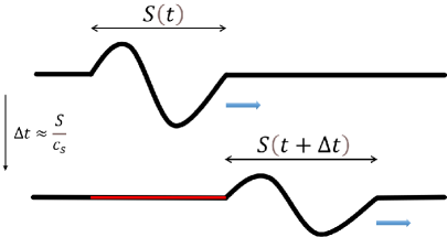
Figure 2: Sketch of the radiation fluid’s density profile along the radius near the shell at two moments $t$ and $t+\Delta t$. The shell consists of an underdense and an overdense layer, which is a typical feature of a spherical sound wave packet Landau and Lifshitz (2013). The shell’s physical radius is $\sim 2c_{s}t$, and its thickness increases from $S(t)$ to $S(t+\Delta t)$ due to cosmic expansion and the viscosity in fluid. The time it takes for the shell to completely pass through a sphere at the wave front is $\Delta t\sim S(t)/c_{s}$. During this time, the shell’s wave energy gets dissipated, and the resulting heat is dumped behind the shell (shown as a red line).

As the shell consecutively generates different values of $\mu$ behind it, photons of different spectra mix together. At the time of recombination, the value of $\mu$ averaged over a Silk region (of comoving volume $\sim\lambda_{rec}^{3}$) centered at a black hole of mass $M$ is

$$\mu_{M} \sim\lambda_{rec}^{-3}\int_{\text{min}\{t_{th},t_{M}\}}^{t_{\mu}}\mu r^{2}\text{d}r=\lambda_{rec}^{-3}\int_{\text{min}\{t_{th},t_{M}\}}^{t_{\mu}}\mu r^{2}\dot{r}\text{d}t,$$ (10)

where $r\sim 2c_{s}t/a(t)$ is the comoving radius of the shell ($a(t)\sim(t/10^{9}\text{s})^{1/2}$ is the scale factor), and $\text{min}\{t_{th},t_{M}\}$ denotes the smaller value between $t_{th}$ and $t_{M}$. By eqs. (5), (9) and (10), $\mu_{M}$ can be found as

$$\mu_{M} \sim\lambda_{rec}^{-3}t_{0}^{3/2}\left.E_{s}(t)t^{1/2}\right|_{t_{\mu}}^{\text{min}\{t_{th},t_{M}\}}$$ (11)

$$\sim 10^{-25}\left(\frac{M}{M_{\odot}}\right)^{3/2}\left.\left[1+\left(\frac{t}{10^{10}\text{s}}\right)^{3/2}\left(\frac{M}{10^{12}M_{\odot}}\right)^{-1}\right]^{-3/2}\right|_{t_{\mu}}^{\text{min}\{t_{th},t_{M}\}}$$ (12)

$$\sim\begin{cases}10^{-35}\left(\frac{M}{M_{\odot}}\right)^{3},&M<10^{7}M_{\odot},\\ 10^{-25}\left(\frac{M}{M_{\odot}}\right)^{3/2},&10^{7}M_{\odot}<M<10^{12}M_{\odot},\\ 10^{-13}\left(\frac{M}{M_{\odot}}\right)^{1/2},&10^{12}M_{\odot}<M<10^{15}M_{\odot},\end{cases}$$ (13)

where in the first line, $t_{0}$ is the present time. Since black holes formed at $t_{\mu}\approx 10^{10}\ \text{s}$ have mass $M\sim 10^{15}M_{\odot}$, this expression cannot be applied to larger black holes. Eq. (12) or (13) above gives the $\mu$-distortion in CMB produced by a single black hole within a Silk region. If PBHs within the relevant mass range are rare on the CMB sky, the distortions are pointlike. If there are more than one of these PBHs within the Silk region, the resulting $\mu$ should be the sum of contributions from all of them, and we would have an average $\mu$ in the CMB spectrum, $\bar{\mu}$. As it turns out, sufficiently massive PBHs with a sufficiently large density can produce a detectable distortion. Inversely, the non-observation of $\mu$-distortion is CMB can constrain the PBH density. This will be the topic of the next subsection.

II.3 Potential observational constraints on PBHs

Typically, CMB spectral distortions are expected to be isotropic. The current observational upper bound on the all-sky $\mu$-distortion, $\bar{\mu}$, is an old result from the seminal COBE/FIRAS measurements, which gave $\left|\bar{\mu}\right|\lesssim 10^{-4}$ Fixsen et al. (1996). Hypothetical future experiments under discussion are expected to significantly improve this limit, reaching $\left|\bar{\mu}\right|\sim 10^{-8}$ Kogut et al. (2019); Chluba et al. (2019). This can be a test of the standard $\Lambda$CDM model, because by assuming a nearly scale-invariant spectrum of the primordial perturbations, the damping of small-scale acoustic modes results in $\bar{\mu}\sim 10^{-8}$ Cabass et al. (2016); Chluba (2016). The non-detection of this predicted distortion would thus inevitably require new physics beyond the vanilla slow-roll inflationary model.

As mentioned at the end of last subsection, there are two kinds of $\mu$-distortion in our scenario: an all-sky $\bar{\mu}$, and a local $\mu_{M}$. A Silk patch is only a tiny part of the CMB sky. It is possible that there are some rare spots containing only one large PBH accompanied by a detectable local distortion. In order to receive signals of this kind, we need an image of CMB with a sufficiently high resolution. While the angular size of a Silk patch is $\delta\theta\sim 0.2^{\circ}$, hypothetical missions being proposed and discussed can only reach a resolution of $\delta\theta\lesssim 1^{\circ}$ Chluba et al. (2019). A patch of this size contains $\mathcal{O}(10)$ Silk patches. Therefore, if there is only one PBH in this patch, the magnitude of the pointlike distortion should be reduced to $\sim 0.1\mu_{M}$.

Let us now estimate how $\bar{\mu}$ and $\mu_{M}$ in our scenario can be used to constrain the PBH density. Let $f(M)$ be the fraction of dark matter in PBHs (which is sometimes called the PBH mass function) defined by

$$f(M)\equiv\frac{M}{\rho_{DM}}\frac{\text{d}n}{\text{d}\ln M},$$ (14)

where $\text{d}n$ is the number density of black holes within the mass range ($M,M+\text{d}M$), and $\rho_{DM}$ is the energy density of dark matter. Then the comoving number density of PBHs of mass $\sim M$ can be estimated as

$$n_{M}\sim\rho_{DM}(t_{0})\frac{f}{M}\approx 2.8\times 10^{10}\frac{M_{\odot}}{M}f\ \text{Mpc}^{-3}\sim 10^{15}\frac{M_{\odot}}{M}f\lambda_{rec}^{-3},$$ (15)

where $t_{0}$ is the present time. Therefore, the total number of PBHs with mass $\sim M$ within a Silk region is $\sim n_{M}\lambda_{rec}^{3}\sim\left(10^{15}M_{\odot}/M\right)f$. In order to have an all-sky $\mu$, we should have at least one PBH within the patch of angular scale $\delta\theta\sim 1^{\circ}$, which contains $\mathcal{O}(10)$ Silk patches. We thus need

$$\mathcal{O}(10)n_{M}\lambda_{rec}^{3}\sim 10^{16}\frac{M_{\odot}}{M}f\gtrsim 1.$$ (16)

When this condition is satisfied, the all-sky $\mu$ is

$$\bar{\mu}\sim\mu_{M}n_{M}\lambda_{rec}^{3},$$ (17)

where $\mu_{M}$ is given by eq. (12) or (13). The current bound $\bar{\mu}\lesssim 10^{-4}$ does not place any constraints on $f$, as it gives $f<1$ for any $M$. However, the non-observation of $\bar{\mu}>10^{-8}$ in future missions can constrain the density of supermassive PBHs. By assuming $\bar{\mu}\lesssim 10^{-8}$ in eq. (17), we find

$$f\lesssim\begin{cases}10^{12}\left(\frac{M}{M_{\odot}}\right)^{-2},&M<10^{7}M_{\odot},\\ 10^{2}\left(\frac{M}{M_{\odot}}\right)^{-1/2},&10^{7}M_{\odot}<M<10^{12}M_{\odot},\\ 10^{-10}\left(\frac{M}{M_{\odot}}\right)^{1/2},&10^{12}M_{\odot}<M<10^{15}M_{\odot},\end{cases}$$ (18)

which constrains the PBH density for $M\gtrsim 10^{6}M_{\odot}$. On the other hand, the necessary condition (16) gives

$$f\gtrsim 10^{-16}\frac{M}{M_{\odot}},$$ (19)

which is required in order for the bound (18) to be valid. We show this possible bound as the red and purple lines in fig. 3, along with other bounds assuming $\bar{\mu}\lesssim 10^{-5},10^{-6},\ \text{and}\ 10^{-7}$. Note that instead of plotting them as broken power laws as in (18), we show in fig. 3 the bounds with smooth functions derived from eq. (12).

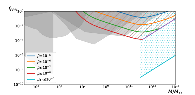
Figure 3: Constraints on the fraction of dark matter in monochromatic PBHs within the mass range $10^{2}-10^{15}M_{\odot}$ . The gray regions (adapted from fig. 10 in ref. Carr et al. (2020)) have been ruled out by current observations Oguri et al. (2018); Serpico et al. (2020); Inoue and Kusenko (2017); Carr and Silk (2018). Colored curves are possible upper bounds for $f_{PBH}$ if future observations find certain upper bounds for the average $\mu$-distortion in CMB: $\bar{\mu}\lesssim 10^{-5}$ (blue), $\bar{\mu}\lesssim 10^{-6}$ (orange), $\bar{\mu}\lesssim 10^{-7}$ (green) and $\bar{\mu}\lesssim 10^{-8}$ (red). The purple line is imposed by condition (16) that there should at least be one black holes within the smallest patch future missions can measure. The cyan line is a possible bound if future observations find $\mu\lesssim 10^{-8}$ at an angular scale $\sim 1^{\circ}$.

As for the spiky distortions in possibly rare spots on the CMB sky, by eq. (13) we have $\mu_{M}>10^{-7}$ for $M>10^{12}M_{\odot}$. Considering that signals of this kind will be measured in a patch of angular scale $\sim 1^{\circ}$, which contains $\mathcal{O}(10)$ Silk patches, a single black hole with $M>10^{12}M_{\odot}$ should give $\mu_{1^{\circ}}>10^{-8}$ in a single pixel. If there is no indication of such signals, the PBH mass function can be constrained by $n_{M}\lesssim\left[4\pi\left(10\ \text{Gpc}\right)^{2}\left(50\ \text{Mpc}\right)\right]^{-1}\sim 10^{-11}\ \text{Mpc}^{-3}$, which means there is not a single stupendously large black hole living on the CMB sky (here $10\ \text{Gpc}$ is the comoving radius of the last scattering surface). By eq. (15), we have

$$f(M>10^{12}M_{\odot})\sim 10^{-10}\frac{M}{M_{\odot}}n_{M}\ \text{Mpc}^{3}\lesssim 10^{-21}\frac{M}{M_{\odot}},$$ (20)

which is even more stringent than the bound given by $\bar{\mu}$ at $M>10^{12}M_{\odot}$. This possible bound is shown as the cyan line in fig. 3.

III Conclusions and discussion

In this paper we have studied the possible $\mu$-distortion in the CMB spectrum around supermassive PBHs and how future observations might impose constraints on the PBH density within the mass range $\mathcal{O}(10^{6}-10^{15})M_{\odot}$. Our discussion is based on the assumption that each PBH is formed with a surrounding underdense region that roughly compensates the black hole mass. This should apply to a number of mechanisms of PBH formation, including PBHs from inflationary density fluctuations, topological defects, phase transitions, etc., where the total mass excess of the perturbation (approximately) vanishes. As the underdense region expands outwards as a wave packet at the speed of sound, which we refer to as a sound shell, dissipation of the wave due to photon diffusion can inject energy into the background and thus produce $\mu$-distortion in the CMB spectrum.

If there are more than one PBH with $M\gtrsim 10^{6}M_{\odot}$ within a Silk region, which is of an angular scale of $0.2^{\circ}$, we can have an average distortion $\bar{\mu}$ in CMB. The possible non-observation of $\bar{\mu}$ in future missions beyond the $\Lambda$CDM model (which predicts $\bar{\mu}\sim 10^{-8}$) would then place constraints on these black holes. A bound of particular interest would be $f<10^{-3}$ for $10^{10}M_{\odot}\lesssim M\lesssim 10^{12}M_{\odot}$.

Even if these supermassive PBHs are rare in our universe, it is possible that we can see pointlike distortions with magnitude $\mu_{M}\gtrsim 10^{-7}$ on some Silk patches in CMB, as long as the black holes have initial mass $M\gtrsim 10^{12}M_{\odot}$. Considering that the resolution of future missions could reach $\delta\theta\sim 1^{\circ}$, such a signal in a pixel would be $\mu_{1^{\circ}}\gtrsim 10^{-8}$. The non-observation would imply that these stupendously large PBHs can only constitute a tiny part of the dark matter, with a fraction $f<10^{-9}$ for $M\sim 10^{12}M_{\odot}$.

Our main results are shown in fig. 3. If future observations do not see $\mu$-distortion with $\mu\gtrsim 10^{-8}$, the shaded regions in the figure, including that with (brown) tilted lines and that with (cyan) dots, should all be excluded. An exciting possibility is that we do see local distortions in CMB, which would be a hint of the existence of stupendously large PBHs, and we will be able to estimate their population by eq. (13).

Two assumptions that lead to our results are (a) the black hole is formed at a time $t_{M}\sim M$; (b) the underdense region is of a scale $D\sim M$ at $t_{M}$. While these are plausible assumptions, the exact values of $t_{M}$ and $D$ are model dependent, and can even vary with different PBH masses in a given model. Typically, we would expect $t_{M}=\mathcal{O}(1-10)M$ and $D=\mathcal{O}(1-10)M$. In this case, the bounds shown in fig. 3 should be adjusted accordingly.

An important aspect we did not consider is the mass accretion of PBHs. It is possible that supermassive PBHs did not acquire much accretion, which naturally explains the proportionality between the masses of supermassive black holes and those of galaxies Carr and Silk (2018). But this seems unlikely. Although the increase in mass is insignificant during the radiation era, a large amount of gas (including dark matter), be it galactic or intergalactic, is expected to fall into the black hole after the dust-radiation equality. Many works have been done constraining the PBH density with mass accretion of the Bondi-type Carr (1981); Ricotti et al. (2008); Ricotti (2007); Ali-Haïmoud and Kamionkowski (2017). The accretion rate, however, is highly model dependent. It is also known (and particularly pointed out in ref. Carr et al. (2021)) that the Bondi process is only valid for black holes with $M\lesssim 10^{4}M_{\odot}$, and the physics of mass accretion for stupendously large PBHs is still unclear. When taking into account mass accretion, a naive expectation is that the bounds shown in fig. 3 should be deformed and shifted toward the right.

Lastly, although the focus of the present work is on the $\mu$-distortion generated by the Silk damping of the sound shell, it should be mentioned that the shell itself can be a source of temperature perturbations in CMB. At the time of recombination ($t\sim 10^{13}\ \text{s}$), the shell’s radius ($\sim$ sound horizon) is of an angular size $\sim 1^{\circ}$ on the CMB sky, and its thickness is the Silk damping scale $\sim 0.2^{\circ}$ ($S\sim\Lambda$), which is comparable to the thickness of the last scattering surface. Therefore, the underdensity and overdensity on the shell (fig. 2) can induce a ring-like feature in CMB (the ring’s radius depends on the black hole’s position relative to the last scattering surface). Since temperature in the radiation era is given by $T\propto\rho^{1/4}$, where $\rho$ is the radiation density, then by eq. (47) in the appendix, the temperature perturbation can be estimated as

$$\left|\frac{\delta T}{T}\right|\approx\frac{1}{4}\delta_{am}\sim 10^{-26}\left(\frac{M}{M_{\odot}}\right)^{3/2}.$$ (21)

For a black hole as massive as $10^{14}M_{\odot}$, this gives $\sim 10^{-5}$, comparable to the observed rms CMB perturbations. Hence PBHs with larger initial masses should be rare on the last scattering surface, which means these PBHs are constrained by the cyan bound in fig. 3.

Appendix: Sound shell in a viscous radiation fluid

In this appendix we study the evolution of a spherical sound wave packet expanding in a radiation-dominated universe, and how its energy gets dissipated by viscosity.

(a) Minkowski, without viscosity

We first consider the sound wave equations for a perfect radiation fluid in Minkowski spacetime. Let $\rho(x^{i},\tau)$ be the energy density of the fluid, $\delta=\rho/\rho_{r}-1$ be the small density contrast (where $\rho_{r}$ is the unperturbed background density), and $u^{i}$ be the fluid velocity. The energy-momentum tensor of the fluid is

$$T^{00} =\rho_{r}(1+\delta)+\frac{4}{3}\rho_{r}u^{2},$$ (22)

$$T^{i0} =\frac{4}{3}\rho_{r}(1+\delta)u^{i},$$ (23)

$$T^{ij} =\frac{1}{3}\delta^{ij}\rho_{r}(1+\delta)+\frac{4}{3}\rho_{r}(1+\delta)u^{i}u^{j}.$$ (24)

where $u^{2}=|u^{i}u_{i}|$, and we have taken into account that the radiation pressure is $p=\rho/3$. The sound wave equations can then be found by the lineraized energy-momentum conservation, $\partial_{\mu}T^{\mu\nu}=0$:

$$3\dot{\delta}+4\partial_{i}u^{i} =0,$$ (25)

$$4\dot{u}^{i}+\partial_{i}\delta =0,$$ (26)

where $\dot{}\equiv\partial/\partial\tau$. Now let $u^{i}\equiv\partial_{i}\phi$, where $\phi$ is known as the velocity potential. Then by the second equation, we have $\delta=-4\dot{\phi}$, and the two equations can be combined into

$$\ddot{\phi}-\frac{1}{3}\nabla^{2}\phi=0,$$ (27)

which describes a wave propagating at the speed of sound $c_{s}=1/\sqrt{3}$. For a spherical wave, this equation has a general solution, $\phi=f(r-c_{s}\tau)/r$. Furthermore, since in this work we are interested in a spherical sound shell, we will approximate the wave by writing its velocity potential in a Gaussian form:

$$\phi=K\frac{d^{2}}{r}e^{-\frac{(r-r_{s})^{2}}{2d^{2}}},$$ (28)

where $d$ is the shell’s thickness, $r_{s}\equiv c_{s}\tau$ is the shell’s radius, and $K$ is a dimensionless factor. We will also assume the shell’s thickness is negligible compared to its radius, i.e., $r_{s}\gg d$. Then the density contrast and radial fluid velocity are found to be

$$\delta=-4c_{s}K\left(1-\frac{r_{s}}{r}\right)e^{-\frac{(r-r_{s})^{2}}{2d^{2}}},$$ (29)

$$u=-K\left(1+\frac{d^{2}}{r^{2}}-\frac{r_{s}}{r}\right)e^{-\frac{(r-r_{s})^{2}}{2d^{2}}}\approx-K\left(1-\frac{r_{s}}{r}\right)e^{-\frac{(r-r_{s})^{2}}{2d^{2}}}=\delta/4c_{s}.$$ (30)

We can see that $\delta>0$ for $r<r_{s}$ and $\delta<0$ for $r>r_{s}$, which means the shell consists of an underdensity and an overdensity. This is a typical feature of a spherical sound wave packet Landau and Lifshitz (2013). The amplitude of $\delta$ can be estimated as the value of $|\delta|$ at $r=r_{s}+d$, which gives

$$\delta_{am}\sim K\frac{d}{r_{s}}.$$ (31)

The energy density of the fluid is

$$T^{00}=\rho_{r}+\rho_{r}\delta+\frac{4}{3}\rho_{r}u^{2},$$ (32)

where the three terms are respectively the densities of the background, the deficit and the sound wave energy. Therefore, the energy deficit and the sound wave energy of the shell are given by

$$E_{-}=4\pi\rho_{r}\int\delta r^{2}dr\approx-73K\rho_{r}d^{3},$$ (33)

$$E_{s}=4\pi\rho_{r}\int\frac{4}{3}u^{2}r^{2}dr\approx 21K\rho_{r}d^{3},$$ (34)

both of which are constant over time.

(b) Minkowski, with viscosity

In the presence of photon diffusion, the energy-momentum tensor of the fluid acquires an extra term $\Delta T_{\mu\nu}$ that acts effectively as viscosity Weinberg (1971, 2008); Pajer and Zaldarriaga (2013). For an irrotational flow its divergence is given by

$$\partial_{\nu}\Delta T^{0\nu} =0,$$ (35)

$$\partial_{\nu}\Delta T^{i\nu} =-\frac{4}{3}\eta\nabla^{2}u^{i},$$ (36)

where the viscous coefficient $\eta$ is

$$\eta=\frac{16}{45}\rho_{r}\tau_{\gamma}.$$ (37)

Here, $\tau_{\gamma}=(\sigma_{T}n_{e})^{-1}$ is the photon’s mean free path, where $\sigma_{T}$ is the Thomson cross-section and $n_{e}$ is the electron density. With this extra term, eq. (26) becomes

$$4\dot{u}^{i}+\partial_{i}\delta-\frac{4\eta}{\rho_{r}}\partial^{2}u^{i}=0,$$ (38)

while eq. (25) remains unchanged. Then the wave equation (27) becomes

$$\ddot{\phi}-\frac{1}{3}\nabla^{2}\phi-\frac{\eta}{\rho_{r}}\nabla^{2}\dot{\phi}=0.$$ (39)

In the limit of small viscosity, this can be solved in the Fourier representation, with the result

$$\phi=K\left(\frac{d}{s}\right)\frac{d^{2}}{r}e^{-\frac{(r-r_{s})^{2}}{2s^{2}}},$$ (40)

where

$$s=\sqrt{d^{2}+\lambda^{2}}$$ (41)

with $\lambda\equiv\left(\eta t/\rho_{r}\right)^{1/2}$. By the definition of $\eta$, $\lambda\sim\left(\tau_{\gamma}t\right)^{1/2}$, which is the photon diffusion scale. Comparing this solution with eq. (28), we can see that the shell’s thickness increases with time due to the viscosity, while the amplitude of the velocity potential gets damped by $d/s$.

The fluid velocity $u=\partial_{r}\phi$ and density contrast $\delta=-4\dot{\phi}$ are then given by

$$u\approx\frac{\delta}{4c_{s}}\approx-K\left(\frac{d}{s}\right)^{3}\left(1-\frac{r_{s}}{r}\right)e^{-\frac{(r-r_{s})^{2}}{2s^{2}}}.$$ (42)

As before, the amplitude of $\delta$ can be estimated as the value of $|\delta|$ at $r=r_{s}+s$, which is

$$\delta_{am}\sim K\left(\frac{d}{s}\right)^{2}\frac{d}{r_{s}}.$$ (43)

The energy deficit and sound wave energy of the shell now become

$$E_{-}\approx-73K\rho_{r}d^{3}.$$ (44)

$$E_{s}\approx 21K\left(\frac{d}{s}\right)^{3}\rho_{r}d^{3}.$$ (45)

We can see $E_{s}$ gets damped by $(d/s)^{3}$ due to the viscosity, whereas $E_{-}$ remains constant over time.

(c) Flat FRW, with viscosity

Now if we take into account cosmic expansion, the spatial coordinate $r$ becomes the comoving radius, and time $\tau$ is understood as the conformal time, i.e., $a\text{d}\tau=\text{d}t$, where $t$ is the physical time and $a$ is the scale factor. In a flat, radiation-dominated universe, we have $a(\tau)=a_{m}\tau$ and $t=a_{m}\tau^{2}/2$, where $a_{m}$ is an integration constant Mukhanov (2005). Then eq. (42) becomes

$$u\approx\frac{\delta}{4c_{s}}\approx-K\left(\frac{D}{S}\right)^{3}\left(1-\frac{R_{s}}{R}\right)e^{-\frac{(R-R_{s})^{2}}{2S^{2}}}$$ (46)

where $R$ is the physical spatial coordinate, $R_{s}=a(\tau)c_{s}\tau=2c_{s}t$ and $S=as$ are respectively the physical radius and thickness of the sound shell, and $D=ad$. The amplitude of $\delta$ can be estimated as

$$\delta_{am}\sim K\left(\frac{D}{S}\right)^{2}\frac{D}{R_{s}}.$$ (47)

The sound wave energy of the shell now becomes

$$E_{s}(t)\approx 21K\left(\frac{D}{S}\right)^{3}\rho_{r}D^{3}.$$ (48)

Without the damping factor $(D/S)^{3}$, we have $D=S,$ then since $\rho_{r}\propto a^{-4}$ and $D^{3}\propto a^{3}$, $E_{s}$ gets redshifted over time.

In our scenario, the sound shell starts as an underdense region compensating the black hole mass $M$ when the black hole is formed. By the results in eqs. (33) and (34), this means $E_{s}(t_{M})\sim M$, where $t_{M}$ is the black hole formation time. For simplicity, we assume $t_{M}\sim D(t_{M})\sim M$, which then gives

$$E_{s}(t)\sim\left(\frac{D}{S}\right)^{3}\frac{M^{2}}{D}.$$ (49)

Here, $D\sim\sqrt{Mt}$ and $S=\sqrt{D^{2}+\Lambda^{2}}$, with $\Lambda=a\lambda$ being the physical scale of photon diffusion.

It can also be shown that the amplitude of the density contrast $\delta$ can be rewritten as

$$\delta_{am}\sim\left(\frac{D}{S}\right)^{2}\frac{M}{D},$$ (50)

which can be used to estimate the temperature perturbations on the shell.

References

- Carr et al. (2020) B. Carr, K. Kohri, Y. Sendouda, and J. Yokoyama (2020), eprint 2002.12778.
- Bird et al. (2016) S. Bird, I. Cholis, J. B. Muñoz, Y. Ali-Haïmoud, M. Kamionkowski, E. D. Kovetz, A. Raccanelli, and A. G. Riess, Phys. Rev. Lett. 116, 201301 (2016), eprint 1603.00464.
- Sasaki et al. (2016) M. Sasaki, T. Suyama, T. Tanaka, and S. Yokoyama, Phys. Rev. Lett. 117, 061101 (2016), eprint 1603.08338.
- Clesse and García-Bellido (2017) S. Clesse and J. García-Bellido, Phys. Dark Univ. 15, 142 (2017), eprint 1603.05234.
- Abbott et al. (2019) B. P. Abbott et al. (LIGO Scientific, Virgo), Phys. Rev. X 9, 031040 (2019), eprint 1811.12907.
- Abbott et al. (2020a) R. Abbott et al. (LIGO Scientific, Virgo) (2020a), eprint 2010.14527.
- Abbott et al. (2020b) R. Abbott et al. (LIGO Scientific, Virgo), Phys. Rev. Lett. 125, 101102 (2020b), eprint 2009.01075.
- Woosley (2017) S. E. Woosley, Astrophys. J. 836, 244 (2017), eprint 1608.08939.
- Belczynski et al. (2016) K. Belczynski et al., Astron. Astrophys. 594, A97 (2016), eprint 1607.03116.
- Spera and Mapelli (2017) M. Spera and M. Mapelli, Mon. Not. Roy. Astron. Soc. 470, 4739 (2017), eprint 1706.06109.
- Giacobbo et al. (2018) N. Giacobbo, M. Mapelli, and M. Spera, Mon. Not. Roy. Astron. Soc. 474, 2959 (2018), eprint 1711.03556.
- Lynden-Bell (1969) D. Lynden-Bell, Nature 223, 690 (1969).
- Kormendy and Richstone (1995) J. Kormendy and D. Richstone, Ann. Rev. Astron. Astrophys. 33, 581 (1995).
- Wang et al. (2021) F. Wang, J. Yang, X. Fan, J. F. Hennawi, A. J. Barth, E. Banados, F. Bian, K. Boutsia, T. Connor, F. B. Davies, et al., The Astrophysical Journal Letters 907, L1 (2021).
- Haiman (2004) Z. Haiman, Astrophys. J. 613, 36 (2004), eprint astro-ph/0404196.
- Rubin et al. (2001) S. G. Rubin, A. S. Sakharov, and M. Yu. Khlopov, J. Exp. Theor. Phys. 91, 921 (2001), [J. Exp. Theor. Phys.92,921(2001)], eprint hep-ph/0106187.
- Bean and Magueijo (2002) R. Bean and J. Magueijo, Phys. Rev. D66, 063505 (2002), eprint astro-ph/0204486.
- Duechting (2004) N. Duechting, Phys. Rev. D70, 064015 (2004), eprint astro-ph/0406260.
- Carr and Silk (2018) B. Carr and J. Silk, Mon. Not. Roy. Astron. Soc. 478, 3756 (2018), eprint 1801.00672.
- Carr and Kuhnel (2020) B. Carr and F. Kuhnel, Ann. Rev. Nucl. Part. Sci. 70, 355 (2020), eprint 2006.02838.
- Hawking (1989) S. W. Hawking, Phys. Lett. B 231, 237 (1989).
- Polnarev and Zembowicz (1991) A. Polnarev and R. Zembowicz, Phys. Rev. D 43, 1106 (1991).
- Garriga and Vilenkin (1993) J. Garriga and A. Vilenkin, Phys. Rev. D 47, 3265 (1993), eprint hep-ph/9208212.
- Caldwell and Casper (1996) R. R. Caldwell and P. Casper, Phys. Rev. D 53, 3002 (1996), eprint gr-qc/9509012.
- Hawking et al. (1982) S. W. Hawking, I. G. Moss, and J. M. Stewart, Phys. Rev. D 26, 2681 (1982).
- Rubin et al. (2000) S. G. Rubin, M. Y. Khlopov, and A. S. Sakharov, Grav. Cosmol. 6, 51 (2000), eprint hep-ph/0005271.
- Khlopov et al. (2005) M. Y. Khlopov, S. G. Rubin, and A. S. Sakharov, Astropart. Phys. 23, 265 (2005), eprint astro-ph/0401532.
- Garriga et al. (2016) J. Garriga, A. Vilenkin, and J. Zhang, JCAP 02, 064 (2016), eprint 1512.01819.
- Carr and Lidsey (1993) B. J. Carr and J. E. Lidsey, Phys. Rev. D 48, 543 (1993).
- Kohri et al. (2014) K. Kohri, T. Nakama, and T. Suyama, Phys. Rev. D 90, 083514 (2014), eprint 1405.5999.
- Nakama et al. (2016) T. Nakama, T. Suyama, and J. Yokoyama, Phys. Rev. D 94, 103522 (2016), eprint 1609.02245.
- Nakama et al. (2018) T. Nakama, B. Carr, and J. Silk, Phys. Rev. D 97, 043525 (2018), eprint 1710.06945.
- Kawasaki and Murai (2019) M. Kawasaki and K. Murai, Phys. Rev. D 100, 103521 (2019), eprint 1907.02273.
- Atal et al. (2021) V. Atal, A. Sanglas, and N. Triantafyllou, JCAP 06, 022 (2021), eprint 2012.14721.
- Carr et al. (2021) B. Carr, F. Kuhnel, and L. Visinelli, Mon. Not. Roy. Astron. Soc. 501, 2029 (2021), eprint 2008.08077.
- Ivanov et al. (1994) P. Ivanov, P. Naselsky, and I. Novikov, Phys. Rev. D 50, 7173 (1994).
- Garcia-Bellido et al. (1996) J. Garcia-Bellido, A. D. Linde, and D. Wands, Phys. Rev. D 54, 6040 (1996), eprint astro-ph/9605094.
- Kawasaki et al. (1998) M. Kawasaki, N. Sugiyama, and T. Yanagida, Phys. Rev. D 57, 6050 (1998), eprint hep-ph/9710259.
- Yokoyama (1998) J. Yokoyama, Phys. Rev. D 58, 083510 (1998), eprint astro-ph/9802357.
- Garcia-Bellido and Ruiz Morales (2017) J. Garcia-Bellido and E. Ruiz Morales, Phys. Dark Univ. 18, 47 (2017), eprint 1702.03901.
- Hertzberg and Yamada (2018) M. P. Hertzberg and M. Yamada, Phys. Rev. D 97, 083509 (2018), eprint 1712.09750.
- Harada and Carr (2005) T. Harada and B. J. Carr, Phys. Rev. D 71, 104009 (2005), eprint astro-ph/0412134.
- Carr and Harada (2015) B. J. Carr and T. Harada, Phys. Rev. D 91, 084048 (2015), eprint 1405.3624.
- Harada et al. (2015) T. Harada, C.-M. Yoo, T. Nakama, and Y. Koga, Phys. Rev. D 91, 084057 (2015), eprint 1503.03934.
- Musco (2019) I. Musco, Phys. Rev. D 100, 123524 (2019), eprint 1809.02127.
- Germani and Musco (2019) C. Germani and I. Musco, Phys. Rev. Lett. 122, 141302 (2019), eprint 1805.04087.
- Kehagias et al. (2019) A. Kehagias, I. Musco, and A. Riotto, JCAP 12, 029 (2019), eprint 1906.07135.
- Deng et al. (2017) H. Deng, J. Garriga, and A. Vilenkin, JCAP 04, 050 (2017), eprint 1612.03753.
- Deng and Vilenkin (2017) H. Deng and A. Vilenkin, JCAP 1712, 044 (2017), eprint 1710.02865.
- Deng (2020a) H. Deng, JCAP 09, 023 (2020a), eprint 2006.11907.
- Deng et al. (2018) H. Deng, A. Vilenkin, and M. Yamada, JCAP 07, 059 (2018), eprint 1804.10059.
- Deng (2020b) H. Deng, JCAP 05, 037 (2020b), eprint 2003.02485.
- Landau and Lifshitz (2013) L. D. Landau and E. M. Lifshitz, Fluid Mechanics (Elsevier Science, 2013), 2nd ed.
- Weinberg (1971) S. Weinberg, Astrophys. J. 168, 175 (1971).
- Weinberg (2008) S. Weinberg, Cosmology (Oxford university press, 2008).
- Pajer and Zaldarriaga (2013) E. Pajer and M. Zaldarriaga, JCAP 02, 036 (2013), eprint 1206.4479.
- Khatri and Sunyaev (2015) R. Khatri and R. Sunyaev, JCAP 09, 026 (2015), eprint 1507.05615.
- Sunyaev and Zeldovich (1970) R. Sunyaev and Y. B. Zeldovich, Astrophysics and Space Science 7, 20 (1970).
- Daly (1991) R. Daly, The Astrophysical Journal 371, 14 (1991).
- Barrow and Coles (1991) J. D. Barrow and P. Coles, Monthly Notices of the Royal Astronomical Society 248, 52 (1991).
- Hu and Silk (1993) W. Hu and J. Silk, Phys. Rev. D 48, 485 (1993).
- Silk (1968) J. Silk, Astrophys. J. 151, 459 (1968).
- Fixsen et al. (1996) D. J. Fixsen, E. S. Cheng, J. M. Gales, J. C. Mather, R. A. Shafer, and E. L. Wright, Astrophys. J. 473, 576 (1996), eprint astro-ph/9605054.
- Kogut et al. (2019) A. Kogut, M. H. Abitbol, J. Chluba, J. Delabrouille, D. Fixsen, J. C. Hill, S. P. Patil, and A. Rotti (2019), eprint 1907.13195.
- Chluba et al. (2019) J. Chluba et al. (2019), eprint 1909.01593.
- Cabass et al. (2016) G. Cabass, A. Melchiorri, and E. Pajer, Phys. Rev. D 93, 083515 (2016), eprint 1602.05578.
- Chluba (2016) J. Chluba, Mon. Not. Roy. Astron. Soc. 460, 227 (2016), eprint 1603.02496.
- Oguri et al. (2018) M. Oguri, J. M. Diego, N. Kaiser, P. L. Kelly, and T. Broadhurst, Phys. Rev. D 97, 023518 (2018), eprint 1710.00148.
- Serpico et al. (2020) P. D. Serpico, V. Poulin, D. Inman, and K. Kohri, Phys. Rev. Res. 2, 023204 (2020), eprint 2002.10771.
- Inoue and Kusenko (2017) Y. Inoue and A. Kusenko, JCAP 10, 034 (2017), eprint 1705.00791.
- Carr (1981) B. Carr, Monthly Notices of the Royal Astronomical Society 194, 639 (1981).
- Ricotti et al. (2008) M. Ricotti, J. P. Ostriker, and K. J. Mack, Astrophys. J. 680, 829 (2008), eprint 0709.0524.
- Ricotti (2007) M. Ricotti, Astrophys. J. 662, 53 (2007), eprint 0706.0864.
- Ali-Haïmoud and Kamionkowski (2017) Y. Ali-Haïmoud and M. Kamionkowski, Phys. Rev. D 95, 043534 (2017), eprint 1612.05644.
- Mukhanov (2005) V. Mukhanov, Physical foundations of cosmology (Cambridge university press, 2005).