Escaping strict saddle points of the Moreau envelope in nonsmooth optimization

Abstract

Recent work has shown that stochastically perturbed gradient methods can efficiently escape strict saddle points of smooth functions. We extend this body of work to nonsmooth optimization, by analyzing an inexact analogue of a stochastically perturbed gradient method applied to the Moreau envelope. The main conclusion is that a variety of algorithms for nonsmooth optimization can escape strict saddle points of the Moreau envelope at a controlled rate. The main technical insight is that typical algorithms applied to the proximal subproblem yield directions that approximate the gradient of the Moreau envelope in relative terms.

1 Introduction

Though nonconvex optimization problems are NP hard in general, simple nonconvex optimization techniques, e.g., gradient descent, are broadly used and often highly successful in high-dimensional statistical estimation and machine learning problems. A common explanation for their success is that smooth nonconvex functions $g\colon\mathbb{R}^{d}\rightarrow\mathbb{R}$ found in machine learning have amenable geometry: all local minima are (nearly) global minima and all saddle points are strict (i.e., have a direction of negative curvature). This explanation is well grounded: several important estimation and learning problems have amenable geometry [17, 43, 3, 16, 44, 47], and simple randomly initialized iterative methods, such as gradient descent, asymptotically avoid strict saddle points [28, 27]. Moreover, “randomly perturbed” variants [24] “efficiently” converge to $(\varepsilon_{1},\varepsilon_{2})$-approximate second-order critical points, meaning those satisfying

$$\|\nabla g(x)\|\leq\varepsilon_{1}\qquad\text{and}\qquad\lambda_{\min}(\nabla^{2}g(x))\geq-\varepsilon_{2}.$$ (1.1)

Recent work furthermore extends these results to $C^{2}$ smooth manifold constrained optimization [6, 45, 15]. Other extensions to nonsmooth convex constraint sets have proposed second-order methods for avoiding saddle points, but such methods must at every step minimize a nonconvex quadratic over a convex set (an NP hard problem in general) [18, 31, 35].

While impressive, the aforementioned works crucially rely on smoothness of objective functions or constraint sets. This is not an artifact of their proof techniques: there are simple $C^{1}$ functions for which randomly initialized gradient descent with constant probability converges to points that admit directions of second order descent [11, Figure 1]. Despite this example, recent work [11] shows that randomly initialized proximal methods avoid certain “active” strict saddle points of (nonsmooth) weakly convex functions. The class of weakly convex functions is broad, capturing, for example those formed by composing convex functions $h$ with smooth nonlinear maps $c$, which often appear in statistical recovery problems. They moreover show that for “generic” semialgebraic problems, every critical point is either a local minimizer or an active strict saddle. A key limitation of [11], however, is that the result is asymptotic, and in fact pure proximal methods may take exponentially many iterations to find local minimizers [13]. Motivated by [11], the recent work [21] develops efficiency estimates for certain randomly perturbed proximal methods. The work [21] has two limitations: its measure of complexity appears to be algorithmically dependent and the results do not extend to subgradient methods.

The purpose of this paper is to develop “efficient” methods for escaping saddle points of weakly convex functions. Much like [21], our approach is based on [11], but the resulting algorithms and their convergence guarantees are distinct from those in [21]. We begin with a useful observation from [11]: near active strict saddle points $\bar{x}$, a certain $C^{1}$ smoothing, called the Moreau envelope, is $C^{2}$ and has a strict saddle point at $\bar{x}$. If one could exactly execute the perturbed gradient method of [24], efficiency guarantees would then immediately follow. While this is not possible in general, it is possible to inexactly evaluate the gradient of the Moreau envelope by solving a strongly convex optimization problem. Leveraging this idea, we extend the work [24] to allow for inexact gradient evaluations, proving similar efficiency guarantees.

Setting the stage, we consider a minimization problem

$$\operatornamewithlimits{minimize}_{x\in\mathbb{R}^{d}}f(x)$$ (1.2)

where $f\colon\mathbb{R}^{d}\rightarrow\mathbb{R}\cup\{+\infty\}$ is closed and $\rho$-weakly convex, meaning the mapping $x\mapsto f(x)+\frac{\rho}{2}\|x\|^{2}$ is convex. Although such functions are nonsmooth in general, they admit a global $C^{1}$ smoothing furnished by the Moreau envelope. For all $\mu<\rho^{-1}$, the Moreau envelope and the proximal mapping are defined to be

$$f_{\mu}(x)=\min_{y\in\mathbb{R}^{d}}~{}f(y)+\frac{1}{2\mu}\|y-x\|^{2}\quad\text{and}\quad\mathrm{prox}_{\mu f}(x)=\operatornamewithlimits{argmin}_{y\in\mathbb{R}^{d}}f(y)+\frac{1}{2\mu}\|y-x\|^{2},$$ (1.3)

respectively. The minimizing properties of $f$ and $f_{\mu}$ are moreover closely aligned, for example, their first-order critical points and local/global minimizers coincide. Inspired by this relationship, this work thus seeks $(\varepsilon_{1},\varepsilon_{2})$-approximate second-order critical points $x$ of $f_{\mu}$, satisfying:

$$\|\nabla f_{\mu}(x)\|\leq\varepsilon_{1}\qquad\text{and}\qquad\lambda_{\min}(\nabla^{2}f_{\mu}(x))\geq-\varepsilon_{2}.$$ (1.4)

An immediate difficulty is that $f_{\mu}$ is not $C^{2}$ in general. Indeed, the seminal work [29] shows $f_{\mu}$ is $C^{2}$-smooth globally, if and only if, $f$ is $C^{2}$-smooth globally. Therefore assuming that $f_{\mu}$ is $C^{2}$ globally is meaningless for nonsmooth optimization. Nevertheless, known results in [12] imply that for “generic” semialgebraic functions, $f_{\mu}$ is locally $C^{2}$ near $x$ whenever $\|\nabla f_{\mu}(x)\|$ is sufficiently small.

Turning to algorithm design, a natural strategy is to apply a “saddle escaping” gradient method [24] directly to $f_{\mu}$. This strategy fails in general, since it is not possible to evaluate the gradient

$$\nabla f_{\mu}(x)=\frac{1}{\mu}(x-\mathrm{prox}_{\mu f}(x))$$ (1.5)

in closed form. Somewhat expectedly, however, our first contribution is to show that one may extend the results of [24] to allow for inexact evaluations $G(x)\approx\nabla f_{\mu}(x)$ satisfying

$$\|G(x)-\nabla f_{\mu}(x)\|\leq a\|\nabla f_{\mu}(x)\|+b\qquad\text{for all }x\in\mathbb{R}^{d},$$

for appropriately small $a,b\geq 0$. The algorithm (Algorithm 1) returns a point $x$ satisfying (1.4), with $\tilde{\mathcal{O}}(\max\{\varepsilon_{1}^{-2},\varepsilon_{2}^{-4}\})$ evaluations of $G$, matching the complexity of [24].

Our second contribution constructs approximate oracles $G(x)$, tailored to common problem structures. Each oracle satisfies

$$G(x)=\mu^{-1}\left(x-\textsc{ProxOracle}_{\mu f}(x)\right),$$

where $\textsc{ProxOracle}_{\mu f}$ is an approximate minimizer of the strongly convex subproblem defining $\mathrm{prox}_{\mu f}(x)$. Since the subproblem is strongly convex, we construct $\textsc{ProxOracle}_{\mu f}$ from $K$ iterations of off-the-shelf first-order methods for convex optimization. We focus in particular on the class of model-based methods [10]. Starting from initial point $x_{0}=x$, these methods attempt to minimize $f(y)+\frac{1}{2\mu}\|y-x\|^{2}$ by iterating

$$x_{k+1}=\operatornamewithlimits{argmin}_{y\in\mathbb{R}^{d}}\left\{f_{x_{k}}(y)+\frac{1}{2\mu}\|y-x\|^{2}+\frac{\theta_{k}}{2}\|y-x_{k}\|^{2}\right\},$$ (1.6)

where $\theta_{k}>0$ is a control sequence and for all $z\in\mathbb{R}^{d}$, the function $f_{z}\colon\mathbb{R}^{d}\rightarrow\mathbb{R}\cup\{+\infty\}$ is a local weakly convex model of $f$. In Table 1, we show three models, adapted to possible decompositions of $f$. In Table 2, we show how the model function $f_{z}$ influences the total complexity $\tilde{\mathcal{O}}(K\times\max\{\varepsilon_{1}^{-2},\varepsilon_{2}^{-4}\})$ of finding a second order stationary point of $f_{\mu}$ (1.4). In short, prox-gradient and prox-linear methods require $\tilde{\mathcal{O}}(\max\{\varepsilon_{1}^{-2},\varepsilon_{2}^{-4}\})$ iterations of (1.6), while prox-subgradient methods require $\tilde{\mathcal{O}}(d\max\{\varepsilon_{1}^{-6}\varepsilon_{2}^{-6},\varepsilon_{2}^{-18}\})$. The efficiency of the prox-gradient method directly matches the analogous guarantees for the perturbed gradient method in the smooth setting [24]. The convergence guarantee of the prox-subgradient method has no direct analogue in the literature. Extensions for stochastic variants of these algorithms follow trivially, when the proximal subproblem (1.6) can be approximately solved with high probability (e.g. using [19, 20, 26, 39]). The rates for the prox-gradient and prox-linear method are analogous to those in [21], which uses an algorithm-dependent measure of stationarity. Although the algorithms and the results in our paper and in [21] are mostly of theoretical interest, they do suggest that efficiently escaping from saddle points is possible in nonsmooth optimization.

Algorithm	Objective	Model function $f_{z}(y)$
Prox-Subgradient [10]	$\displaystyle l(y)+r(y)$	$\displaystyle l(z)+\langle v_{z},y-z\rangle+r(y)$
Prox-gradient	$\displaystyle F(y)+r(y)$	$\displaystyle F(z)+\langle\nabla F(y),y-z\rangle+r(y)$
Prox-linear [14]	$\displaystyle h(c(x))+r(x)$	$\displaystyle h(c(x)+\nabla c(x)(y-x))+r(y)$

Table 1: The three algorithms with the update (1.6); we assume $h$ is convex and Lipschitz, $r$ is weakly convex and possibly infinite valued, both $F$ and $c$ are smooth, and $l$ is Lipschitz and weakly convex on $\mathrm{dom}\;r$ with $v_{z}\in\partial l(z)$.

Algorithm to Evaluate $g(x)$	Overall Algorithm Complexity
Prox-Subgradient [10]	$\displaystyle\tilde{\mathcal{O}}(d\max\{\varepsilon_{1}^{-6}\varepsilon_{2}^{-6},\varepsilon_{2}^{-18}\})$
Prox-gradient	$\displaystyle\tilde{\mathcal{O}}(\max\{\varepsilon_{1}^{-2},\varepsilon_{2}^{-4}\})$
Prox-linear [14]	$\displaystyle\tilde{\mathcal{O}}(\max\{\varepsilon_{1}^{-2},\varepsilon_{2}^{-4}\})$

Table 2: The overall complexity of the proposed algorithm $\tilde{\mathcal{O}}(K\times\max\{\varepsilon_{1}^{-2},\varepsilon_{2}^{-4}\})$, where $K$ is the number of steps of (1.6) required to evaluate $g(x)$. The rate for Prox-subgradient holds in the regime $\varepsilon_{1}=\mathcal{O}(\varepsilon_{2})$.

Related work. We highlight several approaches for finding second-order critical points. Asymptotic guarantees have been developed in deterministic [28, 27, 11] and stochastic settings [38]. Other approaches explicitly leverage second order information about the objective function, such as full Hessian or Hessian vector products computations [34, 8, 1, 5, 2, 41, 42, 37, 7]. Several methods exploit only first-order information combined with random perturbations [15, 24, 9, 25, 23]. The work [23] also studies saddle avoiding methods with inexact gradient oracles $G$; a key difference: the oracle of [23] is the gradient of a smooth function $G=\nabla g$. Several existing works have developed methods that find second-order stationary points of manifold [6, 45], convex [31, 35, 30, 48], and low-rank matrix constrained problems [49, 36].

Road map. In Section 2 we introduce the preliminaries. Section 3 presents a result for finding second-order stationary points with inexact gradient evaluations. Section 4 develops several oracle mappings that approximately evaluate the gradient of the Moreau Envelope and derives the complexity estimates of Table 2.

2 Preliminaries

This section summarizes the notation that we use throughout the paper. We endow $\mathbb{R}^{d}$ with the standard inner product $\langle x,y\rangle:=x^{\top}y$ and the induced norm $\|x\|_{2}:=\sqrt{\langle x,x\rangle}$. The closed unit ball in $\mathbb{R}^{d}$ will be denoted by $\mathbb{B}^{d}:=\{x\in\mathbb{R}^{d}\mid\|x\|\leq 1\}$, while a closed ball of radius $r>0$ around a point $x$ will be written as $\mathbb{B}_{r}^{d}(x)$. When the dimension is clear from the context we write $\mathbb{B}$. Given a function $\varphi\colon\mathbb{R}^{d}\to\mathbb{R}\cup\{\infty\}$, the domain and the epigraphs of $\varphi$ are given by $\mathrm{dom}\;\varphi=\{x\in\mathbb{R}^{d}\mid\varphi(x)<\infty\}\text{ and }\mathrm{epi}\;\varphi=\{(x,r)\mid\varphi(x)\leq r\}.$ A function $\varphi$ is called closed if $\mathrm{epi}\;\varphi$ is a closed set. The distance of a point $x\in\mathbb{R}^{d}$ to a set $\mathcal{M}\subseteq\mathbb{R}^{d}$ is denoted by ${\rm dist}(x,\mathcal{M})=\inf_{y\in\mathcal{M}}\|x-y\|.$ The symbol $\|A\|$ denotes the operator norm of a matrix $A$, while the maximal and minimal eigenvalues of a symmetric matrix $A$ will be denoted by $\lambda_{\max}(A)$ and $\lambda_{\min}(A)$, respectively. For any bounded measurable set $Q\subset\mathbb{R}^{d}$, we let $\mathrm{Unif}(Q)$ be the uniform distribution over $Q$.

We will require some basic constructions from Variational Analysis as described for example in the monographs [40, 32, 4]. Consider a closed function $f\colon\mathbb{R}^{d}\to\mathbb{R}\cup\{\infty\}$ and a point $x$, with $f(x)$ finite. The subdifferential of $f$ at $x$, denoted by $\partial f(x)$, is the set of all vectors $v\in\mathbb{R}^{d}$ satisfying

$$f(y)\geq f(x)+\langle v,y-x\rangle+o(\|y-x\|_{2})\quad\textrm{as }y\to x.$$ (2.1)

We set $\partial f(x)=\emptyset$ when $x\notin\mathrm{dom}\;f$. When $f$ is $C^{1}$ at $x\in\mathbb{R}^{d}$, the subdifferential $\partial f(x)$ consists of the gradient $\{\nabla f(x)\}$. When $f$ is convex, it reduces to the subdifferential in the sense of convex analysis. In this work, we will primarily be interested in the class of $\rho$-weakly convex functions, meaning those for which $x\mapsto f(x)+\frac{\rho}{2}\|x\|^{2}$ is convex. For $\rho$-weakly convex functions the subdifferential satisfies:

$$f(y)\geq f(x)+\langle v,y-x\rangle-\frac{\rho}{2}\|y-x\|^{2},\qquad\text{for all }x,y\in\mathbb{R}^{d},v\in\partial f(x).$$

Finally, we mention that a point $x$ is a first-order critical point of $f$ whenever the inclusion $0\in\partial f(x)$ holds.

3 Escaping saddle points with inexact gradients

In this section, we analyze an inexact gradient method on smooth functions, focusing on convergence to second-order stationary points. The consequences for nonsmooth optimization, which will follow from a smoothing technique, will be explored in Section 3.

We begin with the following standard assumption, which asserts that the function $f$ in question has a globally Lipchitz continuous gradient.

Assumption A (Globally Lipschitz gradient).

Fix a function $g\colon\mathbb{R}^{d}\to\mathbb{R}$ that is bounded from below and whose gradient is globally Lipschitz continuous with constant $L_{1}$, meaning

$$\|\nabla g(x)-\nabla g(y)\|\leq L_{1}\|x-y\|\qquad\text{for all }x,y\in\mathbb{R}^{d}.$$

The next assumption is more subtle: it requires the Hessian $\nabla^{2}g$ to be Lipschitz continuous on a neighborhood of any point where the gradient is sufficiently small. When we discuss consequences for nonsmooth optimization in the later sections, the fact that $f$ is assumed to be $C^{2}$-smooth only locally will be crucial to our analysis.

Assumption B (Locally Lipschitz Hessian).

Fix a function $g\colon\mathbb{R}^{d}\to\mathbb{R}$ and assume that there exist positive constants $\alpha,\beta,L_{2}$ satisfying the following: For any point $\bar{x}$ with $\|\nabla g(\bar{x})\|\leq\alpha$, the function $g$ is $C^{2}$-smooth on $\mathbb{B}_{\beta}(\bar{x})$ and satisfies the Lipschitz condition:

$$\|\nabla^{2}g(x)-\nabla^{2}g(y)\|\leq L_{2}\|x-y\|\qquad\text{for all }x,y\in B_{\beta}(\bar{x}).$$

We aim to analyze an inexact gradient method for minimizing the function $f$ under Assumptions A and B. The type of inexactness we allow is summarized by the following oracle model.

Definition 3.1 (Inexact oracle).

A map $G\colon\mathbb{R}^{d}\rightarrow\mathbb{R}^{d}$ is an $(a,b)$-inexact gradient oracle for $f$ if it satisfies

$$\left\|\nabla g(x)-G(x)\right\|\leq a\cdot\left\|\nabla g(x)\right\|+b\qquad\forall x\in\mathbb{R}^{d}.$$ (3.1)

Turning to algorithm design, the method we introduce (Algorithm 1) directly extends the perturbed gradient method introduced in [24] to inexact gradient oracles in the sense of Definition 3.1. The convergence guarantees for the algorithm will be based on the following explicit setting of parameters. Fix target accuracies $\varepsilon_{1},\varepsilon_{2}>0$ and choose any $\Delta_{g}\geq g(x_{0})-\inf g$. We first define the auxiliary parameters:

$$\small\phi:=2^{24}\max\left\{1,5\frac{L_{2}\varepsilon_{1}}{L_{1}\varepsilon_{2}}\right\}\frac{L_{1}^{2}}{\delta}\sqrt{{d}}\left(\Delta_{g}\max\left\{\frac{L_{2}^{2}}{\varepsilon_{2}^{5}},\frac{1}{\varepsilon_{1}^{2}\varepsilon_{2}^{1}}\right\}+\frac{1}{\varepsilon_{2}^{2}}\right)\quad\text{and}\quad\gamma:=\log_{2}(\phi\log_{2}(\phi)^{8}),$$ (3.2)

and

$$F=\frac{1}{800\gamma^{3}}\frac{1-a}{(1+a)^{2}}{\frac{\varepsilon_{2}^{3}}{L_{2}^{2}}}\qquad\text{and}\qquad R=\frac{1}{4\gamma}{\frac{\varepsilon_{2}}{L_{2}}}.$$

The parameters required by the algorithm are then set as

$$\begin{split}&\eta=\frac{1-a}{(1+a)^{2}}\frac{1}{L_{1}},\quad r=\frac{\varepsilon_{2}^{2}}{400L_{2}\gamma^{3}}\min\left\{1,\frac{L_{1}\varepsilon_{2}}{5\varepsilon_{1}L_{2}}\right\},\quad M=\frac{(1+a)^{2}}{(1-a)}\frac{L_{1}}{\varepsilon_{2}}\gamma.\end{split}$$ (3.3)

The following is the main result of the section. The proof follows closely the argument in [24] and therefore appears in Appendix A.

Data: $x_{0}\in\mathbb{R}^{d}$, $T\in\mathbb{N}$, and $\eta,r,\varepsilon_{1},M>0$

Set $t_{\text{pert}}=-M$

Step $t=0,\ldots,T$:

      Set $u_{t}=0$

      If $\left\|G(x_{t})\right\|\leq\varepsilon_{1}/2$ and $t-t_{\text{pert}}\geq M$:

            Update $t_{\text{pert}}=t$

            Draw perturbation $u_{t}\sim\text{Unif}(r\mathbb{B})$

      Set $\displaystyle x_{t+1}\leftarrow x_{t}-\eta\cdot(G(x_{t})+u_{t})$.

Algorithm 1 Perturbed inexact gradient descent

Theorem 3.2 (Perturbed inexact gradient descent).

Suppose that $g\colon\mathbb{R}^{d}\rightarrow\mathbb{R}$ is a function satisfying Assumptions A and B and $G\colon\mathbb{R}^{d}\rightarrow\mathbb{R}^{d}$ is an $(a,b)$-inexact gradient oracle for $g$. Let $\delta\in(0,1)$, $\varepsilon_{1}\in(0,\alpha)$, $\varepsilon_{2}\in(0,\min\{4\gamma\beta L_{2},L_{1},L_{1}^{2}\})$, and suppose that

$$\begin{split}&a\leq\min\left\{\frac{1}{20},\frac{1}{L_{1}\eta M2^{\gamma+2}},\frac{R}{\varepsilon_{1}\eta M2^{\gamma+2}}\right\}\quad\text{and}\\ &b\leq\min\left\{{\frac{\varepsilon_{1}}{64}},\left(\frac{F}{40\eta M}\right)^{1/2},\left(\frac{L_{1}F}{M(5L_{1}+1)}\right)^{1/2},\frac{R}{M\eta 2^{(\gamma+2)}}\right\}.\end{split}$$

Then with probability at least $1-\delta$, at least one iterate generated by Algorithm 1 with parameters (LABEL:eq:para) is a $(\varepsilon_{1},\varepsilon_{2})$-second-order critical point of $g$ after

$$T=8\Delta_{g}\max\left\{2\frac{M}{F},\frac{256}{(1-a)\eta\varepsilon_{1}^{2}}\right\}+4M=\tilde{\mathcal{O}}\left(L_{1}\Delta_{g}\max\left\{\frac{L_{2}^{2}}{\varepsilon_{2}^{4}},\frac{1}{\varepsilon_{1}^{2}}\right\}\right)\quad\text{iterations.}$$ (3.4)

The necessary bounds for $a$ and $b$ can be estimated as

$$\begin{split}&a\lesssim\frac{\delta}{L_{1}^{3}\Delta_{g}}\cdot d^{-1/2}\cdot\min\left\{\frac{\varepsilon_{2}^{6}}{{L_{2}^{2}}},\varepsilon_{1}^{2}\varepsilon_{2}^{2}\right\}\cdot\min\left\{{1},\frac{L_{1}\varepsilon_{2}}{L_{2}\varepsilon_{1}}\right\}^{2}\quad\text{and}\\ &b\lesssim\frac{\delta}{L_{1}^{2}L_{2}\Delta_{g}}\cdot d^{-1/2}\cdot{\min\left\{\frac{\varepsilon_{2}^{7}}{L_{2}^{2}},\varepsilon_{1}^{2}\varepsilon_{2}^{3}\right\}}\cdot\min\left\{{1},\frac{L_{1}\varepsilon_{2}}{L_{2}\varepsilon_{1}}\right\},\end{split}$$ (3.5)

where the symbol “$\lesssim$” denotes inequality up to polylogarithmic factors. Thus, Algorithm 1 is guaranteed to find a second order stationary point efficiently, provided that the gradient oracles are highly accurate. In particular, when $a=b=0$ we recover the known rates from [24].

4 Escaping saddle points of the Moreau envelope

In this section, we apply Algorithm 1 to the Moreau Envelope (1.3) of the weakly convex optimization problem (1.2) in order to find a second order stationary point of $f_{\mu}$ (1.4). We will see that a variety of standard algorithms for nonsmooth convex optimization can be used as inexact gradient oracles for the Moreau envelope. Before developing those algorithms, we summarize our main assumptions on $f_{\mu}$, describe why approximate second order stationary points of $f_{\mu}$ are meaningful for $f$, and show that Assumption B, while not automatic for general $f_{\mu}$, holds for a large class of semialgebraic functions.

As stated in the introduction, for $\mu<\rho^{-1}$, the Moreau envelope is an everywhere $C^{1}$ smooth with Lipschitz continuous gradient. In particular,

Assumption A holds automatically for $f_{\mu}$ with $L_{1}=\max\left\{\mu^{-1},\frac{\rho}{1-\mu\rho}\right\}$.

See for example [11] for a short proof. Assumption B, however, is not automatic, so we impose the following assumption throughout.

Assumption C.

Let $f\colon\mathbb{R}^{d}\rightarrow\mathbb{R}\cup\{\infty\}$ be a closed $\rho$-weakly convex function whose Moreau envelope $f_{\mu}$ satisfies Assumption B with constants $\alpha,\beta,L_{2}$.

Turning to stationarity conditions, a natural question is whether the second order condition (1.4) is meaningful for $f$. The next proposition shows that the condition (1.4) implies the existence of an approximate quadratic minorant of $f$ with small slope and curvature at a nearby point.

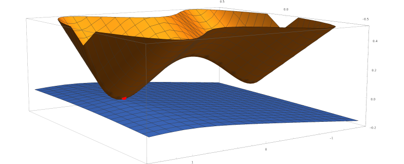
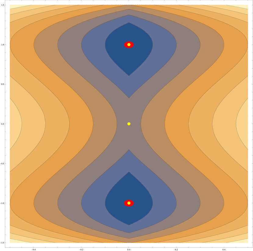
Figure 1: Critical poins of $f$ in (4.1). We use $\varepsilon_{1}=\varepsilon_{2}=0.04.$ On the left: The function, a point $(x,f(x))$ with $x$ an $(\varepsilon_{1},\varepsilon_{2})$-second-order critical point of $f_{\mu}$ and its corresponding quadratic $q(\cdot)$. On the right: The set of first-order critical points of $f$ (yellow) and the set of $(\varepsilon_{1},\varepsilon_{2})$-second-order critical points of $f_{\mu}$ (red).

We defer the proof to Appendix B.

Proposition 4.1.

Consider $f\colon\mathbb{R}^{d}\rightarrow\mathbb{R}\cup\{\infty\}$ satisfying Assumption C. Assume that $x\in\mathbb{R}^{d}$ is an $(\varepsilon_{1},\varepsilon_{2})$-second order critical point of $f_{\mu}$ with $\varepsilon_{1}\leq\min\{\alpha,\frac{\varepsilon_{2}}{2L_{2}\mu}\}$ and let $\hat{x}:=\mathrm{prox}_{\mu f}(x)$. Then there exists a quadratic function $q\colon\mathbb{R}^{d}\rightarrow\mathbb{R}$ and a neighborhood $\mathcal{U}=B_{{3\varepsilon_{2}}/{4L_{2}}}(\widehat{x})$ of $x$ for which the following hold.

1. (Nearby point) The point $\widehat{x}$ is close to $x$: $\|x-\widehat{x}\|\leq\mu\cdot\varepsilon_{1}$.

2. (Minorant) For any $y\in\mathcal{U}$, we have $q(y)\leq f(y).$

3. (Small subgradient) The quadratic has a small gradient at $\widehat{x}$:

   $$\|\nabla q(\widehat{x})\|\leq\varepsilon_{1}.$$

4. (Small negative curvature) The quadratic has small negative curvature:

   $$\nabla^{2}q(\widehat{x})\succeq-{3\varepsilon_{2}}.$$

5. (Approximate match) The quadratic almost matches the function at $\widehat{x}$:

   $$f(\widehat{x})-q(\widehat{x})\leq\frac{{\mu}}{2}\left(1+3\mu\varepsilon_{2}\right)\varepsilon_{1}^{2}.$$

In Figure 1, we illustrate the proposition with the following nonsmooth function:

$$f(x,y)=|x|+\frac{1}{4}(y^{2}-1)^{2}.$$ (4.1)

The Moreau envelope of this function has three first-order critical points: a strict saddle point $(0,0)$ and two global minima $(-1,0)$, and $(1,0)$. As shown in the right plot of Figure 1, approximate second-order critical points of $f_{\mu}$ cluster around minimizers of $f$. In addition, the left plot of Figure 1 shows the lower bounding quadratic from Proposition 4.1.

Finally, we complete this section by showing that Assumption C is reasonable: it holds for generic semialgebraic functions.

Theorem 4.2.

Let $f\colon\mathbb{R}^{d}\rightarrow\mathbb{R}\cup\{\infty\}$ be a semi-algebraic $\rho$-weakly-convex function. Then, the set of vectors $v\in{\mathcal{R}}^{d}$ for which the tilted function $g(x;v)=f(x)+\langle v,x\rangle$ satisfies Assumption C has full Lebesgue measure.

The proof appears in Appendix C, and is a small modification of the argument in [11].

4.1 Inexact Oracles for the Moreau Envelope

In this section, we develop inexact gradient oracles for $\nabla f_{\mu}=\mu^{-1}(x-\mathrm{prox}_{\mu f}(x))$. Leveraging this expression, our oracles will satisfy

$$G(x)=\mu^{-1}\left(x-\textsc{ProxOracle}_{\mu f}(x)\right),$$ (4.2)

where $\textsc{ProxOracle}_{\mu f}$ is the output of a numerical scheme that solves (1.3). To ensure $G$ meets the conditions of Definition 3.1, we require that

$$\|\textsc{ProxOracle}_{\mu f}(x)-\mathrm{prox}_{\mu f}(x)\|\leq a\cdot\|x-\mathrm{prox}_{\mu f}(x)\|+\mu\cdot b.$$

for some constants $a\in(0,1)$ and $b>0$.

Since $f$ is $\rho$-weakly convex, evaluating $\mathrm{prox}_{\mu f}(x_{k})$ amounts to minimizing the $(\mu^{-1}-\rho)$-strongly convex function $f(x)+\frac{1}{2\mu}\|x-x_{k}\|^{2}$. We now use this strong convexity to derive efficient proximal oracles via a class of algorithms called model-based methods [10], which we now briefly summarize. Given a minimization problem $\min_{x\in\mathbb{R}^{d}}g(x)$, where $g$ is strongly convex, a model-based method is an algorithm that recursively updates

$$x_{k+1}\leftarrow\operatornamewithlimits{argmin}_{x}~{}g_{x_{k}}(x)+\frac{\theta_{t}}{2}\|x-x_{k}\|^{2},$$ (4.3)

where $g_{x_{k}}\colon\mathbb{R}^{d}\rightarrow\mathbb{R}\cup\{\infty\}$ is a function that approximates $g$ near $x_{k}$. Returning to the proximal subproblem, say we wish to compute $\mathrm{prox}_{\mu f}(x_{0})$ for some given $x_{0}$. We consider an inner loop update of the form

$$x_{k+1}\leftarrow\operatornamewithlimits{argmin}_{x\in\mathbb{R}^{d}}~{}f_{x_{k}}(x)+\frac{1}{2\mu}\|x-x_{0}\|^{2}+\frac{\theta_{k}}{2}\|x-x_{k}\|^{2},$$ (4.4)

where $f_{x_{k}}\colon\mathbb{R}^{d}\rightarrow\mathbb{R}\cup\{\infty\}$ is a function that locally approximates $f$ (see Table 1 for three examples). Completing the square, this update can be equivalently written as a proximal step on $f_{x_{k}}$, where the reference point is a weighted average of $x_{0}$ and $x_{k}$ as summarized in Algorithm 2. Turning to complexity, we note that the approximation quality of a model governs the speed at which iteration (4.4) converges. In what follows, we will present two families of models with different approximation properties, namely one- and two-sided models. We will see that models with double-sided accuracy require fewer iterations to approximate $\mathrm{prox}_{\mu f}(x_{0})$.

Data: Initial point $x_{0}\in\mathbb{R}^{d}$.

Parameters: Stepsize $\theta_{k}>0$, Flag one_sided.

Output: Approximation of $\mathrm{prox}_{\mu f}(x_{0})$.

Step $k$ ($k\leq K+1$):

$\qquad x_{k+1}\leftarrow\operatornamewithlimits{argmin}_{x\in\mathbb{R}^{d}}f_{x_{k}}(x)+\frac{1+\theta_{k}\mu}{2\mu}\left\|x-\frac{\left(x_{0}+\theta_{k}\mu\cdot x_{k}\right)}{1+\theta_{k}\mu}\right\|^{2}$

If one_sided :

$\qquad\bar{x}_{K}=\frac{2}{(K+2)(K+3)-2}\sum_{k=1}^{K+1}(t+1)x_{k}$

$\qquad\textbf{return }\bar{x}_{K}$

Else:

$\qquad\textbf{return }x_{K}$

Algorithm 2 ProxOracle${}_{\mu f}^{K}$

4.1.1 One-sided models

We start by studying models that globally lower bound the function and agree with it at the reference point. Subgradient-type models are the canonical examples, and we will discuss them shortly.

Assumption D (One-sided model).

Let $f=l+r$, where $r\colon\mathbb{R}^{d}\rightarrow\mathbb{R}\cup\{+\infty\}$ is a closed function and $l\colon\mathbb{R}^{d}\rightarrow\mathbb{R}$ is locally Lipschitz. Assume there exists $\tau>0$ and a family of models $l_{x}\colon\mathbb{R}^{d}\rightarrow\mathbb{R}$, defined for each $x\in\mathbb{R}^{d}$, such that the following hold: For all $x\in\mathbb{R}^{d}$, $l_{x}$ is $L$-Lipschitz on $\mathrm{dom}\;r$ and satisfies

$$l_{x}(x)=l(x)\qquad\text{and}\qquad l_{x}(y)-l(y)\leq\tau\|y-x\|^{2}\qquad\text{for all }y\in\mathbb{R}^{d}.$$ (4.5)

In addition, for all $x\in\mathbb{R}^{d}$, the model

$$f_{x}:=l_{x}+r$$

is $\rho$-weakly convex.

Now we bound the number of iterations that are needed for Algorithm 2 to obtain a $(a,b)$-inexact proximal point oracle with one-sided models. The algorithm outputs an average of the iterates with nonuniform weights that improves the convergence speed.

Theorem 4.3.

Fix $a,b>0$ and let $f\colon\mathbb{R}^{d}\rightarrow\mathbb{R}\cup\{\infty\}$ be a $\rho$-weakly-convex function and let $f_{x}\colon\mathbb{R}^{d}\rightarrow\mathbb{R}\cup\{\infty\}$ be a family of models that satisfy Assumption D for $\tau=0$. Let $\mu^{-1}>\rho$ be a constant, and set $\theta_{k}=\frac{(\mu^{-1}-\rho)}{2}(k+1)$ then Algorithm 2 with flag $\texttt{one\_sided}=\texttt{true}$ outputs an a point $\bar{x}_{K}$ such that

$$\|\bar{x}_{K}-\mathrm{prox}_{\mu f}(x_{0})\|_{2}\leq a\cdot\|x_{0}-\mathrm{prox}_{\mu f}(x_{0})\|_{2}+\mu\cdot b,$$

provided the number of iterations is at least $K\geq\frac{4}{a}+\frac{16L^{2}}{(1-\mu\rho)^{2}b^{2}}.$

The proof of this result follows easily from Theorem 4.5 in [10] and thus, we omit it. By exploiting this rate, we derive a complexity guarantee with one-sided models.

Theorem 4.4 (One-sided model-based method).

Consider an $L_{f}$-Lipschitz $\rho$-weakly-convex function $f\colon\mathbb{R}^{d}\rightarrow\mathbb{R}\cup\{\infty\}$ that satisfies Assumption C and a family of models $f_{x}$ satisfying Assumption D. Then, for all sufficiently small $\varepsilon_{1}>0$, and any $\varepsilon_{2}>0$, $\delta\in(0,1)$ there exists a parameter configuration $(\eta,r,M)$ that ensures that with probability at least $1-\delta$ one of the first $T$ iterates generated by Algorithm 1 with gradient oracle

$$g(x)=\mu^{-1}\left(x-\textsc{ProxOracle}_{\mu f}^{K}(x)\right)\qquad\text{(}\text{Algorithm \ref{alg:ModelBasedOracle}})$$

is an $(\varepsilon_{1},\varepsilon_{2})$-second-order critical point of $f_{\mu}$ provided that the inner and outer iterations satisfy

$$\begin{split}&K=\tilde{\mathcal{O}}\left((1-\mu\rho)^{-2}{L_{f}^{2}L_{1}^{4}L_{2}^{2}\Delta_{f}^{2}}\cdot\frac{d}{\delta}\cdot{\max\left\{\frac{L_{2}^{4}}{\varepsilon_{2}^{14}},\frac{1}{\varepsilon_{1}^{4}\varepsilon_{2}^{6}}\right\}}\cdot\max\left\{\frac{L_{2}^{2}\varepsilon_{1}^{2}}{L_{1}^{2}\varepsilon_{2}^{2}},1\right\}\right)\;\;\text{and}\\ &T=\tilde{\mathcal{O}}\left(L_{1}\Delta_{f}\max\left\{\frac{L_{2}^{2}}{\varepsilon_{2}^{4}},\frac{1}{\varepsilon_{1}^{2}}\right\}\right)\end{split}$$ (4.6)

where $L_{1}:=\max\left\{\frac{1}{\mu},\frac{\rho}{1-\mu\rho}\right\}$ and $\Delta_{f}=f(x_{0})-\inf f$.

Proof.

This result is a corollary of Theorem 4.3 and Theorem 3.2. By [11, Lemma 2.5] and Assumption C we conclude that the Moreau envelope satisfies the hypothesis of Theorem 3.2. Hence, the result follows from this theorem provided that we show that the gradient oracle is accurate enough. By Theorem 4.3 if we set the number of iterations according to (LABEL:eq:25) we get an inexact oracle that matches the assumptions of Theorem 3.2 ∎

The rate from Table 2 follows by noting that $\max\left\{\frac{L_{2}^{2}\varepsilon_{1}^{2}}{L_{1}^{2}\varepsilon_{2}^{2}},1\right\}=1$ when $\varepsilon_{1}\leq\frac{L_{1}}{L_{2}}\varepsilon_{2}$.

Example: proximal subgradient method. Consider the setting of Assumption D, where $f=l+r$. Assuming that $l$ is $\tau$-weakly convex, it possesses an affine model:

$$l_{x}(y)=l(x)+\langle v,y-x\rangle,\qquad\text{ where }v\in\partial l(x).$$

By weak convexity, $f_{x}=l_{x}+r$ satisfies Assumption D. Moreover, the resulting update (4.4) reduces to the following proximal subgradient method:

$$x_{k+1}=\mathrm{prox}_{\frac{\mu}{1+\theta_{k}\mu}r}\left(\frac{1}{1+\theta_{k}\mu}\left(x_{0}+\theta_{k}\mu\cdot x_{k}-\mu\cdot v\right)\right).$$

Theorem 4.4 applied to this setting thus implies the rate in Table 2.

4.1.2 Two-sided models

The slow convergence of one-sided model-based algorithms motivates stronger approximation assumptions. In this section we study models that satisfy the following assumption.

Assumption E (Two-sided model).

Assume that for any $x\in\mathbb{R}^{d}$, the function $f_{x}\colon\mathbb{R}^{d}\rightarrow\mathbb{R}\cup\{\infty\}$ is $\rho$-weakly convex and satisfies

$$|f_{x}(y)-f(y)|\leq\frac{q}{2}\|y-x\|^{2}\qquad\text{for all }y\in\mathbb{R}^{d}.$$ (4.7)

When equipped with double-sided models, model-based algorithms for the proximal subproblem converge linearly.

Theorem 4.5.

Suppose that $f\colon\mathbb{R}^{d}\rightarrow\mathbb{R}\cup\{\infty\}$ is a $\rho$-weakly-convex function, let $f_{x}$ be a family models satisfying Assumption E. Fix an accuracy level $a$. Set $\mu^{-1}>\rho+q$ and the stepsizes to $\theta_{t}=\theta>q$, then Algorithm 2 with flag $\texttt{one\_sided}=\texttt{false}$ outputs a point $x_{K}$ such that

$$\|x_{K}-\mathrm{prox}_{\mu f}(x_{0})\|_{2}\leq a\cdot\|x_{0}-\mathrm{prox}_{\mu f}(x_{0})\|_{2},$$

provided that $K\geq 2\log(a^{-1})\log\left(\frac{\mu^{-1}-\rho+\theta}{q+\theta}\right)^{-1}.$

We defer the proof of this result to Appendix D. Given this guarantee for two-sided models, we derive the following theorem. The proof is analogous to that of Theorem 4.4: the only difference is that we use Theorem 4.5 instead of Theorem 4.3. Thus we omit the proof.

Theorem 4.6 (Two-sided model-based method).

Consider a weakly convex function $f\colon\mathbb{R}^{d}\rightarrow\mathbb{R}\cup\{\infty\}$ that satisfies Assumption C and a family of models $f_{x}$ satisfying Assumption E. Then for any $\delta\in(0,1)$ and sufficiently small $\varepsilon_{1}>0$, there exists a parameter configuration $(\eta,r,M)$ such that with probability at least $1-\delta$ one of the first $T$ iterates generated by Algorithm 1 with inexact oracle

$$g(x)=\mu^{-1}\left(x-\textsc{ProxOracle}_{\mu f}^{K}(x)\right)\qquad\text{(}\text{Algorithm \ref{alg:ModelBasedOracle}})$$

is an $(\varepsilon_{1},\varepsilon_{2})$-second-order critical point of $f_{\mu}$ provided that the inner and outer iterations satisfy

$$K=\tilde{\mathcal{O}}(1)\quad\text{and}\quad T=\tilde{\mathcal{O}}\left(\max\left\{\frac{1}{\mu},\frac{\rho}{1-\mu\rho}\right\}(f(x_{0})-\inf f)\min\left\{L_{2}^{2}\varepsilon_{1}^{-4},\varepsilon_{1}^{-2}\right\}\right).$$

We close the paper with two examples of two-sided models.

Example: Prox-gradient method. Suppose that

$$f=F+r$$

where $r\colon\mathbb{R}^{d}\rightarrow\mathbb{R}\cup\{+\infty\}$ is closed and $\rho$-weakly convex and $F$ is $C^{1}$ with $q$-Lipschitz continuous derivative on $\mathrm{dom}\;r$. Then due to the classical inequality

$$|F(y)-F(x)-\langle\nabla F(x),y-x\rangle|\leq\frac{q}{2}\|y-x\|^{2}\qquad\text{for all }x,y\in\mathrm{dom}\;r,$$

the model

$$f_{x}(y)=F(x)+\langle\nabla F(x),y-x\rangle+r(x),$$

satisfies Assumption E. Moreover, the resulting update (4.4) reduces to the following proximal gradient method:

$$x_{k+1}=\mathrm{prox}_{\frac{\mu}{1+\theta_{k}\mu}r}\left(\frac{1}{1+\theta_{k}\mu}\left(x_{0}+\theta_{k}\mu\cdot x_{k}-\mu\cdot\nabla F(x_{k})\right)\right).$$

Theorem 4.6 applied to this setting thus implies the rate in Table 2.

Example: Prox-linear method. Suppose that

$$f=h\circ c+r$$

where $r\colon\mathbb{R}^{d}\rightarrow\mathbb{R}\cup\{+\infty\}$ is closed and $\rho$-weakly convex, $h$ is $L$-Lipschitz and convex on $\mathrm{dom}\;r$, and $c$ is $C^{1}$ with $\beta$-Lipschitz Jacobian on $\mathrm{dom}\;r$. Then due to the classical inequality $\|c(y)-c(x)-\nabla c(x),y-x\|\leq\frac{\beta}{2}\|y-x\|^{2}$, we have

$$|h(c(y))-h(c(x)+\nabla c(x)(y-x))|\leq\frac{\beta L}{2}\|x-y\|^{2},\qquad\text{for all }x,y\in\mathrm{dom}\;r.$$

Consequently, the model

$$f_{x}(y)=h(c(x)+\nabla c(x)(y-x))+r(x),$$

satisfies Assumption E with $q=\beta L$. Moreover, the resulting update (4.4) reduces to the following prox-linear method [14]:

$$x_{k+1}=\operatornamewithlimits{argmin}_{y\in\mathbb{R}^{d}}h(c(x_{k})+\nabla c(x_{k})(y-x_{k}))+r(x)+\frac{1+\theta_{k}\mu}{2\mu}\left\|x-\frac{x_{0}+\theta_{k}\mu\cdot x_{k}}{1+\theta_{k}\mu}\right\|^{2}.$$

Theorem 4.6 applied to this setting thus implies the rate in Table 2.

Appendix A Proof of Theorem 3.2

Throughout this section, we assume the setting of Theorem 3.2.

We begin by recording some inequalities that we will use later on.

Lemma A.1.

The following inequalities hold.

1. (Radius)

   $$\sqrt{32\eta\frac{(1+a)^{2}}{(1-a)}MF}+\eta r<R.$$

2. (Function value)

   $$\varepsilon_{1}\eta r+L_{1}\eta^{2}r^{2}/2\leq F/2.$$

3. (Probability)

   $$p:=\frac{TL_{1}\frac{(1+a)^{2}}{(1-a)}\frac{\sqrt{d}}{\varepsilon_{2}}\gamma^{2}\max\left\{1,5\frac{L_{2}\varepsilon_{1}}{L_{1}\varepsilon_{2}}\right\}2^{9}}{2^{\gamma}}\leq\delta.$$

Proof.

We start with the first inequality, observe that

$$32\eta\frac{(1+a)^{2}}{(1-a)}\leq 32\frac{1}{L_{1}}\quad\text{ and }\quad FM=\frac{1}{800\gamma^{3}}\frac{1-a}{(1+a)^{2}}{\frac{\varepsilon_{2}^{3}}{L_{2}^{2}}}\cdot\frac{(1+a)^{2}}{(1-a)}\frac{L_{1}}{\varepsilon_{2}}\gamma=\frac{\varepsilon_{2}^{2}L_{1}}{800L_{2}^{2}\gamma^{2}}.$$

Therefore, since

$$\eta\leq\frac{1}{L_{1}}\qquad\text{ and }\qquad r=\frac{\varepsilon_{2}^{2}}{400L_{2}\gamma^{3}}\min\left\{1,\frac{L_{1}\varepsilon_{2}}{5\varepsilon_{1}L_{2}}\right\}\leq\frac{\varepsilon_{2}^{2}}{400L_{2}\gamma^{3}},$$

we have

$$\sqrt{32\eta\frac{(1+a)^{2}}{(1-a)}MF}+\eta r \leq\frac{1}{5\gamma}\frac{{\varepsilon_{2}}}{L_{2}}+\frac{\varepsilon_{2}^{2}}{400L_{1}L_{2}\gamma}$$

$$\leq\frac{1}{5\gamma}{\frac{\varepsilon_{2}}{L_{2}}}+\frac{1}{400\gamma}{\frac{\varepsilon_{2}}{L_{2}}}<\frac{1}{4\gamma}{\frac{\varepsilon_{2}}{L_{2}}}=R.$$

where the third inequality follows from $L_{1}/{\varepsilon_{2}}\geq 1$.

Now, we prove the second statement: $\varepsilon_{1}\eta r+L_{1}\eta^{2}r^{2}/2\leq F/2$. Indeed, first recall the definition of $r$ above and that $\eta=\frac{1-a}{(1+a)^{2}}\frac{1}{L_{1}}$, $F=\frac{1}{800\gamma^{3}}\frac{1-a}{(1+a)^{2}}{\frac{\varepsilon_{2}^{3}}{L_{2}^{2}}}.$ Thus, we bound the first term:

$$\varepsilon_{1}\cdot\eta\cdot r\leq\varepsilon_{1}\cdot\frac{1-a}{(1+a)^{2}}\frac{1}{L_{1}}\cdot\frac{\varepsilon_{2}^{2}}{400L_{2}\gamma^{3}}\frac{L_{1}\varepsilon_{2}}{5\varepsilon_{1}L_{2}}\leq\frac{1-a}{(1+a)^{2}}\frac{\varepsilon_{2}^{3}}{2000L_{2}^{2}\gamma^{3}}\leq\frac{2}{5}F.$$

Next, we bound the second term:

$$\frac{L_{1}\cdot\eta^{2}\cdot r^{2}}{2} =\frac{1}{2}L_{1}\cdot\left(\frac{1-a}{(1+a)^{2}}\frac{1}{L_{1}}\right)^{2}\cdot\left(\frac{\varepsilon_{2}^{2}}{400L_{2}\gamma^{3}}\right)^{2}$$

$$=\frac{\varepsilon_{2}}{L_{1}}\frac{1-a}{(1+a)^{2}}\frac{1}{400\gamma^{3}}\frac{1}{800\gamma^{3}}\frac{1-a}{(1+a)^{2}}\frac{\varepsilon_{2}^{3}}{L_{2}^{2}}$$

$$\leq\frac{1}{400\gamma^{3}}\frac{1}{800\gamma^{3}}\frac{1-a}{(1+a)^{2}}\frac{\varepsilon_{2}^{3}}{L_{2}^{2}}\leq\frac{F}{10}$$

where we used $(1-a)/(1+a)^{2}\leq 1$, $\varepsilon_{2}\leq L_{1}$ and the simple inequality $1/400\gamma^{3}\leq 1/10$.

Finally, we show that $p\leq\delta$. Recall that by definition,

$$\small T=8\Delta_{g}\max\left\{\frac{M}{F},\frac{256}{\eta\varepsilon_{1}^{2}}\right\}+4M.$$

We upper bound $T$ using $F=\frac{1}{800\gamma^{3}}\frac{1-a}{(1+a)^{2}}{\frac{\varepsilon_{2}^{3}}{L_{2}^{2}}}$, $M=\frac{(1+a)^{2}}{(1-a)}\frac{L_{1}}{\varepsilon_{2}}\gamma,$ and $\eta=\frac{1-a}{(1+a)^{2}}\frac{1}{L_{1}}$:

$$T =2^{4}\frac{(1+a)^{2}}{1-a}\Delta_{g}L_{1}\max\left\{800\gamma^{4}\frac{(1+a)^{2}}{1-a}\frac{L_{2}^{2}}{\varepsilon_{2}^{4}},\frac{256}{\varepsilon_{1}^{2}}\right\}+4\frac{(1+a)^{2}}{(1-a)}\frac{L_{1}}{\varepsilon_{2}}\gamma$$

$$\leq 2^{4}\cdot 800\left(\frac{(1+a)^{2}}{1-a}\right)^{2}\cdot L_{1}\gamma^{4}\cdot\left(\Delta_{g}\max\left\{\frac{L_{2}^{2}}{\varepsilon_{2}^{4}},\frac{1}{\varepsilon_{1}^{2}}\right\}+\frac{1}{\varepsilon_{2}}\right).$$

This yields:

$$p\leq\frac{2^{13}\cdot 800\left(\frac{(1+a)^{2}}{1-a}\right)^{3}\cdot L_{1}^{2}\gamma^{6}\sqrt{d}\cdot\max\left\{1,5\frac{L_{2}\varepsilon_{1}}{L_{1}\varepsilon_{2}}\right\}\left(\Delta_{g}\max\left\{\frac{L_{2}^{2}}{\varepsilon_{2}^{5}},\frac{1}{\varepsilon_{1}^{2}\varepsilon_{2}}\right\}+\frac{1}{\varepsilon_{2}^{2}}\right)}{2^{\gamma}}.$$

Next, recall that $2^{\gamma}=\phi\cdot\log_{2}(\phi)^{8}$, where

$$\small\phi:=2^{24}\frac{L_{1}^{2}}{\delta}\sqrt{{d}}\max\left\{1,5\frac{L_{2}\varepsilon_{1}}{L_{1}\varepsilon_{2}}\right\}\left(\Delta_{g}\max\left\{\frac{L_{2}^{2}}{\varepsilon_{2}^{5}},\frac{1}{\varepsilon_{1}^{2}\varepsilon_{2}}\right\}+\frac{1}{\varepsilon_{2}^{2}}\right).$$

Note that $\phi\geq 2^{24}\frac{L_{1}^{2}}{\varepsilon_{2}^{2}}\geq 2^{24}$ since $\varepsilon_{2}\leq L_{1}$. Therefore,

$$p \leq 2^{13}\cdot 800\left(\frac{(1+a)^{2}}{1-a}\right)^{3}\frac{\gamma^{6}}{2^{24}\log_{2}^{8}(\phi)}\delta\leq\delta$$

where the final inequality follows from $\log_{2}(x\log_{2}(x)^{8})^{6}\leq\log_{2}\left(x\right)^{8}$ for any $x\geq 2^{24}$ and $2^{13}\times 800\times\left(\frac{(1+a)^{2}}{1-a}\right)^{3}\leq 2^{24}$ since $a\leq 1/20$. ∎

We assume that $G$ is an $(a,b)$-inexact gradient oracle for $g$. We derive two simple consequences of Definition 3.1.

Lemma A.2.

Then we have that for any $x\in\mathbb{R}^{d}$ the following inequalities hold:

1. (Norm similarity) $|\|G(x)\|-\|\nabla g(x)\||\leq a\|\nabla g(x)\|+b.$

2. (Correlation) $\hskip 23.0pt\langle\nabla g(x),G(x)\rangle\geq(7/8)(1-a)\|\nabla g(x)\|^{2}-2b^{2}.$

Proof.

Throughout the proof we let $v=\nabla g(x)$ and $u=G(x)$ and use that $\|u-v\|\leq a\|v\|+b$. The first part of the theorem is then a consequence of the triangle inequality. The second part follows since $\|u\|^{2}\geq(1-a)^{2}\|v\|^{2}-2b(1-a)\|v\|+b^{2}$ and

$$\|u\|^{2}-2\langle u,v\rangle+\|v\|^{2}=\|u-v\|^{2}\leq a^{2}\|v\|^{2}+2ab\|v\|+b^{2},$$

which implies the following:

$$2\langle u,v\rangle \geq(1-a)^{2}\|v\|^{2}+(1-a^{2})\|v\|^{2}-2(1-2a)b\|v\|$$

$$=2(1-a)\|v\|^{2}-2(1-2a)b\|v\|$$

$$\geq 2(1-a)(1-c)\|v\|^{2}-\frac{(1-2a)^{2}}{2(1-a)c}b^{2}$$

$$\geq 2(1-a)(1-c)\|v\|^{2}-\frac{1}{2c}b^{2}$$

where the third inequality uses $a\leq 1/2$ and the second inequality follows from Young’s inequality: $2\cdot((1-2a)b\cdot\|v\|)\leq((1-2a)b)^{2}/(2c(1-a))+2c(1-a)\|v\|^{2}$. To complete the result, set $c=1/8$. ∎

As a consequence of this Lemma, we prove that the function $g$ decreases along the inexact gradient descent sequences with oracle $G$.

Lemma A.3 (Descent lemma).

Given $y_{0}\in\mathbb{R}^{d}$, consider the inexact gradient descent sequence: $y_{t+1}\leftarrow y_{t}-\eta\cdot G_{t}(y_{t})$. Then for all $t\geq 0$, we have

$$g(y_{t})-g(y_{0})\leq-\frac{\eta}{8}(1-a)\sum_{i=0}^{t-1}\|\nabla g(y_{i})\|^{2}+{5t\eta}b^{2}.$$ (A.1)

Proof.

Since the function $g$ has $L_{1}$-Lipschitz gradients we have

$$g(y_{t+1}) \leq g(y_{t})-\eta\langle\nabla g(y_{t}),G(y_{t})\rangle+\frac{L_{1}\eta^{2}}{2}\|G(y_{t})\|^{2}$$

$$\leq g(y_{t})-\eta\frac{7(1-a)}{8}\|\nabla g(y_{t})\|^{2}+{2\eta}b^{2}+\frac{L_{1}\eta^{2}}{2}\left((1+a)\|\nabla g(y_{t})\|+b\right)^{2}$$

$$\leq g(y_{t})-\eta\frac{7(1-a)}{8}\|\nabla g(y_{t})\|^{2}+{2\eta}b^{2}$$

$$\hskip 56.9055pt+\frac{L_{1}\eta^{2}}{2}\left(\frac{6}{5}(1+a)^{2}\|\nabla g(y_{t})\|^{2}+6b^{2}\right).$$

Here the second inequality follows from Lemma A.2 and the third follows from Young’s inequality: $2(1+a)\|\nabla g(y_{t})\|b\leq\frac{1}{5}(1+a)^{2}\|\nabla g(y_{t})\|^{2}+5b^{2}.$ Next, observe that

$$-\eta\frac{7(1-a)}{8}\|\nabla g(y_{t})\|^{2}+{2\eta}b^{2}+\frac{L_{1}\eta^{2}}{2}\left(\frac{6}{5}(1+a)^{2}\|\nabla g(y_{t})\|^{2}+6b^{2}\right)$$

$$\leq-\eta\left(\frac{7(1-a)}{8}-\frac{6}{10}(1+a)^{2}\right)\|\nabla g(y_{t})\|^{2}+\left(2+3\right)\eta b^{2}$$

$$\leq-\frac{\eta(1-a)}{8}\|\nabla g(y_{t})\|^{2}+{5\eta}b^{2},$$

where the second line follows since $\eta\leq 1/L_{1}$ and the last inequality follows from $(6/10)(1+a)^{2}\leq(3/4)(1-a)$ for $a\leq 1/20$. Thus, we have shown that

$$g(y_{t})-g(y_{0})\leq-\frac{\eta(1-a)}{8}\|\nabla g(y_{t})\|^{2}+{5\eta}b^{2},$$

which implies (A.1). ∎

As a consequence of the above Lemma, we now show that inexact gradient descent sequences $\{y_{t}\}$ either (a) significantly decrease $g$ or (b) remain close to $y_{0}$.

Lemma A.4 (Improve or localize).

Given $y_{0}\in\mathbb{R}^{d}$, consider the inexact gradient descent sequence: $y_{t+1}\leftarrow y_{t}-\eta\cdot G_{t}(y_{t})$. Then, for all $\tau\leq t$, we have

$$\|y_{\tau}-y_{0}\|^{2}\leq 16\eta t\frac{(1+a)^{2}}{(1-a)}\left(g(y_{0})-g(y_{t})+\left({5}+\eta\right)tb^{2}\right).$$ (A.2)

Proof.

By Lemma A.2, we have

$$\|y_{\tau}-y_{0}\|^{2}=\eta^{2}\left\|\sum_{i=0}^{\tau-1}G(y_{i})\right\|^{2} \leq\eta^{2}\left(\sum_{i=0}^{t-1}(1+a)\|\nabla g(y_{i})\|+tb\right)^{2}$$

$$\leq 2\left(t\eta^{2}\sum_{i=0}^{t-1}(1+a)^{2}\|\nabla g(y_{i})\|^{2}+\eta^{2}t^{2}b^{2}\right),$$

where the last inequality follows from Jensen’s inequality. Next apply Lemma A.3, to bound $\eta^{2}\sum_{i=0}^{t-1}\|\nabla g(y_{i})\|^{2}\leq\frac{8\eta}{(1-a)}(g(y_{0})-g(y_{t})+5b^{2})$. Plugging this bound into the above inequality, we have

$$\|y_{\tau}-y_{0}\|^{2} \leq 2\left(8\eta t\frac{(1+a)^{2}}{(1-a)}\left(g(y_{0})-g(y_{t})+{5}b^{2}t\right)+\eta^{2}t^{2}b^{2}\right)$$

$$\leq 16\eta t\frac{(1+a)^{2}}{(1-a)}\left(g(y_{0})-g(y_{t})+\left({5}+\eta\right)tb^{2}\right).$$

This concludes the proof. ∎

In the next two Lemmas, we show that, when randomly initialized near a critical point with negative curvature, inexact gradient descent sequences decrease the objective $g$ with high probability. The first result (Lemma A.5) will help us estimate the failure probability.

Lemma A.5.

Fix a point $\tilde{y}$ satisfying $\left\|\nabla g(\tilde{y})\right\|\leq\varepsilon_{1}\text{ and }\lambda_{\min}(\nabla^{2}g(\tilde{y}))\leq-\varepsilon_{2}$ and let $e_{0}$ denote an eigenvector associated to the smallest eigenvalue of $\nabla^{2}g(\tilde{y})$. Consider two points $y_{0}$ and $y_{0}^{\prime}$ with

$$y_{0}=y^{\prime}_{0}+\eta r_{0}e_{0}\quad\text{and}\quad\max\{\|y_{0}-\tilde{y}\|,\|y^{\prime}_{0}-\tilde{y}\|\}\leq\eta r,$$

where $r_{0}\geq\omega:=\frac{1}{\eta}2^{3-\gamma}R$. Let $\{y_{t}\},\{y^{\prime}_{t}\}$ be two inexact gradient descent sequences, initialized at $y_{0}$ and $y_{0}^{\prime}$, respectively:

$$y_{t+1}=y_{t}-\eta G(y_{t}) y_{t+1}^{\prime}=y_{t}^{\prime}-\eta G(y_{t}^{\prime}).$$ and

Then $\min\{g(y_{M})-g(y_{0}),g(y_{M}^{\prime})-g(y_{0}^{\prime})\}\leq-F$.

Proof.

We argue by contradiction. Suppose that

$$\max\{g(y_{0})-g(y_{M}),g(y_{0}^{\prime})-g(y_{M}^{\prime})\}<F.$$

Then by Lemma A.4, the iterates of both sequences remain close to their initializers:

$$\max\{\|y_{t}-y_{0}\|,\|y_{t}^{\prime}-y_{0}^{\prime}\|\} \leq\sqrt{16\eta\frac{(1+a)^{2}}{(1-a)}M\left(F+\left(5+\eta\right)Mb^{2}\right)}$$ (A.3)

$$\leq\sqrt{32\eta\frac{(1+a)^{2}}{(1-a)}MF},\qquad\text{ for all }t\leq M.$$

where the second inequality follows from two upper bound: $\eta\leq 1/L_{1}$ and $b^{2}\leq\frac{L_{1}F}{M(5L_{1}+1)}$. We now use (A.3) to show for all $t\leq M$, iterates $y_{t}$ and $y_{t}^{\prime}$ remain close to $\tilde{y}$. By Lemma A.1, we get

$$\begin{split}\max\{\left\|y_{t}-\tilde{y}\right\|,\left\|y_{t}^{\prime}-\tilde{y}\right\|\}&\leq\max\{\|y_{t}-y_{0}\|,\|y_{t}^{\prime}-y_{0}^{\prime}\|\}+\max\{\|y_{0}-\tilde{y}\|,\|y_{0}^{\prime}-\tilde{y}\|\}\\ &\leq\sqrt{32\eta\frac{(1+a)^{2}}{(1-a)}MF}+\eta r<R.\end{split}$$ (A.4)

In the remainder of the proof, we will argue that inequality (A.4) cannot hold. In particular, we will show that negative curvature of $g$ implies the sequences $y_{t}$ and $y_{t}^{\prime}$ must rapidly diverge from each other.

To leverage negative curvature, we first claim that $g$ is $C^{2}$ with $L_{2}$-Lipschitz Hessian in $\mathbb{B}_{R}(\tilde{y})$, which contains $y_{t}$ and $y_{t}^{\prime}$ for $t\leq M$. Indeed, since $\tilde{y}$ satisfies $\|\nabla g(\tilde{y})\|\leq\varepsilon_{1}\leq\alpha$, Assumption B ensures $\nabla^{2}g(y)$ is defined and $L_{2}$-Lipschitz through $B_{\beta}(\tilde{y})$. The claim then follows since $R=\frac{1}{4\gamma}{\frac{\varepsilon_{2}}{L_{2}}}\leq\beta$, which follows from the assumption $\varepsilon_{2}\leq 4\gamma\beta L_{2}$

Now observe that $\{y_{t}^{\prime}+s(y_{t}-y_{t}^{\prime})\mid s\in[0,1]\}\subseteq\mathbb{B}_{R}(\tilde{y})$ for all $t\leq M$. Therefore, defining $\mathcal{H}:=\nabla^{2}g(\tilde{y})$, $v_{t}:=\nabla g(y_{t})-G(y_{t})$, $v_{t}^{\prime}:=\nabla g(y_{t}^{\prime})-G(y_{t}^{\prime})$, and $\widehat{y}_{t}:=y_{t}-y_{t}^{\prime}$, we have for all $t\leq M-1$

$$\hat{y}_{t+1} =\hat{y}_{t}-\eta(\nabla g(y_{t+1})-\nabla g(y_{t+1}^{\prime}))-\eta(v_{t}-v_{t}^{\prime})$$

$$=(I-\eta\mathcal{H})\hat{y}_{t}-\eta\left[\int_{0}^{1}\left(\nabla^{2}g(y^{\prime}_{t}+s(y_{t}-y_{t}^{\prime}))-\mathcal{H}\right)ds\right]\hat{y}_{t}-\eta(v_{t}-v_{t}^{\prime})$$

$$=\underbrace{(I-\eta\mathcal{H})^{t+1}\hat{y}_{0}}_{=:p(t+1)}-\underbrace{\eta\sum^{t}(I-\eta\mathcal{H})^{t-\tau}\left[\int_{0}^{1}\left(\nabla^{2}g(y^{\prime}_{\tau}+s(y_{\tau}-y_{\tau}^{\prime}))-\mathcal{H}\right)ds\right]\hat{y}_{\tau}}_{=:q(t+1)}$$

$$\hskip 99.58464pt-\underbrace{\eta\sum^{t}_{\tau=0}(I-\eta\mathcal{H})^{t-\tau}(v_{\tau}-v_{\tau}^{\prime})}_{=:n(t+1)}$$

where the last equality follows from the recursive definition of $y_{t}$ and $y_{t}^{\prime}$. In what follows we will argue that $p(t)$ diverges exponentially and dominates $q(t)$ and $n(t)$.

Beginning with exponential growth, notice that $\widehat{y}_{0}$ is an eigenvector of $\mathcal{H}$ with eigenvalue $\lambda:=-\lambda_{\min}(\mathcal{H})$. Therefore,

$$\|p(t)\|=(1+\eta\lambda)^{t}\|\widehat{y}_{0}\|=(1+\eta\lambda)^{t}\eta r_{0}.$$ (A.5)

Consequently, if $\max\{\|q(t)\|,2\|n(t)\|\}\leq\frac{\|p(t)\|}{2}$, then the following bound would hold:

$$\max\{\|y_{M}-\tilde{y}\|,\|y_{M}^{\prime}-\tilde{y}\|\} \geq\frac{\left\|\hat{y}_{M}\right\|}{2}$$

$$\geq\frac{1}{2}\left(\left\|p(M)\right\|-\left\|q(M)\right\|-\left\|n(M)\right\|\right)$$

$$\geq\frac{1}{8}\|p(M)\|$$

$$=\frac{(1+\eta\lambda)^{M}\eta r_{0}}{8}$$

$$\geq 2^{\gamma-3}\eta r_{0}\geq R,$$

where the fourth inequality follows since $M=\gamma/\eta\varepsilon_{2}$, $(1+\eta\lambda)\geq(1+\eta\varepsilon_{2})$ and $(1+x)^{1/x}\geq 2$ for all $x\in(0,1)$, while the final inequality follows since $r_{0}\geq\omega=\frac{R}{2^{\gamma-3}\eta}$. Thus, by proving the following claim, we will contradict (A.4) and prove the result.

Claim 1.

For all $t\leq M$, we have $\max\{\|q(t)\|,2\|n(t)\|\}\leq\frac{\|p(t)\|}{2}$.

The proof of the claim follows by induction on $t$ and the following bound

$$\|I-\eta\mathcal{H}\|\leq(1+\eta\lambda),$$

which holds since $\eta$ is small enough that $I-\eta\mathcal{H}\succcurlyeq 0$.

Turning to the inductive proof, we note that the base case holds since

$$2n(0)=q(0)=0\leq\|\hat{y}_{0}\|/4.$$

Now assume the claim holds for all $\tau\leq t$. Then for all $\tau\leq t$ we have

$$\left\|\hat{y}_{\tau}\right\|\leq\left\|p(\tau)\right\|+\left\|q(\tau)\right\|+\left\|n(\tau)\right\|\leq 2\left\|p(\tau)\right\|\leq 2(1+\eta\lambda)^{\tau}\eta r_{0},$$

where the final inequality follows from (A.5). Consequently, we may bound $\|q(t+1)\|$ as follows:

$$\|q(t+1)\| \leq\eta\sum^{t}_{\tau=0}\left\|I-\eta\mathcal{H}\right\|^{t-\tau}\left\|\int_{0}^{1}\left(\nabla^{2}g(y^{\prime}_{\tau}+s(y_{\tau}-y_{\tau}^{\prime}))-\mathcal{H}\right)ds\right\|\left\|\hat{y}_{\tau}\right\|$$

$$\leq\eta L_{2}\sum^{t}_{\tau=0}\left\|I-\eta\mathcal{H}\right\|^{t-\tau}\max\{\left\|y_{t}-\tilde{y}\right\|,\left\|y_{t}^{\prime}-\tilde{y}\right\|\}\left\|\hat{y}_{\tau}\right\|$$

$$\leq\eta L_{2}R\sum^{t}_{\tau=0}\left\|I-\eta\mathcal{H}\right\|^{t}\eta r_{0}$$

$$=\eta L_{2}RM\left\|I-\eta\mathcal{H}\right\|^{t}\eta r_{0}$$

$$\leq 2\eta L_{2}RM\|p(t+1)\|$$

$$\leq\frac{\|p(t+1)\|}{2},$$

where the second inequality follows from $L_{2}$-Lipschitz continuity of $\nabla^{2}g$ on $B_{R}(\tilde{y})$, the third inequality follows from the inclusions $y_{t},y_{t}^{\prime}\in B_{R}(\tilde{y})$, the fourth inequality follows from (A.5), and the fifth inequality follow from $2\eta L_{2}RM\leq 1/2$. This proves half of the inductive step.

To prove the other half of the inductive step, we bound $\|n(t+1)\|$ as follows:

$$\|n(t+1)\| \leq\eta\sum^{t}_{\tau=0}\left\|I-\eta\mathcal{H}\right\|^{t-\tau}\left\|v_{\tau}-v_{\tau}^{\prime}\right\|$$

$$\leq\eta\sum^{t}_{\tau=0}\left\|I-\eta\mathcal{H}\right\|^{t-\tau}\left[a\left(\left\|\nabla g(y_{\tau})\right\|+\left\|\nabla g(y_{\tau}^{\prime})\right\|\right)+2b\right]$$

$$\leq 2\eta\sum^{t}_{\tau=0}\left\|I-\eta\mathcal{H}\right\|^{t-\tau}\Big{[}a\left(L_{1}R+\varepsilon_{1}\right)+b\Big{]}$$

$$\leq 2\eta{(1+\eta\lambda)}^{t}\Big{[}Ma\left(L_{1}R+\varepsilon_{1}\right)+M{b}\Big{]}$$

where the third inequality follows from $L_{1}$ Lipschitz continuity of $\nabla g$, the inclusions $y_{t},y_{t}^{\prime}\in B_{R}(\tilde{y})$, and the bound $\|\nabla g(\tilde{y})\|\leq\varepsilon_{1}$; and the fourth inequality follows from the bound $\left\|I-\eta\mathcal{H}\right\|^{t-\tau}\leq(1+\eta\lambda)^{t}$. To complete the proof, we recall that three inequalities: $b\leq\frac{R}{M\eta 2^{(\gamma+2)}},$ $a\leq\frac{1}{\eta M2^{\gamma+2}}\min\{\frac{1}{L_{1}},\frac{R}{\varepsilon_{1}}\}$, and $r_{0}\geq\omega=\frac{R}{2^{\gamma-3}\eta}$. Then, we find that

$$\|n(t+1)\| \leq 2\eta{(1+\eta\lambda)}^{t}\Big{[}Ma\left(L_{1}R+\varepsilon_{1}\right)+M{b}\Big{]}$$

$$\leq\frac{3(1+\eta\lambda)^{t}R}{2^{\gamma+1}}$$

$$\leq\frac{3(1+\eta\lambda)^{t}\eta r_{0}}{16}$$

$$\leq\|p(t+1)\|/4.$$

This concludes the proof of the claim. Consequently, the proof of the Lemma is complete. ∎

Using the Lemma A.5, the following Lemma proves that inexact gradient descent will decrease the objective value by a large amount if it is randomly initialized near a point with negative curvature.

Lemma A.6 (Descent with negative curvature).

Fix a point $\tilde{y}$ satisfying $\left\|\nabla g(\tilde{y})\right\|\leq\varepsilon_{1}\text{ and }\lambda_{\min}(\nabla^{2}g(\tilde{y}))\leq-\varepsilon_{2}$.

Consider an initial point $y_{0}:=\tilde{y}+\eta\cdot u$ with $u\sim\text{Unif}(r\mathbb{B})$. Let $\{y_{t}\}$ be an inexact gradient descent sequence, initialized at $y_{0}$:

$$y_{t+1}=y_{t}-\eta G(y_{t}).$$

Then with probability at least

$$p:=1-L_{1}\frac{(1+a)^{2}}{(1-a)}\frac{\sqrt{d}}{\varepsilon_{2}}\gamma^{2}\max\left\{1,5\frac{L_{2}\varepsilon_{1}}{L_{1}\varepsilon_{2}}\right\}2^{9-\gamma},$$ (A.6)

we have $g(y_{M})-g(\tilde{y})\leq-F/2$

Proof.

We show that the bound $g(y_{M})-g(\tilde{y})\leq-F/2$ follows from the inequality $g(y_{M})-g(y_{0})\leq-F$. To that end, first observe that.

$$g(y_{0})-g(\tilde{y})\leq\langle\nabla g(\tilde{y}),y_{0}-\tilde{y}\rangle+\frac{L_{1}\eta^{2}}{2}\|y_{0}-\tilde{y}\|^{2}\leq\varepsilon_{1}\eta r+\frac{L_{1}\eta^{2}r^{2}}{2}\leq-F/2$$

where the last inequality follows by Lemma A.1. Consequently,

$$g(y_{M})-g(\tilde{y})\leq g(y_{M})-g(y_{0})+g(y_{0})-g(\tilde{y})\leq-F/2.$$

This shows that it is sufficient to study $g(y_{M})-g(y_{0})\leq-F$ as desired.

In the remainder of the proof, we show the event $\{g(y_{M})-g(y_{0})\leq-F\}$ holds with the claimed probability in (A.6). To that end, given any $y_{0}^{\prime}\in\mathbb{R}^{d}$, let us define $T_{M}(y_{0}^{\prime})=y_{M}^{\prime}$, where $y_{t+1}^{\prime}=y_{t}^{\prime}-\eta G(y_{t}^{\prime})$ for all $t\geq 0$. Consider the set of points $y\in\mathbb{B}_{\eta r}(\tilde{y})$, for which $M$ steps of the inexact gradient method with oracle $G$ fail to decrease the $g$ significantly:

$$\mathcal{X}_{\text{stuck}}=\{y\in\mathbb{B}_{\eta r}(\tilde{y})\mid g(T_{M}(y))-g(y_{0})>-F\}.$$

We now show that $P(y_{0}\in\mathcal{X}_{\text{stuck}})\leq 1-p$. Indeed, Lemma A.5 shows that there exists $e_{0}\in\mathbb{S}^{d-1}$ such that width of $\mathcal{X}_{\text{stuck}}$ along $e_{0}$ is upper bounded by $\eta\omega$. Thus the volume of $\mathcal{X}_{\text{stuck}}$ is bounded by the volume of the cylinder $[0,\omega]\times\mathbb{B}_{\eta r}^{d-1}(0)$, which yields the result:

$$\mathbb{P}(y_{0}\in\mathcal{X}_{\text{stuck}})=\frac{\mathrm{Vol}(\mathcal{X}_{\text{stuck}})}{\mathrm{Vol}(B_{\eta r}^{d}(0))} \leq\frac{\eta\omega\cdot\mathrm{Vol}(\eta r\mathbb{B}^{d-1})}{\mathrm{Vol}(\eta r\mathbb{B}^{d})}$$

$$\leq\frac{\omega\cdot\Gamma\left(\frac{d+1}{2}+\frac{1}{2}\right)}{r\sqrt{\pi}\Gamma\left(\frac{d+1}{2}\right)}$$

$$\leq\frac{\omega}{r}\cdot\sqrt{\frac{d}{\pi}}$$

$$\leq\frac{2^{3-\gamma}R}{\eta r}\cdot\sqrt{\frac{d}{\pi}}$$

$$\leq L_{1}\frac{(1+a)^{2}}{(1-a)}\frac{\sqrt{d}}{\varepsilon_{2}}\gamma^{2}\max\left\{1,5\frac{L_{2}\varepsilon_{1}}{L_{1}\varepsilon_{2}}\right\}2^{9-\gamma}.$$

where the second inequality follows from the identity $\mathrm{Vol}(\eta r\mathbb{B}^{d})=(\eta r)^{d}\pi^{d/2}/\Gamma(\frac{d}{2}+1)$; the third inequality follows from the bound $\Gamma(x+\frac{1}{2})/\Gamma(x)\leq\sqrt{x}$ for any $x\geq 0$ [22]; the fourth inequality follows from the definition $\omega=\frac{R}{2^{\gamma-3}\eta}$; and the fifth inequality follows from the definitions $\eta=(1-a)/L_{1}(1+a)^{2}$, $R=\frac{1}{4\gamma}\frac{\varepsilon_{2}}{L_{2}}$, and $r=\frac{\varepsilon_{2}^{2}}{400L_{2}\gamma^{3}}\min\left\{1,\frac{L_{1}\varepsilon_{2}}{5\varepsilon_{1}L_{2}}\right\}$, as well as the bound $400\cdot 2^{3}/(4\sqrt{\pi})\leq 2^{9}$. This concludes the proof. ∎

To conclude this section, we now combine all the Lemmas to prove Theorem 3.2.

Proof of Theorem 3.2.

Set the number of iterations to

$$\small T=8\Delta_{g}\max\left\{\frac{M}{F},\frac{256}{\eta\varepsilon_{1}^{2}}\right\}+4M.$$

Then, we will prove the slightly stronger claim that there is at least one $(\varepsilon_{1}/4,\varepsilon_{2})$-second-order critical point. Let $\{x_{t}\}^{T}_{t=0}$ be the sequence generated by Algorithm 1. We partition this sequence into three disjoint sets:

1. The set of $(\varepsilon_{1}/4,\varepsilon_{2})$-second-order critical points, denoted $\mathcal{S}_{2}$.

2. The set of $(\varepsilon_{1}/4)$-first-order critical points that are not in $\mathcal{S}_{2},$ denoted $\mathcal{S}_{1}$.

3. All the other points $\mathcal{S}_{3}=\{x_{t}\}_{t=0}^{T}\setminus(\mathcal{S}_{1}\cup\mathcal{S}_{2})$.

We first prove that $|\mathcal{S}_{3}|\leq T/4$:

$$g(x_{T})-g(x_{0}) =\sum_{t=0}^{T-1}\left(g(x_{t+1})-g(x_{t})\right)$$

$$\leq-\eta\frac{(1-a)}{8}\sum_{t=0}^{T-1}\|\nabla g(x_{t})\|^{2}+5\eta Tb^{2}$$

$$\leq-\eta\frac{(1-a)}{8}\sum_{t\in\mathcal{S}_{3}}\|\nabla g(x_{t})\|^{2}+5\eta Tb^{2}$$

$$<-\eta|\mathcal{S}_{3}|\varepsilon_{1}^{2}(1-a)\frac{1}{128}+5\eta Tb^{2}$$

Rearranging, and applying $b^{2}\leq\frac{\varepsilon_{1}^{2}}{4096}$, we find

$$|\mathcal{S}_{3}|\leq\frac{g(x_{0})-g(x_{T})}{\eta\varepsilon_{1}^{2}(1-a)\frac{1}{128}}+\frac{5Tb^{2}}{\varepsilon_{1}^{2}(1-a)\frac{1}{128}}\leq\frac{T}{(1-a)16}+\frac{640T}{(1-a)4096}\leq T/4,$$

since $a\leq 1/20$.

Now suppose for the sake of contradiction that $|\mathcal{S}_{2}|$ is empty. Define $\Gamma\subset[T]$ be the set of iteration numbers where Algorithm 1 adds a perturbation to the iterate:

$$\Gamma:=\{t\in[T]\mid\|G(x_{t})\|\leq\varepsilon_{1}/2\text{ and }t-t_{\text{pert}}\geq M\}.$$

Every $x_{t}$ with $t\in\Gamma$ is first-order stationary, since

$$\|\nabla g(x_{t})\|\leq\frac{1}{1-a}\left(\|G(x_{t})\|+b\right)\leq\frac{1}{1-a}\left(\frac{\varepsilon_{1}}{2}+b\right)\leq\frac{20}{19}\left(\frac{\varepsilon_{1}}{2}+\frac{\varepsilon_{1}}{64}\right)\leq{\varepsilon_{1}}.$$

Moreover, since $|\mathcal{S}_{2}|$ is empty, such $x_{t}$ satisfy $\lambda_{\min}(\nabla^{2}g(x_{t}))<-\varepsilon_{2}$. Therefore, by Lemma A.6 and a union bound, the following event

$$\mathcal{E}=\left\{g(x_{t+M})-g(x_{t})\leq-\frac{F}{2}\quad\text{for all }t\in\Gamma\right\}$$

does not happen with probability at most

$$\mathbb{P}(\mathcal{E}^{c})\leq\frac{TL_{1}\frac{(1+a)^{2}}{(1-a)}\frac{\sqrt{d}}{\varepsilon_{2}}\gamma^{2}\max\left\{1,5\frac{L_{2}\varepsilon_{1}}{L_{1}\varepsilon_{2}}\right\}2^{9}}{2^{\gamma}}.$$ (A.7)

By Lemma A.1, this probability is upper bounded by $\delta$. Therefore, throughout the remainder of the proof, we suppose the event $\mathcal{E}$ happens. In this event we will show that we will show that $g(x_{t})<\inf g$ for some $t$, which yields the desired contradiction.

To that end, recall that by Lemma A.3, $g$ cannot increase by much at each iteration:

$$g(x_{t+1})-g(x_{t})\leq 5\eta b^{2}\qquad\text{for all }t\in[T].$$

Thus, defining $t_{\text{last}}:=\max\{t\mid t+M<T\}$ and we find that

$$g(x_{t_{\text{last}}+M+1})-g(x_{0}) =\sum_{t=0}^{t_{\text{last}+M}}(g(x_{t+1})-g(x_{t}))$$

$$\leq\sum_{\begin{subarray}{c}k\in\Gamma\\ k\leq t_{\text{last}}\end{subarray}}\sum_{t\in[k,k+M-1]}\left(g(x_{t+1})-g(x_{t})\right)+5\eta b^{2}|T|$$

$$=\sum_{\begin{subarray}{c}k\in\Gamma\\ k\leq t_{\text{last}}\end{subarray}}\left(g(x_{t+M})-g(x_{t})\right)+5\eta b^{2}|T|$$

$$\leq-(|\Gamma|-1)F/2+5\eta b^{2}|T|$$

To arrive at the desired contradiction, we will show that $|\Gamma|$ is large. In particular, we claim that

$$|\Gamma|\geq\frac{3T}{4M}.$$

To prove this claim, first observe that the definition of Algorithm 1 ensures that $\{x_{t}\mid\|G(x_{t})\|\leq\varepsilon_{1}/2\}\subseteq\bigcup_{k\in\Gamma}\{k,\ldots,k+M\}$. Moreover, $\mathcal{S}_{1}\subseteq\{x_{t}\mid\|G(x_{t})\|\leq\varepsilon_{1}/2\}$ by Lemma A.2:

$$\|\nabla g(x_{t})\|\leq\varepsilon_{1}/4\implies\|G(x)\|\leq(1+a)\frac{\varepsilon_{1}}{4}+b\leq\frac{21}{20}\frac{\varepsilon_{1}}{4}+\frac{\varepsilon_{1}}{64}\leq\frac{\varepsilon_{1}}{2},$$

since $a\leq 1/20$ and $b\leq\varepsilon_{1}/64$. Therefore, since $|\mathcal{S}_{1}|=T-|\mathcal{S}_{3}|\geq 3T/4$, we have $(3T/4)\leq|\mathcal{S}_{1}|\leq|\Gamma|M$, as desired.

Finally, we find

$$g(x_{t_{\text{last}}+M+1})-g(x_{0})$$

$$\leq-(|\Gamma|-1)F/2+5\eta b^{2}|T|$$

$$\leq-\left(\frac{3T}{4M}-1\right)\frac{F}{2}+5\eta b^{2}|T|$$

$$\leq-\frac{TF}{4M}+5\eta b^{2}|T|$$

$$\leq-\frac{TF}{8M}<\inf g-g(x_{0}),$$

where the third inequality follows since $T\geq 4M$ and the fourth inequality follows since $b^{2}\leq\frac{1}{40\eta}\frac{F}{M}$. Thus, yielding a contradiction. This completes the proof. ∎

Appendix B Proof of Proposition 4.1

To prove Part 1, recall that $\|\nabla f_{\mu}(x)\|=\mu^{-1}(x-\hat{x})$, so

$$\|x-\hat{x}\|\leq\mu\|\nabla f_{\mu}(x)\|\leq\mu\varepsilon_{1},$$

as desired. Note that this implies $x\in\mathcal{U}=B_{3\varepsilon_{2}/4L_{2}}(\hat{x})$ since $\varepsilon_{1}\leq\frac{\varepsilon_{2}}{2L_{2}\mu}$.

To prove the remaining statements, we recall the following consequence of the $L_{2}$-Lipschitz continuity of $\nabla^{2}f_{\mu}$ on the ball $\mathbb{B}_{\beta}(x)$ [33, Lemma 1.2.4]: for all $y\in\mathbb{B}_{\beta}(x)$

$$f_{\mu}(x)+\langle\nabla f_{\mu}(x),y-x\rangle+\frac{1}{2}\langle\nabla^{2}f_{\mu}(x)(y-x),y-x\rangle-\frac{L_{2}}{6}\|y-x\|^{3}\leq f_{\mu}(y).$$

Since $x$ is an $(\varepsilon_{1},\varepsilon_{2})$-second order critical point, we may lower bound the left hand side by a simple quadratic: letting $r=3\varepsilon_{2}/2L_{2}$, we have

$$q_{0}(y):=f_{\mu}(x)+\langle\nabla f_{\mu}(x),y-x\rangle-\frac{3}{4}\varepsilon_{2}\|y-x\|^{2}\leq f_{\mu}(y)\quad\text{for all }y\in\mathbb{B}_{r}(x)$$ (B.1)

Now, define the quadratic

$$q(y):=f(\widehat{x})-\frac{\mu}{2}\left(1+3\mu\varepsilon_{2}\right)\varepsilon_{1}^{2}+\langle\nabla f_{\mu}(x),y-\widehat{x}\rangle-\frac{3\varepsilon_{2}}{2}\|y-\hat{x}\|^{2}$$

We claim that $q(y)\leq q_{0}(y)$.

Indeed, first observe that by $\nabla f_{\mu}(x)=\mu(x-\hat{x})$, we have

$$f_{\mu}(x)+\langle\nabla f_{\mu}(x),y-x\rangle=f(\widehat{x})-\frac{1}{2\mu}\|x-\widehat{x}\|^{2}+\langle\nabla f_{\mu}(x),y-\widehat{x}\rangle.$$

Next, we may recenter the quadratic up to a small error:

$$\|y-x\|^{2}\leq 2\|y-\hat{x}\|^{2}+2\|x-\hat{x}\|^{2}$$

Therefore, we have

$$q_{0}(y) =f(\widehat{x})-\frac{1}{2\mu}\|x-\widehat{x}\|^{2}+\langle\nabla f_{\mu}(x),y-\widehat{x}\rangle-\frac{3\varepsilon_{2}}{4}\|y-x\|^{2}$$

$$\geq f(\widehat{x})-\frac{1}{2}\left(\mu^{-1}+3\varepsilon_{2}\right)\|x-\widehat{x}\|^{2}+\langle\nabla f_{\mu}(x),y-\widehat{x}\rangle-\frac{3\varepsilon_{2}}{2}\|y-\hat{x}\|^{2}\geq q(y),$$

where the third inequality follows from the bound $\|\hat{x}-x\|^{2}\leq\mu^{2}\varepsilon_{1}^{2}$. This proves the claim.

We now prove the remaining parts of the claim. First, Part 2 follows from (B.1) since $\mathcal{U}\subseteq\mathbb{B}_{r}(x)$ and $q(y)\leq q_{0}(y)\leq f_{\mu}(y)\leq f(y)$ for all $y\in\mathbb{B}_{r}(x)$. Second, Part 3 follows since $\nabla q(\hat{x})=\nabla f_{\mu}(x)$. Finally Parts 4 and 5 follow by direct computation.

Appendix C Proof of Theorem 4.2

By [12, Theorem 3.7], there exist disjoint open sets $\{V_{1},\ldots,V_{k}\}$ in $\mathbb{R}^{d}$, whose union has full measure in $\mathbb{R}^{d}$, and such that for each $i=1,\ldots,k$, there exist finitely many smooth maps $g_{1},\ldots,g_{m}$ satisfying

$$(\partial f)^{-1}(v)=\{g_{1}(v),\ldots,g_{m}(v)\}\qquad\forall v\in V_{i}.$$

In particular, since $g_{i}$ are locally Lipschitz continuous, for every $v\in V_{i}$, there exists a constant $\ell$ satisfying

$$(\partial f)^{-1}(\mathbb{B}_{\epsilon}(v))\subset\bigcup_{j=m}^{k}\mathbb{B}_{\ell\epsilon}(g_{j}(v)),$$ (C.1)

for all small $\epsilon>0$. Moreover, by [12, Corollary 4.8] we may assume that for every point $v$ in $V_{i}$ and for sufficiently small $\epsilon>0$ the set $g_{j}(\mathbb{B}_{\epsilon}(v))$ is an active manifold around $g_{j}(v)$ for the tilted function $f(\cdot;v)=f(\cdot)-\langle v,\cdot\rangle$. Taking into account [11, Theorem 3.1], we may also assume that the Moreau envelope $f_{\mu}(\cdot;v)$ of $f(\cdot;v)$ is $C^{p}$-smooth on a neighborhood of each point $g_{j}(v)$.

Fix now a set $V_{i}$ a point $v\in V_{i}$. Clearly, then there exist constants $r,\beta,L_{2}>0$, such that for any point $y$ with ${\rm dist}(y,(\partial f)^{-1}(v))\leq r$, the Hessian $\nabla^{2}f_{\mu}(\cdot;v)$ is $L_{2}$-Lipschitz on the ball $\mathbb{B}_{\beta}(y)$. It remains to show that for all sufficiently small $\alpha>0$, any point $y$ satisfying $\|\nabla f_{\mu}(y;v)\|\leq\alpha$ also satisfies ${\rm dist}(y,(\partial f)^{-1}(v))\leq r$. To this end, consider a point $y$ with $\|\nabla f_{\mu}(y;v)\|\leq\alpha$ for some $\alpha>0$. Note the proximal point $\hat{y}$ of $f_{\mu}(\cdot;v)$ at $y$ then satisfies

$${\rm dist}(v,\partial f(\hat{y}))\leq\alpha\qquad\textrm{and}\qquad\|\hat{y}-y\|\leq\mu\alpha.$$

Therefore we deduce, $\hat{y}\in(\partial f)^{-1}(\mathbb{B}_{\alpha}(v))$ and ${\rm dist}(y,(\partial f)^{-1}(\mathbb{B}_{\alpha}(v))\leq\mu\alpha$. Thus, using (C.1) we deduce that for sufficiently small $\alpha>0$, we have

$${\rm dist}(y,(\partial f)^{-1}(v))\leq(\mu+\ell)\alpha.$$

Choosing $\alpha<r/(\mu+\ell)$ completes the proof.

Appendix D Proof of Theorem 4.5

The proof of the theorem is a consequence of the following Lemma.

Lemma D.1.

Assume that $g\colon\mathbb{R}^{d}\rightarrow\mathbb{R}\cup\{\infty\}$ is $\alpha$-strongly convex with minimizer $x^{\star}$. Let $g_{x}\colon\mathbb{R}^{d}\rightarrow\mathbb{R}\cup\{\infty\}$ be a family of convex models satisfying Assumption E. Let $x_{0}\in\mathbb{R}^{d}$, let $\theta>q$, and consider the following sequence:

$$x_{k+1}\leftarrow\operatornamewithlimits{argmin}_{x\in\mathbb{R}^{d}}\left\{g_{x_{k}}(x)+\frac{\theta}{2}\|x-x_{k}\|^{2}\right\}$$

Then

$$\|x_{k+1}-x^{\star}\|\leq\left(\frac{\theta+q}{\alpha+\theta}\right)^{\frac{k+1}{2}}\|x_{0}-x^{\star}\|.$$ (D.1)

Proof.

By $\theta$-strong convexity and quadratic accuracy, we have

$$\left(g_{x_{k}}(x_{k+1})+\frac{\theta}{2}\|x_{k}-x_{k+1}\|^{2}\right)+\frac{\theta}{2}\|x^{\ast}-x_{k+1}\|^{2} \leq g_{x_{k}}(x^{\ast})+\frac{\theta}{2}\|x^{\ast}-x_{k}\|^{2}$$

$$\leq g(x^{\ast})+\frac{\theta+q}{2}\|x^{\ast}-x_{k}\|^{2}.$$

From $g(x_{k+1})\leq g_{x_{k}}(x_{k+1})+\frac{\theta}{2}\|x_{k}-x_{k+1}\|^{2}$ and and the above inequality, we have

$$g(x_{k+1})+\frac{\theta}{2}\|x^{\ast}-x_{k+1}\|^{2}\leq g(x^{\ast})+\frac{\theta+q}{2}\|x^{\ast}-x_{k}\|^{2}$$

Subtract $g(x^{\ast})$ from both sides and use $g(x_{k+1})-g(x^{\ast})\geq\frac{\alpha}{2}\|x_{k+1}-x^{\ast}\|^{2}$ to get the result. ∎

To complete the proof notice that both the function $g(y)=f+\frac{1}{2\mu}\|y-x_{0}\|^{2}$ and the models $g_{x}=f_{x}+\frac{1}{2\mu}\|y-x_{0}\|^{2}$ are $\alpha=(\mu^{-1}-\rho)$-strongly convex. Therefore, Theorem 4.5 follows from an application of Lemma D.1.

References

[1]
Naman Agarwal, Nicolas Boumal, Brian Bullins, and Coralia Cartis.
Adaptive regularization with cubics on manifolds.
Mathematical Programming, pages 1–50.
[2]
Naman Agarwal, Zeyuan Allen Zhu, Brian Bullins, Elad Hazan, and Tengyu Ma.
Finding approximate local minima faster than gradient descent.
In Hamed Hatami, Pierre McKenzie, and Valerie King, editors, Proceedings of the 49th Annual ACM SIGACT Symposium on Theory of
Computing, STOC 2017, Montreal, QC, Canada, June 19-23, 2017, pages
1195–1199. ACM, 2017.
[3]
S. Bhojanapalli, B. Neyshabur, and N. Srebro.
Global optimality of local search for low rank matrix recovery.
In Advances in Neural Information Processing Systems, pages
3873–3881, 2016.
[4]
J.M. Borwein and A.S. Lewis.
Convex analysis and nonlinear optimization.
CMS Books in Mathematics/Ouvrages de Mathématiques de la SMC, 3.
Springer-Verlag, New York, 2000.
Theory and examples.
[5]
Yair Carmon, John C Duchi, Oliver Hinder, and Aaron Sidford.
Accelerated methods for nonconvex optimization.
SIAM Journal on Optimization, 28(2):1751–1772, 2018.
[6]
Chris Criscitiello and Nicolas Boumal.
Efficiently escaping saddle points on manifolds.
In Wallach et al. [46], pages 5985–5995.
[7]
Frank E Curtis, Daniel P Robinson, Clément W Royer, and Stephen J Wright.
Trust-region newton-cg with strong second-order complexity guarantees
for nonconvex optimization.
SIAM Journal on Optimization, 31(1):518–544, 2021.
[8]
Frank E. Curtis, Daniel P. Robinson, and Mohammadreza Samadi.
A trust region algorithm with a worst-case iteration complexity of
for nonconvex optimization.
Mathematical Programming, 162(1-2):1–32, May 2016.
[9]
Hadi Daneshmand, Jonas Moritz Kohler, Aurélien Lucchi, and Thomas
Hofmann.
Escaping saddles with stochastic gradients.
In Jennifer G. Dy and Andreas Krause, editors, Proceedings of
the 35th International Conference on Machine Learning, ICML 2018,
Stockholmsmässan, Stockholm, Sweden, July 10-15, 2018, volume 80 of
Proceedings of Machine Learning Research, pages 1163–1172. PMLR,
2018.
[10]
D. Davis and D. Drusvyatskiy.
Stochastic model-based minimization of weakly convex functions.
SIAM Journal on Optimization, 29(1):207–239, 2019.
[11]
D. Davis and D. Drusvyatskiy.
Proximal methods avoid active strict saddles of weakly convex
functions.
To appear in Foundations of Computational Mathematics, 2021.
[12]
Dmitriy Drusvyatskiy, Alexander D Ioffe, and Adrian S Lewis.
Generic minimizing behavior in semialgebraic optimization.
SIAM Journal on Optimization, 26(1):513–534, 2016.
[13]
Simon S Du, Chi Jin, Jason D Lee, Michael I Jordan, Barnabás Póczos,
and Aarti Singh.
Gradient descent can take exponential time to escape saddle points.
Advances in Neural Information Processing Systems,
2017:1068–1078, 2017.
[14]
R Fletcher.
A model algorithm for composite nondifferentiable optimization
problems.
In Nondifferential and Variational Techniques in Optimization,
pages 67–76. Springer, 1982.
[15]
Rong Ge, Furong Huang, Chi Jin, and Yang Yuan.
Escaping from saddle points - online stochastic gradient for tensor
decomposition.
In Peter Grünwald, Elad Hazan, and Satyen Kale, editors, Proceedings of The 28th Conference on Learning Theory, COLT 2015, Paris,
France, July 3-6, 2015, volume 40 of JMLR Workshop and Conference
Proceedings, pages 797–842. JMLR.org, 2015.
[16]
Rong Ge, Chi Jin, and Yi Zheng.
No spurious local minima in nonconvex low rank problems: A unified
geometric analysis.
In International Conference on Machine Learning, pages
1233–1242. PMLR, 2017.
[17]
Rong Ge, Jason D Lee, and Tengyu Ma.
Matrix completion has no spurious local minimum.
In D. D. Lee, M. Sugiyama, U. V. Luxburg, I. Guyon, and R. Garnett,
editors, Advances in Neural Information Processing Systems 29, pages
2973–2981. Curran Associates, Inc., 2016.
[18]
Nadav Hallak and Marc Teboulle.
Finding second-order stationary points in constrained minimization: A
feasible direction approach.
Journal of Optimization Theory and Applications,
186(2):480–503, 2020.
[19]
Nicholas JA Harvey, Christopher Liaw, Yaniv Plan, and Sikander Randhawa.
Tight analyses for non-smooth stochastic gradient descent.
In Conference on Learning Theory, pages 1579–1613. PMLR, 2019.
[20]
Nicholas JA Harvey, Christopher Liaw, and Sikander Randhawa.
Simple and optimal high-probability bounds for strongly-convex
stochastic gradient descent.
arXiv preprint arXiv:1909.00843, 2019.
[21]
Minhui Huang.
Escaping saddle points for nonsmooth weakly convex functions via
perturbed proximal algorithms.
arXiv preprint arXiv:2102.02837, 2021.
[22]
GJO Jameson.
Inequalities for gamma function ratios.
The American Mathematical Monthly, 120(10):936–940, 2013.
[23]
Chi Jin, Lydia T Liu, Rong Ge, and Michael I Jordan.
On the local minima of the empirical risk.
Advances in neural information processing systems, 2018.
[24]
Chi Jin, Praneeth Netrapalli, Rong Ge, Sham M. Kakade, and Michael I. Jordan.
On nonconvex optimization for machine learning: Gradients,
stochasticity, and saddle points.
J. ACM, 68(2), February 2021.
[25]
Chi Jin, Praneeth Netrapalli, and Michael I. Jordan.
Accelerated gradient descent escapes saddle points faster than
gradient descent.
In Sébastien Bubeck, Vianney Perchet, and Philippe Rigollet,
editors, Conference On Learning Theory, COLT 2018, Stockholm, Sweden,
6-9 July 2018, volume 75 of Proceedings of Machine Learning Research,
pages 1042–1085. PMLR, 2018.
[26]
Sham M Kakade and Ambuj Tewari.
On the generalization ability of online strongly convex programming
algorithms.
In NIPS, pages 801–808, 2008.
[27]
Jason D. Lee, Ioannis Panageas, Georgios Piliouras, Max Simchowitz, Michael I.
Jordan, and Benjamin Recht.
First-order methods almost always avoid strict saddle points.
Math. Program., 176(1–2):311–337, July 2019.
[28]
Jason D Lee, Max Simchowitz, Michael I Jordan, and Benjamin Recht.
Gradient descent only converges to minimizers.
In Conference on learning theory, pages 1246–1257. PMLR, 2016.
[29]
Claude Lemaréchal and Claudia Sagastizábal.
Practical aspects of the moreau–yosida regularization: Theoretical
preliminaries.
SIAM Journal on Optimization, 7(2):367–385, 1997.
[30]
Songtao Lu, Meisam Razaviyayn, Bo Yang, Kejun Huang, and Mingyi Hong.
Finding second-order stationary points efficiently in smooth
nonconvex linearly constrained optimization problems.
In Hugo Larochelle, Marc’Aurelio Ranzato, Raia Hadsell,
Maria-Florina Balcan, and Hsuan-Tien Lin, editors, Advances in
Neural Information Processing Systems 33: Annual Conference on Neural
Information Processing Systems 2020, NeurIPS 2020, December 6-12, 2020,
virtual, 2020.
[31]
Aryan Mokhtari, Asuman Ozdaglar, and Ali Jadbabaie.
Escaping saddle points in constrained optimization.
In Proceedings of the 32nd International Conference on Neural
Information Processing Systems, pages 3633–3643, 2018.
[32]
B. S. Mordukhovich.
Variational Analysis and Generalized Differentiation I: Basic
Theory.
Grundlehren der mathematischen Wissenschaften, Vol 330, Springer,
Berlin, 2006.
[33]
Y. Nesterov.
Introductory lectures on convex optimization, volume 87 of Applied Optimization.
Kluwer Academic Publishers, Boston, MA, 2004.
A basic course.
[34]
Yurii Nesterov and Boris T Polyak.
Cubic regularization of newton method and its global performance.
Mathematical Programming, 108(1):177–205, 2006.
[35]
Maher Nouiehed, Jason D Lee, and Meisam Razaviyayn.
Convergence to second-order stationarity for constrained non-convex
optimization.
arXiv preprint arXiv:1810.02024, 2018.
[36]
M. O’Neill and Stephen J. Wright.
A line-search descent algorithm for strict saddle functions with
complexity guarantees.
arXiv: Optimization and Control, 2020.
[37]
Michael O’Neill and Stephen J Wright.
A log-barrier newton-cg method for bound constrained optimization
with complexity guarantees.
IMA Journal of Numerical Analysis, 41(1):84–121, Apr 2020.
[38]
Robin Pemantle et al.
Nonconvergence to unstable points in urn models and stochastic
approximations.
The Annals of Probability, 18(2):698–712, 1990.
[39]
Alexander Rakhlin, Ohad Shamir, and Karthik Sridharan.
Making gradient descent optimal for strongly convex stochastic
optimization.
In ICML, 2012.
[40]
R.T. Rockafellar and R.J-B. Wets.
Variational Analysis.
Grundlehren der mathematischen Wissenschaften, Vol 317, Springer,
Berlin, 1998.
[41]
Clément W Royer and Stephen J Wright.
Complexity analysis of second-order line-search algorithms for smooth
nonconvex optimization.
SIAM Journal on Optimization, 28(2):1448–1477, 2018.
[42]
Clément W. Royer, Michael O’Neill, and Stephen J. Wright.
A newton-cg algorithm with complexity guarantees for smooth
unconstrained optimization.
Mathematical Programming, 180(1-2):451–488, Jan 2019.
[43]
Ju Sun, Qing Qu, and John Wright.
When are nonconvex problems not scary?
CoRR, abs/1510.06096, 2015.
[44]
Ju Sun, Qing Qu, and John Wright.
A geometric analysis of phase retrieval.
Foundations of Computational Mathematics, 18(5):1131–1198,
2018.
[45]
Yue Sun, Nicolas Flammarion, and Maryam Fazel.
Escaping from saddle points on riemannian manifolds.
In Wallach et al. [46], pages 7274–7284.
[46]
Hanna M. Wallach, Hugo Larochelle, Alina Beygelzimer, Florence
d’Alché-Buc, Emily B. Fox, and Roman Garnett, editors.
Advances in Neural Information Processing Systems 32: Annual
Conference on Neural Information Processing Systems 2019, NeurIPS 2019,
December 8-14, 2019, Vancouver, BC, Canada, 2019.
[47]
Kaizheng Wang, Yuling Yan, and Mateo Díaz.
Efficient clustering for stretched mixtures: Landscape and
optimality.
Advances in Neural Information Processing Systems, 33, 2020.
[48]
Yue Xie and Stephen J Wright.
Complexity of projected newton methods for bound-constrained
optimization.
arXiv preprint arXiv:2103.15989, 2021.
[49]
Zhihui Zhu, Qiuwei Li, Gongguo Tang, and Michael B Wakin.
The global optimization geometry of low-rank matrix optimization.
IEEE Transactions on Information Theory, 67(2):1308–1331,
2021.