Error bounds for Lanczos-based matrix function approximation

Abstract

We analyze the Lanczos method for matrix function approximation (Lanczos-FA), an iterative algorithm for computing $f(\mathbf{A})\mathbf{b}$ when $\mathbf{A}$ is a Hermitian matrix and $\mathbf{b}$ is a given vector. Assuming that $f:\mathbb{C}\rightarrow\mathbb{C}$ is piecewise analytic, we give a framework, based on the Cauchy integral formula, which can be used to derive a priori and a posteriori error bounds for Lanczos-FA in terms of the error of Lanczos used to solve linear systems. Unlike many error bounds for Lanczos-FA, these bounds account for fine-grained properties of the spectrum of $\mathbf{A}$, such as clustered or isolated eigenvalues. Our results are derived assuming exact arithmetic, but we show that they are easily extended to finite precision computations using existing theory about the Lanczos algorithm in finite precision. We also provide generalized bounds for the Lanczos method used to approximate quadratic forms $\mathbf{b}^{\textup{{H}}}f(\mathbf{A})\mathbf{b}$, and demonstrate the effectiveness of our bounds with numerical experiments.

65F60, 65F50, 68Q25

1 Introduction

Computing the product of a matrix function $f(\mathbf{A})$ with a vector $\mathbf{b}$, where $\mathbf{A}$ is a Hermitian matrix and $f:\mathbb{C}\to\mathbb{C}$ is a scalar function, is a fundamental task in numerical linear algebra. Perhaps the most well known example is $f(x)=1/x$, in which case $f(\mathbf{A})\mathbf{b}=\mathbf{A}^{-1}\mathbf{b}$ is the solution to the linear system of equations $\mathbf{A}\mathbf{x}=\mathbf{b}$. Other common functions include the exponential, logarithm, square root, inverse square root, and sign function, which have applications in solving differential equations [12, 52], Gaussian process sampling [51], principal component projection and regression [2, 22, 39], lattice quantum chromodynamics [9, 57], eigenvalue counting/spectrum approximation [6, 7, 10], and beyond [32].

A common approach to approximating $f(\mathbf{A})\mathbf{b}$ is based on the Lanczos algorithm. The Lanczos algorithm, shown in Algorithm 1, iteratively constructs an orthonormal basis $\mathbf{Q}_{k}=[\mathbf{q}_{1},\ldots,\mathbf{q}_{k}]$ for a nested sequence of Krylov subspaces,

$$\mathcal{K}_{k}(\mathbf{A},\mathbf{b})=\operatorname{span}(\mathbf{b},\mathbf{A}\mathbf{b},\ldots,\mathbf{A}^{k-1}\mathbf{b})=\{p(\mathbf{A})\mathbf{b}:\deg(p)<k\},$$

such that $\operatorname{span}(\mathbf{q}_{1},\ldots,\mathbf{q}_{j})=\mathcal{K}_{j}(\mathbf{A},\mathbf{b})$ for all $j\leq k$. The basis $\mathbf{Q}_{k}$ satisfies a three-term recurrence

(1) $$\mathbf{A}\mathbf{Q}_{k}=\mathbf{Q}_{k}\mathbf{T}_{k}+\beta_{k}\mathbf{q}_{k+1}\mathbf{e}_{k}^{\textup{{T}}},$$

where $\mathbf{T}_{k}$ is a real symmetric tridiagonal matrix with entries

$$\mathbf{T}_{k}=\begin{bmatrix}\alpha_{1}&\beta_{1}\\ \beta_{1}&\alpha_{2}&\ddots\\ &\ddots&\ddots&\beta_{k-1}\\ &&\beta_{k-1}&\alpha_{k}\end{bmatrix}.$$

The Lanczos method for matrix function approximation, which we refer to as Lanczos-FA, approximates $f(\mathbf{A})\mathbf{b}$ using $\mathbf{Q}_{k}$ and $\mathbf{T}_{k}$ as follows:

Definition 1.1.

The $k$-th Lanczos-FA approximation to $f(\mathbf{A})\mathbf{b}$ is defined as

$$\textup{{lan}}_{k}(f,\mathbf{A},\mathbf{b}):=\mathbf{Q}_{k}f(\mathbf{T}_{k})\mathbf{Q}_{k}^{\textup{{H}}}\mathbf{b},$$

where $\mathbf{Q}_{k}$ and $\mathbf{T}_{k}$ are produced by the Lanczos method run for $k$ steps on $(\mathbf{A},\mathbf{b})$. For simplicity, we often write $\textup{{lan}}_{k}(f)$, since $\mathbf{A}$ and $\mathbf{b}$ remain fixed for most of this manuscript. If we are considering the Lanczos algorithm run on a matrix or right hand side different from the given $\mathbf{A}$ or $\mathbf{b}$, we will use the full notation.

Algorithm 1 Lanczos

1:procedure Lanczos($\mathbf{A},\mathbf{b},k$)

2:     $\mathbf{q}_{0}=\mathbf{0}$, $\beta_{0}=0$, $\mathbf{q}_{1}=\mathbf{b}/\|\mathbf{b}\|$

3:     for $j=1,2,\ldots,k$ do

4:         $\tilde{\mathbf{q}}_{j+1}=\mathbf{A}\mathbf{q}_{j}-\beta_{j-1}\mathbf{q}_{j-1}$

5:         $\alpha_{j}=\langle\tilde{\mathbf{q}}_{j+1},\mathbf{q}_{j}\rangle$

6:         $\tilde{\mathbf{q}}_{j+1}=\tilde{\mathbf{q}}_{j+1}-\alpha_{j}\mathbf{q}_{j}$

7:         optionally, reorthogonalize  $\tilde{\mathbf{q}}_{j+1}$ against $\{\mathbf{q}_{i}\}_{i=1}^{j-1}$

8:         $\beta_{j}=\|\tilde{\mathbf{q}}_{j+1}\|$

9:         $\mathbf{q}_{j+1}=\tilde{\mathbf{q}}_{j+1}/\beta_{j}$

10:     end for

11:     return $\mathbf{Q}_{k}$, $\mathbf{T}_{k}$

12:end procedure

We would like to understand the convergence behavior of Lanczos-FA through a priori and a posteriori error bounds. In the context of Krylov subspace methods for symmetric matrices, a priori bounds depend on the spectrum of $\mathbf{A}$ but not on the choice of right hand side $\mathbf{b}$ [27]. As such, a priori bounds are used to provide intuition about how an algorithm depends on the spectrum of the input. On the other hand, a posteriori bounds typically depend on quantities which are accessible to the user, but not on quantities which are unknown in practice. This means a posteriori bounds for Lanczos-FA can depend on quantities such as the output of the Lanczos algorithm $\mathbf{Q}_{k}$ and $\mathbf{T}_{k}$ but not on the spectrum of $\mathbf{A}$.

1.1 Polynomial error bounds for Lanczos-FA

It is easy to show that $\textup{{lan}}_{k}(p)=p(\mathbf{A})\mathbf{b}$ for any polynomial $p$ with $\deg p<k$; see for example [12, 52]. This implies that $\textup{{lan}}_{k}(f)=p_{k}(\mathbf{A})\mathbf{b}$, where $p_{k}$ is the degree $k-1$ polynomial interpolating $f$ at the eigenvalues of $\mathbf{T}_{k}$. Since eigenvalues of $\mathbf{A}$ are often approximated by eigenvalues of $\mathbf{T}_{k}$, this interpolating polynomial is a sensible approximation.

More formally, let $\|\cdot\|$ be any norm induced by a positive definite matrix which commutes with $\mathbf{A}$; i.e. with the same eigenvectors as $\mathbf{A}$. Such norms include the 2-norm, the $\mathbf{A}^{2}$-norm, and the $\mathbf{A}$-norm (if $\mathbf{A}$ is positive definite). Then $\|g(\mathbf{A})\mathbf{v}\|\leq\|g(\mathbf{A})\|_{2}\cdot\|\mathbf{v}\|$ for any $g:\mathbb{R}\to\mathbb{R}$, so by the triangle inequality, for any $p$ with $\deg p<k$,

$$\|f(\mathbf{A})\mathbf{b}-\textup{{lan}}_{k}(f)\| \leq\|f(\mathbf{A})\mathbf{b}-p(\mathbf{A})\mathbf{b}\|+\|p(\mathbf{A})\mathbf{b}-\textup{{lan}}_{k}(p)\|+\|\textup{{lan}}_{k}(p)-\textup{{lan}}_{k}(f)\|$$

$$=\|(f(\mathbf{A})-p(\mathbf{A}))\mathbf{b}\|+0+\|\mathbf{Q}_{k}(p(\mathbf{T}_{k})-f(\mathbf{T}_{k}))\mathbf{Q}_{k}^{\textup{{H}}}\mathbf{b}\|$$

$$\leq\|f(\mathbf{A})-p(\mathbf{A})\|_{2}\cdot\|\mathbf{b}\|+\|\mathbf{Q}_{k}(p(\mathbf{T}_{k})-f(\mathbf{T}_{k}))\mathbf{Q}_{k}^{\textup{{H}}}\|_{2}\cdot\|\mathbf{b}\|$$

$$\leq\left(\|f(\mathbf{A})-p(\mathbf{A})\|_{2}+\|p(\mathbf{T}_{k})-f(\mathbf{T}_{k})\|_{2}\right)\cdot\|\mathbf{b}\|.$$

Denote the infinity norm of a scalar function $h:\mathbb{R}\to\mathbb{R}$ over $S\subset\mathbb{R}$ by $\|h\|_{S}:=\sup_{x\in S}|h(x)|$. Then, writing the set of eigenvalues of a Hermitian matrix $\mathbf{B}$ as $\Lambda(\mathbf{B})$,

(2) $$\|f(\mathbf{A})\mathbf{b}-\textup{{lan}}_{k}(f)\| \leq\min_{\deg p<k}\left(\|f-p\|_{\Lambda(\mathbf{A})}+\|f-p\|_{\Lambda(\mathbf{T}_{k})}\right)\|\mathbf{b}\|.$$

Finally, introducing the notation $\mathcal{I}(\mathbf{B}):=[\lambda_{\text{min}}(\mathbf{B}),\lambda_{\text{max}}(\mathbf{B})]$ and using the fact that $\Lambda(\mathbf{T}_{k})\subset\mathcal{I}(\mathbf{A})$, we obtain the classic bound

(3) $$\|f(\mathbf{A})\mathbf{b}-\textup{{lan}}_{k}(f)\|_{2} \leq 2\min_{\deg p<k}\left(\|f-p\|_{\mathcal{I}(\mathbf{A})}\right)\|\mathbf{b}\|_{2}.$$

That is, except for a possible factor of $2$, the error of the Lanczos-FA approximation to $f(\mathbf{A})\mathbf{b}$ is at least as good as the best uniform polynomial approximation to $f$ on the interval containing the eigenvalues of $\mathbf{A}$. For arbitrary $f$, Eq. 3 remains the standard bound for Lanczos-FA. It has been studied carefully and is known to hold to a close degree in finite precision arithmetic [45].

However, the uniform error bound of Eq. 3 is often too loose to accurately predict the performance of Lanczos-FA. Notably, it depends only on the range of eigenvalues $\mathcal{I}(\mathbf{A})$ and not on more fine-grained information like the presence of eigenvalue clusters or isolated eigenvalues, which are known to lead to faster convergence. The expression in Eq. 2 is more accurate but it cannot be used as an a priori bound since it involves the eigenvalues of the tridiagonal matrix $\mathbf{T}_{k}$, which depend on $\mathbf{b}$. It also cannot be used as a practical a posteriori bound since it involves all eigenvalues of $\mathbf{A}$.

The goal of this paper is to address these limitations. Before doing so, we discuss an example to better illustrate why Eq. 3 can be loose as an a priori bound. It is well known that the eigenvalues of $\mathbf{T}_{k}$ are interlaced by those of $\mathbf{A}$; that is, $\Lambda(\mathbf{T}_{k})\subset\mathcal{I}(\mathbf{A})$ and between each pair of eigenvalues of $\mathbf{T}_{k}$ is at least one eigenvalue of $\mathbf{A}$. With this property in mind, define $\mathcal{J}_{k}(\mathbf{A})$ as the set of all $k$-tuples $\bm{\mu}=(\mu_{1},\ldots,\mu_{k})\in\mathbb{R}^{k}$ that are interlaced by the eigenvalues of $\mathbf{A}$. Then, we can use Eq. 2 to write

(4) $$\|f(\mathbf{A})\mathbf{b}-\textup{{lan}}_{k}(f)\| \leq\max_{\bm{\mu}\in\mathcal{J}_{k}(\mathbf{A})}\min_{\deg p<k}\left(\|f-p\|_{\Lambda(\mathbf{A})}+\|f-p\|_{\bm{\mu}}\right)\|\mathbf{b}\|.$$

The bound Eq. 4 is an a priori error bound, and at least in some special cases, provides more insight than Eq. 3 in situations where the eigenvalues of $\mathbf{A}$ are clustered.

Example 1.2.

Consider $\mathbf{A}$ with many eigenvalues uniformly spaced through the interval $[0,1]$ and a single isolated eigenvalue at $\kappa>1$. Since the eigenvalues of $\mathbf{T}_{k}$ are interlaced by those of $\mathbf{A}$, there is at most one eigenvalue of $\mathbf{T}_{k}$ between $1$ and $\kappa$; that is, $\Lambda(\mathbf{A})\cup\Lambda(\mathbf{T}_{k})$ is contained in $[0,1]\cup\{\mu,\kappa\}$ for some $\mu\in[1,\kappa]$. We then have

(5) $$\|f(\mathbf{A})\mathbf{b}-\textup{{lan}}_{k}(f)\|\leq 2\max_{\mu\in[1,\kappa]}\min_{\deg p<k}\left(\|f-p\|_{[0,1]\cup\{\mu,\kappa\}}\right)\|\mathbf{b}\|.$$

For $\kappa=5$, $f(x)=\exp(-x)$, and $k=6$, we use a numerical optimizer to determine that the value maximizing the right hand side of Eq. 5 is $\mu^{*}\approx 4.96$. In Fig. 1 we show the error of the Lanczos-FA polynomial along with the optimal uniform polynomial approximations to $f$ on $[0,5]$, which contains $[0,1]\cup\{\mu^{*},5\}$. Here the optimal uniform polynomial approximation is computed by the Remez algorithm. As expected, the bound from Eq. 5 is significantly better than that from the uniform approximation.

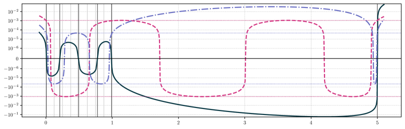
Figure 1: Comparison of errors of degree 5 polynomial approximations to $f(x)=\exp(-x)$. Legend: Lanczos-FA approximation for $\mathbf{b}$ with equal projection onto all eigenvectors of $\mathbf{A}$ (), optimal uniform approximation on $[0,5]$ (), optimal uniform approximation on $[0,1]\cup\{\mu^{*},5\}$ (). The light vertical lines are the eigenvalues of $\mathbf{A}$, while the darker vertical lines are the eigenvalues of $\mathbf{T}_{6}$ (the Ritz values). Remarks: Note that the Lanczos-FA approximation becomes very inaccurate on $(1,5)$ which allows a smaller error on the eigenvalues of $\mathbf{A}$, which is the only error that impacts our approximation to $f(\mathbf{A})\mathbf{b}$. As a result, the uniform approximation on $[0,1]\cup\{\mu^{*},5\}$ is a much better bound for the Lanczos-FA error than the uniform approximation on $[0,5]$, which remains equally accurate over the entire interval $[0,5]$.

1.2 Our Approach and Roadmap

Given the potential looseness of the classic uniform error bound on Lanczos-FA Eq. 3, our goal is to derive tighter, but still practically computable error bounds. Ideally, we want bounds that are both generally applicable and easier to apply than e.g., the bound of Eq. 4 based on interlacing.

One important case where such bounds already exist is when $f(x)=1/x$ and $\mathbf{A}$ is positive definite. In this setting, tight a posteriori error bounds are easily obtained by computing the residual $\|\mathbf{A}\textup{{lan}}_{k}(f)-\mathbf{b}\|$, and moreover, much stronger a priori error bounds are known than Eq. 3. In particular, $\|f(\mathbf{A})\mathbf{b}-\textup{{lan}}_{k}(f)\|$ is equal to the error of the conjugate gradient algorithm (CG) used to solve $\mathbf{A}\mathbf{x}=\mathbf{b}$ and therefore optimal over the Krylov subspace in the $\mathbf{A}$-norm. This immediately implies a priori bounds depending only on $\min_{\deg p<k}\|f-p\|_{\Lambda(\mathbf{A})}$, and so can be much tighter than Eq. 3 for matrices with clustered or isolated eigenvalues (see Appendix A for details).

Our approach is inspired by these sharper a posteriori and a priori error bounds for Lanczos-FA in the case of linear systems – i.e., for $f(x)=1/x$. We exploit the existence of these bounds to address a more general class of functions by using the Cauchy integral formula to write the Lanczos-FA error $f(\mathbf{A})\mathbf{b}-\textup{{lan}}_{k}(f)$ for any analytic $f$ in terms of the Lanczos error for solving a continuum of shifted linear systems in $\mathbf{A}$. We then bound this error in terms of the error in computing the solution to a single shifted system, $(\mathbf{A}-w\mathbf{I})^{-1}\mathbf{b}$. This reduction is presented in Section 2, along with a discussion of related work. We proceed, in Section 3, to show how this reduction can be used to obtain useful a priori and a posteriori error bounds. One highlight result is a proof that, for any analytic function $f$, the relative error of Lanczos-FA in approximating $f(\mathbf{A})\mathbf{b}$ can be bounded by a fixed constant times the relative error in solving a slightly shifted linear system in $\mathbf{A}$. We provide examples and numerical experiments that illustrate the quality of our bounds in Section 4. In Section 5 we give an analysis of our bounds in finite precision. Finally, in Section 6, we discuss generalizations to quadratic forms $\mathbf{b}^{\textup{{H}}}f(\mathbf{A})\mathbf{b}$.

2 Lanczos-FA error and the Cauchy integral formula

Assuming $f:\mathbb{C}\rightarrow\mathbb{C}$ is analytic in a neighborhood of the eigenvalues of $\mathbf{A}$ and $\Gamma$ is a simple closed curve or union of simple closed curves inside that neighborhood and enclosing the eigenvalues of $\mathbf{A}$, the Cauchy integral formula states that

(6) $$f(\mathbf{A})\mathbf{b}=-\frac{1}{2\pi i}\oint_{\Gamma}f(z)(\mathbf{A}-z\mathbf{I})^{-1}\mathbf{b}\,\mathrm{d}z.$$

If $\Gamma$ also encloses the eigenvalues of $\mathbf{T}_{k}$ we can similarly write the Lanczos-FA approximation as

(7) $$\mathbf{Q}_{k}f(\mathbf{T}_{k})\mathbf{Q}_{k}^{\textup{{H}}}\mathbf{b}=-\frac{1}{2\pi i}\oint_{\Gamma}f(z)\mathbf{Q}_{k}(\mathbf{T}_{k}-z\mathbf{I})^{-1}\mathbf{Q}_{k}^{\textup{{H}}}\mathbf{b}\,\mathrm{d}z.$$

Observing that the integrand of Eq. 6 contains the solution to the shifted linear system $(\mathbf{A}-z\mathbf{I})\mathbf{x}=\mathbf{b}$ while Eq. 7 contains the Lanczos-FA approximation to the solution, we make the following definition.

Definition 2.1.

For $z\in\mathbb{C}$, define the $k$-th Lanczos-FA error and residual for the linear system $(\mathbf{A}-z\mathbf{I})\mathbf{x}=\mathbf{b}$ as,

$$\textup{{err}}_{k}(z,\mathbf{A},\mathbf{b}) :=(\mathbf{A}-z\mathbf{I})^{-1}\mathbf{b}-\mathbf{Q}_{k}(\mathbf{T}_{k}-z\mathbf{I})^{-1}\mathbf{Q}_{k}^{\textup{{H}}}\mathbf{b},$$

$$\textup{{res}}_{k}(z,\mathbf{A},\mathbf{b}) :=\mathbf{b}-(\mathbf{A}-z\mathbf{I})\mathbf{Q}_{k}(\mathbf{T}_{k}-z\mathbf{I})^{-1}\mathbf{Q}_{k}^{\textup{{H}}}\mathbf{b}.$$

As with the Lanczos-FA approximation, we will typically omit the arguments $\mathbf{A}$ and $\mathbf{b}$, and in the case $z=0$, we will often write $\textup{{err}}_{k}$ and $\textup{{res}}_{k}$.

With Definition 2.1 in place, the error of the Lanczos-FA approximation to $f(\mathbf{A})\mathbf{b}$ can be written as

(8) $$f(\mathbf{A})\mathbf{b}-\mathbf{Q}_{k}f(\mathbf{T}_{k})\mathbf{Q}_{k}^{\textup{{H}}}\mathbf{b} =-\frac{1}{2\pi i}\oint_{\Gamma}f(z)\,\textup{{err}}_{k}(z)\,\mathrm{d}z.$$

Therefore, if for every $z\in\Gamma$ we are able to understand the convergence of Lanczos-FA on the linear system $(\mathbf{A}-z\mathbf{I})\mathbf{x}=\mathbf{b}$, then this formula lets us understand the convergence of Lanczos-FA for $f(\mathbf{A})\mathbf{b}$. To simplify bounding Eq. 8, we will write $\textup{{err}}_{k}(z)$ for all $z\in\Gamma$ in terms of the error in solving a single shifted linear system.

To do this, we use the fact that the Lanczos factorization Eq. 1 can be shifted, even for complex $z$, to obtain

(9) $$(\mathbf{A}-z\mathbf{I})\mathbf{Q}_{k} =\mathbf{Q}_{k}(\mathbf{T}_{k}-z\mathbf{I})+\beta_{k}\mathbf{q}_{k+1}\mathbf{e}_{k}^{\textup{{T}}}.$$

That is, Lanczos applied to $(\mathbf{A},\mathbf{b})$ for $k$ steps produces output $\mathbf{Q}_{k}$ and $\mathbf{T}_{k}$ satisfying Eq. 1 while Lanczos applied to $(\mathbf{A}-z\mathbf{I},\mathbf{b})$ for $k$ steps produces output $\mathbf{Q}_{k}$ and $\mathbf{T}_{k}-z\mathbf{I}$ satisfying Eq. 9. Using this fact, we have the following well known lemma.

Lemma 2.2.

For all $z$ where $\mathbf{T}_{k}-z\mathbf{I}$ is invertible,

$$\textup{{res}}_{k}(z)=\left(\frac{(-1)^{k}}{\det(\mathbf{T}_{k}-z\mathbf{I})}\prod_{j=1}^{k}\beta_{j}\right)\|\mathbf{b}\|_{2}\>\mathbf{q}_{k+1}.$$

Proof 2.3.

From Eq. 9, and the fact that $\mathbf{Q}_{k}$’s first column is $\mathbf{b}/\|{\mathbf{b}}\|_{2}$, it is clear that,

$$(\mathbf{A}-z\mathbf{I})\mathbf{Q}_{k}(\mathbf{T}_{k}-z\mathbf{I})^{-1}\mathbf{Q}_{k}^{\textup{{H}}}\mathbf{b} =(\mathbf{A}-z\mathbf{I})\mathbf{Q}_{k}(\mathbf{T}_{k}-z\mathbf{I})^{-1}\|\mathbf{b}\|_{2}\mathbf{e}_{1}$$

$$=\mathbf{Q}_{k}\|\mathbf{b}\|_{2}\mathbf{e}_{1}+\beta_{k}\mathbf{q}_{k+1}\mathbf{e}_{k}^{\textup{{T}}}(\mathbf{T}_{k}-z\mathbf{I})^{-1}\|\mathbf{b}\|_{2}\mathbf{e}_{1}$$

$$=\mathbf{b}+\beta_{k}\mathbf{q}_{k+1}\mathbf{e}_{k}^{\textup{{T}}}(\mathbf{T}_{k}-z\mathbf{I})^{-1}\|\mathbf{b}\|_{2}\mathbf{e}_{1}.$$

Using the formula $(\mathbf{T}_{k}-z\mathbf{I})^{-1}=(1/\det(\mathbf{T}_{k}-z\mathbf{I}))\mbox{ adj}(\mathbf{T}_{k}-z\mathbf{I})$, we see that

$$\mathbf{e}_{k}^{\textup{{T}}}(\mathbf{T}_{k}-z\mathbf{I})^{-1}\mathbf{e}_{1}=\frac{(-1)^{k-1}}{\det(\mathbf{T}_{k}-z\mathbf{I})}\prod_{j=1}^{k-1}\beta_{j}.$$

We use Lemma 2.2 to relate $\textup{{err}}_{k}(z)$ to $\textup{{err}}_{k}(w)$ for any $z,w\in\mathbb{C}$.

Definition 2.4.

For $w,z\in\mathbb{C}$ define $h_{w,z}:\mathbb{R}\to\mathbb{C}$ and $h_{z}:\mathbb{R}\to\mathbb{C}$ by

$$h_{w,z}(x):=\frac{x-w}{x-z}, h_{z}(x):=\frac{1}{x-z}$$

Corollary 2.5.

For all $z,w\in\mathbb{C}$, where $\mathbf{A}-z\mathbf{I}$ and $\mathbf{A}-w\mathbf{I}$ are both invertible,

$$\textup{{err}}_{k}(z) =\det(h_{w,z}(\mathbf{T}_{k}))h_{w,z}(\mathbf{A})\,\textup{{err}}_{k}(w)$$

$$\textup{{res}}_{k}(z) =\det(h_{w,z}(\mathbf{T}_{k}))\,\textup{{res}}_{k}(w).$$

Proof 2.6.

By Lemma 2.2,

$$\det(\mathbf{T}_{k}-z\mathbf{I})\,\textup{{res}}_{k}(z)=\det(\mathbf{T}_{k}-w\mathbf{I})\,\textup{{res}}_{k}(w).$$

Thus,

$$\textup{{res}}_{k}(z)=\frac{\det(\mathbf{T}_{k}-w\mathbf{I})}{\det(\mathbf{T}_{k}-z\mathbf{I})}\,\textup{{res}}_{k}(w)=\det(h_{w,z}(\mathbf{T}_{k}))\,\textup{{res}}_{k}(w).$$

Noting that $\textup{{res}}_{k}(z)=(\mathbf{A}-z\mathbf{I})\,\textup{{err}}_{k}(z)$ and $\textup{{res}}_{k}(w)=(\mathbf{A}-w\mathbf{I})\textup{{err}}_{k}(w)$, we obtain the relation between the errors,

$$\textup{{err}}_{k}(z) =\det(h_{w,z}(\mathbf{T}_{k}))(\mathbf{A}-z\mathbf{I})^{-1}(\mathbf{A}-w\mathbf{I})\,\textup{{err}}_{k}(w)$$

$$=\det(h_{w,z}(\mathbf{T}_{k}))h_{w,z}(\mathbf{A})\,\textup{{err}}_{k}(w).$$

In summary, combining Eq. 8 and Corollary 2.5 we have the following corollary. This result is by no means new, and appears throughout the literature; see for instance [21] and [17, Theorem 3.4].

Corollary 2.7.

Suppose $\mathbf{A}$ is a Hermitian matrix and $f:\mathbb{C}\rightarrow\mathbb{C}$ is a function analytic in a neighborhood of the eigenvalues of $\mathbf{A}$ and $\mathbf{T}_{k}$, where $\mathbf{T}_{k}$ is the tridiagonal matrix output by Lanczos run on $\mathbf{A},\mathbf{b}$ for $k$ steps. Then, if $\Gamma$ is a simple closed curve or union of simple closed curves inside this neighborhood and enclosing the eigenvalues of $\mathbf{A}$ and $\mathbf{T}_{k}$ and $w\in\mathbb{C}$ is such that $w\not\in\Lambda(\mathbf{T}_{k})\cup\Lambda(\mathbf{A})$,

$$f(\mathbf{A})\mathbf{b}-\textup{{lan}}_{k}(f) =\left(-\frac{1}{2\pi i}\oint_{\Gamma}f(z)\det(h_{w,z}(\mathbf{T}_{k}))h_{w,z}(\mathbf{A})\mathrm{d}z\right)\,\textup{{err}}_{k}(w).$$

2.1 Bound on Lanczos-FA error in terms of linear system error

Our main result is a flexible bound for the Lanczos-FA error, obtained by bounding the integral in the right-hand side of Corollary 2.7. As we will see in Section 3, we can instantiate this theorem to obtain effective a priori and a posteriori error bounds in many settings.

Theorem 2.8.

Consider the setting of Corollary 2.7. If, additionally, for some $S_{0},S_{1},\ldots,S_{k}\subset\mathbb{R}$ we have $\Lambda(\mathbf{A})\subset S_{0}\$ and $\lambda_{i}(\mathbf{T}_{k})\in S_{i}$ for $i=1,\ldots,k$, then

$$\|f(\mathbf{A})\mathbf{b}-\textup{{lan}}_{k}(f)\|\leq\underbrace{\vphantom{\bigg{|}}\left(\frac{1}{2\pi}\oint_{\Gamma}|f(z)|\cdot\left(\prod_{i=1}^{k}\|h_{w,z}\|_{S_{i}}\right)\cdot\|h_{w,z}\|_{S_{0}}\!\cdot|\mathrm{d}z|\right)}_{\text{integral term}}\underbrace{\vphantom{\Bigg{|}}\|\textup{{err}}_{k}(w)\|.}_{\text{linear system error}}$$

The above bound depends on our choices of $\Gamma$, $w$, and the sets $S_{0},S_{1},\ldots,S_{k}$, which must contain the eigenvalues of $\mathbf{A}$ and $\mathbf{T}_{k}$. The sets $S_{0},S_{1},\ldots,S_{k}$ should be chosen based on the informatoin we have about $\mathbf{A}$ and $\mathbf{T}_{k}$. For example, we could take all these sets to be the eigenvalue range $\mathcal{I}(\mathbf{A})$. If we have more information a priori about the eigenvalues of $\mathbf{A}$, we can obtain a tighter bound by choosing smaller $S_{0}$, with correspondingly lower $\|h_{w,z}\|_{S_{0}}$. For an a posteriori bound, we can simply set $S_{i}=\{\lambda_{i}(\mathbf{T}_{k})\}$, for $i=1,\ldots,k$. This gives an optimal value for $\|h_{w,z}\|_{S_{i}}$. Both approaches are detailed in Section 3.

We emphasize that the integral term and linear system error term in the theorem are entirely decoupled. Thus, once the integral term is computed, bounding the error of Lanczos-FA for $f(\mathbf{A})\mathbf{b}$ is reduced to bounding $\|\textup{{err}}_{k}(w)\|$, and if the integral term can be bounded independently of $k$, Theorem 2.8 implies that, up to a constant factor, the Lanczos-FA approximation to $f(\mathbf{A})\mathbf{b}$ converges at least as fast as $\|\textup{{err}}_{k}(w)\|$.

Proof 2.9 (Proof of Theorem 2.8).

Applying the triangle inequality for integrals and the submultiplicativity of matrix norms to Corollary 2.7 we have

(10) $$\|f(\mathbf{A})\mathbf{b}-\textup{{lan}}_{k}(f)\|\leq\left(\frac{1}{2\pi}\oint_{\Gamma}|f(z)|\cdot|\det(h_{w,z}(\mathbf{T}_{k}))|\cdot\|h_{w,z}(\mathbf{A})\|_{2}\!\cdot|\mathrm{d}z|\right)\|\textup{{err}}_{k}(w)\|.$$

Next, since $\Lambda(\mathbf{A})\subseteq S_{0}$ then

$$\|h_{w,z}(\mathbf{A})\|_{2}=\max_{i=1,\ldots,n}|h_{w,z}(\lambda_{i}(\mathbf{A}))|\leq\|h_{w,z}\|_{S_{0}},$$

and similarly, if $\lambda_{i}(\mathbf{T}_{k})\in S_{i}$ for $i=1,\ldots,k,$ then

(11) $$|\!\det(h_{w,z}(\mathbf{T}_{k}))|=\left|\prod_{i=1}^{k}h_{w,z}(\lambda_{i}(\mathbf{T}_{k}))\right|\leq\prod_{i=1}^{k}\|h_{w,z}\|_{S_{i}}.$$

Combining these inequalities yields the result.

2.2 Comparison with previous work

Our framework for analyzing Lanczos-FA has four properties which differentiate it from past work: (i) it is applicable to a wide range of functions, (ii) it yields a priori bounds dependent on fine-grained properties of the spectrum of $\mathbf{A}$ such as clustered or isolated eigenvalues, (iii) it can be used a posteriori as a practical stopping criterion, and (iv) it is applicable when computations are carried out in finite precision arithmetic. To the best of our knowledge, no existing analysis satisfies more than two of these properties simultaneously. In this section, we provide a brief overview of the most relevant past work.

Most directly related to our framework is a series of works which also make use of the shift-invariance of Krylov subspaces when $f$ is a Stieltjes function [16, 19, 35] or a certain type of rational function [18, 20, 21]. These analyses are applicable a priori and a posteriori and in fact allow for corresponding error lower bounds as well. However, these bounds cannot be applied to more general functions, and the impact of a perturbed Lanczos recurrence in finite precision is not considered.

The most detailed generally applicable analysis is [45], which extends [13, 14] and studies Eq. 3 when Lanczos is run in finite precision. However, as discussed in Section 1.1, Eq. 3 is often too pessimistic in practice as it does not depend on the fine-grained properties about the distribution of eigenvalues. Another generally applicable analysis is [34], which suggests replacing $\textup{{err}}_{k}(z)$ with $\textup{{res}}_{k}(z)$ in Eq. 8. Since $\textup{{res}}_{k}(z)$ can be computed once the outputs of Lanczos have been obtained, the resulting integral can be computed (or at least approximated by a quadrature rule). However, this approach does not take into account the actual relationship between $\textup{{res}}_{k}(z)$ and $\textup{{err}}_{k}(z)$, and therefore gives only an estimate of the error, not a true bound. Another Cauchy integral formula based approach is [33] which shows that Lanczos-FA exhibits superlinear convergence for the matrix exponential and certain other specific analytic functions.

There are a variety of other bounds specialized to individual functions. For example, it is known that if $\mathbf{A}$ is nonnegative definite and $t>0$, then the error in the Lanczos-FA approximation for the matrix exponential $\exp(t\mathbf{A})\mathbf{b}$ can be related to the maximum over $s\in[0,t]$ of the error in the optimal approximation to $\exp(s\mathbf{A})\mathbf{b}$ over a Krylov space of slightly lower dimension [11]. More recent work involving the matrix exponential are [38, 37, 36]. There is also a range of work which analyzes the convergence of Lanczos-FA and related methods for computing the square root and sign functions [4, 5, 57].

3 Applying our framework

We proceed to show how to effectively bound the integral term of Theorem 2.8, to give a priori and a posteriori bounds on the Lanczos-FA error, assuming accurate bounds on $\|\textup{{err}}_{k}(w)\|$ are available. Throughout, we assume $w\in\mathbb{R}$ and we do not discuss in detail how to bound this linear system error – there are many known approaches, both a priori and a posteriori, and the best bounds to use are often context dependent. For a more detailed discussion we refer readers to Appendix A.

To use Theorem 2.8, we must evaluate or bound $\|h_{w,z}\|_{S_{i}}$. Towards this end, we introduce the following lemmas, which apply when $S_{i}$ is an interval. These lemmas are also useful when $S_{i}$ is a union of intervals – in that case $\|h_{w,z}\|_{S_{i}}$ is bounded by the maximum bound on any of these intervals. i

Lemma 3.1.

For any interval $[a,b]\subset\mathbb{R}$, if $z\in\mathbb{C}\setminus[a,b]$ and $w\in\mathbb{R}$, we have

$$\|h_{w,z}\|_{[a,b]}=\max\left\{\left|\frac{a-w}{a-z}\right|,\left|\frac{b-w}{b-z}\right|,\left(\left|\frac{z-w}{\operatorname{Im}(z)}\right|~{}\text{ if }x^{*}\in[a,b]~{}\text{else}~{}0\right)\right\}$$

where

$$x^{*}:=\frac{\operatorname{Re}(z)^{2}+\operatorname{Im}(z)^{2}-\operatorname{Re}(z)w}{\operatorname{Re}(z)-w}.$$

Proof 3.2.

Note that for $x\in\mathbb{R}$,

$$|h_{w,z}(x)|^{2}=\left|\frac{x-w}{x-z}\right|^{2}=\frac{(x-w)^{2}}{(x-\operatorname{Re}(z))^{2}+\operatorname{Im}(z)^{2}},$$

and

$$\frac{\mathrm{d}missing}{\mathrm{d}x}\left(|h_{w,z}(x)|^{2}\right)=\frac{[(x-\operatorname{Re}(z))^{2}+\operatorname{Im}(z)^{2}]2(x-w)-(x-w)^{2}2(x-\operatorname{Re}(z))}{[(x-\operatorname{Re}(z))^{2}+\operatorname{Im}(z)^{2}]^{2}}.$$

Aside from $x=w$, where $h_{w,z}(x)=0$, the only value $x\in\mathbb{R}$ for which $\frac{\mathrm{d}missing}{\mathrm{d}x}\left(|h_{w,z}(x)|^{2}\right)=0$ is $x^{*}$. This implies that the only possible local extrema of $|h_{w,z}(x)|$ on $[a,b]$ are $a$, $b$, and $x^{*}$ if $x^{*}\in[a,b]$. Substituting the expression for $x^{*}$ into that for $|h_{w,z}(x^{*})|$, one finds, after some algebra, that $|h_{w,z}(x^{*})|=|z-w|/|\operatorname{Im}(z)|$.

Lemma 3.3.

Fix $r>0$, let $\mathcal{D}(c,t)$ be the disc in the complex plane centered at $c$ with radius $t\geq 0$, and define

$$X_{r}=\bigcup_{x\in[a,b]}\mathcal{D}\left(x,\frac{|x-w|}{r}\right).$$

Then for $z\in\mathbb{C}\setminus X_{r}$, we have

$$\|h_{w,z}\|_{[a,b]}\leq r.$$

In particular, if $z$ is on the boundary of $X_{r}$, then $\|h_{w,z}\|_{[a,b]}=r$.

Proof 3.4.

Let $z\in\mathbb{C}\setminus X_{r}$ and pick any $x\in[a,b]$. Since $z\not\in\mathcal{D}(x,|x-w|/r)$ it follows that $|z-x|>|x-w|/r$ and therefore $|h_{w,z}(x)|=|x-w|/|x-z|<r$. Maximizing over $x$ yields the result.

If $z$ is on the boundary of $X_{r}$, then for some $x\in[a,b]$, $|z-x|=|x-w|/r$, which means that for this $x$, $|h_{w,z}(x)|=r$.

Note that if $r\leq 1$ and $w\in\mathbb{R}\setminus[a,b]$, then the region described in Lemma 3.3 is simply a disc about $b$ if $w<a$ or a disc about $a$ if $w>b$. If $r>1$ and $w$ is real, then the region described is that in the discs about $a$ and $b$ and between the two external tangents to these two discs.

3.1 A priori bounds

We can use Theorem 2.8 to give a priori bounds, as long as we choose $S_{0}$ and $S_{i}$, $i=1,\ldots,k$ independently of $\mathbf{b}$ (and in turn $\mathbf{T}_{k}$).

The simplest possibility is to take $S_{0}=S_{i}=\mathcal{I}(\mathbf{A})$. In this case, as an immediate consequence of Theorems 2.8 and 3.3 we have the following a priori bound,

Corollary 3.5.

Suppose that for some $w<\lambda_{\textup{min}}(\mathbf{A})$, $f$ is analytic in a neighborhood of $\mathcal{D}(\lambda_{\textup{max}}(\mathbf{A}),\lambda_{\textup{max}}(\mathbf{A})-w)$. Then, taking $\Gamma$ to be the boundary of this disk,

$$\|f(\mathbf{A})\mathbf{b}-\textup{{lan}}_{k}(f)\| \leq\left(\frac{1}{2\pi}\oint_{\Gamma}|f(z)|\cdot|\mathrm{d}z|\right)\|\textup{{err}}_{k}(w)\|$$

$$\leq\left((\lambda_{\textup{max}}(\mathbf{A})-w)\>\max_{z\in\Gamma}|f(z)|\right)\|\textup{{err}}_{k}(w)\|.$$

Proof 3.6.

To obtain the first inequality observe that Lemma 3.3 with $[a,b]=\mathcal{I}(\mathbf{A})$ implies $\|h_{w,z}\|_{\mathcal{I}(\mathbf{A})}=1$ on this contour. The second inequality follows since the length of $\Gamma$ is $2\pi(\lambda_{\textup{max}}(\mathbf{A})-w)$.

This bound is closely related to [16, Theorem 6.6] which bounds the error in Lanczos-FA for Stieltjes functions in terms of the error in the Lanczos approximation for a certain linear system.

Using that $\textup{{err}}_{0}(w)=(\mathbf{A}-w\mathbf{I})^{-1}\mathbf{b}$, we can rewrite Corollary 3.5 as

$$\frac{\|f(\mathbf{A})\mathbf{b}-\textup{{lan}}_{k}(f)\|_{2}}{\|f(\mathbf{A})\mathbf{b}\|_{2}}\leq\max_{z\in\Gamma}|f(z)|\cdot\frac{(\lambda_{\textup{max}}(\mathbf{A})-w)\|(\mathbf{A}-w\mathbf{I})^{-1}\mathbf{b}\|_{2}}{\|f(\mathbf{A})\mathbf{b}\|_{2}}\cdot\frac{\|\textup{{err}}_{k}(w)\|_{2}}{\|\textup{{err}}_{0}(w)\|_{2}}.$$

This can be used to obtain simple relative error bounds for many functions. For instance, suppose $\mathbf{A}$ is positive definite, $f(x)=x^{-q}$ for $q>1$, and $w=c\lambda_{\text{min}}$ for $c\in(0,1)$. Then $\max_{z\in\Gamma}|z^{-q}|=w^{-q}=c^{-q}\lambda_{\textup{min}}(\mathbf{A})^{-q}$, $\|(\mathbf{A}-w\mathbf{I})^{-1}\mathbf{b}\|_{2}\leq(\lambda_{\textup{min}}(\mathbf{A})-w)^{-1}\|\mathbf{b}\|$ and $\|\mathbf{A}^{-q}\mathbf{b}\|_{2}\geq\lambda_{\textup{max}}(\mathbf{A})^{-q}\|\mathbf{b}\|$. We then have the bound

$$\frac{\|\mathbf{A}^{-q}\mathbf{b}-\textup{{lan}}_{k}(f)\|_{2}}{\|\mathbf{A}^{-q}\mathbf{b}\|_{2}} \leq c^{-q}\kappa(\mathbf{A})^{q}\kappa(\mathbf{A}-w\mathbf{I})\frac{\|\textup{{err}}_{k}(w)\|_{2}}{\|\textup{{err}}_{0}(w)\|_{2}}.$$

Corollary 3.5 and the above bound provide simple reductions to the error of solving a positive definite linear system involving $\mathbf{A}-w\mathbf{I}$ using Lanczos. However, these bounds may be a significant overestimate in practice. In particular, for any $k>1$, Eq. 11 cannot be sharp due to the fact that $\|h_{w,z}\|_{\mathcal{I}(\mathbf{A})}=\sup_{x\in\mathcal{I}(\mathbf{A})}|h_{w,z}(x)|$ cannot be attained at every eigenvalue of $\mathbf{T}_{k}$. In fact, for most values $\lambda_{i}(\mathbf{T}_{k})$ and most points $z\in\Gamma$, we expect $|h_{w,z}(\lambda_{i}(\mathbf{T}_{k}))|\ll\|h_{w,z}\|_{\mathcal{I}(\mathbf{A})}$. Figure 2 shows sample level curves for $\|h_{w,z}\|_{\mathcal{I}(\mathbf{A})}/|\det(h_{w,z}(\mathbf{T}_{k}))|^{1/k}$ which illustrate the slackness in the bound.

To derive sharper a priori bounds, there are several approaches. If more information is known about the eigenvalue distribution of $\mathbf{A}$, then the $S_{i}$ can be chosen based on this information. For example, similarly to Eq. 4, it is possible to exploit the interlacing property of the eigenvalues of $\mathbf{T}_{k}$.

Example 3.7.

Suppose $\mathbf{A}$ has eigenvalues in $[0,1]$ with a single eigenvalue at $\kappa>1$. Assume $w\leq 0$. Then there is at most one eigenvalue of $\mathbf{T}_{k}$ in $[1,\kappa]$ so in Theorem 2.8 we can pick $S_{i}=[0,1]$ for $i=1,\ldots,k-1$ and $S_{k}=[0,\kappa]$. We have

$$|\!\det(h_{w,z}(\mathbf{T}_{k}))|=\left|\prod_{i=1}^{k}h_{w,z}(\lambda_{i}(\mathbf{T}_{k}))\right|\leq\left(\|h_{w,z}\|_{[0,1]}\right)^{k-1}\|h_{w,z}\|_{[0,\kappa]}.$$

If $z$ is near to $\kappa$ then $\|h_{w,z}\|_{[0,1]}$ may be much smaller than $\|h_{w,z}\|_{[0,\kappa]}$.

Second, the contour $\Gamma$ can be chosen to try to reduce the slackness in Eq. 11. Intuitively, the slackness is exacerbated when $z\in\Gamma$ is close to $S_{i}$ but far from $\lambda_{i}(\mathbf{T}_{k})$. For instance, for any $k>1$,

$$\lim_{|z|\to\infty}\frac{\|h_{w,z}\|_{\mathcal{I}(\mathbf{A})}^{k}}{|\det(h_{w,z}(\mathbf{T}_{k}))|}\to 1, \forall\lambda\in\mathcal{I}(\mathbf{A}),~{}\lim_{z\to\lambda}\frac{\|h_{w,z}\|_{\mathcal{I}(\mathbf{A})}^{k}}{|\det(h_{w,z}(\mathbf{T}_{k}))|}\to\infty.$$ and

This behavior is also observed in Fig. 2.

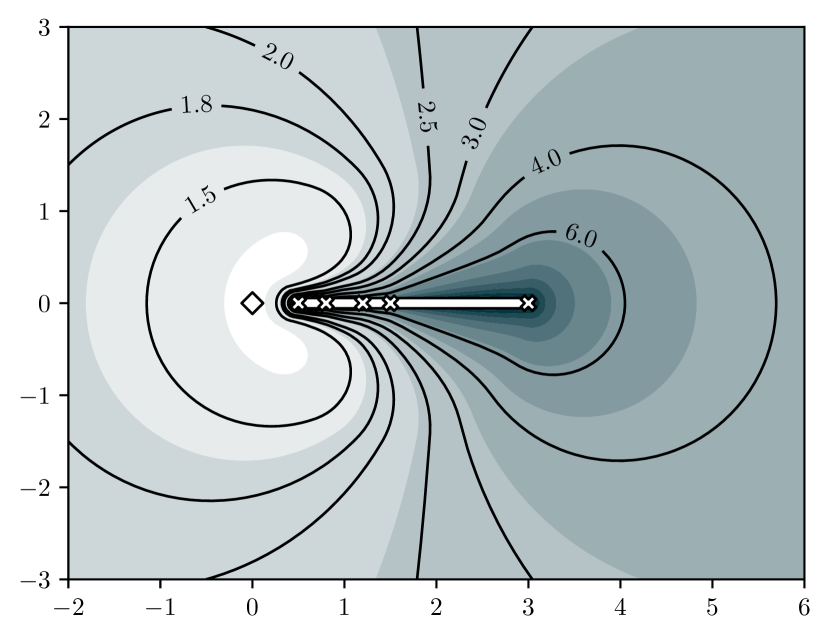
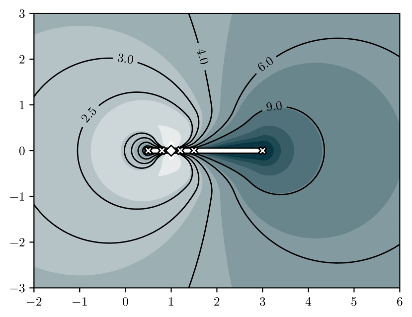
Figure 2: Contour plot of $\|h_{w,z}\|_{\mathcal{I}(\mathbf{A})}/|\!\det(h_{w,z}(\mathbf{T}_{k}))|^{1/k}$ as a function of $z\in\mathbb{C}$ for a synthetic example with $\mathcal{I}(\mathbf{A})=[0.5,3]$ and $\Lambda(\mathbf{T}_{k})=\{0.5,0.8,1.2,1.5,3\}$ ($k=5$). Here $w$ is indicated by the white diamond () and the eigenvalues of $\mathbf{T}_{k}$ are indicated by white x’s (). Larger slackness in Eq. 11 corresponds to darker regions.

These observations suggest that we should pick $\Gamma$ to be far from the spectrum of $\mathbf{A}$. Of course, we are constrained by properties of $f$ such as branch cuts and singularities. Moreover, certain contours may increase the slackness in Theorem 2.8 itself. These considerations are discussed further in Example 4.1.

3.2 A posteriori error bounds

After the Lanczos factorization Eq. 1 has been computed, $\mathbf{T}_{k}$ is known and $\Lambda(\mathbf{T}_{k})$ can be cheaply computed. Thus, in Theorem 2.8 we can take $S_{i}=\{\lambda_{i}(\mathbf{T}_{k})\}$ for $i=1,\ldots,k$, which is the best possible choice. In this case Eq. 11 is an equality and $\det(h_{w,z}(\mathbf{T}_{k}))=\det(\mathbf{T}_{k}-w)/\det(\mathbf{T}_{k}-z)$ can be computed via tridiagonal determinant formulas rather than using the eigenvalues of $\mathbf{T}_{k}$.

If $\mathcal{I}(\mathbf{A})$ is not known, the extreme Ritz values $\lambda_{\text{min}}(\mathbf{T}_{k})$ and $\lambda_{\text{max}}(\mathbf{T}_{k})$ can be used to estimate the extreme eigenvalues of $\mathbf{A}$ [40, 50]. All together, this means that it is not difficult to efficiently obtain accurate estimates of the bound from Theorem 2.8.

3.3 Numerical computation of integrals

Typically, to produce an a priori or a posteriori error bound, the integral term in Theorem 2.8 must be computed numerically. Consider a discretization of the integral

$$f(\mathbf{A})=-\frac{1}{2\pi i}\oint_{\Gamma}f(z)(\mathbf{A}-z\mathbf{I})^{-1}\mathrm{d}z$$

using nodes $z_{i}$ and weights $w_{i}$, $i=1,2,...,q$. This yields a rational matrix function

$$r_{q}(\mathbf{A}):=-\frac{1}{2\pi i}\sum_{i=1}^{q}w_{i}f(z_{i})(\mathbf{A}-z_{i}\mathbf{I})^{-1}.$$

Using the triangle inequality, we can write

$$\|f(\mathbf{A})\mathbf{b}-\textup{{lan}}_{k}(f)\|$$

$$\leq\|f(\mathbf{A})\mathbf{b}-r_{q}(\mathbf{A})\mathbf{b}\|+\|r_{q}(\mathbf{A})\mathbf{b}-\textup{{lan}}_{k}(r_{q}))\|+\|\textup{{lan}}_{k}(r_{q})-\textup{{lan}}_{k}(f)\|$$

(12) $$\leq 2\left(\max_{x\in\Lambda(\mathbf{A})\cup\Lambda(\mathbf{T}_{k})}|f(x)-r_{q}(x)|\right)\|\mathbf{b}\|+\|r_{q}(\mathbf{A})\mathbf{b}-\textup{{lan}}_{k}(r_{q})\|.$$

Now, observe that analogous to Theorem 2.8,

(13) $$\|r_{q}(\mathbf{A})\mathbf{b}-\textup{{lan}}_{k}(r_{q})\|\leq\left(\frac{1}{2\pi}\sum_{i=1}^{q}w_{i}\cdot|f(z_{i})|\cdot\left(\prod_{i=1}^{k}\|h_{w,z}\|_{S_{i}}\right)\cdot\|h_{w,z}\|_{S_{0}}\right)\|\textup{{err}}_{k}(w)\|.$$

If we use the same nodes and weights to evaluate the integral term in Theorem 2.8, we obtain exactly the expression on the right hand side of Eq. 13. Thus, this discretization of Theorem 2.8 is a true upper bound for the Lanczos-FA error to within an additive error of size equal to twice the approximation error of $r(x)$ to $f(x)$ on $\Lambda(\mathbf{A})\cup\Lambda(\mathbf{T}_{k})$ times $\|\mathbf{b}\|$. In many cases, we expect exponential convergence of $r_{q}$ to $f$, which implies that this term can be made less than any desired value $\epsilon>0$ using a number of quadrature nodes that grows only as the logarithm of $\epsilon^{-1}$ [30, 55].

We note that fast convergence of $r_{q}$ to $f$ suggests that, instead of applying Lanczos-FA, we can approximate $f(\mathbf{A})\mathbf{b}$ by first finding $r_{q}$ and then solving a small number of linear systems $(\mathbf{A}-z_{i}\mathbf{I})\mathbf{x}_{i}=\mathbf{b}$ to compute $r_{q}(\mathbf{A})\mathbf{b}$. Solving these systems with any fast linear system solver yields an algorithm for approximating $f(\mathbf{A})\mathbf{b}$ inheriting, up to logarithmic factors in the error tolerance, the same convergence guarantees as the linear system solvers used. A recent example of this approach is found in [39] which uses a modified version of stochastic variance reduced gradient (SVRG) to obtain a nearly input sparsity time algorithm for $f(\mathbf{A})\mathbf{b}$ when $f$ corresponds to principal component projection or regression.

A range of work suggests using a Krylov subspace method and the shift invariance of the Krylov subspace to solve these systems and compute $r_{q}(\mathbf{A})\mathbf{b}$ explicitly. This was studied in [18, 21] for the Lanczos method, and in [51] for MINRES, the latter of which uses the results of [30] to determine the quadrature nodes and weights. However, as the above argument demonstrates, the limit of the Lanczos-based approximation as the discretization becomes finer is simply the Lanczos-FA approximation to $f(\mathbf{A})\mathbf{b}$. Therefore, there is no clear advantage to such an approach over Lanczos-FA in terms of the convergence properties, unless preconditioning is used. .

On the other hand, there are some advantages to these approaches in terms of computation. Indeed, Krylov solvers for symmetric/Hermitian linear systems require just $O(n)$ storage; i.e. they do not require more storage as more iterations are taken. A naive implementation of Lanczos-FA requires $O(kn)$ storage, and while Lanczos-FA can be implemented to use $O(n)$ storage by taking two passes, this has the effect of doubling the number of matrix-vector products required. See [29] for a recent overview of limited-memory Krylov subspace methods.

4 Examples and numerical verification

We next present examples in which we apply Theorem 2.8 to give a posteriori and a priori error bounds for approximating common matrix functions with Lanczos-FA. These examples illustrate the general approaches to applying Theorem 2.8 described in Section 3. All integrals are computed either analytically or using SciPy’s integrate.quad which is a wrapper for QUADPACK routines.

In all cases, we exactly compute the $\|\textup{{err}}_{k}(w)\|$ term in the bounds. In practice, one would bound this quantity a priori or a posteriori using existing results on bounding the Lanczos error for linear system solves. By computing the error exactly, we separate any looseness due to our bounds from any looseness due to an applied bound on $\|\textup{{err}}_{k}(w)\|$.

Example 4.1 (Matrix square root).

Let $\mathbf{A}$ be positive definite and $f(x)=\sqrt{x}$. Perhaps the simplest bound is obtained by using Theorem 2.8 with $w=0$, $S_{i}=\mathcal{I}(\mathbf{A})$ and $\Gamma$ chosen as the boundary of the disk $\mathcal{D}(\lambda_{\text{max}}(\mathbf{A}),\lambda_{\text{max}}(\mathbf{A}))$.We then obtain a bound via Corollary 3.5. However, this bound may be loose – note that except through $\|\textup{{err}}_{k}(w)\|$, it does not depend on the number of iterations $k$. Thus it cannot establish convergence at a rate faster than that of solving a linear system with coefficient matrix $\mathbf{A}$.

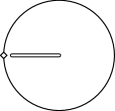
(a) circle contour

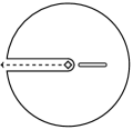
(b) Pac-Man contour

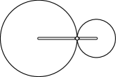
(c) double circle contour

Figure 3: Circle, Pac-Man and double circle contours described in Examples 4.1 and 4.2 respectively. All three figures show $\mathcal{I}(\mathbf{A})$ () and $w$ ().

Keeping $w=0$, we can obtain tighter bounds by letting $\Gamma$ be a “Pac-Man” like contour that consists of a large circle about the origin of radius $R$ with a small circular cutout of radius $r$ that excludes the origin and a small strip cutout to exclude the negative real axis. That is, as shown in Fig. 3(b), the boundary of the set,

$$\mathcal{D}(0,R)\setminus(\{z:\operatorname{Re}(z)\leq 0,|\operatorname{Im}(z)|<r\}\cup\mathcal{D}(0,r)).$$

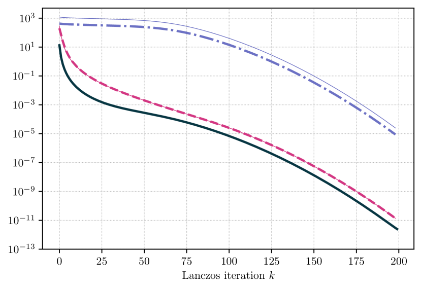
(a) circular contour ($c=r=\lambda_{\text{max}}(\mathbf{A})$)

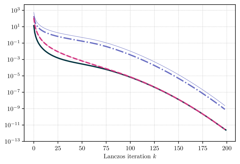
(b) Pac-Man contour ($r\rightarrow 0$, $R\rightarrow\infty$)

Figure 4: $\mathbf{A}$-norm error bounds for $f(x)=\sqrt{x}$ where $\mathbf{A}$ has $n=1000$ eigenvalues spaced uniformly in $[10^{-2},10^{2}]$. Legend: True Lanczos-FA error $\|f(\mathbf{A})\mathbf{b}-\textup{{lan}}_{k}(f)\|$ (). A priori bounds obtained by using Theorem 2.8 with $S_{0}=S_{i}=\mathcal{I}(\mathbf{A})$ () and $S_{0}=S_{i}=\tilde{\mathcal{I}}(\mathbf{A})=[\lambda_{\text{min}}(\mathbf{A})/2,2\lambda_{\text{max}}(\mathbf{A})]$ (). A posteriori bounds obtained by using Theorem 2.8 with $S_{0}=\mathcal{I}(\mathbf{A})$, $S_{i}=\{\lambda_{i}(\mathbf{T}_{k})\}$ (), and $S_{0}=\tilde{\mathcal{I}}(\mathbf{A})$, $S_{i}=\{\lambda_{i}(\mathbf{T}_{k})\}$ (). Observe that using the wider interval $\tilde{\mathcal{I}}(\mathbf{A})$ has very little effect on both the a priori and a posteriori bounds. Also observe that the a posteriori bounds closely match the actual convergence of Lanczos-FA.

As the outer radius $R\rightarrow\infty$, the integral over the large circular arc goes to $0$ since $\|h_{w,z}\|_{\mathcal{I}(\mathbf{A})}=O(R^{-1})$, $|f(z)|=O(R^{1/2})$, and the length of the circular arc is on the order of $R$. Thus, the product $f(z)(\|h_{w,z}\|_{\mathcal{I}(\mathbf{A})})^{k+1}$ goes to $0$ as $R\rightarrow\infty$, for all $k\geq 1$. Similarly, as $r\to 0$, the length of the small arc goes to zero. Therefore, we need only consider the contributions to the integral on $[-R\pm ir,\pm ir]$ in the limit $R\to\infty,r\to 0$.

In this case, when $S_{i}=\mathcal{I}(\mathbf{A})$ for all $i$, we can compute the value of the integral term in Theorem 2.8 analytically. We have

$$\|f(\mathbf{A})\mathbf{b}-\textup{{lan}}_{k}(f)\| \leq\left(\frac{1}{2\pi}\int_{-\infty}^{0}|(x\pm 0i)^{1/2}|\cdot\|h_{w,x\pm 0i}\|_{\mathcal{I}(\mathbf{A})}^{k+1}\,\mathrm{d}x\right)\|\textup{{err}}_{k}\|$$

$$=\left(\frac{1}{2\pi}\int_{-\infty}^{0}|x\pm 0i|^{1/2}\frac{\lambda_{\text{max}}(\mathbf{A})^{k+1}}{(\lambda_{\text{max}}(\mathbf{A})-x)^{k+1}}\,\mathrm{d}x\right)\|\textup{{err}}_{k}\|$$

$$=\left(\frac{1}{\pi}\lambda_{\text{max}}(\mathbf{A})^{k+1}\int_{0}^{\infty}\frac{y^{1/2}}{(\lambda_{\text{max}}(\mathbf{A})+y)^{k+1}}\mathrm{d}y\right)\|\textup{{err}}_{k}\|$$

$$=\left(\frac{\lambda_{\text{max}}(\mathbf{A})^{3/2}}{2\sqrt{\pi}}\frac{\Gamma(k-1/2)}{\Gamma(k+1)}\right)\|\textup{{err}}_{k}\|,$$

where we have made the change of variable $y=-x$. Note that

$$\lim_{k\to\infty}k^{3/2}\frac{\Gamma(k-1/2)}{\Gamma(k+1)}=1.$$

This proves that $\textup{{lan}}_{k}(\sqrt{\cdot})$ converges somewhat faster than the Lanczos algorithm applied to the corresponding linear system $\mathbf{A}\mathbf{x}=\mathbf{b}$.

In Fig. 4, we plot the bounds from Theorem 2.8 for the circular and Pac-Man contours described above. For both contours we consider $S_{i}=\mathcal{I}(\mathbf{A})$ for all $i$, as well as bounds based on an overestimate of this interval, $S_{i}=\tilde{\mathcal{I}}(\mathbf{A})$ where $\tilde{\mathcal{I}}(\mathbf{A})=[\lambda_{\text{min}}(\mathbf{A})/2,2\lambda_{\text{max}}(\mathbf{A})].$ This provides some sense of how sensitive the bounds are to the choice of $S_{i}$ when $S_{i}$ is a single interval. For a posteriori bounds, we set $S_{i}$ to $\{\lambda_{i}(\mathbf{T}_{k})\}$ for $i>0$.

We remark that the bounds from Theorem 2.8 are upper bounds for Eq. 10 which implies that the slackness of Eq. 10 is relatively small. This suggests that the roughly 6 orders of magnitude improvement in Theorem 2.8 when moving from the circular contour to the Pac-Man contour is primarily due to reducing the slackness in Eq. 11, aligning with our intuition.

(a) $(\mathbf{A}-w\mathbf{I})^{2}$-norm for $f(x)=\operatorname{step}(x-a)/x$ where $\mathbf{A}=\mathbf{X}\mathbf{X}^{\textup{{H}}}$ and the entries of $\mathbf{X}\in\mathbb{R}^{n,2n}$ are independent Gaussians with mean zero and variance $1/2n$ with $n=3000$. We set $a=0.99\lambda_{\text{max}}(\mathbf{A})$ so that there are roughly $5$ eigenvalues above $a$.

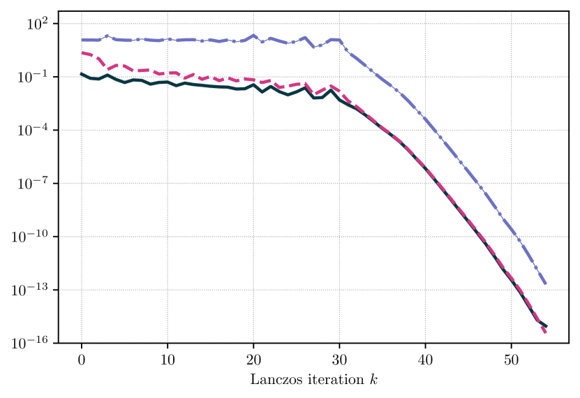
(b) $2$-norm for $f(x)=\operatorname{step}(x-a)$ where $\mathbf{A}$ is the MNIST training data [41] covariance matrix and $a=0.15\lambda_{\text{max}}(\mathbf{A})$ so that there are 16 eigenvalues above $a$.

Figure 5: Bounds for piece-wise analytic functions using the double-circle contour described in Example 4.2. Legend: True Lanczos-FA error (). A priori bounds obtained by using Theorem 2.8 with $S_{0}=S_{i}=\mathcal{I}(\mathbf{A})$ () or Eq. 14 () with $S_{0}=S_{i}=\mathcal{I}(\mathbf{A})$. Note that these curves are on top of one another suggesting there is very little loss going from Theorem 2.8 to the much easier to evaluate Eq. 14. An a posteriori bound obtained by using Theorem 2.8 with $S_{0}=\mathcal{I}(\mathbf{A})$ and $S_{i}=\{\lambda_{i}(\mathbf{T}_{k})\}$ (). Observe that all bounds, especially the a posteriori ones closely match the true convergence of Lanczos-FA.

Our next example illustrates the application of Theorem 2.8 to several common piecewise analytic functions. Functions of this class have found widespread use throughout scientific computing and data science but have proven particularly difficult to analyze using existing approaches [10, 22, 39, 57].

Example 4.2 (Step and Absolute Value Functions).

Let $f(x)$ be one of $|x-a|$, $\operatorname{step}(x-a)$, or $\operatorname{step}(x-a)/x$ for $a\in\mathcal{I}(\mathbf{A})$, where, for $z\in\mathbb{C}$ we define $\operatorname{step}(z):=0$ for $\text{Re}(z)<0$ and $\operatorname{step}(z):=1$ for $\text{Re}(z)\geq 0$. Also, for $z\in\mathbb{C}$, we replace $|x-a|$ by $z-a$ if $\text{Re}(z)>a$ and by $a-z$ if $\text{Re}(z)\leq a$. Note that the latter two functions correspond to principle component projection and principle component regression respectively. In the case of principle component regression, we $\mathbf{A}$ is positive semi-definite. The step function is also closely related to the sign function, which is widely used in quantum chromodynamics to compute the overlap operator [57].

Next, take $w=a$ and define $\Gamma_{1}$ and $\Gamma_{2}$ as the boundaries of the disks $\mathcal{D}_{1}:=\mathcal{D}(\lambda_{\text{min}}(\mathbf{A}),w-\lambda_{\text{min}}(\mathbf{A})-\varepsilon)$ and $\mathcal{D}_{2}:=\mathcal{D}(\lambda_{\text{max}}(\mathbf{A}),\lambda_{\text{max}}(\mathbf{A})-w-\varepsilon)$, for some sufficiently small $\varepsilon>0$. Then $f$ is analytic in a neighborhood of the union of these two disks, so assuming none of the eigenvalues of $\mathbf{A}$ or $\mathbf{T}_{k}$ are equal to $a$, we can apply Lemma 3.3.

Note that $\|h_{w,z}\|_{\mathcal{I}(\mathbf{A})}\to 1$ as $z\to w$ from outside $[a,b]$, avoiding a potential singularity which would occur if the contour $\Gamma$ passed through $\mathcal{I}(\mathbf{A})$ at any other points. In fact, ignoring the contribution of $\epsilon$, $\|h_{w,z}\|_{\mathcal{I}(\mathbf{A})}=1$ for all $z\in\Gamma_{1}$ and for all $z\in\Gamma_{2}$. Thus, Corollary 3.5 can be written as

(14) $$\|f(\mathbf{A})\mathbf{b}-\textup{{lan}}_{k}(f)\| \leq\left(\frac{1}{2\pi}\sum_{j=1}^{2}|\Gamma_{j}|\max_{z\in\Gamma_{j}}|f(z)|\right)\|\textup{{err}}_{k}(w)\|.$$

The values of this bound for all three functions are summarized in Table 1.

In Fig. 5, we plot the bounds from Theorem 2.8 for the contour described above with $S_{i}=\mathcal{I}(\mathbf{A})$.

$$\begin{array}[]{rlll}\hline\cr\hline\cr f(x)&f(z),z\in\Omega_{1}&f(z),z\in\Omega_{2}&\frac{1}{2\pi}\sum_{j=1}^{2}|\Gamma_{j}|\max_{z\in\Gamma_{j}}|f(z)|\\ \hline\cr|x-a|&a-z&z-a&2(a-\lambda_{\text{min}})^{2}+2(\lambda_{\text{max}}-a)^{2}\\ \operatorname{step}(x-a)&0&1&(\lambda_{\text{max}}-a)\\ \operatorname{step}(x-a)/x&0&1/z&(\lambda_{\text{max}}-a)/a\\ \hline\cr\hline\cr\end{array}$$

Table 1: Values of the factor in parentheses on the right-hand side of Eq. 14 (ignoring $\varepsilon$) for several common piecewise analytic functions.

If $w\in\mathcal{I}(\mathbf{A})$ we note that $\|\textup{{err}}_{k}(w)\|$ corresponds to the indefinite linear system $(\mathbf{A}-w\mathbf{I})\mathbf{x}=\mathbf{b}$, so standard results for the Conjugate Gradient algorithm are not applicable. However, the residual of this system can still be computed exactly once the Lanczos factorization Eq. 1 has been obtained, and as we prove in Appendix A, a priori bounds for the convergence of MINRES [8] can be extended to the Lanczos algorithm for indefinite systems. It is also clear that, at the cost of having to compare against the error of multiple different linear systems, functions which are piecewise analytic on more than two regions can be handled.

5 Finite precision

While reorthogonalization in the Lanczos method (Algorithm 1) is unnecessary in exact arithmetic, omitting it may result in drastically different behavior when using finite precision arithmetic; see for instance [43]. In the context of Lanczos-FA, the two primary effects are (i) a delay of convergence (increase in the number of iterations to reach a given level of accuracy) and (ii) a reduction in the maximal attainable accuracy. These effects are reasonably well understood in the context of linear systems [25, 26], i.e., $f(x)=1/x$, and for some other functions such as the matrix exponential [11]. However, general theory is limited. A notable exception is [45], which argues that the uniform error bound for Lanczos-FA Eq. 3 holds to a close degree in finite precision arithmetic.

When run without reorthogonlization, Algorithm 1 will produce $\mathbf{Q}_{k}$ and $\mathbf{T}_{k}$ satisfying a perturbed three term recurrence

(15) $$\mathbf{A}\mathbf{Q}_{k}=\mathbf{Q}_{k}\mathbf{T}_{k}+\beta_{k}\mathbf{q}_{k+1}\mathbf{e}_{k}^{\textup{{T}}}+\mathbf{F}_{k},$$

where $\mathbf{F}_{k}$ is a perturbation term. Moreover, the columns of $\mathbf{Q}_{k}$ may no longer be orthogonal. A priori bounds on the size of $\mathbf{F}_{k}$ and the loss of orthogonality between successive Lanczos vectors have been established in a series of works by Paige [46, 47, 48, 49]. These quantities can also be computed easily once $\mathbf{Q}_{k}$ and $\mathbf{T}_{k}$ have been obtained, allowing for easy use with our bounds.

5.1 Effects of finite precision on our error bounds for Lanczos-FA

Note that using the divide and conquer algorithm from [28] to compute the eigendecomposition of the tridiagonal matrix $\mathbf{T}_{k}$, we can quickly and stably compute $\mathbf{Q}_{k}f(\mathbf{T}_{k})\mathbf{e}_{1}$. A detailed analysis of this is given in [45, Appendix A].

While the tridiagonal matrix $\mathbf{T}_{k}$ and the matrix $\mathbf{Q}_{k}$ of Lanczos vectors produced in finite precision arithmetic may be very different from those produced in exact arithmetic, we now show that our error bounds, based on the $\mathbf{T}_{k}$ and $\mathbf{Q}_{k}$ actually produced, still hold to a close approximation. First, we argue that Lemma 2.2 holds to a close degree provided $\mathbf{F}_{k}$ is not too large. Towards this end, note that we have the shifted perturbed recurrence,

(16) $$(\mathbf{A}-z\mathbf{I})\mathbf{Q}_{k} =\mathbf{Q}_{k}(\mathbf{T}_{k}-z\mathbf{I})+\beta_{k}\mathbf{q}_{k+1}\mathbf{e}_{k}^{\textup{{T}}}+\mathbf{F}_{k}.$$

From Eq. 16, it is then clear that,

$$(\mathbf{A}-z\mathbf{I})\mathbf{Q}_{k}(\mathbf{T}_{k}-z\mathbf{I})^{-1}\mathbf{e}_{1} =\mathbf{Q}_{k}\mathbf{e}_{1}+\beta_{k}\mathbf{q}_{k+1}\mathbf{e}_{k}^{\textup{{T}}}(\mathbf{T}_{k}-z\mathbf{I})^{-1}\mathbf{e}_{1}+\mathbf{F}_{k}(\mathbf{T}_{k}-z\mathbf{I})^{-1}\mathbf{e}_{1}.$$

This implies that Corollary 2.5 also holds closely. More specifically,

$$\textup{{res}}_{k}(z) =\det(h_{w,z}(\mathbf{T}_{k}))\textup{{res}}_{k}(w)+\mathbf{f}_{k}(w,z)$$

$$\textup{{err}}_{k}(z) =\det(h_{w,z}(\mathbf{T}_{k}))h_{w,z}(\mathbf{A})\textup{{err}}_{k}(w)+(\mathbf{A}-z\mathbf{I})^{-1}\mathbf{f}_{k}(w,z)$$

where

$$\mathbf{f}_{k}(w,z):=\mathbf{F}_{k}\left((\mathbf{T}_{k}-z\mathbf{I})^{-1}-\det(h_{w,z}(\mathbf{T}_{k}))(\mathbf{T}_{k}-w\mathbf{I)}^{-1}\right)\mathbf{e}_{1}.$$

Using this we have,

$$f(\mathbf{A})\mathbf{b}-\textup{{lan}}_{k}(f) =-\frac{1}{2\pi i}\oint_{\Gamma}f(z)\textup{{err}}_{k}(z)\mathrm{d}z-\frac{1}{2\pi i}\oint_{\Gamma}f(z)(\mathbf{A}-z\mathbf{I})^{-1}\mathbf{f}_{k}(w,z)\mathrm{d}z$$

which we may bound using the triangle inequality as

$$\|f(\mathbf{A})\mathbf{b}-\textup{{lan}}_{k}(f)\| \leq\frac{1}{2\pi}\left\|\oint_{\Gamma}f(z)\textup{{err}}_{k}(z)\mathrm{d}z\right\|+\frac{1}{2\pi}\left\|\oint_{\Gamma}f(z)(\mathbf{A}-z\mathbf{I})^{-1}\mathbf{f}_{k}(w,z)\mathrm{d}z\right\|.$$

This expression differs from Theorem 2.8 only by the presence of the term involving $\mathbf{f}_{k}(w,z)$ (and, of course, by the fact that $\textup{{err}}_{k}(z)$ now denotes the error in the finite precision computation). If we take $\|\cdot\|$ as the $(\mathbf{A}-w\mathbf{I})^{2}$-norm, then this additional term can be bounded by,

$$\frac{1}{2\pi}\left\|\oint_{\Gamma}f(z)(\mathbf{A}-z\mathbf{I})^{-1}\mathbf{f}_{k}(w,z)\mathrm{d}z\right\|$$

$$\leq\frac{1}{2\pi}\oint_{\Gamma}|f(z)|\cdot\|(\mathbf{A}-w\mathbf{I})(\mathbf{A}-z\mathbf{I})^{-1}\|_{2}\cdot\|\mathbf{f}_{k}(w,z)\|_{2}\cdot|\mathrm{d}z|$$

(17) $$\leq\frac{1}{2\pi}\oint_{\Gamma}|f(z)|\cdot\|h_{w,z}\|_{S_{0}}\cdot\|\mathbf{f}_{k}(w,z)\|_{2}\cdot|\mathrm{d}z|.$$

Note that Eq. 17 can be viewed as an upper bound of the ultimate obtainable accuracy of Lanczos-FA in finite precision after convergence. If the inequalities do not introduce too much slack, this upper bound will also produce a reasonable estimate. If $\|\mathbf{F}_{k}\|$ is small, the size of this addition is also hopefully small, in which case one may simply ignore the contribution of Eq. 17, provided the Lanczos-FA error is not near the final accuracy. We have worked in the $(\mathbf{A}-w\mathbf{I})^{2}$ norm as it simplifies some of the analysis, but in principle, a similar approach could be used with other norms. This is straightforward, but would involve bounding something other than $\|h_{w,z}\|_{S_{0}}$.

Example 5.1.

The left panel of Fig. 6 shows the convergence of Lanczos-FA when Algorithm 1, without reorthogonalization, is used to generate $\mathbf{Q}_{k}$ and $\mathbf{T}_{k}$. Compared with the error of the iterates generated using full orthogonalization, a delay of convergence and loss of accuracy are clear. This figure also shows the error bounds derived by bounding $\|\mathbf{F}_{k}\|$ as described above. We note that the contribution from the integral in Eq. 17 is almost negligible until the bound is near the final accuracy.

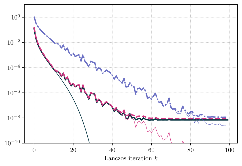
(a) $(\mathbf{A}-w\mathbf{I})^{2}$-norm error bounds for $f(x)=\sqrt{x}$ using a Pac-Man contour ($r\to 0$, $R\to\infty$). Legend: True Lanczos-FA error (). A priori bounds obtained by using Theorem 2.8 with $S_{0}=S_{i}=\mathcal{I}(\mathbf{A})$ with () and without () right hand side of Eq. 17. A posteriori bounds obtained by using Theorem 2.8 with $S_{0}=\mathcal{I}(\mathbf{A})$ and $S_{i}=\{\lambda_{i}(\mathbf{T}_{k})\}$ with () and without () right hand side of Eq. 17. For reference, the convergence of Lanczos-FA with reorthogonalization in double precision () is also shown.

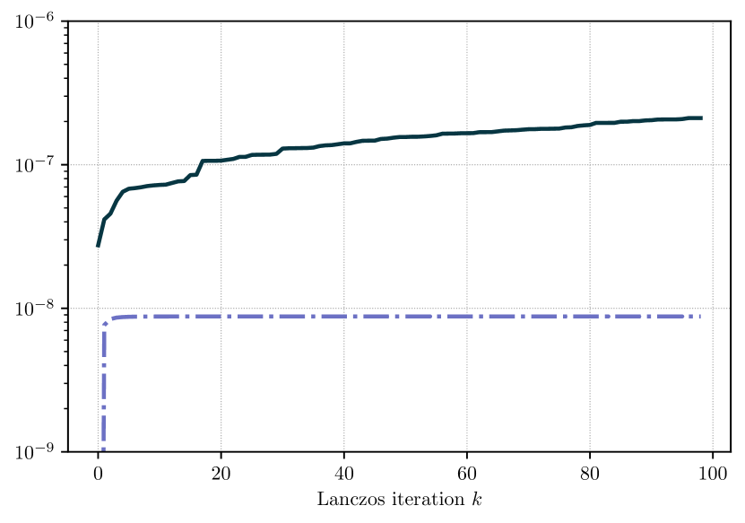
(b) Legend: $\|\mathbf{F}_{k}\|_{\mathsf{F}}$ (), right hand side of Eq. 17 (). Note that the size of $\mathbf{F}_{k}$ is small relative to the Lanczos-FA error, until the accuracy is near the final accuracy.

Figure 6: $\mathbf{A}$ has $n=50$ eigenvalues with $\lambda_{1}=1$, $\lambda_{n}=0.001$, and $\lambda_{i}=\lambda_{n}+\frac{n-i}{n-1}(\lambda_{1}-\lambda_{n})\rho^{i-1}$, $i=2,\ldots,n-1$, as described in [53] with parameter $\rho=0.8$. Here Lanczos is run without reorthogonalization in single precision arithmetic, but the integrals are evaluated using double precision arithmetic.

6 Quadratic forms

In many applications, one seeks to compute $\mathbf{b}^{\textup{{H}}}f(\mathbf{A})\mathbf{b}$ rather than $f(\mathbf{A})\mathbf{b}$. A common approach is Lanczos quadrature, which computes the approximation $\mathbf{b}^{\textup{{H}}}\textup{{lan}}_{k}(f)$ to $\mathbf{b}^{\textup{{H}}}f(\mathbf{A})\mathbf{b}$. This approximation is a degree $k$ Gaussian quadrature approximation to the integral of $f$ against the weighted spectral measure corresponding to $\mathbf{A},\mathbf{b}$; see for instance [7, 23, 56]. However, as with the case of Lanczos-FA, most existing error bounds for Lanczos quadrature are either pessimistic or limited to special classes of functions.

Note that the Lanczos-FA approximation satisfies,

$$\mathbf{b}^{\textup{{H}}}\textup{{lan}}_{k}(f)=\mathbf{b}^{\textup{{H}}}\mathbf{Q}_{k}f(\mathbf{T}_{k})\mathbf{Q}_{k}^{\textup{{H}}}\mathbf{b}=\|\mathbf{b}\|_{2}^{2}\>\mathbf{e}_{1}^{\textup{{H}}}f(\mathbf{T}_{k})\mathbf{e}_{1}.$$

Thus, we can compute $\mathbf{b}^{\textup{{H}}}\textup{{lan}}_{k}(f)$ without storing or recomputing $\mathbf{Q}_{k}$.

Since $\mathbf{A}$ is Hermitian, $(\mathbf{A}-z\mathbf{I})^{\textup{{H}}}=\mathbf{A}-\overline{z}\mathbf{I}$. Thus, since

$$\mathbf{b}^{\textup{{H}}}(\mathbf{A}-z\mathbf{I})^{-1}=((\mathbf{A}-\overline{z}\mathbf{I})^{-1}\mathbf{b})^{\textup{{H}}}=(\textup{{lan}}_{k}(h_{\overline{z}})+\textup{{err}}_{k}(\overline{z}))\mathbf{b})^{\textup{{H}}}$$

we can expand the quadratic form error as

$$\mathbf{b}^{\textup{{H}}}\textup{{err}}_{k}(z)=\mathbf{b}^{\textup{{H}}}(\mathbf{A}-z\mathbf{I})^{-1}\textup{{res}}_{k}(z)=\left(\textup{{lan}}_{k}(h_{\overline{z}}))+\textup{{err}}_{k}(\overline{z})\right)^{\textup{{H}}}\textup{{res}}_{k}(z).$$

Now, by definition, $\textup{{lan}}_{k}(h_{\overline{z}}(x))=\mathbf{Q}_{k}h_{\overline{z}}(\mathbf{T}_{k})\mathbf{Q}^{\textup{{H}}}\mathbf{b}$ and by Lemma 2.2 $\textup{{res}}_{k}(z)$ is proportional to $\mathbf{q}_{k+1}$. Thus, since, at least in exact arithmetic, $\mathbf{q}_{k+1}$ is orthogonal to $\mathbf{Q}_{k}$,

$$\mathbf{b}^{\textup{{H}}}\textup{{err}}_{k}(z) =\textup{{err}}_{k}(\overline{z})^{\textup{{H}}}\textup{{res}}_{k}(z)=((\mathbf{A}-\overline{z}\mathbf{I})^{-1}\textup{{res}}_{k}(\overline{z}))^{\textup{{H}}}\textup{{res}}_{k}(z).$$

Next, using Corollary 2.5 and the fact that $h_{w,z}(x)h_{w,\overline{z}}(x)=|h_{w,z}(x)|^{2}$ for $w,x\in\mathbb{R}$,

$$\mathbf{b}^{\textup{{H}}}\textup{{err}}_{k}(z) =|\det(h_{w,z}(\mathbf{T}_{k}))|^{2}\textup{{res}}_{k}(w)^{\textup{{H}}}(\mathbf{A}-z\mathbf{I})^{-1}\textup{{res}}_{k}(w).$$

We then have,

$$|\mathbf{b}^{\textup{{H}}}\textup{{err}}_{k}(z)|\leq|\!\det(h_{w,z}(\mathbf{T}_{k}))|^{2}\cdot\|(\mathbf{A}-z\mathbf{I})^{-1}\|_{2}\cdot\|\textup{{res}}_{k}(w)\|_{2}^{2}.$$

Applying the Cauchy integral formula we therefore obtain a bound for the quadratic form error analogous to Theorem 2.8,

(18) $$|\mathbf{b}^{\textup{{H}}}f(\mathbf{A})\mathbf{b}-\mathbf{b}^{\textup{{H}}}\textup{{lan}}_{k}(f)| \leq\left(\frac{1}{2\pi}\oint_{\Gamma}|f(z)|\cdot\left(\prod_{i=1}^{k}\|h_{w,z}\|_{S_{i}}^{2}\right)\!\cdot\|h_{z}\|_{S_{0}}\!\cdot|\mathrm{d}z|\right)\|\textup{{res}}_{k}(w)\|_{2}^{2}.$$

Comparing the above to the bound of Theorem 2.8 for approximating $f(\mathbf{A})\mathbf{b}$, we see that $\|\textup{{err}}_{k}(w)\|$ is replaced with $\|\textup{{res}}_{k}(w)\|_{2}^{2}$. Thus, heuristically, we can expect the quadratic form to converge at a rate twice that of the norm of the error of the matrix function.

Similar to Lemma 3.1 we have the following bound on $\|h_{z}\|_{S_{i}}$ when $S_{0}$ is an interval. This allows a bound on Eq. 18 analogous to Eq. 10.

Lemma 6.1.

For any interval $[a,b]\subset\mathbb{R}$, if $z\in\mathbb{C}\setminus[a,b]$, we have

$$\|h_{z}\|_{[a,b]}=\begin{cases}1/|\operatorname{Im}(z)|&\operatorname{Re}(z)\in\mathcal{I}(\mathbf{A})\\ 1/|a-z|&\operatorname{Re}(z)<a\\ 1/|b-z|&\operatorname{Re}(z)>b\end{cases}$$

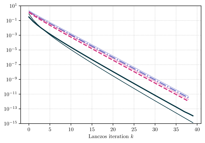
(a) Error bounds for $f(x)=\log(x)$ using a Pac-Man contour as described in Example 6.2. $\mathbf{A}=\mathbf{X}\mathbf{X}^{\textup{{T}}}$, where the entries of $\mathbf{X}\in\mathbb{R}^{n,2n}$ are independent Gaussians with mean zero variance $1/2n$ where $n=3000$. Legend: A priori bounds obtained by using Eq. 18 with $S_{0}=S_{i}=\mathcal{I}(\mathbf{A})$ () and $S_{0}=S_{i}=\tilde{\mathcal{I}}(\mathbf{A})$ (). A posteriori bounds obtained by using Eq. 18 with $S_{0}=\mathcal{I}(\mathbf{A})$, $S_{i}=\{\lambda_{i}(\mathbf{T}_{k})\}$ () and $S_{0}=\tilde{\mathcal{I}}(\mathbf{A})$, $S_{i}=\{\lambda_{i}(\mathbf{T}_{k})\}$ ().

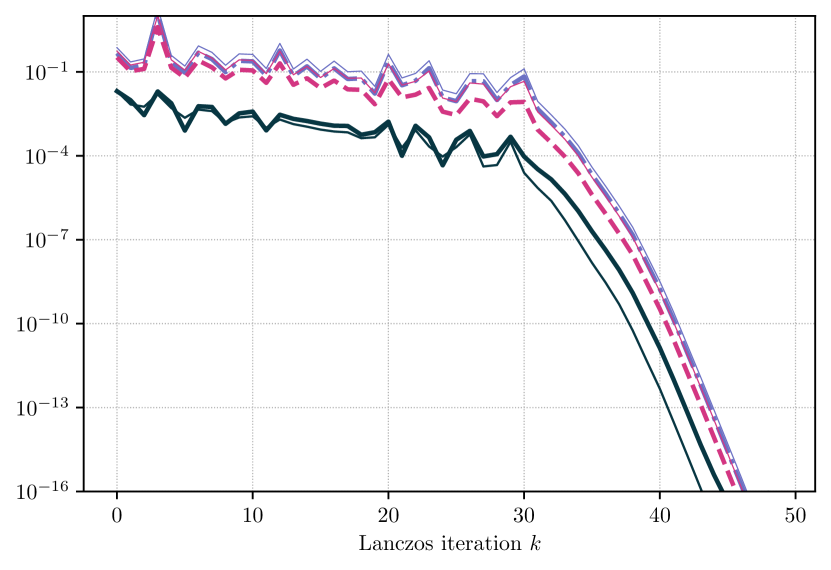
(b) Error bounds for $f(x)=\operatorname{step}(x-a)$ with double circle contour as described in Example 6.3. $\mathbf{A}$ is the covariance matrix of the MNIST training data [41]. Legend: A priori bounds obtained by using Eq. 18 with $S_{0}=S_{i}=\mathcal{I}_{w}(\mathbf{A})$ () and $S_{0}=S_{i}=\tilde{\mathcal{I}}_{w}(\mathbf{A})$ (). A posteriori bounds obtained by using Eq. 18 with $S_{0}=\mathcal{I}_{w}(\mathbf{A})$, $S_{i}=\{\lambda_{i}(\mathbf{T}_{k})\}$ () and $S_{0}=\tilde{\mathcal{I}}_{w}(\mathbf{A})$, $S_{i}=\{\lambda_{i}(\mathbf{T}_{k})\}$ ().

Figure 7: Lanczos-FA quadratic form errors. Legend: $|\mathbf{b}^{\textup{{H}}}f(\mathbf{A})\mathbf{b}-\mathbf{b}^{\textup{{H}}}\textup{{lan}}_{k}(f)|$ (). For reference we also show $\|f(\mathbf{A})\mathbf{b}-\textup{{lan}}_{k}(f)\|_{2}^{2}$ (). Note that this is the square of the 2-norm of the Lanczos-FA error.

In the case that the contour $\Gamma$ does not pass through $\mathcal{I}(\mathbf{A})$, the bound of Eq. 18 is essentially as easy to compute as that of Theorem 2.8. However, if the contour passes through $\mathcal{I}(\mathbf{A})$ at $w$, to ensure that $S_{0}$ does not contain points in the contour, it must be chosen as a set other than $\mathcal{I}(\mathbf{A})$. This set must contain all of $\mathbf{A}$’s eigenvalues and we must bound its distance to the contour (in particular, to $w$).

Example 6.2.

Suppose $\mathbf{A}$ is positive definite and $f(x)=\log(x)$. We use Eq. 18 to obtain a bound for the quadratic form error $|\mathbf{b}^{\textup{{H}}}f(\mathbf{A})\mathbf{b}-\mathbf{b}^{\textup{{H}}}\textup{{lan}}_{k}(f)|$. A priori bounds are obtained with $S_{0},S_{i}=\mathcal{I}(\mathbf{A})$ while a posteriori bounds are obtained with $S_{0}=\mathcal{I}(\mathbf{A})$ and $S_{i}=\{\lambda_{i}(\mathbf{T}_{k})\}$. In both cases, we take $\Gamma$ as the Pac-Man contour centered at 0 with $r=\lambda_{\text{min}}(\mathbf{A})/100$ to avoid the singularity $\log(0)=-\infty$. The resulting bounds are shown in the left panel of Fig. 7.

As in Example 4.1, we also consider the cases where we use an estimate $\tilde{\mathcal{I}}(\mathbf{A})$ for $\mathcal{I}(\mathbf{A})$ to study the sensitivity of our bounds to $S_{i}$. For these tests we use a Pac-Man contour with $r=\lambda_{\text{min}}(\mathbf{A})/200$.

Example 6.3.

Let $f(x)=\operatorname{step}(x-a)$ for $a\in\mathcal{I}(\mathbf{A})$, and set $w=a$. Similarly to the previous example we use Eq. 18 to obtain a bound for the quadratic form error $|\mathbf{b}^{\textup{{H}}}f(\mathbf{A})\mathbf{b}-\mathbf{b}^{\textup{{H}}}\textup{{lan}}_{k}(f)|$. However, we must have $S_{i}$ avoid where $\Gamma$ crosses the real axis.

Suppose $\lambda_{\text{max}}^{\text{l},w}(\mathbf{A})$ and $\lambda_{\text{min}}^{\text{r},w}(\mathbf{A})$ are consecutive eigenvalues of $\mathbf{A}$ so that $\lambda_{\text{max}}^{\text{l},w}(\mathbf{A})<w<\lambda_{\text{min}}^{\text{r},w}(\mathbf{A})$. Then we can define

$$\mathcal{I}_{w}(\mathbf{A}):=[\lambda_{\text{min}}(\mathbf{A}),\lambda_{\text{max}}^{\text{l},w}(\mathbf{A})]\cup[\lambda_{\text{min}}^{\text{r},w}(\mathbf{A}),\lambda_{\text{max}}(\mathbf{A})].$$

In this case, $\|h_{z}\|_{\mathcal{I}_{w}(\mathbf{A})}=\max\{\|h_{z}\|_{[\lambda_{\text{min}},\lambda_{\text{max}}^{\text{l},w}]},\|h_{z}\|_{[\lambda_{\text{min}}^{\text{r},w},\lambda_{\text{max}}]})\}$ can be computed using Lemma 6.1.

We can then apply Eq. 18 to obtain a bound for the quadratic form error $|\mathbf{b}^{\textup{{H}}}f(\mathbf{A})\mathbf{b}-\mathbf{b}^{\textup{{H}}}\textup{{lan}}_{k}(f)|$. A priori bounds are obtained with $S_{0},S_{i}=\mathcal{I}_{w}(\mathbf{A})$ while a posteriori bounds are obtained with $S_{0}=\mathcal{I}_{w}(\mathbf{A})$ and $S_{i}=\{\lambda_{i}(\mathbf{T}_{k})\}$. This is shown in the right panel of Fig. 7. Of course, in practice it is unlikely that $\lambda_{\text{min}}^{\text{l},w}(\mathbf{A})$ and $\lambda_{\text{max}}^{\text{r},w}(\mathbf{A})$ are known. The distance to $w$ of course can be estimated by estimating the smallest eigenvalue of $(\mathbf{A}-w\mathbf{I})^{2}$, perhaps via Lanczos. However, it can be expected to be more difficult than estimating $\lambda_{\text{min}}(\mathbf{A})$ and $\lambda_{\text{max}}(\mathbf{A})$. Thus, we also show the effect of approximating $\lambda_{\text{max}}^{\text{l},w}(\mathbf{A})$ and $\lambda_{\text{min}}^{\text{l},w}(\mathbf{A})$. Specifically, we compute $\|h_{w,z}\|_{\tilde{\mathcal{I}}_{w}(\mathbf{A})}$ where

$$\tilde{\mathcal{I}}_{w}(\mathbf{A})=[\lambda_{\text{min}}/2,w-\gamma]\cup[w+\gamma,1.5\lambda_{\max}])$$

for $\gamma=\min_{\lambda\in\Lambda(\mathbf{A})}|\lambda-w|/100$.

7 Conclusion and outlook

In this paper we give a simple approach to generate error bounds for Lanczos-FA used to approximate $f(\mathbf{A})\mathbf{b}$ when $f(x)$ is piecewise analytic. Our framework can be used both a priori and a posteriori, and the bounds, to close degree, hold in finite precision. While outside the scope of this paper, the same general approach is applicable to non-Hermitian matrices computed using an Arnoldi factorization.

8 Acknowledgments

The authors thank Thomas Trogdon for suggestions in early stages.

Appendix A Error bounds for Lanczos on linear systems

Our analysis reduces understanding the Lanczos-FA error for a function $f$ to understanding $\|\textup{{err}}_{k}(w)\|$, the error of Lanczos-FA used to solve the system $(\mathbf{A}-w\mathbf{I})\mathbf{x}=\mathbf{b}$. We review several bounds for this task. Without loss of generality, we assume $w=0$, as the $w\mathbf{I}$ term can be incorperated directly into $\mathbf{A}$.

In the case that $\mathbf{A}$ is positive (or negative) definite, Lanczos-FA with $f(x)=1/x$ is equivalent to the conjugate gradient algorithm (CG) [31]. Therefore, it inherits CG’s well known property of returning an optimal solution in the $\mathbf{A}$-norm (or $-\mathbf{A}$-norm if $\mathbf{A}$ is negative definite). That is,

$$\|\textup{{err}}_{k}\|_{\mathbf{A}}=\min_{\mathbf{y}\in\mathcal{K}_{k}(\mathbf{A},\mathbf{b})}\|\mathbf{A}^{-1}\mathbf{b}-\mathbf{y}\|_{\mathbf{A}}=\min_{\begin{subarray}{c}\deg p\leq k\\ p(0)=1\end{subarray}}\|p(\mathbf{A})\mathbf{A}^{-1}\mathbf{b}\|_{\mathbf{A}}.$$

From this optimality, we obtain the following (well known) bounds for positive definite $\mathbf{A}$

$$\frac{\|\textup{{err}}_{k}\|_{\mathbf{A}}}{\|\textup{{err}}_{0}\|_{\mathbf{A}}}\leq\min_{\begin{subarray}{c}\deg p\leq k\\ p(0)=1\end{subarray}}\max_{\lambda\in\Lambda(\mathbf{A})}|p(\lambda)|\leq 2\left(\frac{\sqrt{\kappa(\mathbf{A})}-1}{\sqrt{\kappa(\mathbf{A})}+1}\right)^{k}\leq 2\exp\left(-\frac{2k}{\sqrt{\kappa(\mathbf{A})}}\right)$$

where the final bound follows from the fact that $(x-1)/(x+1)\leq\exp(-2/x)$ for all $x\geq 1$. The minimax bound, based on the eigenvalues of $\mathbf{A}$, is tight in the sense that for each $k$ there exists $\mathbf{b}$ (dependent on $\mathbf{A}$ and $k$) so that $\textup{{lan}}_{k}(f,\mathbf{A},\mathbf{b})$ attains the bound [24]. The final inequality implies that Lanczos-FA requires $k\leq\frac{1}{2}\sqrt{\kappa(\mathbf{A})}\log(2/\epsilon)$ iterations to ensure $\|\textup{{err}}_{k}\|_{\mathbf{A}}/\|\textup{{err}}_{0}\|_{\mathbf{A}}\leq\epsilon$.

From the result above, it is also straightforward to derive a bound that is more directly comparable to Eq. 2 and Eq. 3. Specifically, for $f(x)=1/x$, [45] shows:

$$\|\textup{{err}}_{k}\|_{2}=\|f(\mathbf{A})\mathbf{b}-\textup{{lan}}_{k}(f)\|_{2} \leq\sqrt{\kappa(\mathbf{A})}\|\mathbf{b}\|_{2}\cdot\min_{\deg p<k}\|f-p\|_{\Lambda(\mathbf{A})}.$$

Beside the leading constant $\sqrt{\kappa(\mathbf{A})}$, this bound is strictly stronger than Eq. 2 because it only depends on the eigenvalues of $\mathbf{A}$, and not those of $\mathbf{T}_{k}$. As a result, it is also strictly stronger than the uniform approximation bound of Eq. 3.

If $\mathbf{A}$ is indefinite, we can obtain error bounds by relating the Lanczos-FA approximation to MINRES. For these bounds, we need the following theorem from [8] which compares the 2-norm of the residual in the Lanczos approximation to the solution of a Hermitian linear system to that of the MINRES algorithm. MINRES, by definition, minimizes the 2-norm of the residual over all approximations from the Krylov subspace.

Theorem A.1.

Let $\mathbf{A}$ be a nonsingular Hermitian matrix and define $\mathbf{r}_{k}^{M}$ as the MINRES residual at step $k$; i.e.

$$\mathbf{r}_{k}^{M}:=\mathbf{b}-\mathbf{A}\hat{\mathbf{y}}, \hat{\mathbf{y}}=\operatorname*{argmin}_{\mathbf{y}\in\mathcal{K}_{k}(\mathbf{A},\mathbf{b})}\|\mathbf{b}-\mathbf{A}\mathbf{y}\|_{2}.$$

Then, assuming that the initial residuals in the two procedures are the same,

$$\frac{\|\textup{{res}}_{k}\|_{2}}{\|\textup{{res}}_{0}\|_{2}}=\frac{\|\mathbf{r}_{k}^{M}\|_{2}/\|\mathbf{r}_{0}^{M}\|_{2}}{\sqrt{1-\left(\|\mathbf{r}_{k}^{M}\|_{2}/\|\mathbf{r}_{k-1}^{M}\|_{2}\right)^{2}}}.$$

Therefore, if MINRES makes good progress at step $k$ (i.e. $\|\mathbf{r}_{k}^{M}\|_{2}/\|\mathbf{r}_{k-1}^{M}\|_{2}$ is small), then Theorem A.1 implies $\|\textup{{res}}_{k}\|_{2}/\|\textup{{res}}_{0}\|_{2}\approx\|\mathbf{r}_{k}^{M}\|_{2}/\|\mathbf{r}_{0}^{M}\|_{2}$. Thus, since MINRES converges at a linear rate, there will be iterations in which Lanczos-FA has nearly as good a residual norm as MINRES. This is made precise by the following result.

Corollary A.2.

Suppose $\Lambda(\mathbf{A})\subset[a,b]\cup[c,d]$, where $a<b<0<c<d$ with $b-a=d-c$, and define $\gamma=\sqrt{|ad|/|bc|}$. Then, for any $\epsilon<\gamma/4$ there exsits $k\leq 2\gamma\log(\sqrt{2}\gamma/\epsilon)$ so that $\|\textup{{res}}_{k}\|_{2}/\|\textup{{res}}_{0}\|_{2}<\epsilon$.

Proof A.3.

If the eigenvalues of $\mathbf{A}$ lie in $[a,b]\cup[c,d]$, where $a<b<0<c<d$ and $b-a=d-c$, then as in [27, Section 3.1], the optimality of MINRES implies

$$\frac{\|\mathbf{r}_{j}^{M}\|_{2}}{\|\mathbf{r}_{0}^{M}\|_{2}}\leq 2\left(\frac{\sqrt{|ad|/|bc|}-1}{\sqrt{|ad|/|bc|}+1}\right)^{\lfloor j/2\rfloor}\leq 2\exp\left(-\frac{2\lfloor j/2\rfloor}{\sqrt{|ad|/|bc|}}\right).$$

For notational convenience set $\tau=2\epsilon/\gamma$ and define $k^{\prime}$ to be the first iteration where $\|r_{k^{\prime}}^{M}\|_{2}/\|r_{0}\|_{2}<\tau/2$ and $k^{\prime\prime}$ to be the first iteration where $\|r_{k^{\prime\prime}}^{M}\|_{2}/\|r_{0}\|_{2}<\tau^{2}/4$. Note that $k^{\prime\prime}\leq\gamma\log(2/(\tau^{2}/4))=2\gamma\log(2\sqrt{2}/\tau)$.

First, suppose $\|r_{k^{\prime}}\|_{2}/\|r_{0}\|_{2}\leq\tau/4$. Then, since $\|r_{k^{\prime}-1}\|_{2}/\|r_{0}\|_{2}>\tau/2$, using Theorem A.1,

$$\frac{\|\textup{{res}}_{k}\|_{2}}{\|\textup{{res}}_{0}\|_{2}}=\frac{\|\mathbf{r}_{k^{\prime}}^{M}\|_{2}/\|\mathbf{r}_{0}^{M}\|_{2}}{\sqrt{1-\left(\|\mathbf{r}_{k^{\prime}}^{M}\|_{2}/\|\mathbf{r}_{k^{\prime}-1}^{M}\|_{2}\right)^{2}}}\leq\frac{\tau/4}{\sqrt{1-((\tau/4)/(\tau/2))^{2}}}=\frac{\tau}{2\sqrt{3}}\leq\epsilon.$$

Next, suppose that $\|r_{k^{\prime}}\|_{2}/\|r_{0}\|_{2}>\tau/4$. Let $\ell=k^{\prime\prime}-k$ and note that there must exist an iteration $k\in(k^{\prime},k^{\prime\prime}]$ so that

$$\frac{\|\mathbf{r}_{k}^{M}\|_{2}}{\|\mathbf{r}_{k-1}^{M}\|_{2}}=\frac{\|\mathbf{r}_{k}^{M}\|_{2}/\|\mathbf{r}_{0}^{M}\|_{2}}{\|\mathbf{r}_{k-1}^{M}\|_{2}/\|\mathbf{r}_{0}^{M}\|_{2}}\leq\left(\frac{\tau^{2}/4}{\tau/4}\right)^{1/\ell}.$$

Now note that

$$\frac{1}{\sqrt{1-\left(\left(\frac{\tau^{2}/4}{\tau/4}\right)^{1/\ell}\right)^{2}}}=\frac{1}{\sqrt{1-\tau^{2/\ell}}}$$

and that $\ell\leq k^{\prime\prime}-1\leq 2\gamma\log(2\sqrt{2}/\tau)$ so

$$\frac{1}{\sqrt{1-\tau^{2/\ell}}}\leq\frac{1}{\sqrt{1-\tau^{1/(\gamma\log(2\sqrt{2}/\tau))}}}=\frac{1}{\sqrt{1-\left(\tau^{1/\log(2\sqrt{2}/\tau)}\right)^{1/\gamma}}}$$

If $\tau\in[0,1/2]$ then $\tau^{1/\log(2\sqrt{2}/\tau)}\leq\exp(-2/5)<3/4$ so noting that $\gamma\geq 1$ we can apply Lemma A.4 to obtain

$$\frac{1}{\sqrt{1-\left(\tau^{1/\log(2\sqrt{2}/\tau)}\right)^{1/\gamma}}}\leq 2\gamma.$$

Combining this with Theorem A.1 gives,

$$\frac{\|\textup{{res}}_{k}\|_{2}}{\|\textup{{res}}_{0}\|_{2}}=\frac{\|\mathbf{r}_{k^{\prime}}^{M}\|_{2}/\|\mathbf{r}_{0}^{M}\|_{2}}{\sqrt{1-\left(\|\mathbf{r}_{k^{\prime}}^{M}\|_{2}/\|\mathbf{r}_{k^{\prime}-1}^{M}\|_{2}\right)^{2}}}\leq\frac{\tau/4}{\sqrt{1-\left(\left(\frac{\tau^{2}/4}{\tau/4}\right)^{1/\ell}\right)^{2}}}\leq\frac{\tau\gamma}{2}=\epsilon.$$

Lemma A.4.

For all $x\in[0,3/4]$ and $y\in[0,1]$,

$$\frac{1}{\sqrt{1-x^{y}}}\leq\frac{2}{y}.$$

Proof A.5.

Consider the function

$$g(x,y)=\frac{y}{2\sqrt{1-x^{y}}}.$$

For any $y\in[0,1]$, $g(x,y)$ is non-decreasing in $x$, so it suffices to set $x=3/4$. Thus, define

$$f(y)=\log(g(3/4,y))=\log\left(\frac{y}{2\sqrt{1-(3/4)^{y}}}\right)$$

which has derivative

$$f^{\prime}(y)=\frac{1}{y}-\frac{\log(4/3)}{2((4/3)^{y}-1)}.$$

? Note that $(4/3)^{y}-1\geq\log(4/3)y$ for all $y\geq 0$ so

$$\frac{\log(4/3)}{2((4/3)^{y}-1)}\leq\frac{\log(4/3)}{2\log(4/3)y}=\frac{1}{2y}.$$

Therefore $f^{\prime}(y)\geq 1/(2y)\geq 0$, so $f(y)$ is non-decreasing. Since $\log$ is increasing this implies that $g(3/4,y)$ is a non-decreasing function of $y$ on $[0,1]$ and therefore bounded above by $g(3/4,1)=1$. Thus, $g(x,y)\leq 1$ for all $x\in[0,3/4]$ and $y\in[0,1]$ and the result follows.

So far we have discussed a priori bounds, but there are a range of a posteriori bounds as well. For instance, a simple a posteriori bound is obtained using the fact that $\|\textup{{err}}_{k}\|_{\mathbf{A}^{2}}=\|\textup{{res}}_{k}\|_{2}$, which holds even when $\mathbf{A}$ is indefinite. Using the similarity of matrix norms, bounds for $\|\textup{{err}}_{k}\|$ when $\|\cdot\|$ is any norm induced by a matrix with the same eigenvectors as $\mathbf{A}$ can then be obtained.

When $\mathbf{A}$ is positive (or negative) definite, a range of more refined error bounds and estimates for the $\mathbf{A}$-norm and 2-norm have been considered. These bounds obtain error estimates for CG at step $k$ by running Lanczos (or CG) for an extra $d$ iterations. The information from this larger Krylov subspace $\mathcal{K}_{k+d}(\mathbf{A},\mathbf{b})$ is then used to estimate the error at step $k$. Typically $d$ can be taken as a small constant, say $d=5$, so the extra work required to obtain these bounds is not too large. We refer to [54, 44, 15, 42] and the references within for more details.

References

- [1] N. I. Aheizer and N. Kemmer, The classical moment problem and some related questions in analysis, Oliver & Boyd Edinburgh, 1965.
- [2] Z. Allen-Zhu and Y. Li, Faster principal component regression and stable matrix Chebyshev approximation, in Proceedings of the 34th International Conference on Machine Learning, D. Precup and Y. W. Teh, eds., vol. 70 of Proceedings of Machine Learning Research, International Convention Centre, Sydney, Australia, 06–11 Aug 2017, PMLR, pp. 107–115.
- [3] C. Berg, Stieltjes-Pick-Bernstein-Schoenberg and their connection to complete monotonicity, 2007. http://citeseerx.ist.psu.edu/viewdoc/versions?doi=10.1.1.142.3872.
- [4] A. Boriçi, On the Neuberger overlap operator, Physics Letters B, 453 (1999), pp. 46–53.
- [5] , Computational methods for UV-suppressed fermions, Journal of Computational Physics, 189 (2003), pp. 454–462.
- [6] V. Braverman, A. Krishnan, and C. Musco, Linear and sublinear time spectral density estimation, 2021. arXiv cs.DS 2104.03461.
- [7] T. Chen, T. Trogdon, and S. Ubaru, Analysis of stochastic Lanczos quadrature for spectrum approximation, in Proceedings of the 37th International Conference on Machine Learning, Proceedings of Machine Learning Research, PMLR, 2021.
- [8] J. Cullum and A. Greenbaum, Relations between Galerkin and norm-minimizing iterative methods for solving linear systems, SIAM Journal on Matrix Analysis and Applications, 17 (1996), pp. 223–247.
- [9] P. I. Davies and N. J. Higham, Computing for matrix functions , in QCD and numerical analysis III, Springer, 2005, pp. 15–24.
- [10] E. Di Napoli, E. Polizzi, and Y. Saad, Efficient estimation of eigenvalue counts in an interval, Numerical Linear Algebra with Applications, 23 (2016), pp. 674–692.
- [11] V. Druskin, A. Greenbaum, and L. Knizhnerman, Using nonorthogonal Lanczos vectors in the computation of matrix functions, SIAM Journal on Scientific Computing, 19 (1998), pp. 38–54.
- [12] V. Druskin and L. Knizhnerman, Two polynomial methods of calculating functions of symmetric matrices, USSR Computational Mathematics and Mathematical Physics, 29 (1989), pp. 112–121.
- [13] , Error bounds in the simple Lanczos procedure for computing functions of symmetric matrices and eigenvalues, Comput. Math. Math. Phys., 31 (1992), p. 20–30.
- [14] V. Druskin and L. Knizhnerman, Krylov subspace approximation of eigenpairs and matrix functions in exact and computer arithmetic, Numerical Linear Algebra with Applications, 2 (1995), pp. 205–217.
- [15] R. Estrin, D. Orban, and M. Saunders, Euclidean-norm error bounds for SYMMLQ and CG, SIAM Journal on Matrix Analysis and Applications, 40 (2019), pp. 235–253.
- [16] A. Frommer, S. Güttel, and M. Schweitzer, Convergence of restarted Krylov subspace methods for Stieltjes functions of matrices, SIAM Journal on Matrix Analysis and Applications, 35 (2014), pp. 1602–1624.
- [17] , Efficient and stable Arnoldi restarts for matrix functions based on quadrature, SIAM Journal on Matrix Analysis and Applications, 35 (2014), pp. 661–683.
- [18] A. Frommer, K. Kahl, T. Lippert, and H. Rittich, 2-norm error bounds and estimates for Lanczos approximations to linear systems and rational matrix functions, SIAM Journal on Matrix Analysis and Applications, 34 (2013), pp. 1046–1065.
- [19] A. Frommer and M. Schweitzer, Error bounds and estimates for Krylov subspace approximations of Stieltjes matrix functions, BIT Numerical Mathematics, 56 (2015), pp. 865–892.
- [20] A. Frommer and V. Simoncini, Stopping criteria for rational matrix functions of Hermitian and symmetric matrices, SIAM Journal on Scientific Computing, 30 (2008), pp. 1387–1412.
- [21] A. Frommer and V. Simoncini, Error bounds for Lanczos approximations of rational functions of matrices, in Numerical Validation in Current Hardware Architectures, Berlin, Heidelberg, 2009, Springer Berlin Heidelberg, pp. 203–216.
- [22] R. Frostig, C. Musco, C. Musco, and A. Sidford, Principal component projection without principal component analysis, in International Conference on Machine Learning, 2016, pp. 2349–2357.
- [23] G. H. Golub and G. Meurant, Matrices, moments and quadrature with applications, vol. 30, Princeton University Press, 2009.
- [24] A. Greenbaum, Comparison of splittings used with the conjugate gradient algorithm, Numerische Mathematik, 33 (1979), pp. 181–193.
- [25] , Behavior of slightly perturbed Lanczos and conjugate-gradient recurrences, Linear Algebra and its Applications, 113 (1989), pp. 7 – 63.
- [26] , Estimating the attainable accuracy of recursively computed residual methods, SIAM Journal on Matrix Analysis and Applications, 18 (1997), pp. 535–551.
- [27] , Iterative Methods for Solving Linear Systems, Society for Industrial and Applied Mathematics, Philadelphia, PA, USA, 1997.
- [28] M. Gu and S. C. Eisenstat, A divide-and-conquer algorithm for the symmetric tridiagonal eigenproblem, SIAM Journal on Matrix Analysis and Applications, 16 (1995), pp. 172–191.
- [29] S. Güttel and M. Schweitzer, A comparison of limited-memory Krylov methods for Stieltjes functions of Hermitian matrices, SIAM Journal on Matrix Analysis and Applications, 42 (2021), pp. 83–107.
- [30] N. Hale, N. J. Higham, and L. N. Trefethen, Computing , and related matrix functions by contour integrals, SIAM Journal on Numerical Analysis, 46 (2008), pp. 2505–2523.
- [31] M. R. Hestenes and E. Stiefel, Methods of conjugate gradients for solving linear systems, vol. 49, NBS Washington, DC, 1952.
- [32] N. J. Higham, Functions of Matrices, Society for Industrial and Applied Mathematics, 2008.
- [33] M. Hochbruck and C. Lubich, On Krylov subspace approximations to the matrix exponential operator, SIAM Journal on Numerical Analysis, 34 (1997), pp. 1911–1925.
- [34] M. Hochbruck, C. Lubich, and H. Selhofer, Exponential integrators for large systems of differential equations, SIAM Journal on Scientific Computing, 19 (1998), pp. 1552–1574.
- [35] M. D. Ilic, I. W. Turner, and D. P. Simpson, A restarted Lanczos approximation to functions of a symmetric matrix, IMA Journal of Numerical Analysis, 30 (2009), pp. 1044–1061.
- [36] T. Jawecki, A study of defect-based error estimates for the Krylov approximation of -functions, Numerical Algorithms, (2021).
- [37] T. Jawecki, W. Auzinger, and O. Koch, Computable upper error bounds for Krylov approximations to matrix exponentials and associated -functions, BIT Numerical Mathematics, 60 (2019), pp. 157–197.
- [38] Z. Jia and H. Lv, A posteriori error estimates of Krylov subspace approximations to matrix functions, 69 (2014), pp. 1–28.
- [39] Y. Jin and A. Sidford, Principal component projection and regression in nearly linear time through asymmetric SVRG, in Advances in Neural Information Processing Systems 32, H. Wallach, H. Larochelle, A. Beygelzimer, F. d Alché-Buc, E. Fox, and R. Garnett, eds., Curran Associates, Inc., 2019, pp. 3868–3878.
- [40] J. Kuczyński and H. Woźniakowski, Estimating the largest eigenvalue by the power and Lanczos algorithms with a random start, SIAM Journal on Matrix Analysis and Applications, 13 (1992), pp. 1094–1122.
- [41] Y. LeCun, C. Cortes, and C. Burges, MNIST handwritten digit database, (2010).
- [42] G. Meurant, J. Papež, and P. Tichý, Accurate error estimation in CG, Numerical Algorithms, (2021).
- [43] G. Meurant and Z. Strakoš, The Lanczos and conjugate gradient algorithms in finite precision arithmetic, Acta Numerica, 15 (2006), pp. 471–542.
- [44] G. Meurant and P. Tichý, Approximating the extreme Ritz values and upper bounds for the -norm of the error in CG, Numerical Algorithms, 82 (2018), pp. 937–968.
- [45] C. Musco, C. Musco, and A. Sidford, Stability of the Lanczos method for matrix function approximation, in Proceedings of the Twenty-Ninth Annual ACM-SIAM Symposium on Discrete Algorithms, SODA ’18, USA, 2018, Society for Industrial and Applied Mathematics, p. 1605–1624.
- [46] C. C. Paige, The computation of eigenvalues and eigenvectors of very large sparse matrices., PhD thesis, University of London, 1971.
- [47] , Error Analysis of the Lanczos Algorithm for Tridiagonalizing a Symmetric Matrix, IMA Journal of Applied Mathematics, 18 (1976), pp. 341–349.
- [48] , Accuracy and effectiveness of the Lanczos algorithm for the symmetric eigenproblem, Linear Algebra and its Applications, 34 (1980), pp. 235 – 258.
- [49] C. C. Paige, Accuracy of the lanczos process for the eigenproblem and solution of equations, SIAM Journal on Matrix Analysis and Applications, 40 (2019), pp. 1371–1398.
- [50] B. N. Parlett, H. Simon, and L. M. Stringer, On estimating the largest eigenvalue with the Lanczos algorithm, Mathematics of Computation, 38 (1982), pp. 153–153.
- [51] G. Pleiss, M. Jankowiak, D. Eriksson, A. Damle, and J. Gardner, Fast matrix square roots with applications to Gaussian processes and Bayesian optimization, in Advances in Neural Information Processing Systems, H. Larochelle, M. Ranzato, R. Hadsell, M. F. Balcan, and H. Lin, eds., vol. 33, Curran Associates, Inc., 2020, pp. 22268–22281.
- [52] Y. Saad, Analysis of some Krylov subspace approximations to the matrix exponential operator, SIAM Journal on Numerical Analysis, 29 (1992), pp. 209–228.
- [53] Z. Strakos and A. Greenbaum, Open questions in the convergence analysis of the Lanczos process for the real symmetric eigenvalue problem, University of Minnesota, 1992.
- [54] Z. Strakoš and P. Tichỳ, On error estimation in the conjugate gradient method and why it works in finite precision computations., ETNA. Electronic Transactions on Numerical Analysis [electronic only], 13 (2002), pp. 56–80.
- [55] L. N. Trefethen and J. A. C. Weideman, The exponentially convergent trapezoidal rule, SIAM Review, 56 (2014), pp. 385–458.
- [56] S. Ubaru, J. Chen, and Y. Saad, Fast estimation of via stochastic Lanczos quadrature, SIAM Journal on Matrix Analysis and Applications, 38 (2017), pp. 1075–1099.
- [57] J. van den Eshof, A. Frommer, T. Lippert, K. Schilling, and H. van der Vorst, Numerical methods for the QCDd overlap operator. I. Sign-function and error bounds, Computer Physics Communications, 146 (2002), pp. 203 – 224.