A Distance-based Separability Measure for Internal Cluster Validation
Abstract
To evaluate clustering results is a significant part of cluster analysis. Since there are no true class labels for clustering in typical unsupervised learning, many internal cluster validity indices (CVIs), which use predicted labels and data, have been created. Without true labels, to design an effective CVI is as difficult as to create a clustering method. And it is crucial to have more CVIs because there are no universal CVIs that can be used to measure all datasets and no specific methods of selecting a proper CVI for clusters without true labels. Therefore, to apply a variety of CVIs to evaluate clustering results is necessary. In this paper, we propose a novel internal CVI – the Distance-based Separability Index (DSI), based on a data separability measure. We compared the DSI with eight internal CVIs including studies from early Dunn (1974) to most recent CVDD (2019) and an external CVI as ground truth, by using clustering results of five clustering algorithms on 12 real and 97 synthetic datasets. Results show DSI is an effective, unique, and competitive CVI to other compared CVIs. We also summarized the general process to evaluate CVIs and created the rank-difference metric for comparison of CVIs’ results. The code can be found in author’s website linked up with the ORCID: https://orcid.org/0000-0002-3779-9368.
keywords:
cluster validity; cluster validity index evaluation; clustering analysis; separability measure; distance-based separability index; sequence comparison.1 Introduction
Cluster analysis is an important unsupervised learning method in machine learning. The clustering algorithms divide a dataset into clusters [Jain1999Data] based on the distribution structure of the data, without any prior knowledge. Clustering is widely studied and used in many fields, such as data mining, pattern recognition, object detection, image segmentation, bioinformatics, and data compression [Roiger2017Data, Wen2019shape-based, Guan2018Application, Dhanachandra2017survey, Karim2020Deep, Marchetti2018Spatial]. The shortage of labels for training is a big problem in some machine learning applications, such as medical image analysis, and applications of big data [Nasraoui2019Clustering] because labeling is expensive [Hoo-Chang2016Deep]. Since unsupervised machine learning does not use labels for training, to apply cluster analysis can avoid the problem.
In general, the main methods of cluster analysis can be categorized into centroid-based (e.g., k-means), distribution-based (e.g., EM algorithm [Byrne2017EM]), density-based (e.g., DBSCAN [Ester1996density-based]), hierarchical (e.g., Ward linkage [Ward_Jr1963Hierarchical]), and spectral clustering [Von_Luxburg2007tutorial]. None of the clustering methods, however, is able to perform well with all kinds of datasets [Kleinberg2003Impossibility, Von_Luxburg2012Clustering:]. That is, a clustering method that performs well with some types of datasets would perform poorly with some others. For this reason, various clustering methods have been applied to datasets. Consequently, effective clustering validations (measures of clustering quality) are required to evaluate which clustering method performs well for a dataset [Ben-David2009Measures, Adolfsson2019To]. And, clustering validations are also used to tune the parameters of clustering algorithms.
There are two categories of clustering validations: internal and external validations. External validations use the truth-labels of classes and predicted labels, and internal validations use predicted labels and data. Since external validations require true labels and there are no true class labels in unsupervised learning tasks, we can employ only the internal validations in cluster analysis [Liu2013Understanding]. In fact, to evaluate clustering results by internal validations has the same difficulty as to do clustering itself because measures have no more information than the clustering methods [Pfitzner2008Characterization]. Therefore, the difficulty of designing an internal Cluster Validity Index (CVI) is like creating a clustering algorithm. The different part is that a clustering algorithm can update clustering results by a value (loss) from the optimizing function but the CVI provides only a value for clusters evaluation.
1.1 Related works
Various CVIs have been created for the clustering of many types of datasets [Desgraupes2017Clustering]. By methods of calculation [Hu2019Internal], the internal CVIs are based on two categories of representatives: center and non-center. Center-based internal CVIs use descriptors of clusters. For example, the Davies–Bouldin index (DB) [Davies1979Cluster] uses cluster diameters and the distance between cluster centroids. Non-center internal CVIs use descriptors of data points. For example, the Dunn index [Dunn1974Well-Separated] considers the minimum and maximum distances between two data points.
Besides the DB and Dunn indexes, in this paper, some other typical internal CVIs are selected for comparison. The Calinski-Harabasz index (CH) [Calinski1974dendrite] and Silhouette coefficient (Sil) [Rousseeuw1987Silhouettes:] are two traditional internal CVIs. In recently developed internal CVIs, the I index [Maulik2002Performance], WB index [Zhao2014WB-index:], Clustering Validation index based on Nearest Neighbors (CVNN) [Liu2013Understanding], and Cluster Validity index based on Density-involved Distance (CVDD) [Hu2019Internal] are selected. Eight typical internal CVIs, which range from early studies (Dunn, 1974) to the most recent studies (CVDD, 2019), are selected to compare with our proposed CVI.
In addition, an external CVI - the Adjusted Rand Index (ARI) [Santos2009On] is selected as the ground truth for comparison because external validations use the true class labels and predicted labels. Unless otherwise indicated, the “CVIs” that appear hereafter mean internal CVIs and the only external CVI is named “ARI”.
2 Distance-based Separability Measure
Since the goal of clustering is to separate a dataset into clusters, in the macro-perspective, how well a dataset has been separated could be indicated via the separability of clusters. In a dataset, data points are assigned class labels by the clustering algorithm. The most difficult situation for separation of the dataset occurs when all labels are randomly assigned and the data points of different classes will have the same distribution (distributions have the same shape, position, and support, i.e., the same probability density function). To analyze the distributions of different-class data, we propose the Distance-based Separability Index (DSI) 333More studies about the DSI will appear in other forthcoming publications, which can be found in author’s website linked up with the ORCID: https://orcid.org/0000-0002-3779-9368..
Suppose a dataset contains two classes , and have , data points, respectively, we can define:
Definition 2.1.
The Intra-Class Distance (ICD) set is a set of distances between any two points in the same class. e.g., for class , its ICD set :
Remark 2.2.
The metric for distance is Euclidean . Given , then .
Definition 2.3.
The Between-Class Distance (BCD) set is the set of distances between any two points from different classes. e.g., for class and , their BCD set :
Remark 2.4.
Given , then .
Then, the Theorem 2.5 shows how the ICD and BCD sets are related to the distributions of data:
Theorem 2.5.
When , if and only if the two classes and have the same distribution, the distributions of the ICD and BCD sets are identical.
The full proof of Theorem 2.5 is shown in LABEL:sec:proof. Here we provide an informal explanation: points in and having the same distribution and covering the same region can be considered to have been sampled from one distribution . Hence, both ICDs of and , and BCDs between and are actually ICDs of . Consequently, the distributions of ICDs and BCDs are identical. In other words, that the distributions of the ICD and BCD sets are identical indicates all labels are assigned randomly and thus, the dataset has the least separability.
2.1 Computation of the DSI
For computation of the DSI of the two classes and , first, the ICD sets of and : and the BCD set: are computed by their definitions (Def. 2.1 and 2.3). Second, the Kolmogorov-Smirnov (KS) distance [scipy.stats.kstest] is applied to examine the similarity of the distributions of the ICD and BCD sets. Although there are other statistical measures to compare two distributions, such as Bhattacharyya distance, Kullback-Leibler divergence, and Jensen-Shannon divergence, most of them require the two sets to have the same number of data points. It is easy to show that the and cannot be the same. The Wasserstein distance [ramdas2017wasserstein] is also a potentially suitable measure, but our testing indicates that the Wasserstein distance is not as sensitive as the KS distance. The result of a two-sample KS distance is the maximum distance between two cumulative distribution functions (CDFs):
Where and are the respective CDFs of the two distributions and .
Hence, the similarities between the ICD and BCD sets are then computed using the KS distance 444By using the scipy.stats.ks_2samp from the SciPy package in Python. https://docs.scipy.org/doc/scipy/reference/generated/scipy.stats.ks_2samp.html: and . Since there are two classes, the DSI is the average of the two KS distances: . The is not used because it shows only the shape difference between the distributions of two classes and , not their location information. For example, the two distributions of classes and having the same shape, but no overlap will have zero KS distance between their ICD sets: . And we do not use the weighted average because once the distributions of the ICD and BCD sets can be well characterized, the sizes of and will not affect the KS distances and .
In general, for an -class dataset, we obtain its DSI with the DSI Algorithm:
-
1.
Compute ICD sets for each class: .
-
2.
Compute BCD sets for each class. For the -th class of data , the BCD set is the set of distances between any two points in and (other classes, not ): .
-
3.
Compute the KS distances between ICD and BCD sets for each class: .
-
4.
Calculate the average of the KS distances; the DSI of this dataset is .
The running time of computing ICD and BCD sets is linear with the dimensionality and quadratic with the amount of data.
2.2 Cluster validation using DSI
A small DSI (low separability) means that the ICD and BCD sets are very similar. In this case, by Theorem 2.5, the distributions of classes and are similar too. Hence, data of the two classes are difficult to separate.
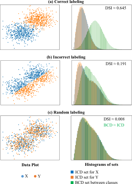
An example of two-class dataset is shown in Figure 1. Figure 1a shows that, if the labels are assigned correctly by clustering, the distributions of ICD sets will be different from the BCD set and the DSI will reach the maximum value for this dataset because the two clusters are well separated. For an incorrect clustering, in Figure 1b, the difference between distributions of ICD and BCD sets becomes smaller so that the DSI value decreases. Figure 1c shows an extreme situation, that is, if all labels are randomly assigned, the distributions of the ICD and BCD sets will be nearly identical. It is the worst case of separation for the two-class dataset and its separability (DSI) is close to zero. Therefore, the separability of clusters can be reflected well by the proposed DSI. The DSI ranges from 0 to 1, , and we suppose that the greater DSI value means the dataset is clustered better.
3 Materials
3.1 Compared CVIs
CVIs are used to evaluate the clustering results. In this paper, several internal CVIs including the proposed DSI have been employed to examine the clustering results from different clustering methods (algorithms). To use different clustering methods on a given dataset may obtain different cluster results and thus, CVIs are used to select the best clusters. We choose eight commonly used (classical and recent) internal CVIs and an external CVI - the Adjusted Rand Index (ARI) to compare with our proposed DSI (Table 3.1). The role of ARI is the ground truth for comparison because ARI involves true labels (clusters) of the dataset.
Compared CVIs. \topruleName Optimal Reference \colruleARI MAX (Santos & Embrechts, 2009) [Santos2009On] \colruleDunn index MAX (Dunn, J.,1973) [Dunn1974Well-Separated] Calinski-Harabasz Index MAX (Calinski & Harabasz, 1974) [Calinski1974dendrite] Davies–Bouldin index min (Davies & Bouldin, 1979) [Davies1979Cluster] Silhouette Coefficient MAX (Rousseeuw, 1987) [Rousseeuw1987Silhouettes:] I MAX (U. Maulik, 2002) [Maulik2002Performance] CVNN min (Yanchi L., 2013) [Liu2013Understanding] WB min (Zhao Q., 2014) [Zhao2014WB-index:] CVDD MAX (Lianyu H., 2019) [Hu2019Internal] DSI MAX Proposed \botrule {tabnote} Optimal column means the CVI for best case has the minimum or maximum value. The ground truth for comparison.
3.2 Synthetic and real datasets
In this paper, the synthetic datasets for clustering are from the Tomas Barton repository 555https://github.com/deric/clustering-benchmark/tree/master/src/main/resources/datasets/artificial, which contains 122 artificial datasets. Each dataset has hundreds to thousands of objects with several to tens of classes in two or three dimensions (features). We have selected 97 datasets for experiment because the 25 unused datasets have too many objects to run the clustering processing in reasonable time. The names of the 97 used synthetic datasets are shown in LABEL:sec:syn_names. Illustrations of these datasets can be found in Tomas Barton’s homepage 666https://github.com/deric/clustering-benchmark.
The 12 real datasets used for clustering are from three sources: the sklearn.datasets package 777https://scikit-learn.org/stable/datasets, UC Irvine Machine Learning Repository [Dheeru2017UCI] and Tomas Barton’s repository (real world datasets) 888https://github.com/deric/clustering-benchmark/tree/master/src/main/resources/datasets/real-world. Unlike the synthetic datasets, the dimensions (feature numbers) of most selected real datasets are greater than three. Hence, CVIs must be used to evaluate their clustering results rather than plotting clusters as for 2D or 3D synthetic datasets. Details about the 12 real datasets appear in Table 3.2.
The description of used real datasets. \topruleName Title Object# Feature# Class# \colruleIris Iris plants dataset 150 4 3 digits Optical recognition of handwritten digits dataset 5620 64 10 wine Wine recognition dataset 178 13 3 cancer Breast cancer Wisconsin (diagnostic) dataset 569 30 2 faces Olivetti faces dataset 400 4096 40 vertebral Vertebral column data 310 6 3 haberman Haberman’s survival data 306 3 2 sonar Sonar, Mines vs. Rocks 208 60 2 tae Teaching Assistant evaluation 151 5 3 thy Thyroid disease data 215 5 3 vehicle Vehicle silhouettes 946 18 4 zoo Zoo data 101 16 7 \botrule
4 Experiments
In general, there are two strategies to evaluate CVIs using a dataset: 1) to compare with ground truth (real clusters with labels); 2) to predict the number of clusters (classes) by finding the optimal number of clusters as identified by CVIs [Cheng2019Novel].
4.1 Using real clusters
By using datasets’ information of real clusters with labels, the steps to evaluate CVIs are:
-
1.
To obtain clustering results by running different clustering methods (algorithms) on a dataset.
-
2.
To compute CVIs of these clustering results and their ARI (ground truth) using real labels.
-
3.
To compare the values of CVI with ARI.
-
4.
To repeat the former three steps for a new dataset.
In this paper, five clustering algorithms from various categories are used, they are: k-means, Ward linkage, spectral clustering, BIRCH [Zhang1996BIRCH:] and EM algorithm (Gaussian Mixture). The CVIs used for evaluation and comparison are shown in Table 3.1 and the used datasets are introduced in Section 3.2. And we provide two evaluation methods to compare the values of CVIs with the ground truth ARI; they are called Hit-the-best and Rank-difference, which are described as follows.
4.1.1 Evaluation metric: Hit-the-best
For a dataset, clustering results obtained by different clustering algorithms would have different CVIs and ARI. If a CVI gives the best score to a clustering result that also has the best ARI score, this CVI is considered to be a correct prediction (hit-the-best). Table 4.1.1 shows CVIs of clustering results by different clustering methods on a dataset. For the wine dataset, k-means receives the best ARI score and Dunn, DB, WB, I, CVNN and DSI give k-means the best score; and thus, the six CVIs are hit-the-best. If we mark hit-the-best CVIs as 1 and others as 0, CVI scores in Table 4.1.1 can be converted to hit-the-best results (Table LABEL:tab:4) for the wine dataset.
CVI scores of clustering results on the wine recognition dataset. \toprule KMeans Ward Linkage Spectral Clustering BIRCH EM \colruleARI + 0.913 0.757 0.880 0.790 0.897 \colruleDunn + 0.232 0.220 0.177 0.229 0.232 CH + 70.885 68.346 70.041 67.647 70.940 DB - 1.388 1.390 1.391 1.419 1.389 Silhouette + 0.284 0.275 0.283 0.278 0.285 WB - 3.700 3.841 3.748 3.880 3.700 I + 5.421 4.933 5.326 4.962 5.421 CVNN - 21.859 22.134 21.932 22.186 21.859 CVDD + 31.114 31.141 29.994 30.492 31.114 DSI + 0.635 0.606 0.629 0.609 0.634 \botrule {tabnote} CVI for best case has the minimum (-) or maximum (+) value. The first row shows results of ARI as ground truth; other rows are CVIs. Bold value: the best case by the measure of this row.