Topological Indoor Mapping through WiFi Signals

Abstract

The ubiquitous presence of WiFi access points and mobile devices capable of measuring WiFi signal strengths allow for real-world applications in indoor localization and mapping. In particular, no additional infrastructure is required. Previous approaches in this field were, however, often hindered by problems such as effortful map-building processes, changing environments and hardware differences. We tackle these problems focussing on topological maps. These represent discrete locations, such as rooms, and their relations, e.g., distances and transition frequencies. In our unsupervised method, we employ WiFi signal strength distributions, dimension reduction and clustering. It can be used in settings where users carry mobile devices and follow their normal routine. We aim for applications in short-lived indoor events such as conferences.

1 Introduction

Navigating unfamiliar indoor venues, such as conference buildings or fair grounds, is a reoccurring task for many individuals. A map that depicts the particular venue layout is a welcome support which, however, has to be prepared beforehand. Moreover, especially at events, such as scientific conferences, this map can be dynamic and require continuous modifications. Hence, techniques to automatically derive maps for indoor venues are useful for a wide range of events.

Assuming that almost every person attending an event has a WiFi enabled smartphone and that WiFi access points (APs) are ubiquitous, in almost all indoor venues, it is natural to develop mapping procedures that take advantage of these facts. WiFi Signals have often been used for indoor localization and mapping in recent years [8, 31]. Since conventional smartphones can measure signal strengths, in theory, no additional infrastructure or mapping devices are required. However, there are two main problems that arise in such a scenarios: first, it is hard to achieve good localization accuracy through WiFi signals. The reason for this are disturbances of WiFi signals, e.g., changes in the environment or humans blocking signals. Additionally, received signal strength indicator (RSSI) measurements are device dependent due to different hardware specifications. Secondly, it requires much effort to map all relevant sites, i.e., physical locations and to represent them via WiFi signal strengths (called fingerprints). Usually such fingerprints need to be collected manually before the so-called online phase. Approaches for automatic site survey exist, yet, they suffer from other difficulties. They often require specific user trajectories and behavior, e.g., to hold a smartphone in a particular way. More sophisticated methods also require modifications of the WiFi infrastructure by modifying AP software.

In our present work we propose a (lightweight) method for topological indoor mapping [26] from RSSI data recorded by smartphones. We figure that accurate topological maps are favored over inaccurate metric maps, in particular within the scope of short-lived indoor events. Hence, our method derives graphs from RSSI data, in which nodes represent (important) locations, e.g., seminar rooms or a refreshments table, and edges represent transitions between these locations (e.g., hallways or stairways). We argue that modeling locations in that manner is similar to the way that humans perceive and refer to their immediate environment [25]. Apart from the conceptual benefits, our hence coarse-grained modeling comes with the practical advantage that accurate localization is easier to achieve. We cope with the hardware dependence of our measurements as well as signal disturbances by employing RSSI distributions of locations (RSSI likelihoods), which are less error prone than single measurements. Our contributions can be summarized as follows: a) We present a lightweight method for building topological indoor maps from WiFi data. b) We experiment on different clustering- and layout techniques, from which we can derive recommendations for similar applications. c) We demonstrate that neither special user behavior nor technical changes of the WiFi infrastructure are required to achieve practically usable results, as demonstrated by two experiments conducted in real-world scenarios.

2 Related Work

An overview on WiFi localization can be gained in the survey articles by He and Chan [8] and Zafari et al. [31]. Notable early approaches with a lasting influence on the field are Horus [30] and Radar [1]. In both methods, samples of WiFi received signal strength indicators (RSSI) for different locations are collected beforehand in a so-called offline phase. The task in the online phase is to perform localization based on a new set of RSSI measurements. Radar achieves this through $k$-nearest-neighbors in a vector space of RSSI signals. Horus represents locations as probability distributions and solves localization using a maximum-likelihood approach. Both methods require manual effort in building WiFi maps in advance by recording labeled RSSI samples (called fingerprints).

To circumvent manual mapping, simultaneous localization and mapping (SLAM) approaches were adopted to WiFi mapping [17, 7, 29]. These methods are based on pedestrian dead reckoning, which requires additional sensor data, e.g., from accelerometer and gyroscope. However, they were only successful in small controlled scenarios and found to be very sensitive to the accuracy and precision of the used smartphone sensors, which may vary in a practical scenario.

WiFi-based topological indoor maps were created by Shin and Cha [26]. Places are represented as nodes, paths as edges in a graph. In the resulting visualizations, nodes were required to be laid out manually. Hence, much of the topology is not captured in the automatic process. Places are points in a coordinate grid. In contrast to this, our aim is that each node represents a meaningful abstract location, such as a room. The problem of creating topological indoor maps in our sense was introduced by Schaefermeier et al. [23]. In that work, research was focussed on the first steps, namely location representations and distance measures. In this work, we build upon this to create complete topological maps.

3 Problem Statement

Task and Requirements

Our overall goal is to automatically infer topological maps of physical venues from signal strength measurements of WiFi access points (APs). In detail, in our setup people shall carry WiFi enabled smartphones while conducting their business within a physical space, e.g., attending talks in a conference building. These smartphones, equipped with a topological navigation application, passively measure the different signal distributions at different places. A therefrom computed topological map should reflect a) which physical locations do exist, and b) how these locations are related to each other. Physical locations can be, e.g., a kitchen in an office or a seminar room in a conference building.

We require any approach to achieve our goal to be: Independent, i.e., our method should work without any additional infrastructure at the physical locations. Automatic, i.e., our method should not require a specific user behaviour (e.g., pointing the smartphone in walking direction). Effortless, i.e., no user interaction or manual place annotation should be needed. Lightweight, i.e., we aim at using as few data as needed and, moreover, we intend to keep the model complexity as low as possible. To discriminate sets of WiFi measurements, one needs, first, a representation of such measurements, called location fingerprint, and secondly, a dissimilarity function or distance between any two representations.

We employ received signal strength indicator (RSSI) measurements that are often represented as vectors, where each component represents the RSSI of a specific AP measured at particular point in time [1]. In this work we grasp them as probability distributions of RSSI values that are conditioned on locations. This approach is less prone to random fluctuations of single measurements. Moreover, it allows naturally for inferring localization of previously unseen measurements by maximum likelihood and determining a confidence that a measurement was made at a particular location. Hence the name RSSI likelihoods.

Formal Problem Definition

The data basis is constituted by timestamped WiFi observations, e.g., recorded by a smartphone. We draw on the relation between signal strength and physical distance to an AP. Each AP is uniquely identified through a basic service set identifier (BSSID).

Definition 1 (WiFi data set)

We call $W\subseteq\mathbb{N}\times D\times B\times R$ WiFi data set, where $\mathbb{N}$ represents timestamps, $D$ is a set of devices, $B$ a set of BSSIDs and $R=[-100,-10]\cap\mathbb{Z}$ a range of RSSI values. A WiFi observation $o\coloneqq(t,d,b,r)\in W$ contains the RSSI value $r$ of WiFi access point $b$ sensed at timestamp $t$ by device $d$. For all $(t,d,b,s_{1}),(t,d,b,s_{2})\in W$ it shall hold that $s_{1}=s_{2}$.

Let the equivalence relation $\check{L}\subseteq W\times W$ reflect the true physical locations, i.e., any two elements of $\check{L}$ represent two distinct physical locations. The classes $[o]_{\check{L}}=\{o^{\prime}\in W\mid(o,o^{\prime})\in\check{L}\}$ give rise to the partition $\check{\mathcal{P}}=W/\check{L}$. The computational problem in our work is to derive an approximation $\mathcal{P}$ of $\check{\mathcal{P}}$, that also allows to lay out useful topological maps. Note, $L\coloneqq\{(u,v)\mid\exists P\in\mathcal{P}:u\in P\land v\in P\}$. For the approximation we investigate different layout methods and clustering techniques. Furthermore, we enrich our data basis for the map building purpose with an acceleration data set, i.e., a relation $A\subset\mathbb{N}\times D\times\mathbb{R}$. An element $(t,d,a)\in A$ represents an acceleration observation, where $a\coloneqq\|\mathbf{a}\|$ for an acceleration vector $\mathbf{a}\in\mathbb{R}^{3}$. This allows us to identify time intervals in which a device is stationary, an information from which we can infer a “preclustering” of $W$.

4 Method

Figure 1: Topological indoor mapping procedure. Each step of our method is depicted as a block. Labels outside blocks refer to their inputs and outputs.

Our method, as depicted in Figure 1, is a sequence of steps that executed in their order lead to the final set of locations. These steps can be seen as conceptual building blocks, which can be realized in different manners. The steps motion mode segmentation, likelihood estimation and distance calculation have been introduced and evaluated in previous work [23]. For completeness, we briefly sum up the recommended methods. For the step layout, we will do an empirical comparison of different methods in Section 5. For the step clustering we select a method based on theoretical and practical considerations.

4.1 Motion Mode Segmentation

The first step of our method exclusively makes use of the acceleration data. In detail, we classify the motion mode of a person into two classes, stationarity or movement. We achieve this by applying a threshold to the energy [5] calculated over short, consecutive time windows. We then summarize all consecutive windows with the same motion mode in a single interval $[t_{i},t_{i+1})$, called motion mode segment. We call $\sigma_{d}=(t_{0},t_{1},\ldots,t_{n})$ the motion mode segmentation of $d$. The idea behind this segmentation process is to combine WiFi observations recorded in segments of stationarity. For one such segment, we exploit the fact that all WiFi observations must have been recorded at a single location. Our reasoning is that single WiFi observations may often be distorted by various signal disturbances, while combining several can mitigate such problems. As a further benefit, we save considerable amounts of battery power by implementing the segmentation directly on the smart device. The reason is that after some time in stationarity we can stop recording further WiFi data, since the signal distribution can already be estimated from the samples recorded up to that point. We set the stopping threshold to five minutes, since this was sufficient for the estimation process.

4.2 Likelihood Estimation

For each stationary motion segment of a device $d$ in an interval $[t_{i},t_{i+1})$, we call the corresponding WiFi observations $W_{d}(t_{i})\subseteq W$ a stationary WiFi segment. For each stationary WiFi segment, we represent the RSSI observations made from each access point $b_{i}\in B$ as a conditional probability distribution $p_{i}(r_{k}\mid L_{d,t_{j}})$. This distribution models the likelihood of receiving RSSI values $r_{k}$ when being at location $L_{d,t_{j}}$. Therefore we call one such distribution RSSI likelihood as an abbreviation. To estimate RSSI likelihoods, we use kernel density estimation (KDE) with a Gaussian kernel and a constant bandwidth derived from background knowledge. We found confirmation that this method improves WiFi localization [20]. Park et al. [20] also found that KDE mitigates the device diversity problem, i.e., localization problems caused by differences in hardware, which in turn lead to different received signal strengths. Different to the aforementioned work, we also model the probability of AP invisibility in our distributions. Each time signal strength is measured by a device $d$ at time $t$ and nothing received from AP $b_{i}$, we add a pseudo-observation $(t,d,b_{i},-100)$ to the WiFi data.

4.3 Distance Calculation

Let $P$ and $Q$ be the cumulative distribution functions of two univariate probability distributions $p$ and $q$ (representing RSSI likelihoods). We calculate their Earth Mover’s Distance (EMD) as $EMD(P,Q)=\int{|P(x)-Q(x)|\mathrm{d}x}$. EMD has several beneficial properties for calculating dissimilarities between RSSI likelihoods. EMD is a true metric and therefore coincides with our view of distances between physical locations in the real world, i.e., in $\mathbb{R}^{2}$ or $\mathbb{R}^{3}$. Furthermore it provides a smooth distance estimate and hence robustness against random differences in the sampled RSSI observations. It has been shown in previous work [23], that between distributions separated by a large gap, EMD approximates the differences between their means. For overlapping distributions, on the other hand, it captures more subtle differences, e.g., between their variances and kurtoses. We combine the distances over all access points using the $L_{1}$ norm. Since EMD returns strictly positive values, the distance between the multivariate RSSI likelihoods $p$ and $q$ becomes the sum $d(p,q)=\sum_{i=1}^{k}{EMD(p_{i},q_{i})}$ over the univariate RSSI likelihoods $p_{i}$ and $q_{i}$ of each AP $b_{i}\in B$. We calculate distances between each pair of RSSI likelihoods and hence obtain a quadratic distance matrix $(d_{ij})$.

4.4 Layout

Through the calculated distances between WiFi segments, we gain information about their relative positions in some abstract signal space. Clustering algorithms, which we use in further steps, in the general case, depend on absolute positions, i.e., coordinates. Therefore we lay out segments in a $p$-dimensional space using three different methods (also called embedding algorithms): Multidimensional Scaling (MDS), t-distributed Stochastic Neighborhood Embedding (t-SNE) and Uniform Manifold Approximation and Projection (UMAP). We chose MDS and t-SNE for being arguably the most widely used methods and UMAP as being a more recent state-of-the-art reported to perform well in, e.g., clustering [21].

Our intuition with embeddings is that the WiFi data is situated in a two- (for a single floor) or three-dimensional (for several floors) subspace of the original signal space. In this subspace, topological relations between physical locations are retained, i.e., measurements that are close in signal space arise from physically close locations. As a side-effect, we conjecture that because input distances can only approximately be retained, some noise and distortions are removed. We may note that the three methods are sometimes regarded as methods for visualization, and there is some dispute on the appropriateness of applying them before clustering. However, they have successfully been used in such scenarios before [28, 21] and there have been some theoretical arguments for this application [12, 10]. Finally, we will use them for visual comparisons of the discovered layouts to the ground truth. Having different properties, the three methods may reveal and emphasize different aspects of the topological relations between locations.

Multidimensional Scaling (MDS)

Multidimensional scaling [16] finds coordinates in $\mathbb{R}^{p}$, such that the input distances $d_{ij}$ between the input pairs are retained as closely as possible. More formally, it finds coordinates $x_{i}\in\mathbb{R}^{p}$ for a chosen $p\in\mathbb{N}$ which minimize the so-called stress, i.e., the function $S(x_{1},x_{2},\cdots,x_{n})=\sum_{i\neq j}{(d_{ij}-{\|x_{i}-x_{j}\|})^{2}}$. In the case where the $d_{ij}$ arise from a metric, such as the EMD, the distance matrix $(d_{ij})$ is symmetric and a triangle matrix is a sufficient representation. The stress can thus be written as $\sum_{i<j}{(d_{ij}-{\|x_{i}-x_{j}\|})^{2}}$ and can be minimized using the SMACOF algorithm [11].

t-Distributed Stochastic Neighborhood Embedding (t-SNE)

t-SNE [14, 13] finds layouts such that the local neighborhoods of points are preserved and accentuated. This makes resulting data points easier to cluster, because the distance to points from other clusters is emphasized. However, depending on the chosen hyper-parameters, t-SNE may also overemphasize random differences in distances and hence lead to too many clusters. t-SNE tries to preserve affinities, which are joint-probabilities based on Gaussian distributions in the input space and based on Cauchy distributions in the output space.

Uniform Manifold Approximation and Projection (UMAP)

This method [15] creates a high- and a low-dimensional fuzzy topological representation of the input data set. The low-dimensional representation is found by minimizing a cross-entropy measure between the input and output fuzzy sets through stochastic gradient descent. An advantage of UMAP is that it produces stable results for different samples from the same data set while providing a low runtime. Finally, the resulting point sets are often densely concentrated facilitating clustering.

4.5 Clustering

We apply clustering algorithms to the coordinates derived from one of the layout methods. By a clustering $\mathcal{C}$ of a set $X:=\{x_{1},x_{2},\ldots,x_{n}\}$ we denote a partition of $X$, i.e., $\mathcal{C}$ is a set $\mathcal{C}\coloneqq\{C_{1},C_{2},\ldots C_{k}\}$ of $k$ non-empty clusters $C_{i}$ s.t. for all $i\neq j$ it holds that $C_{i}\cap C_{j}=\emptyset$ and ${\bigcup}_{i=1}^{k}{C_{i}}=X$. In our case, data points represent stationary WiFi segments of a device. The partition elements (i.e., sets of WiFi segments) represent locations found in our WiFi data set $W$. Thus, we solve two tasks through clustering: location identification and device localization.

Our expectations for a clustering algorithm are: a) Stability, i.e., the same data set should lead to the same clustering when repeatedly executing the algorithm. Small perturbations in the data set should return a similar clustering. b) Agreement, i.e., the found clusters should match our expectations of physical locations in the real world. We compared these properties over various clustering algorithms and experimented on their behavior. Many algorithms, however, suffer from strong variances in the results. This is for two reasons: first, they are sensitive to outliers. Second, they have elements of randomness, which strongly affect the outcome and may lead to different results in repeated runs. As a further problem, they often require the user to set the number of clusters in advance, which, however, for our problem is unknown. In our case, this translates to finding the right number of locations (in agreement with the number of physical locations).

Based on these considerations, we selected the HDBSCAN algorithm [3], an extension of DBSCAN. This algorithm estimates the density of the underlying point distribution based on the distance of each sample in the data set to its $k$-th nearest neighbor. HDBSCAN determines the number of cluster based on the density of the data and provides robustness detecting outliers.

Since device localization is done a-posterior, i.e., after the whole data set has been collected, the clustering is comparable to what is often called the offline phase in localization methods. In this phase, location samples are collected that are later used for reference. Hence, based on the clustered WiFi data, we can easily perform online (i.e., real-time) device localization in topological maps through a classification method such as, e.g., a maximum likelihood approach.

4.6 Graph Representation

Once we have determined a partition $\mathcal{P}$ of our WiFi data set $W$ through clustering, we can order the locations of devices in time to receive their trajectories.

Definition 2 (Trajectory of a Device)

A trajectory $T_{d}$ of a device $d$ in $W$ with partition $\mathcal{P}$ is a sequence $T_{d}=(L_{d,t_{i}})_{i=1}^{n}$ of its visited locations $L_{d,t}\in\mathcal{P}$ such that $\forall i:(t_{i}<t_{i+1})\land\nexists t^{\prime}:(t_{i}<t^{\prime}<t_{i+1})\land(L_{d,t_{i}}\neq L_{d,t^{\prime}})\land(L_{d,t^{\prime}}\neq L_{d,t_{i+1}})$. The length of $T_{d}$ is the number of location transitions $|T_{d}|:=n-1$. A device’s complete trajectory is the one containing all its locations.

We define an (abstract) topological map as a directed graph where each location is a vertex and each trajectory of length $1$ is an edge. We call this an abstract map as opposed to visualized topological maps.

Definition 3 (Abstract Topological Map)

An abstract topological map of a WiFi data set $W$ with a partition $\mathcal{P}$ is a directed, edge-weighted graph $G=(V,E)$ with $V=W/L=\mathcal{P}$ and $E\subseteq W/L\times W/L$ such that $(u,v)\in E$ iff there exists a trajectory of length $1$ from location $u$ to $v$. Its edge weights are determined through an edge-weight function $w:E\rightarrow\mathbb{R}^{+}$.

Hence, edges are directed and may reflect asymmetric relations between locations. Additionally to the edges, relations are represented by an edge-weight function, for which we conceptualize several options. Let $\mathcal{T}$ be the multiset of all trajectories of length 1 from all devices in a WiFi dataset $W$. By abuse of notation, we denote $\mathcal{T}=\{T_{d}\mid|T_{d}|=1,d\in D\}$ where the same $T_{d}$ can occur multiple times in $\mathcal{T}$. We denote the number of occurrences of $T_{d}$ in $\mathcal{T}$ as $m(T_{d})$.

1. Transition Count: $w_{\tau}:(u,v)\mapsto m(u,v)$. The number of transitions between the locations by any device. This can be imagined as a "trodden path" which solidifies the more often people walk from $u$ to $v$.

2. Transition Probability: $w_{p}:(u,v)\mapsto m(u,v)/\sum_{w\in V}{m(u,w)}$. The number of transitions from $u$ to $v$ relative to the number of transitions from $u$ to any other node. This can be regarded as an estimate of the probability of walking to $v$, given that the current location is $u$ assuming a Markov process.

3. Time Difference: $w_{\Delta}:(u,v)\mapsto median(\{t_{i+1}-t_{i}\mid\exists d\in D,j\in\mathbb{N}:t_{i}=\pi_{j}(\sigma_{d})\land L_{d,t_{i}}=u\land L_{d,t_{i+1}}=v\})$ where $\pi_{j}(\sigma_{d})$ is the $j$-th timestamp in the motion mode segmentation $\sigma_{d}$ (cf. Section 4.1). This is the average transition time between locations as a proxy for their distance. The median is used since it is robust against outliers (i.e., extraordinarily fast or slow transitions).

4. Distance in Signal Space: $w_{\sigma}:(u,v)\mapsto d(u,v)$ for some distance measure $d$, such as the average EMD between the WiFi segments related to $u$ and $v$. Similar to the time difference, this estimates distances between real locations.

The resulting representation can be visualized through one of many graph-drawing algorithms. In our method, so far, we assumed that the data has been collected in advance and the resulting map reflects all visited locations. However, in a practical scenario, such as a conference, one may wish to calculate and visualize maps in real-time. Our method can achieve that by repeating all calculations at different points in time with all data collected up to that moment.

5 Experiments

We designed and conducted three experiments at two different venues. To increase the generalization of our results both venues have different properties, e.g., one does have multiple floors while the other does not. In one experiment we controlled the movement while the other is a real-world experiment. Moreover we employed two different methods to acquire the ground truth to evaluate our results. The experiment was conducted using signals from the 2.4GHz band without any modification to the pre-installed APs. We employ different smartphone devices. In particular, we used three HTC One X+, one Samsung Galaxy S8, one Huawei P20, one Honor 8X, three Samsung Galaxy S2 and four Samsung Galaxy S Plus devices. This diversity allowed us to simulate a more realistic scenario.

5.0.1 SFN Dataset

During a two day congress held at the “Schülerforschungszentrum Nordhessen” (SFN) we recorded two controlled walkarounds by the first author. For this, all smartphones were attached to the back of this person, simulating backpack carrying. While walking to and staying at relevant locations the smartphones collected WiFi data and sent it to a central server. The locations were presentation booths or other relevant rooms, altogether twelve distinct places: Computer Lab, Loft, 3D-Printing, Presentation Room, Workshop, Working Space, Electron Microscope, Conservatory, Sound Lab, Moon Station, Laser Lab, Chemical Lab. The whole building, as depicted in Figure 3, had four floors with a varying number of openly accessible rooms. Each walkaround had a duration of about one hour. We used 13 devices. For ground truth, we installed ESP32 modules in all the relevant rooms. These devices were configured as WiFi APs, such that their presence could be detected by the smartphones whenever they were nearby. The ground truth location for a stationary WiFi segment could then be determined through the ESP32 with the highest average signal strength.

5.0.2 Office Dataset

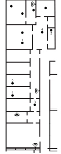
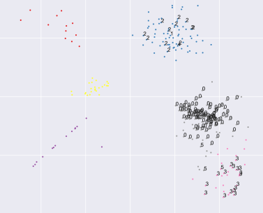
Figure 6: Left: Office floor plan, incl. AP locations and stationary RFIDs (dots). Relevant RFIDs are annotated by numbers. Right: Calculated MDS coordinates per device. Points represent stationary WiFi segments and are clustered through HDBSCAN (one color per cluster). If contacts with stationary RFIDs were registered we annotated points with the ground truth (see floor plan). Unlabeled clusters: canteen, neighboring grocery store, lavatory. Best viewed in color.

We collected WiFi signals and acceleration data from seven individuals at our institute (cf. Figure 6) during one work week (i.e., five full days of work time). This data was collected using eight pairwise different smartphone models. Additionally each participant carried an RFID badge attached to the chest. Together with stationary RFID badges we were able to establish a ground truth location. For technical details about this RFID setup we refer the reader to Schäfermeier et al. [23] and Cattuto et al. [4].

5.1 Measures of Cluster Quality

We assess the quality of clustering WiFi segments using several measures that depend on a ground truth. We decided to employ multiple measures since every measure covers different aspects of accordance to the ground truth. Any clustering depends on the processing step likelihood estimation Section 4.2 and pairwise distance calculation Section 4.3, see Figure 1. For a thorough study on this matter we refer the reader to Schäfermeier et al. [23], from which we use the recommended methods. Furthermore, in our experiments we fix the clustering method to HDBSCAN for the reasons we explained in Section 4.5. The remaining free parameter is the used layout method. Hence, we calculate the evaluation measures for MDS, t-SNE, and UMAP. Since these methods have random components, we perform several runs of the algorithms and report the average scores. We also calculate the standard deviation to provide an idea of the achieved stability.

Table 1: Clustering evaluation for different layout methods. We present the average scores and standard deviations of each cluster quality measure after ten runs of the experiment. The best scores are printed bold and were determined from the average values with a third decimal place not depicted here.

			2D Embedding			3D Embedding
		Method	AMI	ARI	$V$-Meas.	AMI	ARI	$V$-Meas.
Day 1		MDS	.66$\pm$.02	.56$\pm$.02	.75$\pm$.01	.74$\pm$.01	.66$\pm$.01	.82$\pm$.01
		UMAP	.70$\pm$.01	.53$\pm$.02	.80$\pm$.01	.71$\pm$.01	.54$\pm$.02	.81$\pm$.01
		TSNE	.82$\pm$.00	.65$\pm$.01	.84$\pm$.01	.50$\pm$.15	.43$\pm$.15	.55$\pm$.15
Day 2		MDS	.51$\pm$.03	.52$\pm$.03	.57$\pm$.03	.60$\pm$.03	.56$\pm$.07	.67$\pm$.02
		UMAP	.60$\pm$.01	.54$\pm$.04	.72$\pm$.03	.60$\pm$.01	.53$\pm$.03	.71$\pm$.02
		TSNE	.59$\pm$.08	.53$\pm$.11	.71$\pm$.08	.16$\pm$.16	.08$\pm$.11	.21$\pm$.17

For a set $X$, let $\mathcal{C}$ and $\mathcal{K}$ be partitions where the latter is a computed clustering and former is the ground truth. Adjusted Rand index [9]: Let $a\coloneqq|\{\{x,y\}\in{X\choose{2}}\mid\exists C\in\mathcal{C}:\{x,y\}\in C\wedge\exists K\in\mathcal{K}:\{x,y\}\in K\}|$, i.e., $a$ is the number of element pairs such that both elements are assigned to the same cluster within $\mathcal{C}$ as well as $\mathcal{K}$. Dually, let $b\coloneqq|\{\{x,y\}\in{X\choose{2}}\mid\nexists C\in\mathcal{C}:\{x,y\}\in C\wedge\nexists K\in\mathcal{K}:\{x,y\}\in K\}|$. Then $ARI=(RI-\mathbb{E}[RI])/(\max(RI)-\mathbb{E}[RI])$ where $RI=(a+b)/{X\choose{2}}$ is the Rand index. The term $\mathbb{E}[RI]$ is the expected value of $RI$. The Rand index is adjusted such that a random labeling will get an $ARI$ close to zero and the best possible score is 1.0. Adjusted mutual information [18]: Let $P_{\mathcal{C}}(C)$ denote the probability of a random sample $x\in X$ falling into cluster $C$ in the partition $\mathcal{C}$. Respectively, $P_{\mathcal{C}\mathcal{K}}(C,K)$ denotes the probability of a sample belonging to cluster $C$ in $\mathcal{C}$ and to $K$ in $\mathcal{K}$. Based on that the mutual information of $\mathcal{C}$ and $\mathcal{K}$ is defined via $MI(\mathcal{C},\mathcal{K})\coloneqq\sum_{C\in\mathcal{C}}\sum_{K\in\mathcal{K}}P_{\mathcal{C}\mathcal{K}}(C,K)\log(P_{\mathcal{C}\mathcal{K}}(C,K)/(P_{\mathcal{C}}(C)P_{\mathcal{K}}(K)))$. In the following, let $H(\mathcal{C})$ denote the Shannon entropy of partition $\mathcal{C}$. Then the number $AMI=(MI(\mathcal{C},\mathcal{K})-\mathbb{E}[MI(\mathcal{C},\mathcal{K})])/(\max(H(\mathcal{C}),H(\mathcal{K}))-\mathbb{E}[MI(\mathcal{C},\mathcal{K})])$ is the adjusted mutual information, which uses the expected value $\mathbb{E}[MI(\mathcal{C},\mathcal{K})]$ given partitions of the same size as $\mathcal{C}$ and $\mathcal{K}$. Cluster Homogeneity [22]: This measure reflects to what extent elements that are assigned to a cluster belong to the same single class, with respect to the ground truth. The cluster homogeneity is defined by $h(\mathcal{C},\mathcal{K})\coloneqq 1-H(\mathcal{C}|\mathcal{K})/H(\mathcal{C})$, where $H(\mathcal{C}|\mathcal{K})$ denotes the conditional entropy of the class assignment $\mathcal{C}$ given the clustering $\mathcal{K}$. Cluster Completeness [22]: This measure reflects to what extent elements from the same ground truth cluster in $\mathcal{C}$ are assigned to the same cluster in $\mathcal{K}$. Based on that idea is the cluster completeness $c(\mathcal{C},\mathcal{K})\coloneqq 1-(H(\mathcal{K}|\mathcal{C}))/(H(\mathcal{K}))$. $V$-measure [22]: Based on the harmonic mean of cluster homogeneity and cluster completeness the $V$-measure is defined by $V(\mathcal{C},\mathcal{K})=2\cdot h(\mathcal{C},\mathcal{K})\cdot c(\mathcal{C},\mathcal{K})/(h(\mathcal{C},\mathcal{K})+c(\mathcal{C},\mathcal{K}))$. Analogously to $F$-measure for classification, the values of both measures must be high in order to achieve a high value for the $V$-measure.

5.2 Experimental Evaluation of Cluster Quality

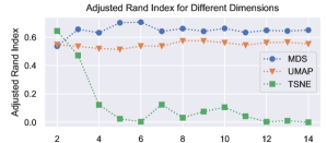
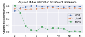
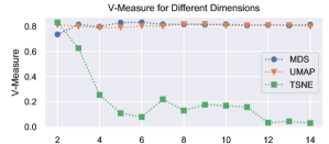
Figure 2: Performance of layout methods for dimensions two to fourteen.

Comparison of 2d embeddings

In our first experiment, we applied all layout algorithms (MDS, t-SNE, UMAP), with a dimension of two, and the subsequent clustering algorithm (HDBSCAN) to the SFN data set. Since our overall goal is to create topological maps, the initial choice for dimension two is natural. We chose SFN, since the ground truth labels for this data set are particularly trustworthy, as they were determined through an additional manual log. To obtain evidence for the stability of the results we conducted each run ten times. We report arithmetic means and standard deviations for the cluster-quality measures in Table 1.

We observe that both UMAP and TSNE give considerably better results than MDS for all of the evaluation measures. Furthermore we note that TSNE performs better than or equal to UMAP in all experiments. Comparing the scores of day 1 with day 2, notably they are higher on the first day. We may note that, even though these values are not comparable due to the different walks performed, the same consequences regarding the compared layout methods apply.

In a visual examination of the plots we found: UMAP leads to plots where points in a cluster are concentrated close together, almost falling into a single point. For TSNE we still get clusters that are clearly distinguishable. However, the points within each cluster are not as densely concentrated. We may note that a more dense plot of a cluster does not necessarily imply a better clustering result with respect to the ground truth, as can be inferred from Table 1.

Comparison of 3d and higher-dimensional embeddings

In the second experiment on the SFN data set, we studied higher-dimensional embeddings. We specifically report our findings on day 1 (see Figure 2), for which we conducted one run per dimension and method. We omit the report on day 2, since results were similar.

First, we find that UMAP and MDS already score close to the best value for a low number of dimensions, i.e., three or four. A further increase in dimension causes only a slight increase of the scores. Hence, it seems that the three dimensional embedding space is sufficient to capture the WiFi signal space that arises from the underlying three-dimensional space. Second, although TSNE achieved the best scores for dimension two (Table 1) they decrease for higher dimensions. In this case, MDS is the method that gives the best results.

These results motivated us to settle for dimension three for the rest of this investigation, which we also report in Table 1, We find that MDS in 3d performs similar well as TSNE in 2d and better than 2d MDS. TSNE, as already seen in Figure 2 performs worse in 3d. MDS performs better than UMAP in most cases, although scores are often similar. Overall, from our experiments, we concluded that multidimensional scaling is the method of choice for the layout step. We also concluded that using the dimension number of the underlying physical space should be used, i.e., for a venue with several floors, we use 3d embeddings.

5.3 Generated Maps

Based on our method we generated topological maps for the SFN and office data set using MDS as depicted in Figures 6, 3 and 3. For both cases, we show floor plans of the building and the embedded and clustered WiFi segments. For the office data set, we use 2d embeddings since the experiment was conducted in a single-floor building. As can be seen, the ground truth locations can be recovered. Moreover, we find that the topological relations between locations are accurately captured. In detail, one can infer the physical floor plan from this plot to some extent. However, we find that in a few cases neighboring locations fall together into a single cluster. This can be attributed to the underlying WiFi signals being similar when being close to the wall between two rooms. We also observed that the layout of the WiFi APs within buildings contributes to the performance.

We created a demo application for the depiction of topological maps during events. The application displays the recognized locations and constructs a topological map of them (Figure 4). Furthermore, it allows to display and track the locations of devices over time and shows the transition probabilities. Locations, which in our model are represented as graph nodes, are depicted as circles. The thickness of a line between the nodes represents the edge weight (cf. Section 4.6). The locations of devices in this map are visualized as dots inside the nodes, in our example there is only one device.

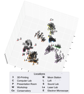
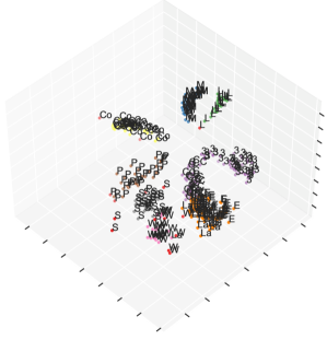
Figure 3: Top: SFN wifi segment layout and clustering for day 2. Each segment is annotated with its ground truth location and colored by its cluster. Outliers are red. Two locations were omitted in the experiment since access was currently not possible. Best viewed in color; Bottom: Floor plan of the venue where the SFN data set was recorded. In this figure, locations of self-installed WiFi access points (ESP32 modules) are given.

5.4 Location Log Comparison of Segments and Ground Truth

Our mapping procedure allows us to extract location logs for devices as depicted in Table 2, in which each row represents a stationary WiFi segment over time. The location column here contains the ground truth locations (determined through the ESP32 controllers). We used these location logs as a compact representation of the results of our method that can, e.g., be compared to manual logs.

As an example, we gathered a manual location log at the office venue with forty-five log entries, from which forty-two entries were inferred correctly through our method. In one case, a single entry in our log was recognized as two segments. In two cases, the determined ground truth annotation was mistaken for an adjacent room, since the walls here were very thin and the ESP32 controller in the same room was slightly rotated. Altogether, although we do not systematically quantify these results, we found our motion mode segmentation as well as our system for determining the ground truth to function reasonably well.

Table 2: Illustrative example for a location log of a device.

Location	Start	End	Duration
Loc. A	Day 1 09:26:04	Day 1 09:26:44	00:00:39
Loc. B	Day 1 09:26:50	Day 1 09:27:01	00:00:11
Loc. C	Day 1 09:27:06	Day 1 09:27:12	00:00:06
Loc. B	Day 1 09:27:17	Day 1 09:27:35	00:00:18
Loc. D	Day 1 09:27:47	Day 1 09:28:01	00:00:14

5.5 Signal Strength Distributions at Locations

We combine all segments from a cluster into an overall RSSI likelihood by averaging over the estimated densities for each WiFi segment (Figure 5). An alternative method would have been a kernel density estimation over the samples from the WiFi segments. We favor the first method to avoid single, very long segments dominating the overall estimation. Our choice leads to slightly different positions being incorporated in the overall estimate. Based on these representations of our final locations, we can achieve localization for new WiFi observations in our abstract topological map. More specifically, for a WiFi observation, i.e., a vector of RSSI values over all APs, we can achieve localization through maximum likelihood [30]. The inferred locations of devices can be, e.g., used for creating a live view of a topological map at some venue, such as a conference or workshop.

5.6 Movement Analysis

In our experiments we found that people in an office scenario are stationary for more than $95\%$ of the time. We figure that for the envisioned applications, such as conferences and workshops, this observation will be replicated to some extent. Hence we base our analyses on stationary segments. We claim that the information conveyed accurately represents the topological locations and relations. This claim is supported by the fact that movement is mostly done between locations of interest while locations visited during movement are mostly hallways.

6 Outlook

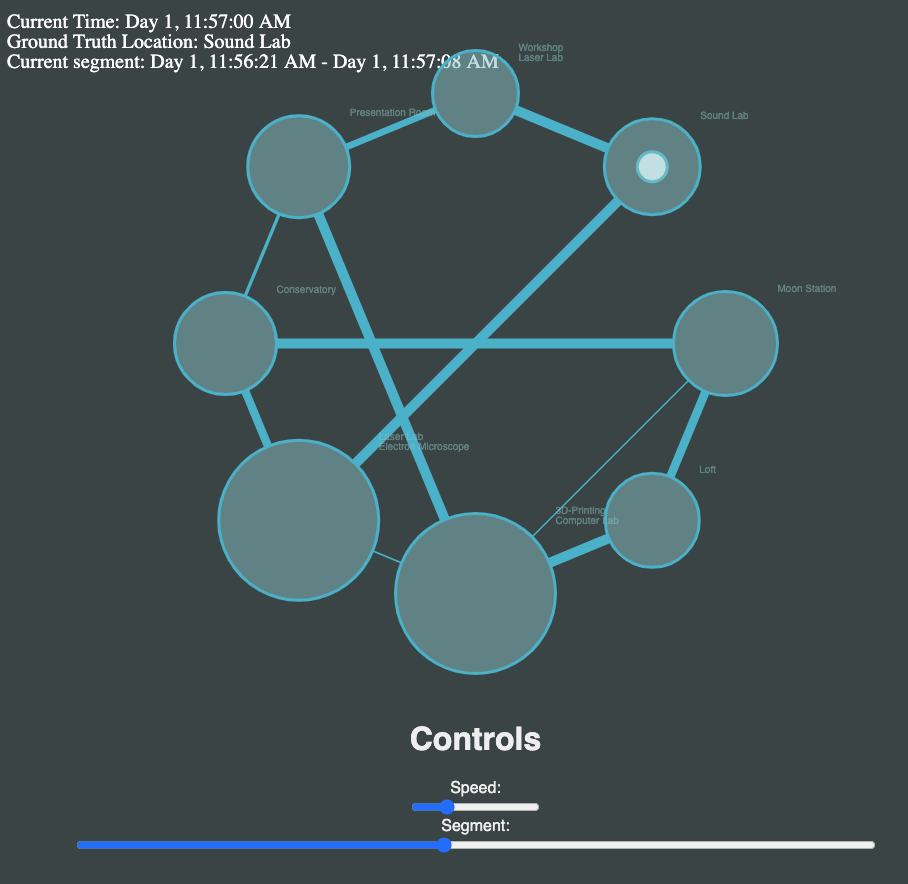
Figure 4: Topological map demo generated for the SFN data set.

We presented a simple and lightweight method to derive meaningful topological maps from WiFi data. In particular, we demonstrated that this is possible without any modifications to the infrastructure of a venue. We showed in experiments conducted at two different venues that we can identify physical locations and recover their topological relations. Our study shows, that overall multidimensional scaling performs best for the layout and clustering task. We found evidence that using the dimension of the venue, i.e., 3d for multistory buildings and 2d for single floors, leads to favorable results. Hence, we conjecture that the intrinsic dimension of the data reflects the physical dimension to some extent. Furthermore, in our experiments, it transpired that the employed methods for motion mode segmentation, likelihood estimation and distance computation are suitable for the localization and mapping problem. Our mapping process relies on the clustering method HDBSCAN, which turned out to be robust, as reflected by low standard deviations of the cluster quality measures. Moreover, apart from few exceptions, it reliably determined the correct number of physical locations. We showed a suitable graph representation for our topological maps. As a notable feature, we presented four different weight functions that reflect different aspects of distances or user transitions between locations. We envision that these weights will be useful for the analysis of social patterns in the realm of events, such as conferences or fairs. Also these edge weights can convey interesting information, when visualized within the final result of our method, i.e., topological maps.

We see many connections of our analysis methods to current research in the area of ubiquitous computing. The next logical step is to enhance our maps with location semantics, e.g., recognizing a registration desk at a conference venue. One can also imagine to automatically derive topical descriptions [24] for locations based on volunteered publication data from the conference participants. As a limitation, we noticed that the device diversity problem could be addressed through more sophisticated methods. The graph drawings could be improved further by adopting, e.g., temporal graph drawing algorithms, which preserve the mental map of users [2, 6, 19]. Finally, a particularly interesting application would be to analyze user trajectories, with methods such as HypTrails [27].

Appendix 0.A Complementary Visualizations

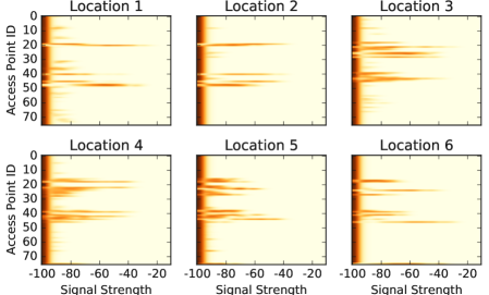
Figure 5: Signal Strength Distributions at Locations. Each subplot depicts the RSSI likelihood given a discovered location. Each row on the y-axis of a subplot represents the signal strength distribution an access point. Colors indicate estimated probabilities. Plots are given for an exemplary subset of the locations discovered by our method in the SFN walkaround 1 data set.

References

- [1] P. Bahl and V. N. Padmanabhan “RADAR: An In-Building RF-Based User Location and Tracking System” In Proc. IEEE INFOCOM 2000 IEEE, 2000, pp. 775–784 URL: http://ieeexplore.ieee.org/xpl/mostRecentIssue.jsp?punumber=6725
- [2] Ulrik Brandes and Steven R. Corman “Visual unrolling of network evolution and the analysis of dynamic discourse?” In Inf. Vis. 2.1, 2003, pp. 40–50 URL: http://dblp.uni-trier.de/db/journals/ivs/ivs2.html#BrandesC03
- [3] R. J. G. B. Campello, D. Moulavi and J. Sander “Density-Based Clustering Based on Hierarchical Density Estimates.” In PAKDD (2) 7819, LNCS Springer, 2013, pp. 160–172
- [4] C. Cattuto et al. “Dynamics of person-to-person interactions from distributed RFID sensor networks” In PloS one 5.7 Public Library of Science, 2010, pp. e11596
- [5] Mostafa Elhoushi, Jacques Georgy, Aboelmagd Noureldin and Michael J. Korenberg “A Survey on Approaches of Motion Mode Recognition Using Sensors” In IEEE Trans. Intell. Transp. Syst. 18.7, 2017, pp. 1662–1686
- [6] Cesim Erten et al. “Exploring the computing literature using temporal graph visualization.” In Visualization and Data Analysis 5295, SPIE Proceedings SPIE, 2004, pp. 45–56 URL: http://dblp.uni-trier.de/db/conf/vda/vda2004.html#ErtenHKWY04
- [7] B. Ferris, D. Fox and N. D. Lawrence “WiFi-SLAM Using Gaussian Process Latent Variable Models.” In IJCAI, 2007, pp. 2480–2485 URL: http://dblp.uni-trier.de/db/conf/ijcai/ijcai2007.html#FerrisFL07
- [8] S. He and S. G. Chan “Wi-Fi Fingerprint-Based Indoor Positioning: Recent Advances and Comparisons” In IEEE Communications Surveys Tutorials 18.1, 2016, pp. 466–490 DOI: 10.1109/COMST.2015.2464084
- [9] Lawrence Hubert and Phipps Arabie “Comparing partitions” In J. of Classification 2.1, 1985, pp. 193–218 URL: http://dx.doi.org/10.1007/BF01908075
- [10] Dmitry Kobak et al. “Heavy-Tailed Kernels Reveal a Finer Cluster Structure in t-SNE Visualisations” In ECML/PKDD (1) 11906, LNCS Springer, 2019, pp. 124–139
- [11] Jan Leeuw “Applications of Convex Analysis to Multidimensional Scaling” In Recent Developments in Statistics Amsterdam: North Holland Publishing Company, 1977, pp. 133–146
- [12] George C. Linderman and Stefan Steinerberger “Clustering with t-SNE, Provably” In SIAM J. Math. Data Sci. 1.2, 2019, pp. 313–332
- [13] Laurens Maaten “Learning a Parametric Embedding by Preserving Local Structure.” In AISTATS 5, JMLR Proceedings JMLR.org, 2009, pp. 384–391 URL: http://dblp.uni-trier.de/db/journals/jmlr/jmlrp5.html#Maaten09
- [14] Laurens Maaten and Geoffrey Hinton “Visualizing Data using t-SNE” In Journal of Machine Learning Research 9, 2008, pp. 2579–2605 URL: http://www.jmlr.org/papers/v9/vandermaaten08a.html
- [15] Leland McInnes, John Healy and James Melville “UMAP: Uniform Manifold Approximation and Projection for Dimension Reduction” cite arxiv:1802.03426, 2018 URL: http://arxiv.org/abs/1802.03426
- [16] A. Mead “Review of the Development of Multidimensional Scaling Methods” In Journal of the Royal Statistical Society. Series D (The Statistician) 41.1 [Royal Statistical Society, Wiley], 1992, pp. 27–39 URL: http://www.jstor.org/stable/2348634
- [17] P. W. Mirowski, T. K. Ho, S. Yi and M. MacDonald “SignalSLAM: Simultaneous localization and mapping with mixed WiFi, Bluetooth, LTE and magnetic signals” In Int. Conf. on Indoor Positioning and Indoor Navigation, IPIN 2013, 2013, pp. 1–10 DOI: 10.1109/IPIN.2013.6817853
- [18] Xuan Vinh Nguyen, Julien Epps and James Bailey “Information Theoretic Measures for Clusterings Comparison: Variants, Properties, Normalization and Correction for Chance.” In J. Mach. Learn. Res. 11, 2010, pp. 2837–2854 URL: http://dblp.uni-trier.de/db/journals/jmlr/jmlr11.html#NguyenEB10
- [19] Stephen C. North “Incremental Layout in DynaDAG.” In Graph Drawing 1027, LNCS Springer, 1995, pp. 409–418 URL: http://dblp.uni-trier.de/db/conf/gd/gd95.html#North95
- [20] Jun Park, Dorothy Curtis, Seth J. Teller and Jonathan Ledlie “Implications of device diversity for organic localization.” In INFOCOM IEEE, 2011, pp. 3182–3190 URL: http://dblp.uni-trier.de/db/conf/infocom/infocom2011.html#ParkCTL11
- [21] Ronald M Parra-Hernández, Jorge I Posada-Quintero, Orlando Acevedo-Charry and Hugo F Posada-Quintero “Uniform Manifold Approximation and Projection for Clustering Taxa through Vocalizations in a Neotropical Passerine (Rough-Legged Tyrannulet, Phyllomyias burmeisteri)” In Animals 10.8 Multidisciplinary Digital Publishing Institute, 2020, pp. 1406
- [22] Andrew Rosenberg and Julia Hirschberg “V-Measure: A Conditional Entropy-Based External Cluster Evaluation Measure” In Proc.EMNLP-CoNLL, 2007, pp. 410–420
- [23] Bastian Schäfermeier, Tom Hanika and Gerd Stumme “Distances for wifi based topological indoor mapping” In MobiQuitous ACM, 2019, pp. 308–317
- [24] Bastian Schäfermeier, Gerd Stumme and Tom Hanika “Topic space trajectories” In Scientometrics Springer, 2021 DOI: 10.1007/s11192-021-03931-0
- [25] Chaoxia Shi, Yanqing Wang and Jingyu Yang “Online topological map building and qualitative localization in large-scale environment” In Robotics and Autonomous Systems 58.5 Elsevier BV, 2010, pp. 488–496 DOI: 10.1016/j.robot.2010.01.009
- [26] H. Shin and H. Cha “Wi-Fi Fingerprint-Based Topological Map Building for Indoor User Tracking” In 16th IEEE RTCSA IEEE Computer Society, 2010, pp. 105–113 DOI: 10.1109/RTCSA.2010.23
- [27] Philipp Singer, Denis Helic, Andreas Hotho and Markus Strohmaier “HypTrails: A Bayesian Approach for Comparing Hypotheses About Human Trails on the Web” In Proceedings of the 24th International Conference on World Wide Web, WWW ’15 Florence, Italy: International World Wide Web Conferences Steering Committee, 2015, pp. 1003–1013 DOI: 10.1145/2736277.2741080
- [28] Erdogan Taskesen and Marcel J. T. Reinders “2D Representation of Transcriptomes by t-SNE Exposes Relatedness between Human Tissues” In PLOS ONE 11.2 Public Library of Science, 2016, pp. 1–6 DOI: 10.1371/journal.pone.0149853
- [29] H. Xiong and D. Tao “A Diversified Generative Latent Variable Model for WiFi-SLAM.” In AAAI AAAI Press, 2017, pp. 3841–3847
- [30] M. Youssef and A. Agrawala “The Horus WLAN location determination system” In MobiSys ’05: Proceedings of the 3rd international conference on Mobile systems, applications, and services Seattle, Washington: ACM, 2005, pp. 205–218 DOI: 10.1145/1067170.1067193
- [31] Faheem Zafari, Athanasios Gkelias and Kin K. Leung “A Survey of Indoor Localization Systems and Technologies” In IEEE Communications Surveys Tutorials 21.3, 2019, pp. 2568–2599 DOI: 10.1109/COMST.2019.2911558